Heiken Ashi Supertrend ADX - StrategyHeiken Ashi Supertrend ADX Strategy
Overview
This strategy combines the power of Heiken Ashi candles, Supertrend indicator, and ADX filter to identify strong trend movements across multiple timeframes. Designed primarily for the cryptocurrency market but adaptable to any tradable asset, this system focuses on capturing momentum in established trends while employing a sophisticated triple-layer stop loss mechanism to protect capital and secure profits.
Strategy Mechanics
Entry Signals
The strategy uses a unique blend of technical signals to identify high-probability trade entries:
Heiken Ashi Candles: Looks specifically for Heiken Ashi candles with minimal or no wicks, which signal strong momentum and trend continuation. These "full-bodied" candles represent periods where price moved decisively in one direction with minimal retracement.
Supertrend Filter : Confirms the underlying trend direction using the Supertrend indicator (default factor: 3.0, ATR period: 10). Entries are aligned with the prevailing Supertrend direction.
ADX Filter (Optional) : Can be enabled to focus only on stronger trending conditions, filtering out choppy or ranging markets. When enabled, trades only trigger when ADX is above the specified threshold (default: 25).
Exit Signals
Positions are closed when either:
An opposing signal appears (Heiken Ashi candle with no wick in the opposite direction)
Any of the three stop loss mechanisms are triggered
Triple-Layer Stop Loss System
The strategy employs a sophisticated three-tier stop loss approach:
ATR Trailing Stop: Adapts to market volatility and locks in profits as the trend extends. This stop moves in the direction of the trade, capturing profit without exiting too early during normal price fluctuations.
Swing Point Stop : Uses natural market structure (recent highs/lows over a lookback period) to place stops at logical support/resistance levels, honoring the market's own rhythm.
Insurance Stop: A percentage-based safety net that protects against sudden adverse moves immediately after entry. This is particularly valuable when the swing point stop might be positioned too far from entry, providing immediate capital protection.
Optimization Features
Customizable Filters: All components (Supertrend, ADX) can be enabled/disabled to adapt to different market conditions
Adjustable Parameters: Fine-tune ATR periods, Supertrend factors, and ADX thresholds
Flexible Stop Loss Settings: Each of the three stop loss mechanisms can be individually enabled/disabled with customizable parameters
Best Practices for Implementation
Recommended Timeframes: Works best on 4-hour charts and above, where trends develop more reliably
Market Conditions: Performs well across various market conditions due to the ADX filter's ability to identify meaningful trends
Position Sizing: The strategy uses a percentage of equity approach (default: 3%) for position sizing
Performance Characteristics
When properly optimized, this strategy has demonstrated profit factors exceeding 3 in backtesting. The approach typically produces generous winners while limiting losses through its multi-layered stop loss system. The ATR trailing stop is particularly effective at capturing extended trends, while the insurance stop provides immediate protection against adverse moves.
The visual components on the chart make it easy to follow the strategy's logic, with position status, entry prices, and current stop levels clearly displayed.
This strategy represents a complete trading system with clearly defined entry and exit rules, adaptive stop loss mechanisms, and built-in risk management through position sizing.
Cerca negli script per "profit"

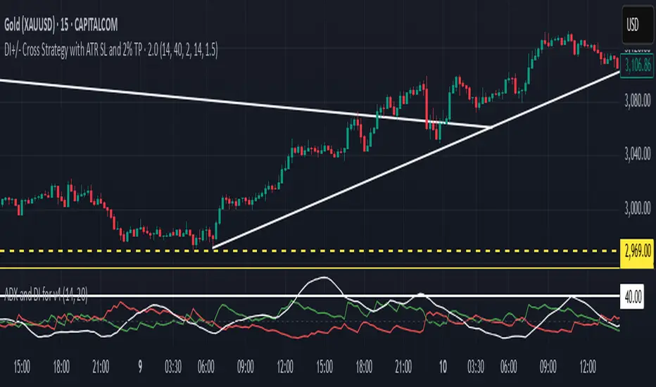
DI+/- Cross Strategy with ATR SL and 2% TPDI+/- Cross Strategy with ATR Stop Loss and 2% Take Profit
📝 Script Description for Publishing:
This strategy is based on the directional movement of the market using the Average Directional Index (ADX) components — DI+ and DI- — to generate entry signals, with clearly defined risk and reward targets using ATR-based Stop Loss and Fixed Percentage Take Profit.
🔍 How it works:
Buy Signal: When DI+ crosses above 40, signaling strong bullish momentum.
Sell Signal: When DI- crosses above 40, indicating strong bearish momentum.
Stop Loss: Dynamically calculated using ATR × 1.5, to account for market volatility.
Take Profit: Fixed at 2% above/below the entry price, for consistent reward targeting.
🧠 Why it’s useful:
Combines momentum breakout logic with volatility-based risk management.
Works well on trending assets, especially when combined with higher timeframe filters.
Clean BUY and SELL visual labels make it easy to interpret and backtest.
✅ Tips for Use:
Use on assets with clear trends (e.g., major forex pairs, trending stocks, crypto).
Best on 30m – 4H timeframes, but can be customized.
Consider combining with other filters (e.g., EMA trend direction or Bollinger Bands) for even better accuracy.
RSI VWAP POC [Uncle Sam Trading]Category: Oscillators, Volume, Market Profile
Timeframe: Suitable for all timeframes
Markets: Crypto, Forex, Stocks, Commodities
Overview
The RSI VWAP POC indicator is a powerful and innovative oscillator that combines the Relative Strength Index (RSI), Volume-Weighted Average Price (VWAP), and Point of Control (POC) from market profile analysis. Designed to provide traders with clear, high-probability trading signals, this indicator helps you identify key market levels, spot overbought/oversold conditions, and time your entries and exits with precision. Whether you’re a day trader, swing trader, or scalper, this free tool adds significant value to your trading strategy by offering a unique blend of momentum, volume, and market profile insights.
How It Works
This indicator integrates three core components to deliver actionable insights:
RSI (Relative Strength Index): Measures momentum to identify overbought (above 70) and oversold (below 30) conditions, helping you anticipate potential reversals.
VWAP (Volume-Weighted Average Price): Calculates a volume-weighted price benchmark, which is used to compute a more accurate, volume-sensitive RSI. This ensures the indicator reflects true market dynamics.
POC (Point of Control): Derived from market profile analysis, the POC represents the price level with the highest traded volume in a session, acting as a critical support or resistance level.
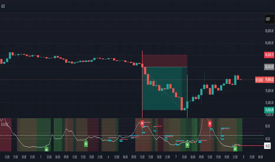
The indicator plots a smoothed RSI based on VWAP, overlaid with market profile data on a user-defined higher timeframe (default: 4H). The POC is displayed as a red line, with aqua bars indicating the value area where the majority of trading volume occurred. When the RSI crosses the POC, the indicator generates clear buy and sell signals:
Strong Buy (SBU): RSI crosses above the POC in an oversold zone.
Strong Sell (SBD): RSI crosses below the POC in an overbought zone.
Additional features include:
Background colors to highlight bullish (green) or bearish (red) trends.
Shaded zones for overbought (70/60) and oversold (30/40) levels.
Customizable settings to fit your trading style and timeframe.
How This Indicator Adds Value
The RSI VWAP POC indicator offers several key benefits that enhance your trading performance:
High-Probability Signals: By combining RSI, VWAP, and POC, this indicator identifies trades at key market levels where price is likely to react, increasing your win rate.
Improved Timing: Clear buy and sell signals, such as ‘SBU’ and ‘SBD’, help you enter and exit trades at optimal points, maximizing profitability.
Risk Management: Overbought/oversold zones and trend confirmation via background colors help you avoid false signals, protecting your capital.
Versatility: Suitable for all markets (crypto, forex, stocks) and timeframes, making it a valuable tool for traders of all experience levels.
Time Efficiency: The indicator does the heavy lifting by analyzing momentum, volume, and market profile data, allowing you to focus on executing trades.
Real-World Performance Example: On a 1-hour Bitcoin chart with a 4-hour higher timeframe, this indicator identified a strong sell signal on April 6th at 12:00 ($82,000), leading to a 9% drop to $74,600. A subsequent strong buy signal on April 7th at 04:00 ($76,200) captured a 6% rise to $81,200 – a potential 25% profit with 5x leverage if exited at 5%.
How to Use
Add the Indicator: Search for “RSI VWAP POC ” in TradingView’s indicator library and add it to your chart.
Set Your Timeframe: The indicator works on any timeframe but is optimized for a 1-hour chart with a 4-hour higher timeframe (set in the settings).
Interpret Signals:
Look for ‘SBU’ (strong buy) labels when the RSI crosses above the POC in an oversold zone, indicating a potential buying opportunity.
Look for ‘SBD’ (strong sell) labels when the RSI crosses below the POC in an overbought zone, signaling a potential selling opportunity.
Use the background colors (green for bullish, red for bearish) to confirm the trend.
Combine with Your Strategy: Use the indicator alongside your existing analysis (e.g., support/resistance, candlestick patterns) for best results.
Settings and Customization
The indicator is highly customizable to suit your trading needs:
RSI Length (Default: 14): Adjust the sensitivity of the RSI. Use a shorter length (e.g., 10) for scalping, or a longer length (e.g., 20) for smoother signals.
EMA Smoothing Length (Default: 3): Smooths the RSI line. Increase to 5 or 7 for less choppy signals in volatile markets.
Higher Timeframe (Default: 240 minutes): Set to 240 (4 hours) for a 1-hour chart. Adjust based on your chart’s timeframe (e.g., 60 minutes for a 15-minute chart).
Value Area Percentage (Default: 100%): Defines the size of the value area around the POC. Lower to 70% for a tighter focus on key levels.
Overbought/Oversold Thresholds (Defaults: 70/30): Adjust these levels to match market conditions (e.g., 80/20 for trending markets).
Show POC Line (Default: True): Toggle the red POC line on or off.
Show Buy/Sell Signals: Enable ‘Show Strong Breakup Signals’ and ‘Show Strong Breakdown Signals’ to focus on high-probability trades.
Why Choose This Indicator?
The RSI VWAP POC indicator stands out by offering a unique combination of momentum, volume, and market profile analysis in a single, easy-to-use tool. It’s designed to help traders of all levels make informed decisions, reduce risk, and increase profitability. Whether you’re trading Bitcoin, forex pairs, or stocks, this indicator provides the clarity and precision you need to succeed.
Portfolio Monitor - DolphinTradeBot1️⃣ Overview
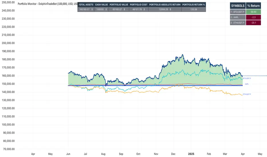
▪️This indicator unifies the value of all your investments—whether stocks, currencies, or cryptocurrencies—in your chosen currency. This tool not only provides a clear snapshot of your overall portfolio performance but also highlights the individual growth of each asset with intuitive visualizations and an easy-to-understand performance report.
2️⃣ What sets this indicator apart
▪️is its ability to convert values from various currency pairs into any currency you choose. This means you can monitor your portfolio's performance against any currency pair you prefer, offering a flexible and comprehensive view of your investments.
3️⃣ How Is It Work ?
🔍The indicator can be analyzed under two main categories: visual representations and tables.
1- Visual representations ;
The indicator includes three different types of lines:
1. 1 - Reference Line → This represents the cost of all assets we hold, based on the selected date.
1. 2 - Total Assets Line → Displays the real-time value of all assets in our possession, including cash value, in the selected trading pair.
The area between the reference line is filled with green and red. The section above the reference line is represented in green, while the section below is shown in red.
1. 3 - Performance Lines → These visualize the performance of the assets, starting from the reference line and taking into account their weights in the portfolio. (Note: The lines are scaled for visualization purposes, so their absolute values should not be considered.)
"The names of the lines are shown in the image below."⤵️
2- Tables
The indicator includes three different types of tables:
2. 1 - Analysis Table : It provides a superficial overview of wallet statistics and values.
▪️TOTAL ASSETS → The current equivalent of all assets in the target currency
▪️CASH VALUE → The current value of the amount "Cash Value", in the target currency.
▪️PORTFOLIO VALUE → The total value of assets excluding Cash, in the target currency.
▪️POSTFOLIO COST → The cost of assets excluding Cash, in the target currency.
▪️PORTFOLIO ABSOLUTE RETURN → It shows the profit or loss relative to the cost of assets
▪️PORTFOLIO RETURN % →It shows the profit or loss relative to the cost of assets on a percentage basis
2. 2 - Performance Table : It displays the names of assets excluding Cash and their profit amounts, sorted from highest to lowest profit. If "Show as Percentage" is selected in the settings, it shows the percentage profit or loss relative to the cost. Profits are represented in green, while losses are represented in red.
"You can see the visual showing the tables below"⤵️
4️⃣How to Use ?
1- Choose the date on which the visualization will begin (📌The start date only affects the exchange rate used for calculating the reference line in the target currency.)
2- If you have cash holdings, enter the amount and specify the currency.
3- Select the currency in which your portfolio value will be displayed.(Default value is USD)
4- To set up your portfolio;
SYMBOLS - QUANTITY - PURCHASE PRICE
Enter the symbols of your assets - the number of units you hold - and their cost levels.
5- If you have cash, be sure to include your cash balance. If you also hold other currencies, enter them as separate assets with their corresponding quantities and purchase prices.
6- If you want to see the percentage returns of the assets in the performance table relative to their cost, select the "Show as Percent" option.
7- If you want to see the performance visuals of the assets, click on the "Show Asset Performance" option.
You can find an image of the settings section where the numbers above are used as references below.⤵️
📌 NOTE → By default, a few assets and their values have been pre-added in the initial settings. This is to ensure that you don’t see an empty screen when adding the indicator to the chart. Please remember to enter your own assets and values. The default settings are only provided as an example.
Strategy Stats [presentTrading]Hello! it's another weekend. This tool is a strategy performance analysis tool. Looking at the TradingView community, it seems few creators focus on this aspect. I've intentionally created a shared version. Welcome to share your idea or question on this.
█ Introduction and How it is Different
Strategy Stats is a comprehensive performance analytics framework designed specifically for trading strategies. Unlike standard strategy backtesting tools that simply show cumulative profits, this analytics suite provides real-time, multi-timeframe statistical analysis of your trading performance.
Multi-timeframe analysis: Automatically tracks performance metrics across the most recent time periods (last 7 days, 30 days, 90 days, 1 year, and 4 years)
Advanced statistical measures: Goes beyond basic metrics to include Information Coefficient (IC) and Sortino Ratio
Real-time feedback: Updates performance statistics with each new trade
Visual analytics: Color-coded performance table provides instant visual feedback on strategy health
Integrated risk management: Implements sophisticated take profit mechanisms with 3-step ATR and percentage-based exits
BTCUSD Performance
The table in the upper right corner is a comprehensive performance dashboard showing trading strategy statistics.
Note: While this presentation uses Vegas SuperTrend as the underlying strategy, this is merely an example. The Stats framework can be applied to any trading strategy. The Vegas SuperTrend implementation is included solely to demonstrate how the analytics module integrates with a trading strategy.
⚠️ Timeframe Limitations
Important: TradingView's backtesting engine has a maximum storage limit of 10,000 bars. When using this strategy stats framework on smaller timeframes such as 1-hour or 2-hour charts, you may encounter errors if your backtesting period is too long.
Recommended Timeframe Usage:
Ideal for: 4H, 6H, 8H, Daily charts and above
May cause errors on: 1H, 2H charts spanning multiple years
Not recommended for: Timeframes below 1H with long history
█ Strategy, How it Works: Detailed Explanation
The Strategy Stats framework consists of three primary components: statistical data collection, performance analysis, and visualization.
🔶 Statistical Data Collection
The system maintains several critical data arrays:
equityHistory: Tracks equity curve over time
tradeHistory: Records profit/loss of each trade
predictionSignals: Stores trade direction signals (1 for long, -1 for short)
actualReturns: Records corresponding actual returns from each trade
For each closed trade, the system captures:
float tradePnL = strategy.closedtrades.profit(tradeIndex)
float tradeReturn = strategy.closedtrades.profit_percent(tradeIndex)
int tradeType = entryPrice < exitPrice ? 1 : -1 // Direction
🔶 Performance Metrics Calculation
The framework calculates several key performance metrics:
Information Coefficient (IC):
The correlation between prediction signals and actual returns, measuring forecast skill.
IC = Correlation(predictionSignals, actualReturns)
Where Correlation is the Pearson correlation coefficient:
Correlation(X,Y) = (nΣXY - ΣXY) / √
Sortino Ratio:
Measures risk-adjusted return focusing only on downside risk:
Sortino = (Avg_Return - Risk_Free_Rate) / Downside_Deviation
Where Downside Deviation is:
Downside_Deviation = √
R_i represents individual returns, T is the target return (typically the risk-free rate), and n is the number of observations.
Maximum Drawdown:
Tracks the largest percentage drop from peak to trough:
DD = (Peak_Equity - Trough_Equity) / Peak_Equity * 100
🔶 Time Period Calculation
The system automatically determines the appropriate number of bars to analyze for each timeframe based on the current chart timeframe:
bars_7d = math.max(1, math.round(7 * barsPerDay))
bars_30d = math.max(1, math.round(30 * barsPerDay))
bars_90d = math.max(1, math.round(90 * barsPerDay))
bars_365d = math.max(1, math.round(365 * barsPerDay))
bars_4y = math.max(1, math.round(365 * 4 * barsPerDay))
Where barsPerDay is calculated based on the chart timeframe:
barsPerDay = timeframe.isintraday ?
24 * 60 / math.max(1, (timeframe.in_seconds() / 60)) :
timeframe.isdaily ? 1 :
timeframe.isweekly ? 1/7 :
timeframe.ismonthly ? 1/30 : 0.01
🔶 Visual Representation
The system presents performance data in a color-coded table with intuitive visual indicators:
Green: Excellent performance
Lime: Good performance
Gray: Neutral performance
Orange: Mediocre performance
Red: Poor performance
█ Trade Direction
The Strategy Stats framework supports three trading directions:
Long Only: Only takes long positions when entry conditions are met
Short Only: Only takes short positions when entry conditions are met
Both: Takes both long and short positions depending on market conditions
█ Usage
To effectively use the Strategy Stats framework:
Apply to existing strategies: Add the performance tracking code to any strategy to gain advanced analytics
Monitor multiple timeframes: Use the multi-timeframe analysis to identify performance trends
Evaluate strategy health: Review IC and Sortino ratios to assess predictive power and risk-adjusted returns
Optimize parameters: Use performance data to refine strategy parameters
Compare strategies: Apply the framework to multiple strategies to identify the most effective approach
For best results, allow the strategy to generate sufficient trade history for meaningful statistical analysis (at least 20-30 trades).
█ Default Settings
The default settings have been carefully calibrated for cryptocurrency markets:
Performance Tracking:
Time periods: 7D, 30D, 90D, 1Y, 4Y
Statistical measures: Return, Win%, MaxDD, IC, Sortino Ratio
IC color thresholds: >0.3 (green), >0.1 (lime), <-0.1 (orange), <-0.3 (red)
Sortino color thresholds: >1.0 (green), >0.5 (lime), <0 (red)
Multi-Step Take Profit:
ATR multipliers: 2.618, 5.0, 10.0
Percentage levels: 3%, 8%, 17%
Short multiplier: 1.5x (makes short take profits more aggressive)
Stop loss: 20%

AI Trend Momentum SniperThe AI Trend Momentum Sniper is a powerful technical analysis tool designed for day trading. This strategy combines multiple momentum and trend indicators to identify high-probability entry and exit points. The indicator utilizes a combination of Supertrend, MACD, RSI, ATR (Average True Range), and On-Balance Volume (OBV) to generate real-time signals for buy and sell opportunities.
Key Features:
Supertrend for detecting market direction (bullish or bearish).
MACD for momentum confirmation, highlighting changes in market momentum.
RSI to filter out overbought/oversold conditions and ensure high-quality trades.
ATR as a volatility filter to adjust for changing market conditions.
OBV (On-Balance Volume) to confirm volume strength and trend validity.
Dynamic Stop-Loss & Take-Profit based on ATR to manage risk and lock profits.
This indicator is tailored for intraday traders looking for quick market moves, especially in volatile and high liquidity assets like Bitcoin (BTC) and Ethereum (ETH). It helps traders capture short-term trends with efficient risk management tools.
How to Apply:
Set Your Chart: Apply the AI Trend Momentum Sniper to a 5-minute (M5) or 15-minute (M15) chart for optimal performance.
Buy Signal: When the indicator generates a green arrow below the bar, it indicates a buy signal based on positive trend and momentum alignment.
Sell Signal: A red arrow above the bar signals a sell condition when the trend and momentum shift bearish.
Stop-Loss and Take-Profit: The indicator automatically calculates dynamic stop-loss and take-profit levels based on the ATR value for each trade, ensuring proper risk management.
Alerts: Set up custom alerts for buy or sell signals, and get notified instantly when opportunities arise.
Best Markets for Use:
BTC/USDT, ETH/USDT – High liquidity and volatility.
Major altcoins with sufficient volume.
Avoid using it on low-liquidity assets where price action may become erratic.
Timeframes:
This indicator is best suited for lower timeframes (5-minute to 15-minute charts) to capture quick price movements in trending markets.

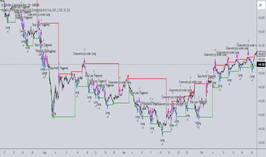
Liquidity + Internal Market Shift StrategyLiquidity + Internal Market Shift Strategy
This strategy combines liquidity zone analysis with the internal market structure, aiming to identify high-probability entry points. It uses key liquidity levels (local highs and lows) to track the price's interaction with significant market levels and then employs internal market shifts to trigger trades.
Key Features:
Internal Shift Logic: Instead of relying on traditional candlestick patterns like engulfing candles, this strategy utilizes internal market shifts. A bullish shift occurs when the price breaks previous bearish levels, and a bearish shift happens when the price breaks previous bullish levels, indicating a change in market direction.
Liquidity Zones: The strategy dynamically identifies key liquidity zones (local highs and lows) to detect potential reversal points and prevent trades in weak market conditions.
Mode Options: You can choose to run the strategy in "Both," "Bullish Only," or "Bearish Only" modes, allowing for flexibility based on market conditions.
Stop-Loss and Take-Profit: Customizable stop-loss and take-profit levels are integrated to manage risk and lock in profits.
Time Range Control: You can specify the time range for trading, ensuring the strategy only operates during the desired period.
This strategy is ideal for traders who want to combine liquidity analysis with internal structure shifts for precise market entries and exits.
This description clearly outlines the strategy's logic, the flexibility it provides, and how it works. You can adjust it further to match your personal trading style or preferences!
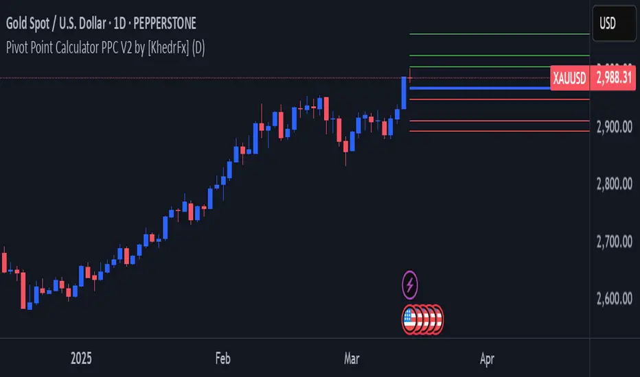
Pivot Point Calculator PPC V2 by [KhedrFx]📈 Trade Smarter with the Pivot Point Calculator (PPC) by KhedrFx
Want to spot key price levels and make better trading decisions? The Pivot Point Calculator (PPC) by KhedrFx is your go-to TradingView tool for identifying potential support and resistance zones. Whether you’re a Scalper trader, day trader, swing trader, or long-term investor, this script helps you plan precise entries and exits with confidence.
🔹 How to Use Pivot Points in Trading
📊 Step 1: Identify Key Levels
The PPC automatically plots:
Pivot Point (P): The main level where sentiment shifts between bullish and bearish.
Support Levels (S1, S2, S3): Areas where price may bounce higher.
Resistance Levels (R1, R2, R3): Areas where price may face selling pressure.
These levels act as dynamic price zones, helping you anticipate potential market movements.
🔥 Step 2: Choose Your Trading Strategy
1️⃣ Breakout Trading
Buy when the price breaks above the pivot point (P) with strong momentum.
Sell when the price drops below the pivot point (P) with strong momentum.
Use R1, R2, or R3 as profit targets in an uptrend and S1, S2, or S3 in a downtrend.
2️⃣ Reversal (Bounce) Trading
Buy when the price pulls back to S1, S2, or S3 and shows bullish confirmation (e.g., candlestick patterns like a bullish engulfing or hammer).
Sell when the price rallies to R1, R2, or R3 and shows bearish confirmation (e.g., rejection wicks or a bearish engulfing pattern).
🎯 Step 3: Set Smart Stop-Loss & Take-Profit Levels
Stop-Loss: Place it slightly below support (for buy trades) or above resistance (for sell trades).
Take-Profit: Use the next pivot level as a target.
Extreme Zones: R3 and S3 often signal strong reversals or breakouts—watch them closely!
🚀 How to Get Started
1️⃣ Add the PPC script to your TradingView chart.
2️⃣ Choose a timeframe that fits your strategy (5m, 15m, 30m, 1H, 4H, Daily, or Weekly).
3️⃣ Use the pivot points and support/resistance levels to fine-tune your trade entries, exits, and risk management.
⚠️ Trade Responsibly
This tool helps you analyze the market, but it’s not a guarantee of profits. Always do your own research, manage risk, and trade with caution.
💡 Ready to take your trading to the next level? Try the Pivot Point Calculator (PPC) by KhedrFx and start trading with confidence today! 🚀
IU BBB(Big Body Bar) StrategyDESCRIPTION
The IU BBB (Big Body Bar) Strategy is a price action-based trading strategy that identifies high-momentum candles with significantly larger body sizes compared to the average. It enters trades when a strong bullish or bearish move occurs and manages risk using an ATR-based trailing stop-loss system.
USER INPUTS:
- Big Body Threshold – Defines how many times larger the candle body should be compared to the average body ( default is 4 ).
- ATR Length – The period for the Average True Range (ATR) used in the trailing stop-loss calculation ( default is 14 ).
- ATR Factor – Multiplier for ATR to determine the trailing stop distance ( default is 2 ).
LONG CONDITION:
- The current candle’s body is greater than the average body size multiplied by the Big Body Threshold.
- The closing price is higher than the opening price (bullish candle).
SHORT CONDITION:
- The current candle’s body is greater than the average body size multiplied by the Big Body Threshold.
- The closing price is lower than the opening price (bearish candle).
LONG EXIT:
- ATR-based trailing stop-loss dynamically adjusts, locking in profits as the price moves higher.
SHORT EXIT:
- ATR-based trailing stop-loss dynamically adjusts, securing profits as the price moves lower.
WHY IT IS UNIQUE:
- Unlike traditional momentum strategies, this system adapts to volatility by filtering trades based on relative candle size.
- It incorporates an ATR-based trailing stop-loss, ensuring risk management and profit protection.
- The strategy avoids choppy market conditions by only trading when significant momentum is present.
HOW USERS CAN BENEFIT FROM IT:
- Catch Strong Price Moves – The strategy helps traders enter trades when the market shows decisive momentum.
- Effective Risk Management – The ATR-based trailing stop ensures that winning trades remain profitable.
- Works Across Markets – Can be applied to stocks, forex, crypto, and indices with proper optimization.
- Fully Customizable – Users can adjust sensitivity settings to match their trading style and time frame.

Simple APF Strategy Backtesting [The Quant Science]Simple backtesting strategy for the quantitative indicator Autocorrelation Price Forecasting. This is a Buy & Sell strategy that operates exclusively with long orders. It opens long positions and generates profit based on the future price forecast provided by the indicator. It's particularly suitable for trend-following trading strategies or directional markets with an established trend.
Main functions
1. Cycle Detection: Utilize autocorrelation to identify repetitive market behaviors and cycles.
2. Forecasting for Backtesting: Simulate trades and assess the profitability of various strategies based on future price predictions.
Logic
The strategy works as follow:
Entry Condition: Go long if the hypothetical gain exceeds the threshold gain (configurable by user interface).
Position Management: Sets a take-profit level based on the future price.
Position Sizing: Automatically calculates the order size as a percentage of the equity.
No Stop-Loss: this strategy doesn't includes any stop loss.
Example Use Case
A trader analyzes a dayli period using 7 historical bars for autocorrelation.
Sets a threshold gain of 20 points using a 5% of the equity for each trade.
Evaluates the effectiveness of a long-only strategy in this period to assess its profitability and risk-adjusted performance.
User Interface
Length: Set the length of the data used in the autocorrelation price forecasting model.
Thresold Gain: Minimum value to be considered for opening trades based on future price forecast.
Order Size: percentage size of the equity used for each single trade.
Strategy Limit
This strategy does not use a stop loss. If the price continues to drop and the future price forecast is incorrect, the trader may incur a loss or have their capital locked in the losing trade.
Disclaimer!
This is a simple template. Use the code as a starting point rather than a finished solution. The script does not include important parameters, so use it solely for educational purposes or as a boilerplate.

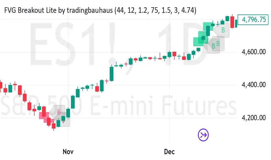
FVG Breakout Lite by tradingbauhausExplanation of "FVG Breakout Lite by tradingbauhaus"
This script is a trading strategy built for TradingView that helps you spot and trade "Fair Value Gaps" (FVGs)—price areas where the market moved quickly, leaving a gap that might act as support or resistance later. It’s designed to catch breakout opportunities when the price moves strongly in one direction, with extra filters to make trades more reliable. Here’s how it works and how you can use it:
What It Does
1. Finds Fair Value Gaps (FVGs):
A "Bullish FVG" happens when the price jumps up quickly, leaving a gap below where it didn’t trade much (e.g., today’s low is higher than the high from two bars ago).
A "Bearish FVG" is the opposite: the price drops fast, leaving a gap above (e.g., today’s high is lower than the low from two bars ago).
The script draws colored boxes on your chart to show these gaps: green for bullish, red for bearish.
2. Spots Breakouts:
It looks for "strong" FVGs by comparing them to a trend (based on the highest highs and lowest lows over a set period).
If a bullish gap forms above the recent highs, or a bearish gap below the recent lows, it’s marked as a breakout opportunity.
3. Adds a Volume Check:
Trades only happen if the market’s volume is higher than usual (e.g., 1.2x the average volume over the last 20 bars). This helps ensure the breakout has real momentum behind it.
4. Trades Automatically:
Long Trades (Buy): If a bullish breakout FVG forms and volume is high, it buys at the current price.
Short Trades (Sell): If a bearish breakout FVG forms with high volume, it sells short.
Each trade comes with a stop loss (to limit losses) and a take profit (to lock in gains), both adjustable by you.
5. Shows Mitigation Lines (Optional):
If you turn on "Display Mitigation Zones," it draws lines at the edge of each breakout FVG. These lines show where the price might return to "fill" the gap later, helping you see key levels.
6. Includes Webull Costs:
The script factors in real trading fees from Webull, like tiny SEC and FINRA fees for selling, and a daily margin cost if you’re borrowing money to trade. These don’t show up on the chart but affect the strategy’s performance in backtesting.
How to Use It
1. Add to Your Chart:
Copy the script into TradingView’s Pine Editor, click "Add to Chart," and it’ll start drawing FVGs and running the strategy.
2. Customize Settings:
Trend Period (Default: 25): How many bars it looks back to define the trend. Longer periods mean fewer but stronger signals.
Volume Lookback (Default: 20) & Volume Threshold (Default: 1.2): Adjust how it measures "high volume." Increase the threshold for stricter trades.
Stop Loss % (Default: 1.5%) & Take Profit % (Default: 3%): Set how much you’re willing to lose or aim to gain per trade.
Margin Rate % (Default: 8.74%): Webull’s rate for borrowing money—lower it if your account qualifies for a better rate.
Display Mitigation Zones (Default: On): Toggle this to see or hide the gap lines.
Colors: Change the green (bullish) and red (bearish) shades to suit your chart.
3. Backtest It:
Go to the "Strategy Tester" tab in TradingView to see how it performs on past data. It’ll show trades, profits, losses, and Webull fees included.
4. Watch It Work:
Green boxes mean bullish FVGs; red boxes mean bearish FVGs. If volume spikes and the price breaks out, you’ll see trades happen automatically.
What to Expect
Visuals: You’ll see colored boxes for FVGs and optional lines showing where they start. These help you spot key price zones even if you’re not trading.
Trades: It’s selective—only trades when FVGs align with a breakout and volume confirms it. Expect fewer trades but with higher potential.
Risk: The stop loss keeps losses in check, while the take profit aims for a 2:1 reward-to-risk ratio by default (3% gain vs. 1.5% loss).
Costs: Webull’s fees are small but baked into the results, so you’re seeing a realistic picture of profits.
Tips for Users
Test it on a small timeframe (like 5-minute charts) for day trading or a larger one (like daily) for swing trading.
Play with the volume threshold—if you get too few trades, lower it (e.g., 1.1); if too many, raise it (e.g., 1.5).
Watch how price reacts to the mitigation lines—they’re often support or resistance zones traders target.
This strategy is lightweight, focused, and built for traders who like breakouts with a bit of confirmation. It’s not foolproof (no strategy is!), but it gives you a clear way to trade FVGs with some smart filters.
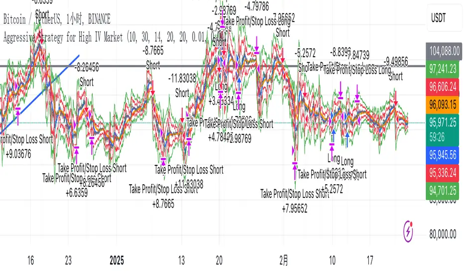
Aggressive Strategy for High IV Market### Strategic background
In a volatile high IV market, prices are volatile and market expectations of future uncertainty are high. This environment provides opportunities for aggressive trading strategies, but also comes with a high level of risk. In pursuit of a high Sharpe ratio (i.e., risk-adjusted return), we need to design a strategy that captures the benefits of market volatility while effectively controlling risk. Based on daily line cycles, I choose a combination of trend tracking and volatility filtering for highly volatile assets such as stocks, futures or cryptocurrencies.
---
### Strategy framework
#### Data
- Use daily data, including opening, closing, high and low prices.
- Suitable for highly volatile markets such as technology stocks, cryptocurrencies or volatile index futures.
#### Core indicators
1. ** Trend Indicators ** :
Fast Exponential Moving Average (EMA_fast) : 10-day EMA, used to capture short-term trends.
- Slow Exponential Moving Average (EMA_slow) : 30-day EMA, used to determine the long-term trend.
2. ** Volatility Indicators ** :
Average true Volatility (ATR) : 14-day ATR, used to measure market volatility.
- ATR mean (ATR_mean) : A simple moving average of the 20-day ATR that serves as a volatility benchmark.
- ATR standard deviation (ATR_std) : The standard deviation of the 20-day ATR, which is used to judge extreme changes in volatility.
#### Trading logic
The strategy is based on a trend following approach of double moving averages and filters volatility through ATR indicators, ensuring that trading only in a high-volatility environment is in line with aggressive and high sharpe ratio goals.
---
### Entry and exit conditions
#### Admission conditions
- ** Multiple entry ** :
- EMA_fast Crosses EMA_slow (gold cross), indicating that the short-term trend is turning upward.
-ATR > ATR_mean + 1 * ATR_std indicates that the current volatility is above average and the market is in a state of high volatility.
- ** Short Entry ** :
- EMA_fast Crosses EMA_slow (dead cross) downward, indicating that the short-term trend turns downward.
-ATR > ATR_mean + 1 * ATR_std, confirming high volatility.
#### Appearance conditions
- ** Long show ** :
- EMA_fast Enters the EMA_slow (dead cross) downward, and the trend reverses.
- or ATR < ATR_mean-1 * ATR_std, volatility decreases significantly and the market calms down.
- ** Bear out ** :
- EMA_fast Crosses the EMA_slow (gold cross) on the top, and the trend reverses.
- or ATR < ATR_mean-1 * ATR_std, the volatility is reduced.
---
### Risk management
To control the high risk associated with aggressive strategies, set up the following mechanisms:
1. ** Stop loss ** :
- Long: Entry price - 2 * ATR.
- Short: Entry price + 2 * ATR.
- Dynamic stop loss based on ATR can adapt to market volatility changes.
2. ** Stop profit ** :
- Fixed profit target can be selected (e.g. entry price ± 4 * ATR).
- Or use trailing stop losses to lock in profits following price movements.
3. ** Location Management ** :
- Reduce positions appropriately in times of high volatility, such as dynamically adjusting position size according to ATR, ensuring that the risk of a single trade does not exceed 1%-2% of the account capital.
---
### Strategy features
- ** Aggressiveness ** : By trading only in a high ATR environment, the strategy takes full advantage of market volatility and pursues greater returns.
- ** High Sharpe ratio potential ** : Trend tracking combined with volatility filtering to avoid ineffective trades during periods of low volatility and improve the ratio of return to risk.
- ** Daily line Cycle ** : Based on daily line data, suitable for traders who operate frequently but are not too complex.
---
### Implementation steps
1. ** Data Preparation ** :
- Get the daily data of the target asset.
- Calculate EMA_fast (10 days), EMA_slow (30 days), ATR (14 days), ATR_mean (20 days), and ATR_std (20 days).
2. ** Signal generation ** :
- Check EMA cross signals and ATR conditions daily to generate long/short signals.
3. ** Execute trades ** :
- Enter according to the signal, set stop loss and profit.
- Monitor exit conditions and close positions in time.
4. ** Backtest and Optimization ** :
- Use historical data to backtest strategies to evaluate Sharpe ratios, maximum retracements, and win rates.
- Optimize parameters such as EMA period and ATR threshold to improve policy performance.
---
### Precautions
- ** Trading costs ** : Highly volatile markets may result in frequent trading, and the impact of fees and slippage on earnings needs to be considered.
- ** Risk Control ** : Aggressive strategies may face large retracements and need to strictly implement stop losses.
- ** Scalability ** : Additional metrics (such as volume or VIX) can be added to enhance strategy robustness, or combined with machine learning to predict trends and volatility.
---
### Summary
This is a trend following strategy based on dual moving averages and ATR, designed for volatile high IV markets. By entering into high volatility and exiting into low volatility, the strategy combines aggressive and risk-adjusted returns for traders seeking a high sharpe ratio. It is recommended to fully backtest before implementation and adjust the parameters according to the specific market.
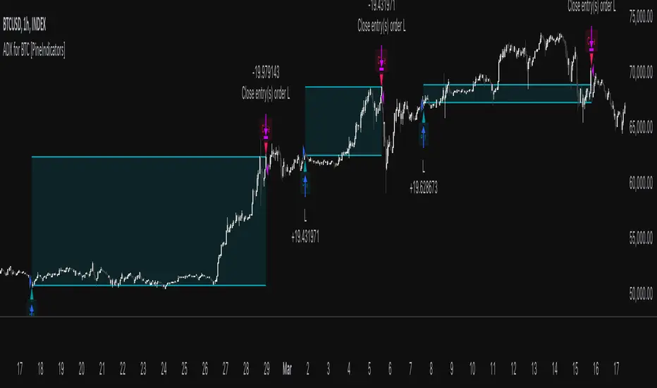
ADX for BTC [PineIndicators]The ADX Strategy for BTC is a trend-following system that uses the Average Directional Index (ADX) to determine market strength and momentum shifts. Designed for Bitcoin trading, this strategy applies a customizable ADX threshold to confirm trend signals and optionally filters entries using a Simple Moving Average (SMA). The system features automated entry and exit conditions, dynamic trade visualization, and built-in trade tracking for historical performance analysis.
⚙️ Core Strategy Components
1️⃣ Average Directional Index (ADX) Calculation
The ADX indicator measures trend strength without indicating direction. It is derived from the Positive Directional Movement (+DI) and Negative Directional Movement (-DI):
+DI (Positive Directional Index): Measures upward price movement.
-DI (Negative Directional Index): Measures downward price movement.
ADX Value: Higher values indicate stronger trends, regardless of direction.
This strategy uses a default ADX length of 14 to smooth out short-term fluctuations while detecting sustainable trends.
2️⃣ SMA Filter (Optional Trend Confirmation)
The strategy includes a 200-period SMA filter to validate trend direction before entering trades. If enabled:
✅ Long Entry is only allowed when price is above a long-term SMA multiplier (5x the standard SMA length).
✅ If disabled, the strategy only considers the ADX crossover threshold for trade entries.
This filter helps reduce entries in sideways or weak-trend conditions, improving signal reliability.
📌 Trade Logic & Conditions
🔹 Long Entry Conditions
A buy signal is triggered when:
✅ ADX crosses above the threshold (default = 14), indicating a strengthening trend.
✅ (If SMA filter is enabled) Price is above the long-term SMA multiplier.
🔻 Exit Conditions
A position is closed when:
✅ ADX crosses below the stop threshold (default = 45), signaling trend weakening.
By adjusting the entry and exit ADX levels, traders can fine-tune sensitivity to trend changes.
📏 Trade Visualization & Tracking
Trade Markers
"Buy" label (▲) appears when a long position is opened.
"Close" label (▼) appears when a position is exited.
Trade History Boxes
Green if a trade is profitable.
Red if a trade closes at a loss.
Trend Tracking Lines
Horizontal lines mark entry and exit prices.
A filled trade box visually represents trade duration and profitability.
These elements provide clear visual insights into trade execution and performance.
⚡ How to Use This Strategy
1️⃣ Apply the script to a BTC chart in TradingView.
2️⃣ Adjust ADX entry/exit levels based on trend sensitivity.
3️⃣ Enable or disable the SMA filter for trend confirmation.
4️⃣ Backtest performance to analyze historical trade execution.
5️⃣ Monitor trade markers and history boxes for real-time trend insights.
This strategy is designed for trend traders looking to capture high-momentum market conditions while filtering out weak trends.
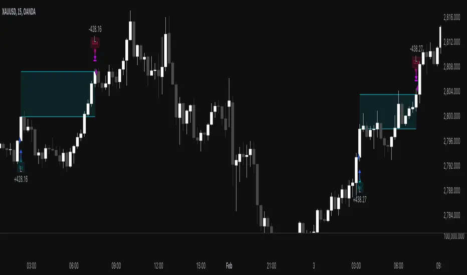
MACD Volume Strategy for XAUUSD (15m) [PineIndicators]The MACD Volume Strategy is a momentum-based trading system designed for XAUUSD on the 15-minute timeframe. It integrates two key market indicators: the Moving Average Convergence Divergence (MACD) and a volume-based oscillator to identify strong trend shifts and confirm trade opportunities. This strategy uses dynamic position sizing, incorporates leverage customization, and applies structured entry and exit conditions to improve risk management.
⚙️ Core Strategy Components
1️⃣ Volume-Based Momentum Calculation
The strategy includes a custom volume oscillator to filter trade signals based on market activity. The oscillator is derived from the difference between short-term and long-term volume trends using Exponential Moving Averages (EMAs)
Short EMA (default = 5) represents recent volume activity.
Long EMA (default = 8) captures broader volume trends.
Positive values indicate rising volume, supporting momentum-based trades.
Negative values suggest weak market activity, reducing signal reliability.
By requiring positive oscillator values, the strategy ensures momentum confirmation before entering trades.
2️⃣ MACD Trend Confirmation
The strategy uses the MACD indicator as a trend filter. The MACD is calculated as:
Fast EMA (16-period) detects short-term price trends.
Slow EMA (26-period) smooths out price fluctuations to define the overall trend.
Signal Line (9-period EMA) helps identify crossovers, signaling potential trend shifts.
Histogram (MACD – Signal) visualizes trend strength.
The system generates trade signals based on MACD crossovers around the zero line, confirming bullish or bearish trend shifts.
📌 Trade Logic & Conditions
🔹 Long Entry Conditions
A buy signal is triggered when all the following conditions are met:
✅ MACD crosses above 0, signaling bullish momentum.
✅ Volume oscillator is positive, confirming increased trading activity.
✅ Current volume is at least 50% of the previous candle’s volume, ensuring market participation.
🔻 Short Entry Conditions
A sell signal is generated when:
✅ MACD crosses below 0, indicating bearish momentum.
✅ Volume oscillator is positive, ensuring market activity is sufficient.
✅ Current volume is less than 50% of the previous candle’s volume, showing decreasing participation.
This multi-factor approach filters out weak or false signals, ensuring that trades align with both momentum and volume dynamics.
📏 Position Sizing & Leverage
Dynamic Position Calculation:
Qty = strategy.equity × leverage / close price
Leverage: Customizable (default = 1x), allowing traders to adjust risk exposure.
Adaptive Sizing: The strategy scales position sizes based on account equity and market price.
Slippage & Commission: Built-in slippage (2 points) and commission (0.01%) settings provide realistic backtesting results.
This ensures efficient capital allocation, preventing overexposure in volatile conditions.
🎯 Trade Management & Exits
Take Profit & Stop Loss Mechanism
Each position includes predefined profit and loss targets:
Take Profit: +10% of risk amount.
Stop Loss: Fixed at 10,100 points.
The risk-reward ratio remains balanced, aiming for controlled drawdowns while maximizing trade potential.
Visual Trade Tracking
To improve trade analysis, the strategy includes:
📌 Trade Markers:
"Buy" label when a long position opens.
"Close" label when a position exits.
📌 Trade History Boxes:
Green for profitable trades.
Red for losing trades.
📌 Horizontal Trade Lines:
Shows entry and exit prices.
Helps identify trend movements over multiple trades.
This structured visualization allows traders to analyze past performance directly on the chart.
⚡ How to Use This Strategy
1️⃣ Apply the script to a XAUUSD (Gold) 15m chart in TradingView.
2️⃣ Adjust leverage settings as needed.
3️⃣ Enable backtesting to assess past performance.
4️⃣ Monitor volume and MACD conditions to understand trade triggers.
5️⃣ Use the visual trade markers to review historical performance.
The MACD Volume Strategy is designed for short-term trading, aiming to capture momentum-driven opportunities while filtering out weak signals using volume confirmation.
Hanzo_Wave_Price %Hanzo_Wave_Price % is a custom indicator for the TradingView platform that combines RSI (Relative Strength Index) and Stochastic RSI while also displaying the percentage price change over a specified period. This indicator helps traders identify overbought and oversold conditions, analyze price waves, and forecast potential market movements.
How It Works
1. RSI and Stochastic RSI Calculation
RSI is calculated based on the selected price source (default: close) with a user-defined Main Line period.
Stochastic RSI is then applied and smoothed using a moving average.
The Main Line represents the smoothed Stochastic RSI, serving as a wave indicator to help identify potential entry and exit points.
2. Overbought and Oversold Zones
The 70 and 30 levels indicate overbought and oversold zones, displayed as dashed lines on the chart.
Additional 20% and 10% levels provide a visual reference for historical price changes, aiding in future predictions.
3. Percentage Price Change Calculation
The indicator calculates the percentage price change over a Barsback period (default: 30 candles).
Users can choose a multiplier (100 or 1000) for better visualization (1000 scales the values by dividing by 10).
The data is displayed as a colored area:
Red (Short) → Negative price change.
Green (Buy) → Positive price change.
Settings & Parameters
Multiplier 💪 – Selects the scaling factor (100 or 1000) for percentage values.
Main Line ✈️ – Stochastic smoothing period (smoothK).
Don't touch ✋ – Reserved value (do not modify).
RSI 🔴 – RSI calculation period.
Stochastic 🔵 – Stochastic RSI calculation period.
Source ⚠️ – Price source for calculations (default: close).
Price changes % 🔼🔽 – Enables percentage price change display.
Barsback ↩️ – Number of candles used to calculate price change.
Visual Representation
Gray Line (Takeprofit Line 🎯) – Smoothed Stochastic RSI.
Red Dashed Line (70) – Overbought zone.
Blue Dashed Line (30) – Oversold zone.
Percentage Price Change Display:
Green Fill → Price increase.
Red Fill → Price decrease.
Advantages
✅ Combined Analysis – Uses RSI and Stochastic RSI for more accurate market condition identification.
✅ Flexibility – Customizable parameters allow adaptation for different markets and strategies.
✅ Visual Clarity – Clearly defined zones and dynamic percentage change display.
✅ Additional Market Insights – The percentage price change helps assess market volatility.
Disadvantages
⚠ Lagging Signals – Smoothing may cause delayed response.
⚠ False Breakouts – The 70/30 levels may not always work effectively for all assets.
⚠ IMPORTANT!
This indicator is for informational and educational purposes only. Past performance does not guarantee future profits! Use it in combination with other technical analysis tools. 🚀
Example 1: Identifying a Long Position
📌 Scenario:
The asset price has dropped significantly (1-hour timeframe), and the Main Line (gray line) crosses below the 30 level. This signals oversold conditions, which may indicate a potential reversal or upward correction.
✅ How to Use:
1️⃣ Identifying the Entry Zone:
If the Main Line is below 30, consider looking for a long entry point.
2️⃣ Confirming the Signal:
Place a vertical line at the moment when the Main Line crosses the 30 level from below.
3️⃣ Confirmation on a Lower Timeframe:
Switch to a 30-minute timeframe and wait for the Main Line to cross above the 70 level.
Enter a long position at this point.
4️⃣ Analyzing Percentage Price Change:
Check the historical indicator behavior:
If a similar past movement resulted in a ~10% price increase (green fill), this may indicate potential upward momentum.
5️⃣ Setting Take-Profit:
Set a take-profit level at 10%, based on previous price movements.
Also, monitor when the Main Line crosses the 70 level, as this may signal a potential profit-taking point.
📊 Conclusion:
This method helps to precisely determine entry points by confirming signals across multiple timeframes and analyzing the historical volatility of the asset. 🚀
Example 2: Analyzing Percentage Price Change
📌 Scenario:
You have set the Barsback parameter to 30, and the indicator shows +3.5%. This means that over the last 30 candles, the price has increased by 3.5%.
However, such small changes might be visually difficult to notice. To improve visibility, you can enable the multiplier (1000), which will scale the displayed percentage change to 35%. This is purely for visual convenience—the actual price movement remains 3.5%.
✅ How to Use:
1️⃣ Identifying Trend Direction:
If the percentage change is positive (green area) → Uptrend.
If the percentage change is negative (red area) → Downtrend.
2️⃣ Analyzing Movement Strength:
Compare the current percentage change with previous waves to evaluate the strength of the movement.
For example:
If previous waves reached 10% or more, a current wave of 3.5% might indicate a weak trend or a local correction.
3️⃣ Additional Filtering with the Main Line (Gray Line):
Use the Main Line to confirm the trend.
If the percentage change shows an increase, but the Main Line is still below 30, further upward movement can be expected.
If the percentage change indicates a decline, but the Main Line is above 70, there is a higher probability of a downward reversal.
"It's unfortunate that TradingView restricts adding images to indicator descriptions unless you have a paid subscription. This makes it harder to share free tools effectively."

Pivot Candles with MFI Opacity (No Plot)How to Use the Pivot Candles with MFI Opacity Indicator for Trade Entries and Position Management
Overview
This indicator is designed not only to display key pivot levels (support and resistance) and Money Flow Index (MFI) signals on your chart, but also to help you structure systematic order entries and position management. By combining pivot levels with dynamic MFI-based candle opacity, the indicator provides a visual framework that technical analysts and quants can use to time buy and sell stop orders as well as to pyramid positions or take profits.
Trade Entry with Pivot Levels
Buy Stop Orders Above R1:
Concept: In many technical setups, resistance levels such as R1 are viewed as potential breakout points. A buy stop order placed just above R1 allows you to enter a long position only when price decisively breaks the prior resistance, confirming bullish momentum.
How It Works:
The indicator calculates pivot levels based on the previous higher‑timeframe bar, so R1 is “locked in” for the current period.
When the current candle closes above R1, it may signal a breakout.
Technical analysts often place a buy stop order slightly above R1 (for example, a few ticks or pips above the level) to confirm the move.
Practical Application:
Quants and systematic traders can program their models to monitor when the current close exceeds R1.
Once this condition is met, a buy stop order is triggered to capture the breakout move, ensuring that you only participate if the price decisively moves upward.
Sell Stop Orders Below S1:
Concept: Conversely, S1 acts as a support level. A sell stop order placed just below S1 is designed to capture a breakdown. This order is activated when price closes below S1, indicating that selling pressure may be overwhelming.
How It Works:
With pivot levels fixed from the previous higher‑timeframe bar, S1 provides a reference for potential support.
A close below S1 can be interpreted as a sign of a bearish reversal or a continuation of a downtrend.
Practical Application:
Quants set up their systems to watch for a break below S1.
A sell stop order is positioned just below S1 to ensure that if the support level fails, the system can quickly initiate a short position to capture the downward move.
Using MFI for Position Management
Pyramiding and Profit Taking:
Dynamic Candle Opacity:
The Money Flow Index (MFI) in this indicator not only provides overbought/oversold alerts but also controls the opacity of your candlesticks. When MFI readings are high, the candles become more opaque, indicating strong buying pressure. Conversely, lower MFI values lead to more transparent candles, suggesting reduced momentum.
Pyramiding Long Positions:
Strategy:
In a strong trend, technical analysts might choose to add to a winning position gradually—a process known as pyramiding.
Implementation:
As long as the price remains above R1 and MFI readings are supportive (high and consistent), you may consider adding to your long position incrementally.
Each new buy stop order can be set above R1 with slightly adjusted trigger levels to capture further breakout strength.
Risk Management:
Quants use the MFI reading as a risk filter; if MFI begins to drop or the candles become significantly more transparent, it may be a cue to stop pyramiding or even begin taking profits.
Taking Profit Using MFI and Pivot Reversals:
Profit Targeting:
When price reaches higher resistance levels (e.g., R2 or R3) or shows signs of overextension in conjunction with extreme MFI levels (for instance, a sudden drop in MFI after a strong rally), you can begin taking partial profits.
Systematic Exit:
A systematic strategy might include scaling out of the position as the price approaches the next resistance level or when the MFI indicates that buying momentum is waning.
Similarly, for short positions entered below S1, profit targets might be set near subsequent support levels, with exits triggered if MFI suggests a reversal.
Summary
Entry Orders:
Place buy stop orders just above R1 to capture breakouts.
Place sell stop orders just below S1 to capture breakdowns.
Position Management with MFI:
Use MFI-based candle opacity as a visual indicator of momentum.
Pyramid positions in the direction of the trend when MFI confirms strength.
Consider partial exits if MFI readings start to reverse or if the price nears the next pivot level.
By following this systematic approach, technical analysts and quants can use the indicator not only as a visual tool but as an integral part of an automated or semi-automated trading system that emphasizes disciplined entries, pyramiding, and profit-taking.

2xSPYTIPS Strategy by Fra public versionThis is a test strategy with S&P500, open source so everyone can suggest everything, I'm open to any advice.
Rules of the "2xSPYTIPS" Strategy :
This trading strategy is designed to operate on the S&P 500 index and the TIPS ETF. Here’s how it works:
1. Buy Conditions ("BUY"):
- The S&P 500 must be above its **200-day simple moving average (SMA 200)**.
- This condition is checked at the **end of each month**.
2. Position Management:
- If leverage is enabled (**2x leverage**), the purchase quantity is increased based on a configurable percentage.
3. Take Profit:
- A **Take Profit** is set at a fixed percentage above the entry price.
4. Visualization & Alerts:
- The **SMA 200** for both S&P 500 and TIPS is plotted on the chart.
- A **BUY signal** appears visually and an alert is triggered.
What This Strategy Does NOT Do
- It does not use a **Stop Loss** or **Trailing Stop**.
- It does not directly manage position exits except through Take Profit.

AdvancedLines (FiboBands) - PaSKaL
Overview :
AdvancedLines (FiboBands) - PaSKaL is an advanced technical analysis tool designed to automate the plotting of key Fibonacci retracement levels based on the highest high and lowest low over a customizable period. This indicator helps traders identify critical price zones such as support, resistance, and potential trend reversal or continuation points.
By using AdvancedLines (FiboBands) - PaSKaL , traders can easily spot key areas where the price is likely to reverse or consolidate, or where the trend may continue. It is particularly useful for trend-following, scalping, and range-trading strategies.
Key Features:
Automatic Fibonacci Level Calculation :
- The indicator automatically calculates and plots key Fibonacci levels (0.236, 0.382, 0.5, 0.618, and 0.764), which are crucial for identifying potential support and resistance levels in the market.
Adjustable Parameters :
- Bands Length: You can adjust the bands_length setting to change the number of bars used for calculating the highest high and lowest low. This gives flexibility for using the indicator on different timeframes and trading styles.
- Visibility: The Fibonacci levels, as well as the midline (0.5 Fibonacci level), can be shown or hidden based on your preference.
- Color Customization: You can change the color of each Fibonacci level and background fills to suit your chart preferences.
Fibonacci Levels
- The main Fibonacci levels plotted are:
- 0.236 – Minor support/resistance level
- 0.382 – Moderate retracement level
- 0.5 – Midpoint retracement, often used as a key level
- 0.618 – Golden ratio, considered one of the most important Fibonacci levels
- 0.764 – Strong reversal level, often indicating a continuation or change in trend
Background Fill
- The indicator allows you to fill the background between the Fibonacci levels and the bands with customizable colors. This makes it easier to visually highlight key zones on the chart.
How the Indicator Works:
AdvancedLines (FiboBands) - PaSKaL calculates the range (difference between the highest high and the lowest low) over a user-defined number of bars (e.g., 300). Fibonacci levels are derived from this range, helping traders identify potential price reversal points.
Mathematical Basis :
Fibonacci retracement levels are based on the Fibonacci sequence, where each number is the sum of the previous two (0, 1, 1, 2, 3, 5, 8, 13, etc.). The ratios derived from this sequence (such as 0.618 and 0.382) have been widely observed in nature, market cycles, and price movements. These ratios are used to forecast potential price retracements or continuation points after a major price move.
Fibonacci Levels Calculation :
Identify the Range: The highest high and the lowest low over the defined period are calculated.
Apply Fibonacci Ratios: Fibonacci ratios (0.236, 0.382, 0.5, 0.618, and 0.764) are applied to this range to calculate the corresponding price levels.
Plot the Levels: The indicator automatically plots these levels on your chart.
Customizing Fibonacci Levels & Colors:
The "AdvancedLines (FiboBands) - PaSKaL" indicator offers various customization options for Fibonacci levels, colors, and visibility:
Fibonacci Level Ratios:
- You can customize the Fibonacci level ratios through the following inputs:
- Fibo Level 1: 0.764
- Fibo Level 2: 0.618
- Fibo Level 3: 0.5
- Fibo Level 4: 0.382
- Fibo Level 5: 0.236
- These levels determine key areas where price may reverse or pause. You can adjust these ratios based on your trading preferences.
Fibonacci Level Colors:
- Each Fibonacci level can be assigned a different color to make it more distinguishable on your chart:
- Fibo Level 1 Color (default: Yellow)
- Fibo Level 2 Color (default: Orange)
- Fibo Level 3 Color (default: Green)
- Fibo Level 4 Color (default: Red)
- Fibo Level 5 Color (default: Blue)
- You can change these colors to fit your visual preferences or to align with your existing chart themes.
Visibility of Fibonacci Levels:
- You can choose whether to display each Fibonacci level using the following visibility inputs:
- Show Fibo Level 1 (0.764): Display or hide this level.
- Show Fibo Level 2 (0.618): Display or hide this level.
- Show Fibo Level 3 (0.5): Display or hide this level.
- Show Fibo Level 4 (0.382): Display or hide this level.
- Show Fibo Level 5 (0.236): Display or hide this level.
- This allows you to customize the indicator according to the specific Fibonacci levels that are most relevant to your trading strategy.
Background Fill Color
- The background between the Fibonacci levels and price bands can be filled with customizable colors:
- Fill Color for Upper Band & Fibo Level 1: This color will fill the area between the upper band and Fibonacci Level 1.
- Fill Color for Lower Band & Fibo Level 5: This color will fill the area between the lower band and Fibonacci Level 5.
- Adjusting these colors helps highlight critical zones where price may reverse or consolidate.
How to Use AdvancedLines (FiboBands) - PaSKaL in Trading :
Range Trading :
Range traders typically buy at support and sell at resistance. Fibonacci levels provide excellent support and resistance zones in a ranging market.
Example: If price reaches the 0.618 level in an uptrend, it may reverse, providing an opportunity to sell.
Conversely, if price drops to the 0.382 level, a bounce might occur, and traders can buy, anticipating the market will stay within the range.
Trend-following Trading :
For trend-following traders, Fibonacci levels act as potential entry points during a retracement. After a strong trend, price often retraces to one of the Fibonacci levels before continuing in the direction of the trend.
Example: In a bullish trend, when price retraces to the 0.382 level, it could be a signal to buy, as the price might resume its upward movement after the correction.
In a bearish trend, retracements to levels like 0.618 or 0.764 could provide optimal opportunities for shorting as the price resumes its downward movement.
Scalping :
Scalpers focus on short-term price movements. Fibonacci levels can help identify precise entry and exit points for quick trades.
Example: If price is fluctuating in a narrow range, a scalper can enter a buy trade at 0.236 and exit at the next Fibonacci level, such as 0.382 or 0.5, capturing small but consistent profits.
Stop-Loss and Take-Profit Levels :
Fibonacci levels can also help in setting stop-loss and take-profit levels.
Example: In a bullish trend, you can set a stop-loss just below the 0.236 level and a take-profit at 0.618.
In a bearish trend, set the stop-loss just above the 0.382 level and the take-profit at 0.764.
Identifying Reversals and Continuations :
Reversals: When price reaches a Fibonacci level and reverses direction, it may indicate the end of a price move.
Trend Continuation: If price bounces off a Fibonacci level and continues in the same direction, this may signal that the trend is still intact.
Conclusion :
AdvancedLines (FiboBands) - PaSKaL is an essential tool for any trader who uses Fibonacci retracements in their trading strategy. By automatically plotting key Fibonacci levels, this indicator helps traders quickly identify support and resistance zones, forecast potential reversals, and make more informed trading decisions.
For Trend-following Traders: Use Fibonacci levels to find optimal entry points after a price retracement.
For Range Traders: Identify key levels where price is likely to reverse or bounce within a range.
For Scalpers: Pinpoint small price movements and take advantage of quick profits by entering and exiting trades at precise Fibonacci levels.
By incorporating AdvancedLines (FiboBands) - PaSKaL into your trading setup, you will gain a deeper understanding of price action, improve your decision-making process, and enhance your overall trading performance.

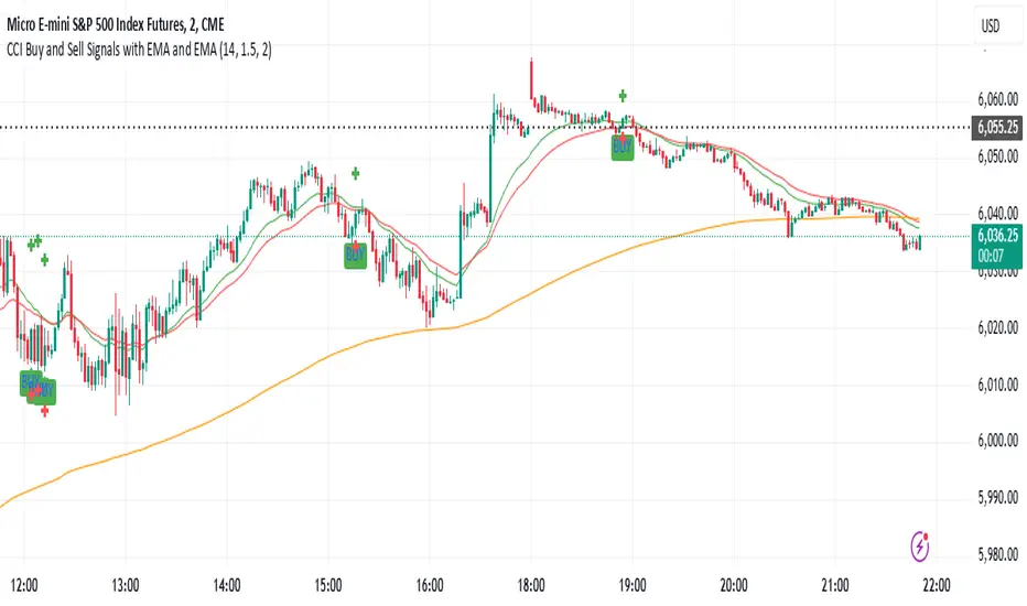
CCI Buy and Sell Signals with 20/30 EMACCI Buy and Sell Signals with EMA and ATR Stop Loss/Take Profit
This indicator is designed to identify buy and sell signals based on a combination of the Commodity Channel Index (CCI) and Exponential Moving Averages (EMA). It also includes an optional ATR-based stop loss and take profit system, which is useful for traders who want to manage their trades with dynamic risk levels.
Features:
CCI Buy and Sell Signals:
Buy Signal: A buy signal is triggered when the CCI crosses up through -100 (from an oversold condition), the 20-period EMA is above the 30-period EMA, and the price is above the 200-period EMA. This suggests that the market is entering an upward trend.
Sell Signal: A sell signal is triggered when the CCI crosses down through +100 (from an overbought condition), the 20-period EMA is below the 30-period EMA, and the price is below the 200-period EMA. This suggests that the market is entering a downward trend.
Exponential Moving Averages (EMA):
The script plots three EMAs:
20-period EMA (Green): Used to identify short-term trends.
30-period EMA (Red): Used to capture medium-term trends.
200-period EMA (Orange): A long-term trend filter, with the price above it generally indicating bullish conditions and below it indicating bearish conditions.
ATR-Based Stop Loss and Take Profit:
Optional Feature: The ATR (Average True Range) indicator can be used to set stop loss and take profit levels based on market volatility.
Stop Loss: Set at a multiple of the ATR below the entry price for long positions and above the entry price for short positions.
Take Profit: Set at a multiple of the ATR above the entry price for long positions and below the entry price for short positions.
Customizable: You can adjust the ATR length, Stop Loss Multiplier, and Take Profit Multiplier through the settings.
Dots: The stop loss and take profit levels are plotted as dots on the chart when the ATR feature is enabled.
Alert Conditions:
Buy Signal Alert: Triggered when a buy signal occurs based on CCI crossing up -100 and other conditions being met.
Sell Signal Alert: Triggered when a sell signal occurs based on CCI crossing down +100 and other conditions being met.
Any Signal Alert: This is a combined alert that triggers for either a buy or sell signal. It helps you stay updated on both types of signals simultaneously.
How to Use:
The indicator will plot buy and sell arrows on the chart, giving clear entry points for trades based on CCI and EMA conditions.
The ATR stop loss and take profit dots (when enabled) provide automatic risk management levels, adjusting dynamically with market volatility.
Traders can customize the ATR settings to fine-tune their stop loss and take profit levels, making this strategy adaptable to different trading styles and market conditions.
Reversal rehersal v1This indicator was designed to identify potential market reversal zones using a combination of RSI thresholds (shooting range/falling range), candlestick patterns, and Fair Value Gaps (FVGs). By combining all these elements into one indicator, it allow for outputting high probability buy/sell signals for use by scalpers on low timeframes like 1-15 mins, for quick but small profits.
Note: that this has been mainly tested on DE40 index on the 1 min timeframe, and need to be adjusted to whichever timeframe and symbol you intend to use. Refer to the backtester feature for checking if this indicator may work for you.
The indicator use RSI ranges from two timeframes to highlight where momentum is building up. During these areas, it will look for certain candlestick patterns (Sweeps as the primary one) and check for existance of fair value gaps to further enhance the hitrate of the signal.
The logic for FVG detection was based on ©pmk07's work with MTF FVG tiny indicator. Several major changes was implemented though and incorporated into this indicator. Among these are:
Automatically adjustments of FVG boxes when mitigated partially and options to extend/cull boxes for performance and clarity.
Backtesting Table (Experimental):
This indicator also features an optional simplified table to review historical theoretical performance of signals, including win rate, profit/loss, and trade statistics. This does not take commision or slippage into consideration.
Usage Notes:
Setup:
1. Add the indicator to your chart.
2. Decide if you want to use Long or Short (or both).
3. If you're scalping on ie. 1 min time frame, make sure to set FVG's to higher timeframes (ie. 5, 15, 60).
4. Enable the 'Show backtest results' and adjust the 'Signals' og 'Take profit' and 'Stop loss' values until you are satisfied with the results.
Use:
1. Setup an alert based on either of the 'BullishShooting range' or 'BearishFalling range' alerts. This will draw your attention to watch for the possible setups.
2. Verify if there's a significant imbalance prior to the signal before taking the trade. Otherwise this may invalidate the setup.
3. Once a signal is shown on the graph (either Green arrow up for buys/Red arrow down for sells) - you should enter a trade with the given 'Take profit' and 'Stop loss' values.
4. (optional) Setup an alert for either the Strong/Weak signals. Which corresponds to when one of the arrows are printed.
Important: This is the way I use it myself, but use at own risk and remember to combine with other indicators for further confluence. Remember this is no crystal ball and I do not guarantee profitable results. The indicator merely show signals with high probability setups for scalping.

SMA + RSI + Volume + ATR StrategySMA + RSI + Volume + ATR Strategy
1. Indicators Used:
SMA (Simple Moving Average): This is a trend-following indicator that calculates the average price of a security over a specified period (50 periods in this case). It's used to identify the overall trend of the market.
RSI (Relative Strength Index): This measures the speed and change of price movements. It tells us if the market is overbought (too high) or oversold (too low). Overbought is above 70 and oversold is below 30.
Volume: This is the amount of trading activity. A higher volume often indicates strong interest in a particular price move.
ATR (Average True Range): This measures volatility, or how much the price is moving in a given period. It helps us adjust stop losses and take profits based on market volatility.
2. Conditions for Entering Trades:
Buy Signal (Green Up Arrow):
Price is above the 50-period SMA (indicating an uptrend).
RSI is below 30 (indicating the market might be oversold or undervalued, signaling a potential reversal).
Current volume is higher than average volume (indicating strong interest in the move).
ATR is increasing (indicating higher volatility, suggesting that the market might be ready for a move).
Sell Signal (Red Down Arrow):
Price is below the 50-period SMA (indicating a downtrend).
RSI is above 70 (indicating the market might be overbought or overvalued, signaling a potential reversal).
Current volume is higher than average volume (indicating strong interest in the move).
ATR is increasing (indicating higher volatility, suggesting that the market might be ready for a move).
3. Take Profit & Stop Loss:
Take Profit: When a trade is made, the strategy will set a target price at a certain percentage above or below the entry price (1.5% in this case) to automatically exit the trade once that target is hit.
Stop Loss: If the price goes against the position, a stop loss is set at a percentage below or above the entry price (0.5% in this case) to limit losses.
4. Execution of Trades:
When the buy condition is met, the strategy will enter a long position (buying).
When the sell condition is met, the strategy will enter a short position (selling).
5. Visual Representation:
Green Up Arrow: Appears on the chart when the buy condition is met.
Red Down Arrow: Appears on the chart when the sell condition is met.
These arrows help you see at a glance when the strategy suggests you should buy or sell.
In Summary:
This strategy uses a combination of trend-following (SMA), momentum (RSI), volume, and volatility (ATR) to decide when to buy or sell a stock. It looks for opportunities when the market is either oversold (buy signal) or overbought (sell signal) and makes sure there’s enough volume and volatility to back up the move. It also includes take-profit and stop-loss levels to manage risk.

Bollinger Bands Reversal Strategy Analyzer█ OVERVIEW
The Bollinger Bands Reversal Overlay is a versatile trading tool designed to help traders identify potential reversal opportunities using Bollinger Bands. It provides visual signals, performance metrics, and a detailed table to analyze the effectiveness of reversal-based strategies over a user-defined lookback period.
█ KEY FEATURES
Bollinger Bands Calculation
The indicator calculates the standard Bollinger Bands, consisting of:
A middle band (basis) as the Simple Moving Average (SMA) of the closing price.
An upper band as the basis plus a multiple of the standard deviation.
A lower band as the basis minus a multiple of the standard deviation.
Users can customize the length of the Bollinger Bands and the multiplier for the standard deviation.
Reversal Signals
The indicator identifies potential reversal signals based on the interaction between the price and the Bollinger Bands.
Two entry strategies are available:
Revert Cross: Waits for the price to close back above the lower band (for longs) or below the upper band (for shorts) after crossing it.
Cross Threshold: Triggers a signal as soon as the price crosses the lower band (for longs) or the upper band (for shorts).
Trade Direction
Users can select a trade bias:
Long: Focuses on bullish reversal signals.
Short: Focuses on bearish reversal signals.
Performance Metrics
The indicator calculates and displays the performance of trades over a user-defined lookback period ( barLookback ).
Metrics include:
Win Rate: The percentage of trades that were profitable.
Mean Return: The average return across all trades.
Median Return: The median return across all trades.
These metrics are calculated for each bar in the lookback period, providing insights into the strategy's performance over time.
Visual Signals
The indicator plots buy and sell signals on the chart:
Buy Signals: Displayed as green triangles below the price bars.
Sell Signals: Displayed as red triangles above the price bars.
Performance Table
A customizable table is displayed on the chart, showing the performance metrics for each bar in the lookback period.
The table includes:
Win Rate: Highlighted with gradient colors (green for high win rates, red for low win rates).
Mean Return: Colored based on profitability (green for positive returns, red for negative returns).
Median Return: Colored similarly to the mean return.
Time Filtering
Users can define a specific time window for the indicator to analyze trades, ensuring that performance metrics are calculated only for the desired period.
Customizable Display
The table's font size can be adjusted to suit the user's preference, with options for "Auto," "Small," "Normal," and "Large."
█ PURPOSE
The Bollinger Bands Reversal Overlay is designed to:
Help traders identify high-probability reversal opportunities using Bollinger Bands.
Provide actionable insights into the performance of reversal-based strategies.
Enable users to backtest and optimize their trading strategies by analyzing historical performance metrics.
█ IDEAL USERS
Swing Traders: Looking for reversal opportunities within a trend.
Mean Reversion Traders: Interested in trading price reversals to the mean.
Strategy Developers: Seeking to backtest and refine Bollinger Bands-based strategies.
Performance Analysts: Wanting to evaluate the effectiveness of reversal signals over time.

ATR-Based Suitability CheckerPurpose:
This indicator helps traders identify the most suitable timeframe for trading by comparing fees to market volatility (ATR). Instead of filtering out specific assets or strategies, it focuses on finding optimal trading conditions for the selected timeframe. It is designed to adapt dynamically, ensuring that traders can align their approach with the current market environment.
Key Features:
Dynamic ATR Analysis: Measures volatility using the Average True Range (ATR) and evaluates how fees impact potential profitability across timeframes.
Fee-to-ATR Ratio: Calculates the proportion of fees to ATR, highlighting conditions where fees are too large relative to price movements.
Visual Feedback: **Red Background:** Indicates unsuitable trading conditions where fees dominate. **Green Background:** Highlights suitable conditions for trading efficiency. Markers provide quick visual identification of suitability.
Custom Transparency: Enables users to adjust the background’s transparency for better chart visibility.
How to Use:
Timeframe Optimization: When volatility rises, price movements become larger, making shorter timeframes more suitable for trading. Conversely, during periods of low volatility, longer timeframes are preferable to avoid overtrading within a narrow price range.
Spot & Leverage Trading: For spot trading, this tool identifies conditions where fees (e.g., 0.25%-0.3%) might excessively impact profitability. For instance, if ATR is comparable to fees, the trading environment may not be ideal. In leveraged trading, the indicator helps assess whether the current volatility supports your chosen leverage level, ensuring that leverage does not amplify undue risks.
Efficiency Focus: The indicator emphasizes finding a balance between market conditions and your trading strategy. Not all timeframes need to be "suitable" at all times; instead, it highlights the best opportunities based on current market dynamics. Utilize the suitability ratio across different timeframes to guide and adjust your trading strategies effectively.
Input Parameters:
ATR Length: Defines the period for ATR calculation (default: 14).
Fee Percentage (%): Trading fee as a percentage of the closing price (default: 0.1%).
Unsuitable Threshold (% of 1 ATR): Sets the maximum acceptable fee-to-ATR ratio for suitable conditions (default: 20%).
Background Transparency (0-100): Adjusts the opacity of the background highlight (default: 80).
Who Should Use This:
This tool is ideal for traders seeking to align their strategy with market conditions by finding the most suitable timeframe. It applies to both spot and leveraged markets, helping optimize efficiency while managing fees and volatility.
Notes:
The ATR-Based Suitability Checker is a supplementary tool. Combine it with other forms of analysis for comprehensive decision-making.
Regularly adjust the parameters to match your trading preferences and market conditions.