20-day High BreakoutOverview:
The 20-day High Breakout Indicator is a very simple yet powerful tool designed for traders seeking to capitalize on significant price movements in the stock market. This indicator identifies potential buy and sell signals based on a stock's 20-day high breakout levels, making it an essential addition to your trading strategy.
Key Features:
Swing Period Input: Customize the swing period to your preferred number of days, with a default of 20 days, allowing flexibility based on your trading style.
Trailing Stop Level: Automatically calculates the trailing stop level based on the highest high and lowest low within the defined swing period, helping to manage risk and lock in profits.
Buy and Sell Signals: Generates clear buy signals when the price crosses above the trailing stop level and sell signals when the price crosses below, enabling timely entries and exits.
Visual Indicators: Plots buy signals as green upward triangles below the bars and sell signals as red downward triangles above the bars, providing easy-to-interpret visual cues directly on the chart.
How It Works:
Resistance and Support Levels: The indicator calculates the highest high (resistance) and lowest low (support) over the defined swing period.
Swing Direction: It determines the market direction by comparing the current closing price to the previous resistance and support levels.
Trailing Stop Calculation: Depending on the market direction, the trailing stop level is set to either the support or resistance level.
Signal Generation: Buy and sell signals are generated based on the crossover of the closing price and the trailing stop level, filtered to ensure only valid signals are displayed.
Visual Representation: The trailing stop level is plotted as a line, and buy/sell signals are marked with respective shapes for easy identification.
Usage:
Trend Following: Ideal for traders looking to follow trends and catch significant breakouts in the stock price.
Risk Management: Helps in managing risk by providing a trailing stop level that adjusts with market movements.
Visual Clarity: The clear visual signals make it easy for traders to interpret and act upon the indicator's signals.
Add the 20-day High Breakout Indicator to your TradingView charts to enhance your trading strategy and gain an edge in identifying profitable trading opportunities.
Cerca negli script per "profit"

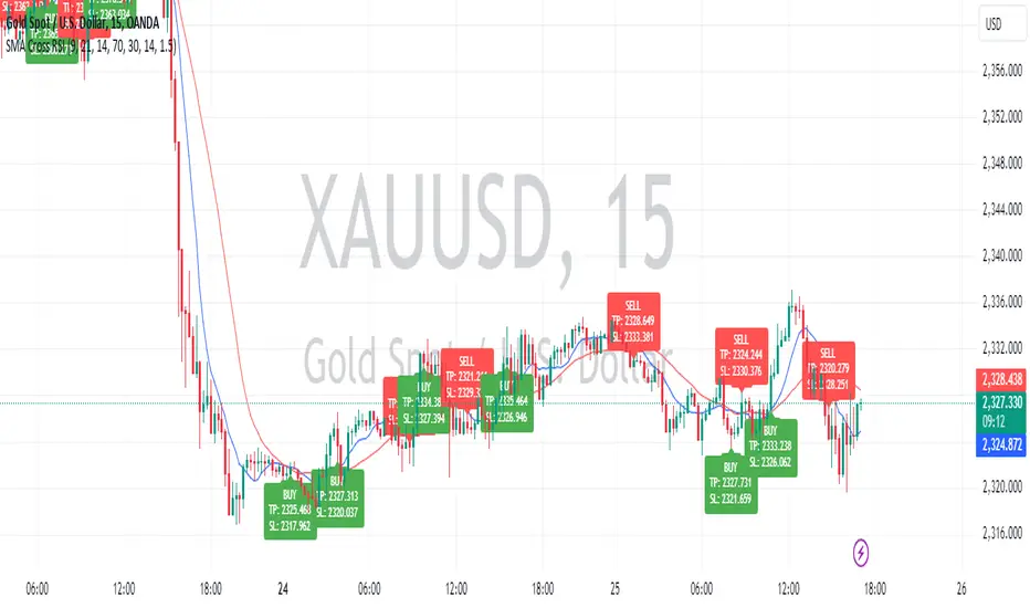
All Divergences with trend / SL - Uncle SamThanks to the main inspiration behind this strategy and the hard work of:
"Divergence for many indicators v4 by LonesomeTheBlue"
The "All Divergence" strategy is a versatile approach for identifying and acting upon various divergences in the market. Divergences occur when price and an indicator move in opposite directions, often signaling potential reversals. This strategy incorporates both regular and hidden divergences across multiple indicators (MACD, Stochastics, CCI, etc.) for a comprehensive analysis.
Key Features:
Comprehensive Divergence Analysis: The strategy scans for regular and hidden divergences across a variety of indicators, increasing the probability of identifying potential trade setups.
Trend Filter: To enhance accuracy, a moving average (MA) trend filter is integrated. This ensures trades align with the overall market trend, reducing the risk of false signals.
Customizable Risk Management: Users can adjust parameters for long/short stop-loss and take-profit levels to match their individual risk tolerance.
Additional Risk Management (Optional): An experimental MA-based risk management feature can be enabled to close positions if the market shows consecutive closes against the trend.
Clear Visuals: The script plots pivot points, divergence lines, and stop-loss levels on the chart for easy reference.
Strategy Settings (Defaults):
Enable Long/Short Strategy: True
Long/Short Stop Loss %: 2%
Long/Short Take Profit %: 5%
Enable MA Trend: True
MA Type: HMA (Hull Moving Average)
MA Length: 500
Use MA Risk Management: False (Experimental)
MA Risk Exit Candles: 2 (If enabled)
Pivot Period: 9
Source for Pivot Points: Close
Backtest Details (Example):
The strategy has been backtested on XAUUSD 1H (Goold/USD 1 hour timeframe) with a starting capital of $1,000. The backtest period covers around 2 years. A commission of 0.02% per trade and a 0.1% slippage per trade were factored in to simulate real-world trading costs.
Disclaimer:
This strategy is for educational and informational purposes only. Backtested results are not indicative of future performance. Use this strategy at your own risk. Always conduct your own analysis and consider consulting a financial professional before making any trading decisions.
Important Notes:
The default settings are a good starting point, but feel free to experiment to find optimal parameters for your specific trading style and market.
The MA-based risk management is an experimental feature. Use it with caution and thoroughly test it before deploying in live trading.
Backtest results can vary depending on the market, timeframe, and specific settings used. Always consider slippage and commission fees when evaluating a strategy's potential profitability.

Smoothed Heiken Ashi Strategy Long OnlyThis is a trend-following approach that uses a modified version of Heiken Ashi candles with additional smoothing. Here are the key components and features:
1. Heiken Ashi Modification: The strategy starts by calculating Heiken Ashi candles, which are known for better trend visualization. However, it modifies the traditional Heiken Ashi by using Exponential Moving Averages (EMAs) of the open, high, low, and close prices.
2. Double Smoothing: The strategy applies two layers of smoothing. First, it uses EMAs to calculate the Heiken Ashi values. Then, it applies another EMA to the Heiken Ashi open and close prices. This double smoothing aims to reduce noise and provide clearer trend signals.
3. Long-Only Approach: As the name suggests, this strategy only takes long positions. It doesn't short the market during downtrends but instead exits existing long positions when the sell signal is triggered.
4. Entry and Exit Conditions:
- Entry (Buy): When the smoothed Heiken Ashi candle color changes from red to green (indicating a potential start of an uptrend).
- Exit (Sell): When the smoothed Heiken Ashi candle color changes from green to red (indicating a potential end of an uptrend).
5. Position Sizing: The strategy uses a percentage of equity for position sizing, defaulting to 100% of available equity per trade. This should be tailored to each persons unique approach. Responsible trading would use less than 5% for each trade. The starting capital used is a responsible and conservative $1000, reflecting the average trader.
This strategy aims to provide a smooth, trend-following approach that may be particularly useful in markets with clear, sustained trends. However, it may lag in choppy or ranging markets due to its heavy smoothing. As with any strategy, it's important to thoroughly backtest and forward test before using it with real capital, and to consider using it in conjunction with other analysis tools and risk management techniques.
This has been created mainly to provide data to judge what time frame is most profitable for any single asset, as the volatility of each asset is different. This can bee seen using it on AUXUSD, which has a higher profitable result on the daily time frame, whereas other currencies need a higher or lower time frame. The user can toggle between each time frame and watch for the higher profit results within the strategy tester window.
Other smoothed Heiken Ashi indicators also do not provide buy and sell signals, and only show the change in color to dictate a change in trend. By adding buy and sell signals after the close of the candle in which the candle changes color, alerts can be programmed, which helps this be a more hands off protocol to experiment with. Other smoothed Heiken Ashi indicators do not allow for alarms to be set.
This is a unique HODL strategy which helps identify a change in trend, without the noise of day to day volatility. By switching to a line chart, it removes the candles altogether to avoid even more noise. The goal is to HODL a coin while the color is bullish in an uptrend, but once the indicator gives a sell signal, to sell the holdings back to a stable coin and let the chart ride down. Once the chart gives the next buy signal, use that same capital to buy back into the asset. In essence this removes potential losses, and helps buy back in cheaper, gaining more quantitity fo the asset, and therefore reducing your average initial buy in price.
Most HODL strategies ride the price up, miss selling at the top, then riding the price back down in anticipation that it will go back up to sell. This strategy will not hit the absolute tops, but it will greatly reduce potential losses.

[INVX] Trailing StopDescription:
The Adjustable Trailing Stop Indicator is a practical tool designed to enhance your trading strategy by allowing for automatic modifications of stop-loss orders according to your specified parameters. This indicator provides a dynamic alternative to the traditional static stop-loss orders, assisting in managing your potential profits and curbing possible losses.
Features and Functionality:
The Trailing Stop Indicator provides three main inputs for customization:
"Trailing Stop Start Date" : This input enables you to set the start date for the trailing stop. From this date forward, the indicator begins tracking price changes and adjusts the stop-loss order in response.
"Trigger Delta (%)" : This represents the percentage for the trailing stop. It denotes the set percentage at which the stop order adjusts.
"Order" : This input determines whether the trailing stop applies to a Buy or Sell order. Depending on the selection, the indicator adjusts the stop price as the price escalates (for Sell order) or declines (for Buy order).
How Does the Trailing Stop Indicator Work?
The Trailing Stop Indicator functions by dynamically adjusting the stop price in line with market fluctuations. If the market price rises (for Sell order), the stop price automatically ascends, securing potential profits. In a declining market (for Buy order), the stop price descends according to the market.
This indicator eliminates the need for constant manual adjustments, reducing the impact of emotional trading and helping traders maintain their risk management strategy. By using this tool, traders can implement a more disciplined and systematic approach to trading.

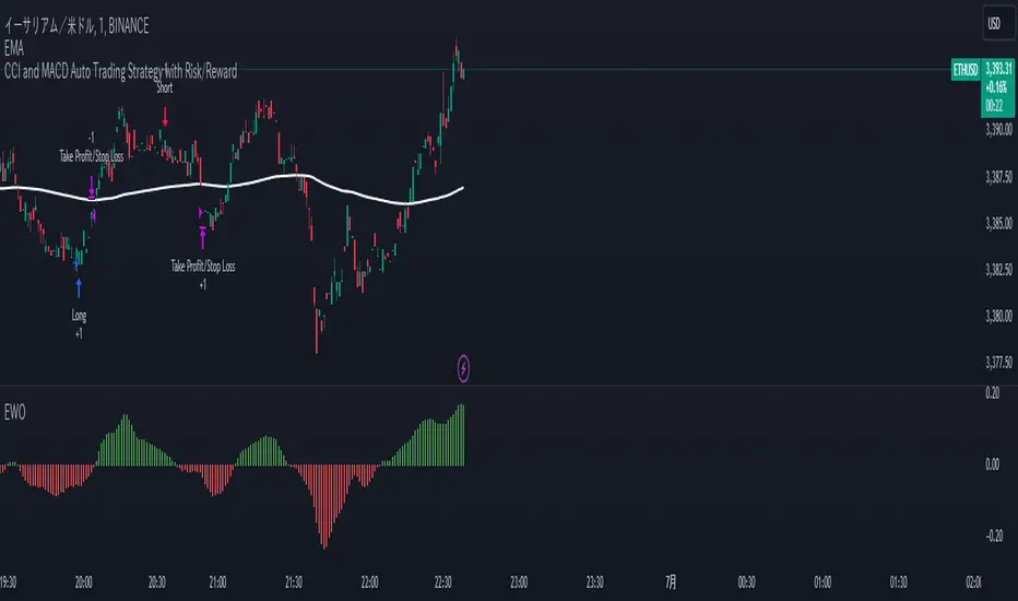
CCI and MACD Auto Trading Strategy with Risk/RewardOverview:
This strategy combines the Commodity Channel Index (CCI) and the Moving Average Convergence Divergence (MACD) indicators to automate trading decisions. It dynamically sets stop-loss and take-profit levels based on recent lows and highs, ensuring a risk/reward ratio of 1:1.5. This script aims to leverage trend and momentum signals while maintaining effective risk management.
Originality and Usefulness:
This script is not just a simple mashup of CCI and MACD indicators; it incorporates dynamic risk management by setting stop-loss and take-profit levels based on recent price action. This approach helps traders to:
・Identify potential trend reversals using the combination of CCI and MACD signals.
・Manage trades effectively by setting realistic stop-loss and take-profit levels based on recent market data.
・Maintain a balanced risk/reward ratio, which is essential for sustainable trading.
Indicators Used:
・CCI (Commodity Channel Index):
・Measures the deviation of the price from its average over a specified period, typically ranging from -100 to +100.
・Helps identify overbought and oversold conditions.
・MACD (Moving Average Convergence Divergence):
・Utilizes the difference between short-term and long-term moving averages to indicate trend strength and direction.
・Provides momentum signals that can be used for timing entries and exits.
How It Works:
Entry Conditions:
Long Entry:
・The MACD histogram is above zero.
・The CCI crosses above the -100 line.
Short Entry:
・The MACD histogram is below zero.
・The CCI crosses below the +100 line.
Exit Conditions:
Long Positions:
・The stop-loss is set at the recent low.
・The take-profit is set at 1.5 times the distance between the entry price and the stop-loss.
Short Positions:
・The stop-loss is set at the recent high.
・The take-profit is set at 1.5 times the distance between the entry price and the stop-loss.
Risk Management:
・The script dynamically adjusts stop-loss and take-profit levels based on recent market data, ensuring that the risk/reward ratio is maintained at 1:1.5.
・This approach helps in managing the risk effectively while aiming for consistent profits.
Strategy Properties:
・Account Size: Configured for a realistic account size suitable for the average trader.
・Commission and Slippage: Includes settings for realistic commission and slippage to reflect real market conditions.
・Risk per Trade: Designed to risk no more than 5-10% of equity per trade, aligning with sustainable trading practices.
・Backtesting Results: Configured to generate a sufficient sample size (ideally more than 100 trades) for reliable backtesting results.
Revised Backtesting Settings
Ensure that your backtesting settings are realistic:
・Account Size: Set a realistic initial capital suitable for the average trader.
・Commission and Slippage: Include realistic commission fees and slippage.
・Risk Management: Ensure that each trade risks no more than 5-10% of the account equity.
・Sufficient Sample Size: Choose a dataset that will generate more than 100 trades to provide a robust sample size.
ICT KillZones + Pivot Points [TradingFinder] Support/Resistance 🟣 Introduction
Pivot Points are critical levels on a price chart where trading activity is notably high. These points are derived from the prior day's price data and serve as key reference markers for traders' decision-making processes.
Types of Pivot Points :
Floor
Woodie
Camarilla
Fibonacci
🔵 Floor Pivot Points
Widely utilized in technical analysis, floor pivot points are essential in identifying support and resistance levels. The central pivot point (PP) acts as the primary level, suggesting the trend's likely direction.
The additional resistance levels (R1, R2, R3) and support levels (S1, S2, S3) offer further insight into potential trend reversals or continuations.
🔵 Camarilla Pivot Points
Featuring eight distinct levels, Camarilla pivot points closely correspond with support and resistance, making them highly effective for setting stop-loss orders and profit targets.
🔵 Woodie Pivot Points
Similar to floor pivot points, Woodie pivot points differ by placing greater emphasis on the closing price, often resulting in different pivot levels compared to the floor method.
🔵 Fibonacci Pivot Points
Fibonacci pivot points combine the standard floor pivot points with Fibonacci retracement levels applied to the previous trading period's range. Common retracement levels used are 38.2%, 61.8%, and 100%.
🟣 Sessions
Financial markets are divided into specific time segments, known as sessions, each with unique characteristics and activity levels. These sessions are active at different times throughout the day.
The primary sessions in financial markets include :
Asian Session
European Session
New York Session
The timing of these major sessions in UTC is as follows :
Asian Session: 23:00 to 06:00
European Session: 07:00 to 14:25
New York Session: 14:30 to 22:55
🟣 Kill Zones
Kill zones are periods within a session marked by heightened trading activity. During these times, trading volume surges and price movements become more pronounced.
The timing of the major kill zones in UTC is :
Asian Kill Zone: 23:00 to 03:55
European Kill Zone: 07:00 to 09:55
New York Kill Zone: 14:30 to 16:55
Combining kill zones and pivot points in financial market analysis provides several advantages :
Enhanced Market Sentiment Analysis : Aligns key price levels with high-activity periods for a clearer market sentiment.
Improved Timing for Trade Entries and Exits : Helps better time trades based on when price movements are most likely.
Higher Probability of Successful Trades : Increases the accuracy of predicting market movements and placing profitable trades.
Strategic Stop-Loss and Profit Target Placement : Allows for precise risk management by strategically setting stop-loss and profit targets.
Versatility Across Different Time Frames : Effective in both short and long time frames, suitable for various trading strategies.
Enhanced Trend Identification and Confirmation : Confirms trends using both pivot levels and high-activity periods, ensuring stronger trend validation.
In essence, this integrated approach enhances decision-making, optimizes trading performance, and improves risk management.
🟣 How to Use
🔵 Two Approaches to Trading Pivot Points
There are two main strategies for trading pivot points: utilizing "pivot point breakouts" and "price reversals."
🔵 Pivot Point Breakout
When the price breaks through pivot lines, it signals a shift in market sentiment to the trader. In the case of an upward breakout, where the price crosses these pivot lines, a trader might enter a long position, placing their stop-loss just below the pivot point (P).
Conversely, if the price breaks downward, a short position can be initiated below the pivot point. When using the pivot point breakout strategy, the first and second support levels can serve as profit targets in an upward trend. In a downward trend, these roles are filled by the first and second resistance levels.
🔵 Price Reversal
An alternative method involves waiting for the price to reverse at the support and resistance levels. To implement this strategy, traders should take positions opposite to the prevailing trend as the price rebounds from the pivot point.
While this tool is commonly used in higher time frames, it tends to produce better results in shorter time frames, such as 1-hour, 30-minute, and 15-minute intervals.
Three Strategies for Trading the Kill Zone
There are three principal strategies for trading within the kill zone :
Kill Zone Hunt
Breakout and Pullback to Kill Zone
Trading in the Trend of the Kill Zone
🔵 Kill Zone Hunt
This strategy involves waiting until the kill zone concludes and its high and low lines are established. If the price reaches one of these lines within the same session and is strongly rejected, a trade can be executed.
🔵 Breakout and Pullback to Kill Zone
In this approach, once the kill zone ends and its high and low lines stabilize, a trade can be made if the price breaks one of these lines decisively within the same session and then pulls back to that level.
🔵 Trading in the Trend of the Kill Zone
Kill zones are characterized by high trading volumes and strong trends. Therefore, trades can be placed in the direction of the prevailing trend. For instance, if an upward trend dominates this area, a buy trade can be entered when the price reaches a demand order block.

Sniper Entry using RSI confirmationThis is a sniper entry indicator that provides Buy and Sell signals using other Indicators to give the best possible Entries (note: Entries will not be 100 percent accurate and analysis should be done to support an entry)
Moving Average Crossovers:
The indicator uses two moving averages: a short-term SMA (Simple Moving Average) and a long-term SMA.
When the short-term SMA crosses above the long-term SMA, it generates a buy signal (indicating potential upward momentum).
When the short-term SMA crosses below the long-term SMA, it generates a sell signal (indicating potential downward momentum).
RSI Confirmation:
The indicator incorporates RSI (Relative Strength Index) to confirm the buy and sell signals generated by the moving average crossovers.
RSI is used to gauge the overbought and oversold conditions of the market.
A buy signal is confirmed if RSI is below a specified overbought level, indicating potential buying opportunity.
A sell signal is confirmed if RSI is above a specified oversold level, indicating potential selling opportunity.
Dynamic Take Profit and Stop Loss:
The indicator calculates dynamic take profit and stop loss levels based on the Average True Range (ATR).
ATR is used to gauge market volatility, and the take profit and stop loss levels are adjusted accordingly.
This feature helps traders to manage their risk effectively by setting appropriate profit targets and stop loss levels.
Combining the information provided by these, the indicator will provide an entry point with a provided take profit and stop loss. The indicator can be applied to different asset classes. Risk management must be applied when using this indicator as it is not 100% guaranteed to be profitable.
Goodluck!
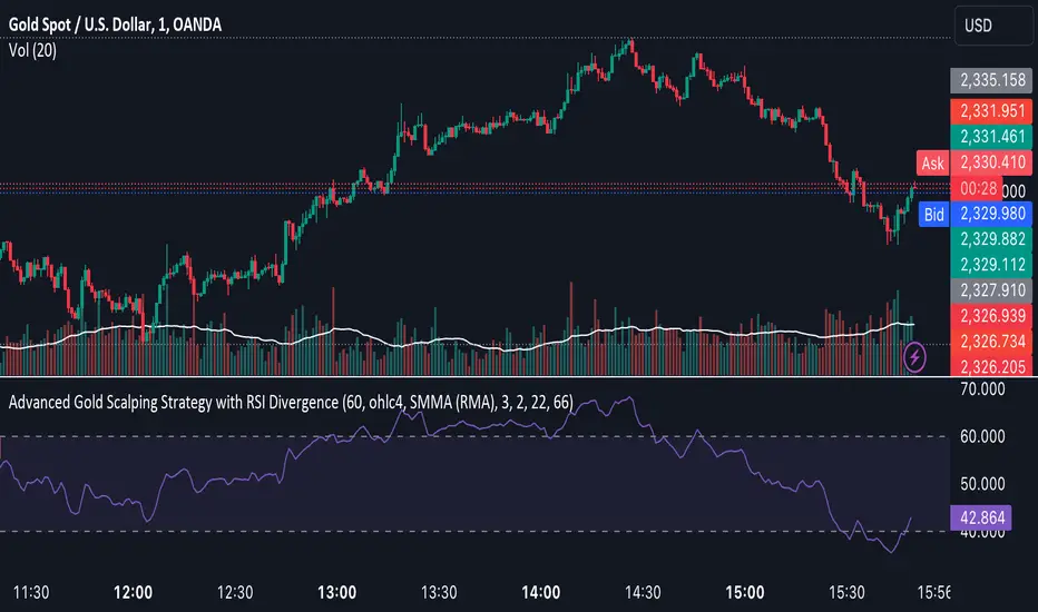
Advanced Gold Scalping Strategy with RSI Divergence# Advanced Gold Scalping Strategy with RSI Divergence
## Overview
This Pine Script implements an advanced scalping strategy for gold (XAUUSD) trading, primarily designed for the 1-minute timeframe. The strategy utilizes the Relative Strength Index (RSI) indicator along with its moving average to identify potential trade setups based on divergences between price action and RSI movements.
## Key Components
### 1. RSI Calculation
- Uses a customizable RSI length (default: 60)
- Allows selection of the source for RSI calculation (default: close price)
### 2. Moving Average of RSI
- Supports multiple MA types: SMA, EMA, SMMA (RMA), WMA, VWMA, and Bollinger Bands
- Customizable MA length (default: 3)
- Option to display Bollinger Bands with adjustable standard deviation multiplier
### 3. Divergence Detection
- Implements both bullish and bearish divergence identification
- Uses pivot high and pivot low points to detect divergences
- Allows for customization of lookback periods and range for divergence detection
### 4. Entry Conditions
- Long Entry: Bullish divergence when RSI is below 40
- Short Entry: Bearish divergence when RSI is above 60
### 5. Trade Management
- Stop Loss: Customizable, default set to 11 pips
- Take Profit: Customizable, default set to 33 pips
### 6. Visualization
- Plots RSI line and its moving average
- Displays horizontal lines at 30, 50, and 70 RSI levels
- Shows Bollinger Bands when selected
- Highlights divergences with "Bull" and "Bear" labels on the chart
## Input Parameters
- RSI Length: Adjusts the period for RSI calculation
- RSI Source: Selects the price source for RSI (close, open, high, low, hl2, hlc3, ohlc4)
- MA Type: Chooses the type of moving average applied to RSI
- MA Length: Sets the period for the moving average
- BB StdDev: Adjusts the standard deviation multiplier for Bollinger Bands
- Show Divergence: Toggles the display of divergence labels
- Stop Loss: Sets the stop loss distance in pips
- Take Profit: Sets the take profit distance in pips
## Strategy Logic
1. **RSI Calculation**:
- Computes RSI using the specified length and source
- Calculates the chosen type of moving average on the RSI
2. **Divergence Detection**:
- Identifies pivot points in both price and RSI
- Checks for higher lows in RSI with lower lows in price (bullish divergence)
- Checks for lower highs in RSI with higher highs in price (bearish divergence)
3. **Trade Entry**:
- Enters a long position when a bullish divergence is detected and RSI is below 40
- Enters a short position when a bearish divergence is detected and RSI is above 60
4. **Position Management**:
- Places a stop loss order at the entry price ± stop loss pips (depending on the direction)
- Sets a take profit order at the entry price ± take profit pips (depending on the direction)
5. **Visualization**:
- Plots the RSI and its moving average
- Draws horizontal lines for overbought/oversold levels
- Displays Bollinger Bands if selected
- Shows divergence labels on the chart for identified setups
## Usage Instructions
1. Apply the script to a 1-minute XAUUSD (Gold) chart in TradingView
2. Adjust the input parameters as needed:
- Increase RSI Length for less frequent but potentially more reliable signals
- Modify MA Type and Length to change the sensitivity of the RSI moving average
- Adjust Stop Loss and Take Profit levels based on current market volatility
3. Monitor the chart for Bull (long) and Bear (short) labels indicating potential trade setups
4. Use in conjunction with other analysis and risk management techniques
## Considerations
- This strategy is designed for short-term scalping and may not be suitable for all market conditions
- Always backtest and forward test the strategy before using it with real capital
- The effectiveness of divergence-based strategies can vary depending on market trends and volatility
- Consider using additional confirmation signals or filters to improve the strategy's performance
Remember to adapt the strategy parameters to your risk tolerance and trading style, and always practice proper risk management.
Sharpe and Sortino Ratios█ OVERVIEW
This indicator calculates the Sharpe and Sortino ratios using a chart symbol's periodic price returns, offering insights into the symbol's risk-adjusted performance. It features the option to calculate these ratios by comparing the periodic returns to a fixed annual rate of return or the returns from another selected symbol's context.
█ CONCEPTS
Returns, risk, and volatility
The return on an investment is the relative gain or loss over a period, often expressed as a percentage. Investment returns can originate from several sources, including capital gains, dividends, and interest income. Many investors seek the highest returns possible in the quest for profit. However, prudent investing and trading entails evaluating such returns against the associated risks (i.e., the uncertainty of returns and the potential for financial losses) for a clearer perspective on overall performance and sustainability.
The profitability of an investment typically comes at the cost of enduring market swings, noise, and general uncertainty. To navigate these turbulent waters, investors and portfolio managers often utilize volatility , a measure of the statistical dispersion of historical returns, as a foundational element in their risk assessments because it provides a tangible way to gauge the uncertainty in returns. High volatility suggests increased uncertainty and, consequently, higher risk, whereas low volatility suggests more stable returns with minimal fluctuations, implying lower risk. These concepts are integral components in several risk-adjusted performance metrics, including the Sharpe and Sortino ratios calculated by this indicator.
Risk-free rate
The risk-free rate represents the rate of return on a hypothetical investment carrying no risk of financial loss. This theoretical rate provides a benchmark for comparing the returns on a risky investment and evaluating whether its excess returns justify the risks. If an investment's returns are at or below the theoretical risk-free rate or the risk premium is below a desired amount, it may suggest that the returns do not compensate for the extra risk, which might be a call to reassess the investment.
Since the risk-free rate is a theoretical concept, investors often utilize proxies for the rate in practice, such as Treasury bills and other government bonds. Conventionally, analysts consider such instruments "risk-free" for a domestic holder, as they are a form of government obligation with a low perceived likelihood of default.
The average yield on short-term Treasury bills, influenced by economic conditions, monetary policies, and inflation expectations, has historically hovered around 2-3% over the long term. This range also aligns with central banks' inflation targets. As such, one may interpret a value within this range as a minimum proxy for the risk-free rate, as it may correspond to the minimum rate required to maintain purchasing power over time. This indicator uses a default value of 2% as the risk-free rate in its Sharpe and Sortino ratio calculations. Users can adjust this value from the "Risk-free rate of return" input in the "Settings/Inputs" tab.
Sharpe and Sortino ratios
The Sharpe and Sortino ratios are two of the most widely used metrics that offer insight into an investment's risk-adjusted performance . They provide a standardized framework to compare the effectiveness of investments relative to their perceived risks. These metrics can help investors determine whether the returns justify the risks taken to achieve them, promoting more informed investment decisions.
Both metrics measure risk-adjusted performance similarly. However, they have some differences in their formulas and their interpretation:
1. Sharpe ratio
The Sharpe ratio , developed by Nobel laureate William F. Sharpe, measures the performance of an investment compared to a theoretically risk-free asset, adjusted for the investment risk. The ratio uses the following formula:
Sharpe Ratio = (𝑅𝑎 − 𝑅𝑓) / 𝜎𝑎
Where:
• 𝑅𝑎 = Average return of the investment
• 𝑅𝑓 = Theoretical risk-free rate of return
• 𝜎𝑎 = Standard deviation of the investment's returns (volatility)
A higher Sharpe ratio indicates a more favorable risk-adjusted return, as it signifies that the investment produced higher excess returns per unit of increase in total perceived risk.
2. Sortino ratio
The Sortino ratio is a modified form of the Sharpe ratio that only considers downside volatility , i.e., the volatility of returns below the theoretical risk-free benchmark. Although it shares close similarities with the Sharpe ratio, it can produce very different values, especially when the returns do not have a symmetrical distribution, since it does not penalize upside and downside volatility equally. The ratio uses the following formula:
Sortino Ratio = (𝑅𝑎 − 𝑅𝑓) / 𝜎𝑑
Where:
• 𝑅𝑎 = Average return of the investment
• 𝑅𝑓 = Theoretical risk-free rate of return
• 𝜎𝑑 = Downside deviation (standard deviation of negative excess returns, or downside volatility)
The Sortino ratio offers an alternative perspective on an investment's return-generating efficiency since it does not consider upside volatility in its calculation. A higher Sortino ratio signifies that the investment produced higher excess returns per unit of increase in perceived downside risk.
The risk-free rate (𝑅𝑓) in the numerator of both ratio formulas acts as a baseline for comparing an investment's performance to a theoretical risk-free alternative. By subtracting the risk-free rate from the expected return (𝑅𝑎−𝑅𝑓), the numerator essentially represents the risk premium of the investment.
Comparison with another symbol
In addition to the conventional Sharpe and Sortino ratios, which compare an instrument's returns to a risk-free rate, this indicator can also compare returns to a user-specified benchmark symbol , allowing the calculation of Information ratios .
An Information ratio is a generalized form of the Sharpe ratio that compares an investment's returns to a risky benchmark , such as SPY, rather than a risk-free rate. It measures the investment's active return (the difference between its returns and the benchmark returns) relative to its tracking error (i.e., the volatility of the active return) using the following formula:
𝐼𝑅 = (𝑅𝑝 − 𝑅𝑏) / 𝑇𝐸
Where:
• 𝑅𝑝 = Average return on the portfolio or investment
• 𝑅𝑏 = Average return from the benchmark instrument
• 𝑇𝐸 = Tracking error (volatility of 𝑅𝑝 − 𝑅𝑏)
Comparing returns to a benchmark instrument rather than a theoretical risk-free rate offers unique insights into risk-adjusted performance. Higher Information ratios signify that the investment produced higher active returns per unit of increase in risk relative to the benchmark. Conventional choices for non-risk-free benchmarks include major composite indices like the S&P 500 and DJIA, as the resulting ratios can provide insight into the effectiveness of an investment relative to the broader market.
Users can enable this generalized calculation for both the Sharpe and Sortino ratios by selecting the "Benchmark symbol returns" option from the "Benchmark type" dropdown in the "Settings/Inputs" tab.
It's crucial to note that this indicator compares the charts symbol's rate of change (return) to the rate of change in the benchmark symbol. Consequently, not all symbols available on TradingView are suitable for use with these ratios due to the nature of what their values represent. For instance, using a bond as a benchmark will produce distorted results since each bar's values represent yields rather than prices, meaning it compares the rate of change in the yield. To maintain consistency and relevance in the calculated ratios, ensure the values from the compared symbols strictly represent price information.
█ FEATURES
This indicator provides traders with two widely used metrics for assessing risk-adjusted performance, generalized to allow users to compare the chart symbol's price returns to a fixed risk-free rate or the returns from another risky symbol. Below are the key features of this indicator:
Timeframe selection
The "Returns timeframe" input determines the timeframe of the calculated price returns. Users can select any value greater than or equal to the chart's timeframe. The default timeframe is "1M".
Periodic returns tracking
This indicator compounds and collects requested price returns from the selected timeframe over monthly or daily periods, similar to how the Broker Emulator works when calculating strategy performance metrics on trade data. It employs the following logic:
• Track returns over monthly periods if the chart's data spans at least two months.
• Track returns over daily periods if the chart's data spans at least two days but not two months.
• Do not track or collect returns if the data spans less than two days, as the amount of data is insufficient for meaningful ratio calculations.
The indicator uses the returns collected from up to a specified number of periods to calculate the Sharpe and Sortino ratios, depending on the available historical data. It also uses these periodic returns to calculate the average returns it displays in the Data Window.
Users can control the maximum number of periods the indicator analyzes with the "Max no. of periods used" input in the "Settings/Inputs" tab. The default value is 60 periods.
Benchmark specification
The "Benchmark return type" input specifies the benchmark type the indicator compares to the chart symbol's returns in the ratio calculations. It features the following two options:
• "Risk-free rate of return (%)": Compares the price returns to a user-specified annual rate of return representing a theoretical risk-free rate (e.g., 2%).
• "Benchmark symbol return": Compares the price returns to a selected benchmark symbol (e.g., "AMEX:SPY) to calculate Information ratios.
When comparing a chart symbol's returns to a specified benchmark symbol, this indicator aligns the times of data points from the benchmark with the times of data points from the chart's symbol to facilitate a fair comparison between symbols with different active sessions.
Visualization and display
• The indicator displays the periodic returns requested from the specified "Returns timeframe" in a separate pane. The plot includes dynamic colors to signify positive and negative returns.
• When the "Returns timeframe" value represents a higher timeframe, the indicator displays background highlights on the main chart pane to signify when a new value is available and whether the return is positive or negative.
• When the specified benchmark return type is a benchmark symbol, the indicator displays the requested symbol's returns in the separate pane as a gray line for visual comparison.
• Within the separate pane, the indicator displays a single-cell table that shows the base period it uses for periodic returns, the number of periods it uses in the calculation, the timeframe of the requested data, and the calculated Sharpe and Sortino ratios.
• The Data Window displays the chart symbol and benchmark returns, their periodic averages, and the Sharpe and Sortino ratios.
█ FOR Pine Script™ CODERS
• This script utilizes the functions from our RiskMetrics library to determine the size of the periods, calculate and collect periodic returns, and compute the Sharpe and Sortino ratios.
• The `getAlignedPrices()` function in this script requests price data for the chart's symbol and a benchmark symbol with consistent time alignment by utilizing spread symbols , which helps facilitate a fair comparison between different symbol types. Retrieving prices from spreads avoids potential information loss and data misalignment that can otherwise occur when using separate requests from each symbol's context when those symbols have different sessions or data times.
• For consistency, the `getAlignedPrices()` function includes extended hours and dividend adjustment modifiers in its data requests. Additionally, it includes other settings inherited from the chart's context, such as "settlement-as-close" preferences for fair comparison between futures instruments.
• This script uses the `changePercent()` function from our ta library to calculate the percentage changes of the requested data.
• The newly released `force_overlay` parameter in display-related functions allows indicators to display visuals on the main chart and a separate pane simultaneously. We use the parameter in this script's bgcolor() call to display background highlights on the main chart.
Look first. Then leap.

Pivot PointsPivot points are technical indicators used in financial markets (such as stocks, forex, or commodities) to identify potential turning points in price movement. They provide reference levels based on the previous day’s price action.
How to use the Pivot Points indicator
Traders use pivot points to identify significant price levels where the market may reverse or consolidate.
PP, S1, and R1 are considered primary levels, while S2 and R2 are secondary levels.
R3, R4, R5, S3, S4 and S5 are considered more extreme levels and we normally don't see price action trade near these levels on a typical day. This indicator calculates those extreme levels to help on days with extreme price action.
Pivot points can be calculated for different timeframes (daily, weekly, monthly, quarterly, 6-months and yearly).
Pivot points calculated using the daily timeframe is a popular chose among day traders traders who trade intraday timeframes.
Trading Strategies
Bounce Strategy:
Buy near support (S1 or S2) if the price bounces off these levels.
Sell near resistance (R1 or R2) if the price reverses from these levels.
Breakout Strategy:
If the price breaks above R1, consider a long position.
If the price breaks below S1, consider a short position.
Profit targets:
If in a long trade and price hits R1, you take some profit.
If in a short trade and price hits S1, you take some profit.
Combine pivot points with other technical indicators (e.g., moving averages, candlestick patterns) for confirmation. Remember that pivot points are just one tool among many, and their effectiveness varies across different markets and timeframes. Always practice risk management and consider the overall market context when using pivot points in your trading decisions.

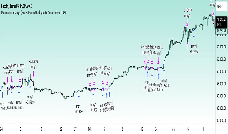
Momentum Alligator 4h Bitcoin StrategyOverview
The Momentum Alligator 4h Bitcoin Strategy is a trend-following trading system that operates on dual time frames. It utilizes the 1D Williams Alligator indicator to identify the prevailing major price trend and seeks trading opportunities on the 4-hour (4h) time frame when the momentum is turning up. The strategy is designed to close trades if the trend fails to develop or holding position if price continues increasing without any significant correction. Note that this strategy is specifically tailored for the 4-hour time frame.
Unique Features
2-layers market noise filtering system: Trades are only initiated in the direction of the 1D trend, determined by the Williams Alligator indicator. This higher time frame confirmation filters out minor trade signals, focusing on more substantial opportunities. At the same time, strategy has additional filter on 4h time frame with Awesome Oscillator which is showing the current price momentum.
Flexible Risk Management: The strategy exclusively opens long positions, resulting in fewer trades during bear markets. It incorporates a dynamic stop-loss mechanism, which can either follow the jaw line of the 4h Alligator or a user-defined fixed stop-loss. This flexibility helps manage risk and avoid non-trending markets.
Methodology
The strategy initiates a long position when the d-line of Stochastic RSI crosses up it's k-line. It means that there is a high probability that price momentum reversed from down to up. To avoid overtrading in potentially choppy markets, it skips the next two trades following a winning trade, anticipating sideways movement after a significant price surge.
This strategy has two layers trades filtering system: 4h and 1D time frames. The first one is awesome oscillator. It shall be increasing and value has to be higher than it's 5-period SMA. This is an additional confirmation that long trade is opened in the direction of the current momentum. As it was mentioned above, all entry signals are validated against the 1D Williams Alligator indicator. A trade is only opened if the price is above all three lines of the 1D Alligator, ensuring alignment with the major trend.
A trade is closed if the price hits the 4h jaw line of the Alligator or reaches the user-defined stop-loss level.
Risk Management
The strategy employs a combined approach to risk management:
It allows positions to ride the trend as long as the price continues to move favorably, aiming to capture significant price movements. It features a user-defined stop-loss parameter to mitigate risks based on individual risk tolerance. By default, this stop-loss is set to a 2% drop from the entry point, but it can be adjusted according to the trader's preferences.
Justification of Methodology
This strategy leverages Stochastic RSI on 4h time frame to open long trade when momentum started reversing to the upside. On the one hand, Stochastic RSI is one of the most sensitive indicator, which allows to react fast on the potential trend reversal. On the other hand, this indicator can be too sensitive and provide a lot of false trend changing signals. To eliminate this weakness we use two-layers trades filtering system.
The first layer is the 4h Awesome oscillator. This is less sensitive momentum indicator. Usually it starts increasing when price has already passed significant distance from the actual reversal point. The strategy opens long trade only is Awesome oscillator is increasing and above it's 5-period SMA. This approach increases the probability to filter the false signals during the choppy market or if the reversal is false.
The second layer filter is the Williams Alligator indicator on 1D time frame. The 1D Alligator serves as a filter for identifying the primary trend and increases probability to avoid the trades with low potential because trading against major trend usually is more risky. It's much better to catch the trend continuation than local bounce.
Last but not least feature of this strategy is close trades condition. It uses the flexible approach. First of all, user can set up the fixed stop-loss according to his own risk-tolerance, by default this value is 2% of price movement. It restricts the potential loss at the moment when trade has just been opened. Moreover strategy utilizes the 4h Williams Alligator's jaw line to exit the trade. If price fell below it trade is closed. This approach helps to not keep open trade if trend is not developing and hold it if price continues going up.
Backtest Results:
Operating window: Date range of backtests is 2021.01.01 - 2024.05.01. It is chosen to let the strategy to close all opened positions.
Commission and Slippage: Includes a standard Binance commission of 0.1% and accounts for possible slippage over 5 ticks.
Initial capital: 10000 USDT
Percent of capital used in every trade: 50%
Maximum Single Position Loss: -3.04%
Maximum Single Profit: +29.67%
Net Profit: +6228.01 USDT (+62.28%)
Total Trades: 118 (24.58% win rate)
Profit Factor: 1.71
Maximum Accumulated Loss: 1527.69 USDT (-11.52%)
Average Profit per Trade: 52.78 USDT (+0.89%)
Average Trade Duration: 60 hours
These results are obtained with realistic parameters representing trading conditions observed at major exchanges such as Binance and with realistic trading portfolio usage parameters.
How to Use:
Add the script to favorites for easy access.
Apply to the 4h timeframe desired chart (optimal performance observed on the BTC/USDT).
Configure settings using the dropdown choice list in the built-in menu.
Set up alerts to automate strategy positions through web hook with the text: {{strategy.order.alert_message}}
Disclaimer:
Educational and informational tool reflecting Skyrex commitment to informed trading. Past performance does not guarantee future results. Test strategies in a simulated environment before live implementation
[InvestorUnknown] Performance MetricsOverview
The Performance Metrics indicator is a tool designed to help traders and investors understand and utilize key performance metrics in their strategies. This indicator is inspired by the Rolling Risk-Adjusted Performance Ratios created by @EliCobra, but it offers enhanced usability and additional features to provide a more user-friendly code for understanding the calculations.
Features
Rolling Lookback:
Dynamic Lookback Calculation: The indicator automatically calculates the number of bars from the start of the asset's price history, up to a maximum of 5000 bars due to TradingView platform restrictions.
Adjustable Lookback Period: Users can manually set a lookback period or choose to use the rolling lookback feature for dynamic calculations.
RollingLookback() =>
x = bar_index + 1
y = x > 4999 ? 5000 : x > 1 ? (x - 1) : x
y
Trend Analysis
The Trend Analysis section in this indicator helps traders identify the direction of the market trend based on the balance of positive and negative returns over time. This is achieved by calculating the sums of positive and negative returns and optionally smoothing these values to provide a clearer trend signal.
Configuration: Enable smoothing if you want to reduce noise in the trend analysis. Choose between EMA and SMA for smoothing. Set the length for smoothing according to your preference for sensitivity (shorter lengths are more sensitive to changes, longer lengths provide smoother signals).
Interpretation:
- A positive trend difference (filled with green) indicates a bullish trend, suggesting more positive returns.
- A negative trend difference (filled with red) indicates a bearish trend, suggesting more negative returns.
- Colored bars provide a quick visual cue on the trend direction, helping to make timely trading decisions.
// The Trend Analysis section calculates and optionally smooths the sums of positive and negative returns.
// This helps identify the trend direction based on the balance of positive and negative returns over time.
Ps = Smooth ? Smooth_type == "EMA" ? ta.ema(pos_sum, Smooth_len) : ta.sma(pos_sum, Smooth_len) : pos_sum
Ns = Smooth ? Smooth_type == "EMA" ? ta.ema(neg_sum, Smooth_len) : ta.sma(neg_sum, Smooth_len) : neg_sum
// Calculate the difference between smoothed positive and negative sums
dif = Ps + Ns
Performance Metrics Table
Visual Table Display: Option to display a table on the chart with calculated performance metrics. This table includes comprehensive metrics like Mean Return, Positive and Negative Mean Return, Standard Deviation, Sharpe Ratio, Sortino Ratio, and Omega Ratio.
Performance Metrics Calculated
Mean Return:
Description: The average return over the lookback period.
Purpose: Helps in understanding the overall performance of the asset by providing a simple average of returns.
Positive Mean Return:
Description: The average of all positive returns over the lookback period.
Purpose: Highlights the average gain during profitable periods, giving insight into the asset's potential upside.
Negative Mean Return:
Description: The average of all negative returns over the lookback period.
Purpose: Focuses on the average loss during unprofitable periods, helping to assess the downside risk.
Standard Deviation (STDEV):
Description: A measure of volatility that calculates the dispersion of returns from the mean.
Purpose: Indicates the risk associated with the asset. Higher standard deviation means higher volatility and risk.
Sharpe Ratio:
Description: A risk-adjusted return metric that divides the mean return by the standard deviation of returns. It can be annualized if selected.
Purpose: Provides a standardized way to compare the performance of different assets by considering both return and risk. A higher Sharpe Ratio indicates better risk-adjusted performance.
sharpe_ratio = mean_all / stddev_all * (Annualize ? math.sqrt(Lookback) : 1)
Sortino Ratio:
Description: Similar to the Sharpe Ratio but focuses only on downside volatility. It divides the mean return by the standard deviation of negative returns. It can be annualized if selected.
Purpose: Offers a better assessment of downside risk by ignoring upside volatility. A higher Sortino Ratio indicates a higher return per unit of downside risk.
sortino_ratio = mean_all / stddev_neg * (Annualize ? math.sqrt(Lookback) : 1)
Omega Ratio:
Description: The ratio of the probability-weighted average of positive returns to the probability-weighted average of negative returns.
Purpose: Measures the overall likelihood of positive returns compared to negative returns. An Omega Ratio greater than 1 indicates more frequent and/or larger positive returns compared to negative returns.
omega_ratio = (prob_pos * mean_pos) / (prob_neg * -mean_neg)
By calculating and displaying these metrics, the indicator provides a comprehensive view of the asset's performance, enabling traders and investors to make informed decisions based on both returns and risk-adjusted metrics.
Use Cases:
Performance Evaluation: Assesses an asset's performance by analyzing both returns and risk factors, giving a clear picture of profitability and volatility.
Risk Comparison: Compares the risk-adjusted returns of different assets or portfolios, aiding in identifying investments with superior risk-reward trade-offs.
Risk Management: Helps manage risk exposure by evaluating downside risks and overall volatility, enabling more informed and strategic investment decisions.

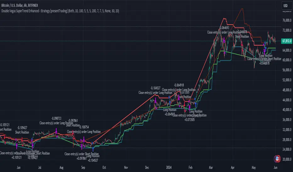
Double Vegas SuperTrend Enhanced - Strategy [presentTrading]
█ Introduction and How It Is Different
The "Double Vegas SuperTrend Enhanced" strategy is a sophisticated trading system that combines two Vegas SuperTrend Enhanced. Very Powerful!
Let's celebrate the joy of Children's Day on June 1st! Enjoyyy!
BTCUSD LS performance
The strategy aims to pinpoint market trends with greater accuracy and generate trades that align with the overall market direction.
This approach differentiates itself by integrating volatility adjustments and leveraging the Vegas Channel's width to refine the SuperTrend calculations, resulting in a dynamic and responsive trading system.
Additionally, the strategy incorporates customizable take-profit and stop-loss levels, providing traders with a robust framework for risk management.
-> check Vegas SuperTrend Enhanced - Strategy
█ Strategy, How It Works: Detailed Explanation
🔶 Vegas Channel and SuperTrend Calculations
The strategy initiates by calculating the Vegas Channel, which is derived from a simple moving average (SMA) and the standard deviation (STD) of the closing prices over a specified window length. This channel helps in measuring market volatility and forms the basis for adjusting the SuperTrend indicator.
Vegas Channel Calculation:
- vegasMovingAverage = SMA(close, vegasWindow)
- vegasChannelStdDev = STD(close, vegasWindow)
- vegasChannelUpper = vegasMovingAverage + vegasChannelStdDev
- vegasChannelLower = vegasMovingAverage - vegasChannelStdDev
SuperTrend Multiplier Adjustment:
- channelVolatilityWidth = vegasChannelUpper - vegasChannelLower
- adjustedMultiplier = superTrendMultiplierBase + volatilityAdjustmentFactor * (channelVolatilityWidth / vegasMovingAverage)
The adjusted multiplier enhances the SuperTrend's sensitivity to market volatility, making it more adaptable to changing market conditions.
BTCUSD Local picture.
🔶 Average True Range (ATR) and SuperTrend Values
The ATR is computed over a specified period to measure market volatility. Using the ATR and the adjusted multiplier, the SuperTrend upper and lower levels are determined.
ATR Calculation:
- averageTrueRange = ATR(atrPeriod)
**SuperTrend Calculation:**
- superTrendUpper = hlc3 - (adjustedMultiplier * averageTrueRange)
- superTrendLower = hlc3 + (adjustedMultiplier * averageTrueRange)
The SuperTrend levels are continuously updated based on the previous values and the current market trend direction. The market trend is determined by comparing the closing prices with the SuperTrend levels.
Trend Direction:
- If close > superTrendLowerPrev, then marketTrend = 1 (bullish)
- If close < superTrendUpperPrev, then marketTrend = -1 (bearish)
🔶 Trade Entry and Exit Conditions
The strategy generates trade signals based on the alignment of both SuperTrends. Trades are executed only when both SuperTrends indicate the same market direction.
Entry Conditions:
- Long Position: Both SuperTrends must signal a bullish trend.
- Short Position: Both SuperTrends must signal a bearish trend.
Exit Conditions:
- Positions are exited if either SuperTrend reverses its trend direction.
- Additional conditions include holding periods and configurable take-profit and stop-loss levels.
█ Trade Direction
The strategy allows traders to specify the desired trade direction through a customizable input setting. Options include:
- Long: Only enter long positions.
- Short: Only enter short positions.
- Both: Enter both long and short positions based on the market conditions.
█ Usage
To utilize the "Double Vegas SuperTrend Enhanced" strategy, traders need to configure the input settings according to their trading preferences and market conditions. The strategy includes parameters for ATR periods, Vegas Channel window lengths, SuperTrend multipliers, volatility adjustment factors, and risk management settings such as hold days, take-profit, and stop-loss percentages.
█ Default Settings
The strategy comes with default settings that can be adjusted to fit individual trading styles:
- trade Direction: Both (allows trading in both long and short directions for maximum flexibility).
- ATR Periods: 10 for SuperTrend 1 and 5 for SuperTrend 2 (shorter ATR period results in more sensitivity to recent price movements).
- Vegas Window Lengths: 100 for SuperTrend 1 and 200 for SuperTrend 2 (longer window length results in smoother moving averages and less sensitivity to short-term volatility).
- SuperTrend Multipliers: 5 for SuperTrend 1 and 7 for SuperTrend 2 (higher multipliers lead to wider SuperTrend channels, reducing the frequency of trades).
- Volatility Adjustment Factors: 5 for SuperTrend 1 and 7 for SuperTrend 2 (higher adjustment factors increase the responsiveness to changes in market volatility).
- Hold Days: 5 (defines the minimum duration a position is held, ensuring trades are not exited prematurely).
- Take Profit: 30% (sets the target profit level to lock in gains).
- Stop Loss: 20% (sets the maximum acceptable loss level to mitigate risk).
Entry Fragger - Strategy
For basic instructions please visit my other script "Entry Fragger".
The Signal Logic is explained there.
v1.4:
- Added advanced backtesting with fully customizable entries.
- Fully automated Buy Signals (profitable).
- Adjustable timeframes for signal logic. (requested)
Every setting affects the accuracy and profitability greatly now, based on settings applied.
The strategy performs best on high timeframes with larger capital and no leverage.
Useless for Forex, but absolutely smashes stocks and crypto on mid to high timeframes.
Please read through my other scripts description.
Set values as preferred and try your assets.
It does NOT work on low timeframes and forex!
Hint: BTC 4H, Custom Timeframe 1h, Moon Mode and Show Sell Signals enabled, R2R: 2.

Trade Exit Calculator [MarketSignalsPro]█ OVERVIEW
This Pine Script calculates a Stop Loss and Take Profit order suggestion based on the Average True Range (ATR). This provides a market generated visual reference for the user to better gauge risk and profit potential for their trades. This is not a trade signal system, it is a tool best used in conjunction with an existing system.
█ FEATURES
Inputs:
stopLossMultiplier and takeProfitMultiplier : These are input parameters that allow the user to adjust the multiplier for calculating stop loss and take profit levels.
longIndicator : This input parameter determines whether the script is calculating levels for a long setup (buy) or a short setup (sell).
Variable Initialization:
Various variables are initialized to manage labels, lines, and calculated stop loss and take profit levels.
ATR (Average True Range) is calculated using a period of 14.
Calculation of Stop Loss and Take Profit:
Depending on the value of longIndicator stop loss and take profit levels are not calculated the same way.
For long setups, stop loss is calculated below the closing price and take profit above, while for short setups, it's the opposite.
The calculation involves multiplying the ATR value by the user-defined multipliers and adding or subtracting from the closing price accordingly.
Plotting Lines:
Lines representing the calculated stop loss, take profit, and entry price are plotted on the chart.
Displaying Labels:
Labels displaying the calculated stop loss, take profit, and entry price are shown on the chart alongside the respective lines.
Updating and Deleting Objects:
Existing lines and labels are updated or deleted to ensure only the most recent levels are displayed on the chart.
Final Output:
The script outputs visual representations of stop loss, take profit, and entry price levels on the chart, providing traders with guidance for risk management and profit-taking strategies based on the volatility of the market.
█ CONCLUSION
In summary, this Pine Script enhances trading strategies by calculating and illustrating stop loss and take profit levels based on the Average True Range indicator, offering traders a structured way to manage risk and profit potential.
█ THANKS
Special thanks to Cryptosnagger for taking the time to build this Pine Script and share it freely with the community.

Multi-Timeframe Trend Following with 200 EMA Filter - Longs OnlyOverview
This strategy is designed to trade long positions based on multiple timeframe Exponential Moving Averages (EMAs) and a 200 EMA filter. The strategy ensures that trades are only entered in strong uptrends and aims to capitalize on sustained upward movements while minimizing risk with a defined stop-loss and take-profit mechanism.
Key Components
Initial Capital and Position Sizing
Initial Capital: $1000.
Lot Size: 1 unit per trade.
Inputs
Fast EMA Length (fast_length): The period for the fast EMA.
Slow EMA Length (slow_length): The period for the slow EMA.
200 EMA Length (filter_length_200): Set to 200 periods for the primary trend filter.
Stop Loss Percentage (stop_loss_perc): Set to 1% of the entry price.
Take Profit Percentage (take_profit_perc): Set to 3% of the entry price.
Timeframes and EMAs
EMAs are calculated for the following timeframes using the request.security function:
5-minute: Short-term trend detection.
15-minute: Intermediate-term trend detection.
30-minute: Long-term trend detection.
The strategy also calculates a 200-period EMA on the 5-minute timeframe to serve as a primary trend filter.
Trend Calculation
The strategy determines the trend for each timeframe by comparing the fast and slow EMAs:
If the fast EMA is above the slow EMA, the trend is considered positive (1).
If the fast EMA is below the slow EMA, the trend is considered negative (-1).
Combined Trend Signal
The combined trend signal is derived by summing the individual trends from the 5-minute, 15-minute, and 30-minute timeframes.
A combined trend value of 3 indicates a strong uptrend across all timeframes.
Any combined trend value less than 3 indicates a weakening or negative trend.
Entry and Exit Conditions
Entry Condition:
A long position is entered if:
The combined trend signal is 3 (indicating a strong uptrend across all timeframes).
The current close price is above the 200 EMA on the 5-minute timeframe.
Exit Condition:
The long position is exited if:
The combined trend signal is less than 3 (indicating a weakening trend).
The current close price falls below the 200 EMA on the 5-minute timeframe.
Stop Loss and Take Profit
Stop Loss: Set at 1% below the entry price.
Take Profit: Set at 3% above the entry price.
These levels are automatically set when entering a trade using the strategy.entry function with stop and limit parameters.
Plotting
The strategy plots the fast and slow EMAs for the 5-minute timeframe and the 200 EMA for visual reference on the chart:
Fast EMA (5-min): Plotted in blue.
Slow EMA (5-min): Plotted in red.
200 EMA (5-min): Plotted in green.