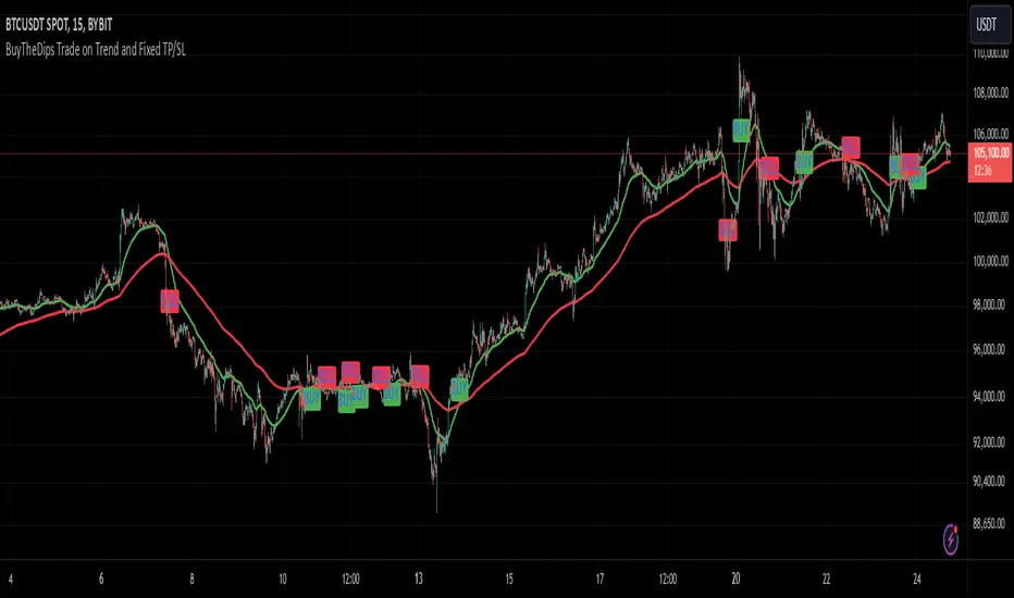
BuyTheDips Trade on Trend and Fixed TP/SL
This strategy is designed to trade in the direction of the trend using exponential moving average (EMA) crossovers as signals while employing fixed percentages for take profit (TP) and stop loss (SL) to manage risk and reward. It is suitable for both scalping and swing trading on any timeframe, with its default settings optimized for short-term price movements.
How It Works
EMA Crossovers:
The strategy uses two EMAs: a fast EMA (shorter period) and a slow EMA (longer period).
A buy signal is triggered when the fast EMA crosses above the slow EMA, indicating a potential bullish trend.
A sell signal is triggered when the fast EMA crosses below the slow EMA, signaling a bearish trend.
Trend Filtering:
To improve signal reliability, the strategy only takes trades in the direction of the overall trend:
Long trades are executed only when the fast EMA is above the slow EMA (bullish trend).
Short trades are executed only when the fast EMA is below the slow EMA (bearish trend).
This filtering ensures trades are aligned with the prevailing market direction, reducing false signals.
Risk Management (Fixed TP/SL):
The strategy uses fixed percentages for take profit and stop loss:
Take Profit: A percentage above the entry price for long trades (or below for short trades).
Stop Loss: A percentage below the entry price for long trades (or above for short trades).
These percentages can be customized to balance risk and reward according to your trading style.
For example:
If the take profit is set to 2% and the stop loss to 1%, the strategy operates with a 2:1 risk-reward ratio. BINANCE:BTCUSDT
Cerca negli script per "stop loss"
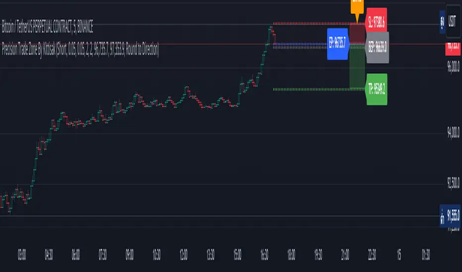
Precision Trade Zone By KittisakThis indicator is designed for Money Management calculations, helping to facilitate risk management in trading, determining suitable leverage based on acceptable risk, and adjusting the Stop Loss level to align with the calculated leverage.
Abbreviation Descriptions
LR : Suitable Leverage.
EP : Entry Price.
BEP : Break-Even Point (a point where you can move your Stop Loss to prevent losses once the price reaches a certain level).
SL : Stop Loss (a recalculated Stop Loss level to match the leverage. You should use this as the Stop Loss price instead of the initial level you set).
TP : Take Profit (a point where you take profit based on the defined risk-reward ratio).
Note
When first activating the indicator, an error may occur, and no output will be displayed. This happens because you must first specify the Entry Price and Stop Loss in the indicator settings.
How Much Leverage Should You Use?
It may seem like a simple question but is difficult to answer.
Method for Calculating Suitable Leverage
Use the formula:
Leverage = Acceptable Loss / (Distance between Entry Price and Stop Loss + (Buy Fee + Sell Fee))
Calculating the Correct Stop Loss Point
(Stop Loss levels will be slightly adjusted or extended)
For Long Positions :
New Stop Loss = Entry Price * (1 - Acceptable Loss / (Calculated Leverage * 100))
For Short Positions :
New Stop Loss = Entry Price * (1 + Acceptable Loss / (Calculated Leverage * 100))
Calculating the Correct Take Profit Point
(Take Profit levels will be slightly adjusted or extended)
For Long Positions :
Take Profit = Entry Price * (1 + (Acceptable Loss / (Calculated Leverage * 100) * RR) + ((Buy Fee + Sell Fee) / 100))
For Short Positions :
Take Profit = Entry Price * (1 - (Acceptable Loss / (Calculated Leverage * 100) * RR) + ((Buy Fee + Sell Fee) / 100))
Benefits of This Calculation
1. Accurate Risk Assessment
The calculated leverage accounts for trading fees. For example, if you aim for a 2% loss, this method ensures the actual loss is exactly 2%, not more (e.g., 2% plus fees).
2. Eliminates Guesswork
Randomly setting leverage can lead to risks because the Stop Loss level may not align with your position. This calculation ensures that the leverage aligns precisely with your desired Stop Loss level.
3. Realistic Profit Targets
For example, with a 2% acceptable loss and a 1:2 RR, you expect a 4% profit. However, without this calculation, fees may reduce your profit below 4%. This method includes fees, ensuring your profit matches the intended target.
Caution
This indicator does not account for slippage or requotes. Use it with caution and allow a buffer for slippage in your calculations.
Indicator นี้มีไว้สำหรับคำนวณ Money Management ซึ่งจะช่วยอำนวยความสะดวกในการจัดการความเสี่ยงในการเทรด การคำนวณ Leverage ที่เหมาะสมกับความเสี่ยงที่คุณยอมรับได้ และจัดการจุด Stop Loss ให้เหมาะสมกับ Leverage นั้น
คำอธิบายเกี่ยวกับคำย่อ
LR หมายถึง Leverage ที่เหมาะสม
EP หมายถึง Entry Price หรือราคาเข้าซื้อ
BEP หมายถึง Break-Even Point หรือจุดคุ้มทุน (คุณสามารถย้าย Stop Loss มาที่จุดนี้เมื่อราคาไปถึงจุดหนึ่งเพื่อป้องกันการขาดทุนได้)
SL หมายถึง Stop Loss (ซึ่งเป็น Stop Loss ที่คำนวณใหม่เพื่อให้ตำแหน่งเหมาะสมกับ Leverage ที่คำนวณได้ คุณควรใช้จุดนี้เพื่อเป็นราคา Stop Loss แทนจุด Stop Loss ที่คุณกำหนดไว้ในตอนแรก)
TP หมายถึง Take Profit (เป็นจุดที่คุณจะขายทำกำไรตาม RR ที่กำหนดไว้)
* หมายเหตุ เมื่อเริ่มเปิด Indicator จะเกิด Error ขึ้น และไม่มีผลลัพท์ใด ๆ แสดงให้เห็น นั่นเป็นเพราะคุณต้องเข้าไปกำหนด Entry Price และ Stop Loss ในการตั้งค่าของ Indicator เสียก่อน
ต้องใช้ Leverage เท่าไหร่? มันเป็นคำถามที่ดูเหมือนง่าย แต่ตอบยาก
วิธีคำนวณ Leverage ที่เหมาะสม ใช้สมการคือ
Levarage = การขาดทุนที่ยอมรับได้ / (ระยะห่างระหว่าง Entry Price และ Stop Loss + (ค่าธรรมเนียมซื้อ + ค่าธรรมเนียมขาย))
นำผลลัพท์ Leverage ที่ได้มาคำนวณเพื่อหาจุด Stop Loss ที่ถูกต้อง (จุดของ Stop Loss จะมีการยืดขยายออกไปเล็กน้อย) โดยใช้สมการ
ตำแหน่ง Stop Loss ใหม่ = Entry Price * (1 - การขาดทุนที่ยอมรับได้ / (Leverage ที่คำนวณได้ * 100)) // สำหรับ Long
ตำแหน่ง Stop Loss ใหม่ = Entry Price * (1 + การขาดทุนที่ยอมรับได้ / (Leverage ที่คำนวณได้ * 100)) // สำหรับ Short
นำผลลัพท์ Leverage ที่ได้มาคำนวณเพื่อหาจุด Take Profit ที่ถูกต้อง (จุดของ Take Profit จะมีการยืดขยายออกไปเล็กน้อย) โดยใช้สมการ
ตำแหน่ง Take Profit = Entry Price * (1 + (การขาดทุนที่ยอมรับได้ / (Leverage ที่คำนวณได้ * 100) * RR) + ((ค่าธรรมเนียมซื้อ + ค่าธรรมเนียมขาย) / 100)) // สำหรับ Long
ตำแหน่ง Take Profit = Entry Price * (1 - (การขาดทุนที่ยอมรับได้ / (Leverage ที่คำนวณได้ * 100) * RR) + ((ค่าธรรมเนียมซื้อ + ค่าธรรมเนียมขาย) / 100)) // สำหรับ Short
ข้อดีของการคำนวณคือ
1. คุณจะได้ค่า Leverage ที่เหมาะสมกับความเสี่ยงที่คุณยอมรับได้โดยรวมค่าธรรมเนียมเข้าไปในนั้นแล้ว นั่นหมายความว่า ความสูญเสียจะเป็น 2% (ตามตัวอย่าง) จริง ๆ ไม่ใช่ 2% และถูกหักค่าธรรมเนียมเพิ่มอีก กลายเป็นสูญเสียมากกว่า 2%
2. การตั้ง Leverage มั่ว ๆ กลายเป็นความเสี่ยง นั่นเพราะตำแหน่งของ Stop Loss ไม่ได้อยู่ในจุดที่ควรจะเป็น การคำนวณนี้ช่วยให้คุณได้ Leverage ในตำแหน่ง Stop Loss ที่คุณต้องการโดยแท้จริง
3. ผลกำไรที่ได้รับตรงกับความต้องการจริง ๆ เช่น การขาดทุนที่ยอมรับได้ 2% และ RR 1:2 สิ่งที่คุณคิดคือกำไร 4% แต่จริง ๆ แล้วไม่ถึง 4% นั่นเพราะว่าโดนหักค่าธรรมเนียมไปส่วนหนึ่ง การคำนวณนี้ได้รวมค่าธรรมเนียมให้แล้ว คุณจึงได้กำไรที่ 4% อย่างถูกต้องตามต้องการ
ข้อควรระวัง
Indicator นี้ไม่ได้มีการควบคุมความเสี่ยงในเรื่องของ slippage หรือ requote โปรดใช้งานอย่างระมัดระวังและมีการเผื่อระยะสำหรับ slippage ด้วย
Bullish Reversal Bar Strategy [Skyrexio]Overview
Bullish Reversal Bar Strategy leverages the combination of candlestick pattern Bullish Reversal Bar (description in Methodology and Justification of Methodology), Williams Alligator indicator and Williams Fractals to create the high probability setups. Candlestick pattern is used for the entering into trade, while the combination of Williams Alligator and Fractals is used for the trend approximation as close condition. Strategy uses only long trades.
Unique Features
No fixed stop-loss and take profit: Instead of fixed stop-loss level strategy utilizes technical condition obtained by Fractals and Alligator or the candlestick pattern invalidation to identify when current uptrend is likely to be over (more information in "Methodology" and "Justification of Methodology" paragraphs)
Configurable Trading Periods: Users can tailor the strategy to specific market windows, adapting to different market conditions.
Trend Trade Filter: strategy uses Alligator and Fractal combination as high probability trend filter.
Methodology
The strategy opens long trade when the following price met the conditions:
1.Current candle's high shall be below the Williams Alligator's lines (Jaw, Lips, Teeth)(all details in "Justification of Methodology" paragraph)
2.Price shall create the candlestick pattern "Bullish Reversal Bar". Optionally if MFI and AO filters are enabled current candle shall have the decreasing AO and at least one of three recent bars shall have the squat state on the MFI (all details in "Justification of Methodology" paragraph)
3.If price breaks through the high of the candle marked as the "Bullish Reversal Bar" the long trade is open at the price one tick above the candle's high
4.Initial stop loss is placed at the Bullish Reversal Bar's candle's low
5.If price hit the Bullish Reversal Bar's low before hitting the entry price potential trade is cancelled
6.If trade is active and initial stop loss has not been hit, trade is closed when the combination of Alligator and Williams Fractals shall consider current trend change from upward to downward.
Strategy settings
In the inputs window user can setup strategy setting:
Enable MFI (if true trades are filtered using Market Facilitation Index (MFI) condition all details in "Justification of Methodology" paragraph), by default = false)
Enable AO (if true trades are filtered using Awesome Oscillator (AO) condition all details in "Justification of Methodology" paragraph), by default = false)
Justification of Methodology
Let's explore the key concepts of this strategy and understand how they work together. The first and key concept is the Bullish Reversal Bar candlestick pattern. This is just the single bar pattern. The rules are simple:
Candle shall be closed in it's upper half
High of this candle shall be below all three Alligator's lines (Jaw, Lips, Teeth)
Next, let’s discuss the short-term trend filter, which combines the Williams Alligator and Williams Fractals. Williams Alligator
Developed by Bill Williams, the Alligator is a technical indicator that identifies trends and potential market reversals. It consists of three smoothed moving averages:
Jaw (Blue Line): The slowest of the three, based on a 13-period smoothed moving average shifted 8 bars ahead.
Teeth (Red Line): The medium-speed line, derived from an 8-period smoothed moving average shifted 5 bars forward.
Lips (Green Line): The fastest line, calculated using a 5-period smoothed moving average shifted 3 bars forward.
When the lines diverge and align in order, the "Alligator" is "awake," signaling a strong trend. When the lines overlap or intertwine, the "Alligator" is "asleep," indicating a range-bound or sideways market. This indicator helps traders determine when to enter or avoid trades.
Fractals, another tool by Bill Williams, help identify potential reversal points on a price chart. A fractal forms over at least five consecutive bars, with the middle bar showing either:
Up Fractal: Occurs when the middle bar has a higher high than the two preceding and two following bars, suggesting a potential downward reversal.
Down Fractal: Happens when the middle bar shows a lower low than the surrounding two bars, hinting at a possible upward reversal.
Traders often use fractals alongside other indicators to confirm trends or reversals, enhancing decision-making accuracy.
How do these tools work together in this strategy? Let’s consider an example of an uptrend.
When the price breaks above an up fractal, it signals a potential bullish trend. This occurs because the up fractal represents a shift in market behavior, where a temporary high was formed due to selling pressure. If the price revisits this level and breaks through, it suggests the market sentiment has turned bullish.
The breakout must occur above the Alligator’s teeth line to confirm the trend. A breakout below the teeth is considered invalid, and the downtrend might still persist. Conversely, in a downtrend, the same logic applies with down fractals.
How we can use all these indicators in this strategy? This strategy is a counter trend one. Candle's high shall be below all Alligator's lines. During this market stage the bullish reversal bar candlestick pattern shall be printed. This bar during the downtrend is a high probability setup for the potential reversal to the upside: bulls were able to close the price in the upper half of a candle. The breaking of its high is a high probability signal that trend change is confirmed and script opens long trade. If market continues going down and break down the bullish reversal bar's low potential trend change has been invalidated and strategy close long trade.
If market really reversed and started moving to the upside strategy waits for the trend change form the downtrend to the uptrend according to approximation of Alligator and Fractals combination. If this change happens strategy close the trade. This approach helps to stay in the long trade while the uptrend continuation is likely and close it if there is a high probability of the uptrend finish.
Optionally users can enable MFI and AO filters. First of all, let's briefly explain what are these two indicators. The Awesome Oscillator (AO), created by Bill Williams, is a momentum-based indicator that evaluates market momentum by comparing recent price activity to a broader historical context. It assists traders in identifying potential trend reversals and gauging trend strength.
AO = SMA5(Median Price) − SMA34(Median Price)
where:
Median Price = (High + Low) / 2
SMA5 = 5-period Simple Moving Average of the Median Price
SMA 34 = 34-period Simple Moving Average of the Median Price
This indicator is filtering signals in the following way: if current AO bar is decreasing this candle can be interpreted as a bullish reversal bar. This logic is applicable because initially this strategy is a trend reversal, it is searching for the high probability setup against the current trend. Decreasing AO is the additional high probability filter of a downtrend.
Let's briefly look what is MFI. The Market Facilitation Index (MFI) is a technical indicator that measures the price movement per unit of volume, helping traders gauge the efficiency of price movement in relation to trading volume. Here's how you can calculate it:
MFI = (High−Low)/Volume
MFI can be used in combination with volume, so we can divide 4 states. Bill Williams introduced these to help traders interpret the interaction between volume and price movement. Here’s a quick summary:
Green Window (Increased MFI & Increased Volume): Indicates strong momentum with both price and volume increasing. Often a sign of trend continuation, as both buying and selling interest are rising.
Fake Window (Increased MFI & Decreased Volume): Shows that price is moving but with lower volume, suggesting weak support for the trend. This can signal a potential end of the current trend.
Squat Window (Decreased MFI & Increased Volume): Shows high volume but little price movement, indicating a tug-of-war between buyers and sellers. This often precedes a breakout as the pressure builds.
Fade Window (Decreased MFI & Decreased Volume): Indicates a lack of interest from both buyers and sellers, leading to lower momentum. This typically happens in range-bound markets and may signal consolidation before a new move.
For our purposes we are interested in squat bars. This is the sign that volume cannot move the price easily. This type of bar increases the probability of trend reversal. In this indicator we added to enable the MFI filter of reversal bars. If potential reversal bar or two preceding bars have squat state this bar can be interpret as a reversal one.
Backtest Results
Operating window: Date range of backtests is 2023.01.01 - 2024.12.31. It is chosen to let the strategy to close all opened positions.
Commission and Slippage: Includes a standard Binance commission of 0.1% and accounts for possible slippage over 5 ticks.
Initial capital: 10000 USDT
Percent of capital used in every trade: 50%
Maximum Single Position Loss: -5.29%
Maximum Single Profit: +29.99%
Net Profit: +5472.66 USDT (+54.73%)
Total Trades: 103 (33.98% win rate)
Profit Factor: 1.634
Maximum Accumulated Loss: 1231.15 USDT (-8.32%)
Average Profit per Trade: 53.13 USDT (+0.94%)
Average Trade Duration: 76 hours
How to Use
Add the script to favorites for easy access.
Apply to the desired timeframe and chart (optimal performance observed on 4h ETH/USDT).
Configure settings using the dropdown choice list in the built-in menu.
Set up alerts to automate strategy positions through web hook with the text: {{strategy.order.alert_message}}
Disclaimer:
Educational and informational tool reflecting Skyrex commitment to informed trading. Past performance does not guarantee future results. Test strategies in a simulated environment before live implementation
These results are obtained with realistic parameters representing trading conditions observed at major exchanges such as Binance and with realistic trading portfolio usage parameters.

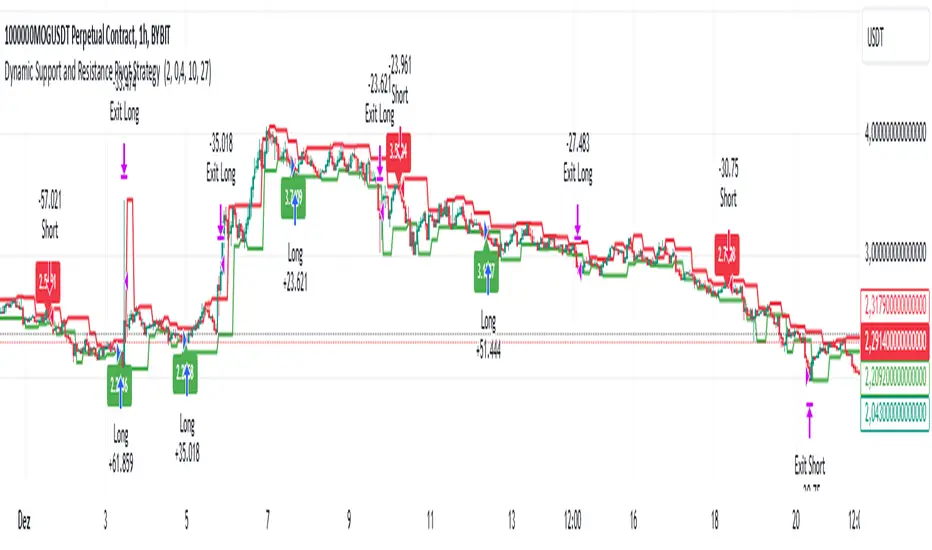
Dynamic Support and Resistance Pivot Strategy The Dynamic Support and Resistance Pivot Strategy is a flexible and adaptive tool designed to identify short-term support and resistance levels using the concept of price pivots.
### Key Elements of the Strategy
1. Pivot points as support and resistance levels
Pivots are significant turning points on the price chart, often marking local highs and lows where the price has reversed direction. A pivot high occurs when the price forms a local peak, while a pivot low occurs when the price forms a local trough. When a new pivot high is formed, it creates a resistance level. Conversely, when a new pivot low is formed, it creates a support level.
The strategy continuously updates these levels as new pivots are detected, ensuring they remain relevant to the current market conditions. By identifying these price levels, the strategy dynamically adjusts to market conditions, allowing it to adapt to both trending and ranging markets, since it has a long target and can perform reversal operations.
2. Entry Criteria
- Buy (Long): A long position is triggered when the price is near the support level and then crosses it from below to above. This suggests that the price has found support and may start moving upwards.
- Sell (Short): A short position is triggered when the price is near the resistance level and then crosses it from above to below. This indicates that the price may be reversing and moving downward.
3. Support/Resistance distance (%)
- This parameter establishes a percentage range around the identified support and resistance level. For example, if the Support Resistance Distance is 0.4% (default), the closing price must be within a range of 0.4% above support or below the resistance to be considered "close" and trigger a trade.
4. Exit criteria
- Take profit = 27 %
- Stop loss = 10 %
- Reversal if a new entry point is identified in the opposite direction
5. No Repainting
- The Dynamic Support and Resistance Pivot Strategy is not subject to repainting.
6. Position Sizing by Equity and risk management
- This strategy has a default configuration to operate with 35% of the equity. The stop loss is set to 10% from the entry price. This way, the strategy is putting at risk about 10% of 35% of equity, that is, around 3.5% of equity for each trade. The percentage of equity and stop loss can be adjusted by the user according to their risk management.
7. Backtest results
- This strategy was subjected to backtest and operations in replay mode on **1000000MOGUSDT.P**, with the inclusion of transaction fees at 0.12% and slipagge of 5 ticks, and the past results have shown consistent profitability. Past results are no guarantee of future results. The strategy's backtest results may even be due to overfitting with past data.
8. Chart Visualization
- Support and resistance levels are displayed as green (support) and red (resistance) lines.
- Pivot prices are displayed as green (pivot low) and red (pivot high) labels.
In this image above, the Support/Resistance distance (%) parameter was set to 0.8.
9. Default Configuration
Chart Timeframe: 1h
Pivot Lengh: 2
Support/Resistance distance (%): 0.4*
Stop Loss: 10 %
Take Profit: 27 %
* This parameter can alternatively be set to 0.8.
10. Alternative Configuration
Chart Timeframe: 20 min
Pivot Lengh: 4
Support/Resistance distance (%): 0.1
Stop Loss: 10 %
Take Profit: 25 %
BYBIT:1000000MOGUSDT.P
Smart Money Breakouts [iskess 01-02 11:05]This is an big update to the excellent Smart Money Breakout Script published in Oct 2023 by ChartPrime who, to my knowledge, was the original author.
FULL CREDIT GOES TO CHARTPRIME FOR THIS ORIGINAL WORK.
Per the moderator's rules, you will find below a meaningful, detailed self-contained description that does not rely on delegation to the open source code or links to other content. You will find in the description details on what the script does, how it does that, how to use it, and how it is original.
The "Smart Money Breakouts" indicator is designed to identify breakouts based on changes in character (CHOCH) or breaks of structure (BOS) patterns, facilitating automated trading with user-defined Take Profit (TP) level.
The indicator incorporates essential elements such as volume analysis and a data table to assist traders in optimizing their strategies.
🔸Breakout Detection:
The indicator scans price movements for "Change in Character" (CHOCH) and "Break of Structure" (BOS) patterns, signaling potential breakout opportunities in the market.
🔸User-Defined TP/SL :
Traders can customize the Take Profit (TP) and Stop Loss (SL) through the indicator settings, with these levels dynamically calculated based on the Average True Range (ATR). This allows for precise risk management and profit targets that adapt to market volatility. Traders can also select the lookback period for the TP/SL calculations.
🔸Volume Analysis and Trade Direction Specific Analysis:
The indicator includes a volume checker that provides valuable insights into the strength of the breakout, taking into account trade direction.
🔸If the volume label is red and the trade is long, it suggests a higher likelihood of hitting the Stop Loss (SL).
🔸If the volume label is green and the trade is long, it indicates a higher probability of hitting the Take Profit (TP).
🔸For short trades, a red volume label suggests a higher likelihood of hitting TP, while a green label suggests a higher likelihood of hitting SL.
🔸A yellow volume label suggests that the volume is inconclusive, neither favoring bullish nor bearish movements.
🔸Data Table:
The indicator features a data table that keeps track of the number of winning and losing trades for specific timeframes or configurations. It also shows the percentage of profits vs losses, and the overall profit/loss for the selected lookback period.
This table serves as a valuable tool for traders to analyze performance and discover optimal settings and timeframes.
The "Smart Money Breakouts" indicator provides traders with a comprehensive solution for breakout trading, combining technical analysis of changes in character and breaks of structure, volume insights, and performance tracking while dynamically adjusting TP and SL levels based on market volatility through the ATR.
This version of the script is a "significant improvement" from Chart Prime's original work in the following ways:
- A selectable range of candles for the profit/loss calculations to look back on.
- An updated table that includes the percentage of wins/losses, and and overall P&L during the selected lookback range.
- The user can now select only Long trades, Short trades, or both.
- The percentage gain/loss is now indicated for every trade on the chart.
- The user can now select a different multiplier for Stop Loss or Take Profit thresholds.

PreannFXExplanation of the PreannFX indicator:
Candle Body Size:
The body of the current candle is larger than the previous candle.
Bullish Engulfing:
The current candle closes higher than the previous candle's high.
The body size is larger than the previous candle.
Bearish Engulfing:
The current candle closes lower than the previous candle's low.
The body size is larger than the previous candle.
Entry and Exit:
Bullish: Enter at the previous candle's open or high, stop loss at the previous low, and take profit is 1:1 with the stop loss.
Bearish: Enter at the previous candle's open or low, stop loss at the previous high, and take profit is 1:1 with the stop loss.
Visualization:
Green upward arrows for bullish engulfing patterns.
Red downward arrows for bearish engulfing patterns.

RISK MANAGEMENT TABLEThis updated Risk Management Indicator is a powerful and customizable tool designed to help traders effectively manage risk on every trade. By dynamically calculating position size, stop-loss, and take-profit levels, it enables traders to stay disciplined and follow predefined risk parameters directly on their charts.
Features:
Dynamic Stop-Loss and Take-Profit Levels:
Stop-loss is based on the Average True Range (ATR), offering a flexible way to account for
market volatility.
Take-profit levels can be customized as a percentage of the entry price, providing a clear
target for trade exits.
Position Sizing Calculation:
The indicator computes the maximum position size by considering:
Trade amount (montant_ligne).
Risk percentage per trade.
Transaction fees.
Visual Representation:
Displays stop-loss and take-profit levels on the chart as customizable lines.
Optional visibility of these lines through checkboxes in the settings panel.
Comprehensive Risk Table:
A table on the chart summarizes essential risk metrics:
Stop-loss value.
Distance from entry in percentage.
Position size (maximum suggested).
Take-profit price.
Customizable:
Adjust parameters like ATR length, smoothing type, risk percentage, transaction fees,
and take-profit percentage.
Modify the visual length of lines representing stop-loss and take-profit levels.
How It Works:
Stop-Loss Calculation:
The stop-loss level is calculated using ATR and a volatility factor (default: 2).
This ensures your stop-loss adapts to market conditions.
Take-Profit Calculation:
Take-profit is derived as a percentage increase from the entry price.
Position Size:
The optimal position size is computed as:
Position Size = Risk per Trade /ATR-based Stop Distance
The risk per trade deducts transaction fees to provide a more accurate calculation.
Visual Lines:
Risk Table:
The table displays updated stop-loss, position size, and take-profit metrics at a glance.
Settings Panel:
Length: ATR length for calculating market volatility.
Smoothing: Choose RMA, SMA, EMA, or WMA for ATR smoothing.
Trade Amount: The capital allocated to a single trade.
Risk by Trade (%): Define how much of your trade capital is at risk per trade.
Transaction Fees: Input fees to ensure realistic calculations.
Take Profit (%): Specify your desired take-profit percentage.
Show Entry Stop Loss: Toggle visibility of the stop-loss line.
Show Entry Take Profit: Toggle visibility of the take-profit line.

Filtered ATR with EMA OverlayFiltered ATR with EMA Overlay is an advanced volatility indicator designed to provide a more accurate representation of market conditions by smoothing the standard Average True Range (ATR). This is achieved by filtering out extreme price movements and abnormal bars that can distort traditional ATR calculations.
The indicator applies an Exponential Moving Average (EMA) to the filtered ATR, creating a dual-layered system that highlights periods of increased or decreased volatility.
Key Features:
Filtered ATR: Filters out extreme bars, reducing noise and making the ATR line more reliable.
EMA Overlay: An EMA (default period of 10) is applied to the filtered ATR, allowing traders to track average volatility trends.
Volatility Signals:
Filtered ATR > EMA(10): Indicates higher-than-average volatility. This often correlates with trend breakouts or strong price movements.
Filtered ATR < EMA(10): Suggests reduced volatility, signaling potential consolidation or sideways price action.
Parameters:
atrLength (Default: 5):
The number of bars used to calculate the ATR. A shorter period (e.g., 3-5) responds faster to price changes, while a longer period (e.g., 10-14) provides smoother results.
multiplier (Default: 1.8):
Controls the sensitivity of the filter. A lower multiplier (e.g., 1.5) filters out more bars, resulting in smoother ATR. Higher values (e.g., 2.0) allow more bars to pass through, retaining more price volatility.
maxIterations (Default: 20):
The maximum number of bars processed to detect abnormal values. Increasing this may improve accuracy at the cost of performance.
ema10Period (Default: 10):
The period for the Exponential Moving Average applied to the filtered ATR. Shorter periods provide faster signals, while longer periods give smoother, lagging signals.
Trading Strategies:
1. Breakout Strategy:
When filtered ATR crosses above EMA(10):
Enter long positions when price breaks above a key resistance level.
Higher volatility suggests strong price action and momentum.
When filtered ATR drops below EMA(10):
Exit positions or tighten stop-loss orders as volatility decreases.
Lower volatility may indicate consolidation or trend exhaustion.
2. Trend Following Strategy:
Use the filtered ATR line to track overall volatility.
If filtered ATR consistently stays above EMA: Hold positions or add to trades.
If filtered ATR remains below EMA: Reduce position size or stay out of trades.
3. Mean Reversion Strategy:
When filtered ATR spikes significantly above EMA, it may indicate market overreaction.
Look for price to revert to the mean once ATR returns below the EMA.
4. Stop-Loss Adjustment:
As volatility increases (ATR above EMA), widen stop-loss levels to avoid being stopped out by random fluctuations.
In low volatility (ATR below EMA), tighten stop-losses to minimize losses during low activity periods.
Benefits:
Reduced Noise: By filtering abnormal bars, the indicator provides cleaner signals.
Better Trend Detection: EMA smoothing highlights volatility trends.
Adaptable: The indicator can be customized for scalping, day trading, or swing trading.
Intuitive Visualization: Traders can visually see volatility shifts and adjust strategies in real-time.
Best Practices:
Timeframes: Works effectively on all timeframes, but higher timeframes (e.g., 1H, 4H, Daily) yield more reliable signals.
Markets: Suitable for forex, crypto, stocks, and commodities.
Combining Indicators: Use in combination with RSI, Moving Averages, Bollinger Bands, or price action analysis for stronger signals.
How It Works (Under the Hood):
The script calculates the Daily Range (High - Low) for each bar.
The largest and smallest bars are filtered out if their difference exceeds the multiplier (default 1.8).
The remaining bars are averaged to generate the filtered ATR.
An EMA(10) is then applied to the filtered ATR for smoother visualization.

Wave Surge [UAlgo]The "Wave Surge " is a comprehensive indicator designed to provide advanced wave pattern analysis for market trends and price movements. Built with customizable parameters, it caters to both beginner and advanced traders looking to improve their decision-making process.
This indicator utilizes wave-based calculations, adaptive thresholds, and volume analysis to detect and visualize key market signals. By integrating multiple analysis techniques.
It calculates waves for high, low, and close prices using a configurable moving average (EMA) technique and pairs it with volume and baseline analysis to confirm patterns. The result is a robust framework for identifying potential entry and exit points in the market.
🔶 Key Features
Wave-Based Analysis: This indicator computes waves using exponential moving averages (EMA) of high, low, and close prices, with an adjustable wave period to suit different market conditions.
Customizable Baseline: Traders can select from multiple baseline types, including VWMA (Volume-Weighted Moving Average), EMA, SMA (Simple Moving Average), and HMA (Hull Moving Average), for trend confirmation.
Adaptive Thresholds: The adaptive threshold feature dynamically adjusts sensitivity based on a chosen period, ensuring the indicator remains responsive to varying market volatility.
Volume Analysis: The integrated volume analysis calculates volume ratios and allows traders to enable or disable this feature to refine signal accuracy.
Pattern Recognition: The indicator identifies specific wave patterns (Wave 1, Wave 3, Wave 4, Wave 5, Wave 6) and visually plots them on the chart for easy interpretation.
Visual and Color-Coded Signals: Clear visual signals (upward and downward arrows) are plotted on the chart to highlight potential bullish or bearish patterns. The baseline is color-coded for an intuitive understanding of market trends.
Configuration: Parameters for wave period, baseline length, volume factors, and sensitivity can be tailored to align with the trader’s strategy and market environment.
🔶 Interpreting the Indicator
Wave Patterns
The indicator detects and plots six unique wave patterns based on price changes that exceed an adaptive threshold. These patterns are validated by the direction of the baseline:
Wave 1 (Bullish): Triggered when the price increases above the threshold while the baseline is falling.
Wave 3, 4, and 6 (Bearish): Indicate potential downtrends validated by a rising baseline.
Wave 5 (Bullish): Suggests upward momentum when prices exceed the threshold with a falling baseline.
Baseline Trend
The baseline serves as a trend confirmation tool, dynamically changing color to reflect market direction:
Aqua (Rising): Indicates an upward trend.
Red (Falling): Indicates a downward trend.
Volume Confirmation
When enabled, the volume analysis feature ensures that signals are supported by significant volume movements. Patterns with high volume are considered more reliable.
Signal Visualization
Upward Arrows (🡹): Highlight potential bullish opportunities.
Downward Arrows (🡻): Highlight potential bearish opportunities.
Alerts
Alerts are triggered when key wave patterns are identified, providing traders with timely notifications to take action without being tied to the screen.
🔶 Disclaimer
Use with Caution: This indicator is provided for educational and informational purposes only and should not be considered as financial advice. Users should exercise caution and perform their own analysis before making trading decisions based on the indicator's signals.
Not Financial Advice: The information provided by this indicator does not constitute financial advice, and the creator (UAlgo) shall not be held responsible for any trading losses incurred as a result of using this indicator.
Backtesting Recommended: Traders are encouraged to backtest the indicator thoroughly on historical data before using it in live trading to assess its performance and suitability for their trading strategies.
Risk Management: Trading involves inherent risks, and users should implement proper risk management strategies, including but not limited to stop-loss orders and position sizing, to mitigate potential losses.
No Guarantees: The accuracy and reliability of the indicator's signals cannot be guaranteed, as they are based on historical price data and past performance may not be indicative of future results.

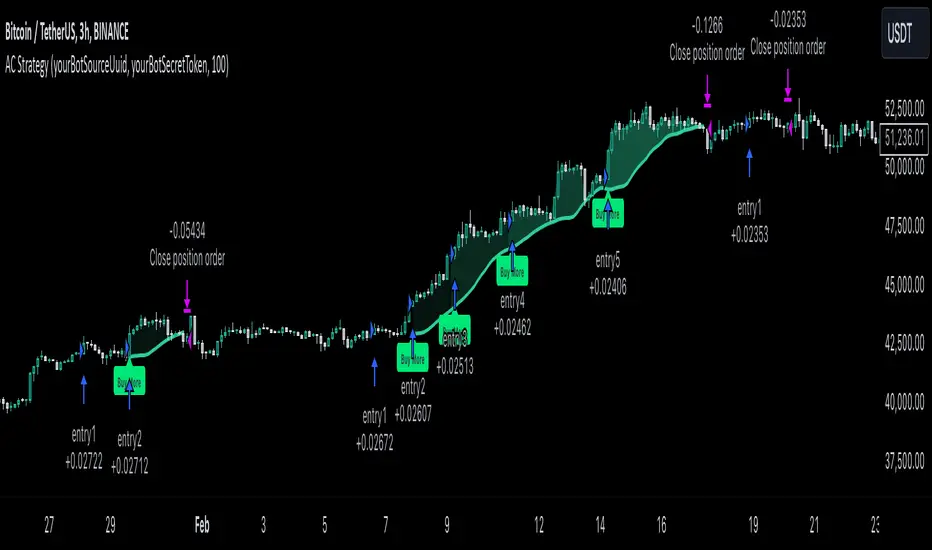
MultiLayer Acceleration/Deceleration Strategy [Skyrexio]Overview
MultiLayer Acceleration/Deceleration Strategy leverages the combination of Acceleration/Deceleration Indicator(AC), Williams Alligator, Williams Fractals and Exponential Moving Average (EMA) to obtain the high probability long setups. Moreover, strategy uses multi trades system, adding funds to long position if it considered that current trend has likely became stronger. Acceleration/Deceleration Indicator is used for creating signals, while Alligator and Fractal are used in conjunction as an approximation of short-term trend to filter them. At the same time EMA (default EMA's period = 100) is used as high probability long-term trend filter to open long trades only if it considers current price action as an uptrend. More information in "Methodology" and "Justification of Methodology" paragraphs. The strategy opens only long trades.
Unique Features
No fixed stop-loss and take profit: Instead of fixed stop-loss level strategy utilizes technical condition obtained by Fractals and Alligator to identify when current uptrend is likely to be over (more information in "Methodology" and "Justification of Methodology" paragraphs)
Configurable Trading Periods: Users can tailor the strategy to specific market windows, adapting to different market conditions.
Multilayer trades opening system: strategy uses only 10% of capital in every trade and open up to 5 trades at the same time if script consider current trend as strong one.
Short and long term trend trade filters: strategy uses EMA as high probability long-term trend filter and Alligator and Fractal combination as a short-term one.
Methodology
The strategy opens long trade when the following price met the conditions:
1. Price closed above EMA (by default, period = 100). Crossover is not obligatory.
2. Combination of Alligator and Williams Fractals shall consider current trend as an upward (all details in "Justification of Methodology" paragraph)
3. Acceleration/Deceleration shall create one of two types of long signals (all details in "Justification of Methodology" paragraph). Buy stop order is placed one tick above the candle's high of last created long signal.
4. If price reaches the order price, long position is opened with 10% of capital.
5. If currently we have opened position and price creates and hit the order price of another one long signal, another one long position will be added to the previous with another one 10% of capital. Strategy allows to open up to 5 long trades simultaneously.
6. If combination of Alligator and Williams Fractals shall consider current trend has been changed from up to downtrend, all long trades will be closed, no matter how many trades has been opened.
Script also has additional visuals. If second long trade has been opened simultaneously the Alligator's teeth line is plotted with the green color. Also for every trade in a row from 2 to 5 the label "Buy More" is also plotted just below the teeth line. With every next simultaneously opened trade the green color of the space between teeth and price became less transparent.
Strategy settings
In the inputs window user can setup strategy setting: EMA Length (by default = 100, period of EMA, used for long-term trend filtering EMA calculation). User can choose the optimal parameters during backtesting on certain price chart.
Justification of Methodology
Let's explore the key concepts of this strategy and understand how they work together. We'll begin with the simplest: the EMA.
The Exponential Moving Average (EMA) is a type of moving average that assigns greater weight to recent price data, making it more responsive to current market changes compared to the Simple Moving Average (SMA). This tool is widely used in technical analysis to identify trends and generate buy or sell signals. The EMA is calculated as follows:
1.Calculate the Smoothing Multiplier:
Multiplier = 2 / (n + 1), Where n is the number of periods.
2. EMA Calculation
EMA = (Current Price) × Multiplier + (Previous EMA) × (1 − Multiplier)
In this strategy, the EMA acts as a long-term trend filter. For instance, long trades are considered only when the price closes above the EMA (default: 100-period). This increases the likelihood of entering trades aligned with the prevailing trend.
Next, let’s discuss the short-term trend filter, which combines the Williams Alligator and Williams Fractals. Williams Alligator
Developed by Bill Williams, the Alligator is a technical indicator that identifies trends and potential market reversals. It consists of three smoothed moving averages:
Jaw (Blue Line): The slowest of the three, based on a 13-period smoothed moving average shifted 8 bars ahead.
Teeth (Red Line): The medium-speed line, derived from an 8-period smoothed moving average shifted 5 bars forward.
Lips (Green Line): The fastest line, calculated using a 5-period smoothed moving average shifted 3 bars forward.
When the lines diverge and align in order, the "Alligator" is "awake," signaling a strong trend. When the lines overlap or intertwine, the "Alligator" is "asleep," indicating a range-bound or sideways market. This indicator helps traders determine when to enter or avoid trades.
Fractals, another tool by Bill Williams, help identify potential reversal points on a price chart. A fractal forms over at least five consecutive bars, with the middle bar showing either:
Up Fractal: Occurs when the middle bar has a higher high than the two preceding and two following bars, suggesting a potential downward reversal.
Down Fractal: Happens when the middle bar shows a lower low than the surrounding two bars, hinting at a possible upward reversal.
Traders often use fractals alongside other indicators to confirm trends or reversals, enhancing decision-making accuracy.
How do these tools work together in this strategy? Let’s consider an example of an uptrend.
When the price breaks above an up fractal, it signals a potential bullish trend. This occurs because the up fractal represents a shift in market behavior, where a temporary high was formed due to selling pressure. If the price revisits this level and breaks through, it suggests the market sentiment has turned bullish.
The breakout must occur above the Alligator’s teeth line to confirm the trend. A breakout below the teeth is considered invalid, and the downtrend might still persist. Conversely, in a downtrend, the same logic applies with down fractals.
In this strategy if the most recent up fractal breakout occurs above the Alligator's teeth and follows the last down fractal breakout below the teeth, the algorithm identifies an uptrend. Long trades can be opened during this phase if a signal aligns. If the price breaks a down fractal below the teeth line during an uptrend, the strategy assumes the uptrend has ended and closes all open long trades.
By combining the EMA as a long-term trend filter with the Alligator and fractals as short-term filters, this approach increases the likelihood of opening profitable trades while staying aligned with market dynamics.
Now let's talk about Acceleration/Deceleration signals. AC indicator is calculated using the Awesome Oscillator, so let's first of all briefly explain what is Awesome Oscillator and how it can be calculated. The Awesome Oscillator (AO), developed by Bill Williams, is a momentum indicator designed to measure market momentum by contrasting recent price movements with a longer-term historical perspective. It helps traders detect potential trend reversals and assess the strength of ongoing trends.
The formula for AO is as follows:
AO = SMA5(Median Price) − SMA34(Median Price)
where:
Median Price = (High + Low) / 2
SMA5 = 5-period Simple Moving Average of the Median Price
SMA 34 = 34-period Simple Moving Average of the Median Price
The Acceleration/Deceleration (AC) Indicator, introduced by Bill Williams, measures the rate of change in market momentum. It highlights shifts in the driving force of price movements and helps traders spot early signs of trend changes. The AC Indicator is particularly useful for identifying whether the current momentum is accelerating or decelerating, which can indicate potential reversals or continuations. For AC calculation we shall use the AO calculated above is the following formula:
AC = AO − SMA5(AO), where SMA5(AO)is the 5-period Simple Moving Average of the Awesome Oscillator
When the AC is above the zero line and rising, it suggests accelerating upward momentum.
When the AC is below the zero line and falling, it indicates accelerating downward momentum.
When the AC is below zero line and rising it suggests the decelerating the downtrend momentum. When AC is above the zero line and falling, it suggests the decelerating the uptrend momentum.
Now we can explain which AC signal types are used in this strategy. The first type of long signal is when AC value is below zero line. In this cases we need to see three rising bars on the histogram in a row after the falling one. The second type of signals occurs above the zero line. There we need only two rising AC bars in a row after the falling one to create the signal. The signal bar is the last green bar in this sequence. The strategy places the buy stop order one tick above the candle's high, which corresponds to the signal bar on AC indicator.
After that we can have the following scenarios:
Price hit the order on the next candle in this case strategy opened long with this price.
Price doesn't hit the order price, the next candle set lower high. If current AC bar is increasing buy stop order changes by the script to the high of this new bar plus one tick. This procedure repeats until price finally hit buy order or current AC bar become decreasing. In the second case buy order cancelled and strategy wait for the next AC signal.
If long trades are initiated, the strategy continues utilizing subsequent signals until the total number of trades reaches a maximum of 5. All open trades are closed when the trend shifts to a downtrend, as determined by the combination of the Alligator and Fractals described earlier.
Why we use AC signals? If currently strategy algorithm considers the high probability of the short-term uptrend with the Alligator and Fractals combination pointed out above and the long-term trend is also suggested by the EMA filter as bullish. Rising AC bars after period of falling AC bars indicates the high probability of local pull back end and there is a high chance to open long trade in the direction of the most likely main uptrend. The numbers of rising bars are different for the different AC values (below or above zero line). This is needed because if AC below zero line the local downtrend is likely to be stronger and needs more rising bars to confirm that it has been changed than if AC is above zero.
Why strategy use only 10% per signal? Sometimes we can see the false signals which appears on sideways. Not risking that much script use only 10% per signal. If the first long trade has been open and price continue going up and our trend approximation by Alligator and Fractals is uptrend, strategy add another one 10% of capital to every next AC signal while number of active trades no more than 5. This capital allocation allows to take part in long trades when current uptrend is likely to be strong and use only 10% of capital when there is a high probability of sideways.
Backtest Results
Operating window: Date range of backtests is 2023.01.01 - 2024.11.01. It is chosen to let the strategy to close all opened positions.
Commission and Slippage: Includes a standard Binance commission of 0.1% and accounts for possible slippage over 5 ticks.
Initial capital: 10000 USDT
Percent of capital used in every trade: 10%
Maximum Single Position Loss: -5.15%
Maximum Single Profit: +24.57%
Net Profit: +2108.85 USDT (+21.09%)
Total Trades: 111 (36.94% win rate)
Profit Factor: 2.391
Maximum Accumulated Loss: 367.61 USDT (-2.97%)
Average Profit per Trade: 19.00 USDT (+1.78%)
Average Trade Duration: 75 hours
How to Use
Add the script to favorites for easy access.
Apply to the desired timeframe and chart (optimal performance observed on 3h BTC/USDT).
Configure settings using the dropdown choice list in the built-in menu.
Set up alerts to automate strategy positions through web hook with the text: {{strategy.order.alert_message}}
Disclaimer:
Educational and informational tool reflecting Skyrex commitment to informed trading. Past performance does not guarantee future results. Test strategies in a simulated environment before live implementation
These results are obtained with realistic parameters representing trading conditions observed at major exchanges such as Binance and with realistic trading portfolio usage parameters.
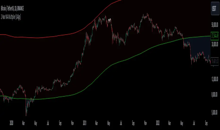
2-Year MA Multiplier [UAlgo]The 2-Year MA Multiplier is a technical analysis tool designed to assist traders and investors in identifying potential overbought and oversold conditions in the market. By plotting the 2-year moving average (MA) of an asset's closing price alongside an upper band set at five times this moving average, the indicator provides visual cues to assess long-term price trends and significant market movements.
🔶 Key Features
2-Year Moving Average (MA): Calculates the simple moving average of the asset's closing price over a 730-day period, representing approximately two years.
Visual Indicators: Plots the 2-year MA in forest green and the upper band in firebrick red for clear differentiation.
Fills the area between the 2-year MA and the upper band to highlight the normal trading range.
Uses color-coded fills to indicate overbought (tomato red) and oversold (cornflower blue) conditions based on the asset's closing price relative to the bands.
🔶 Idea
The concept behind the 2-Year MA Multiplier is rooted in the cyclical nature of markets, particularly in assets like Bitcoin. By analyzing long-term price movements, the indicator aims to identify periods of significant deviation from the norm, which may signal potential buying or selling opportunities.
2-year MA smooths out short-term volatility, providing a clearer view of the asset's long-term trend. This timeframe is substantial enough to capture major market cycles, making it a reliable baseline for analysis.
Multiplying the 2-year MA by five establishes an upper boundary that has historically correlated with market tops. When the asset's price exceeds this upper band, it may indicate overbought conditions, suggesting a potential for price correction. Conversely, when the price falls below the 2-year MA, it may signal oversold conditions, presenting potential buying opportunities.
🔶 Disclaimer
Use with Caution: This indicator is provided for educational and informational purposes only and should not be considered as financial advice. Users should exercise caution and perform their own analysis before making trading decisions based on the indicator's signals.
Not Financial Advice: The information provided by this indicator does not constitute financial advice, and the creator (UAlgo) shall not be held responsible for any trading losses incurred as a result of using this indicator.
Backtesting Recommended: Traders are encouraged to backtest the indicator thoroughly on historical data before using it in live trading to assess its performance and suitability for their trading strategies.
Risk Management: Trading involves inherent risks, and users should implement proper risk management strategies, including but not limited to stop-loss orders and position sizing, to mitigate potential losses.
No Guarantees: The accuracy and reliability of the indicator's signals cannot be guaranteed, as they are based on historical price data and past performance may not be indicative of future results.
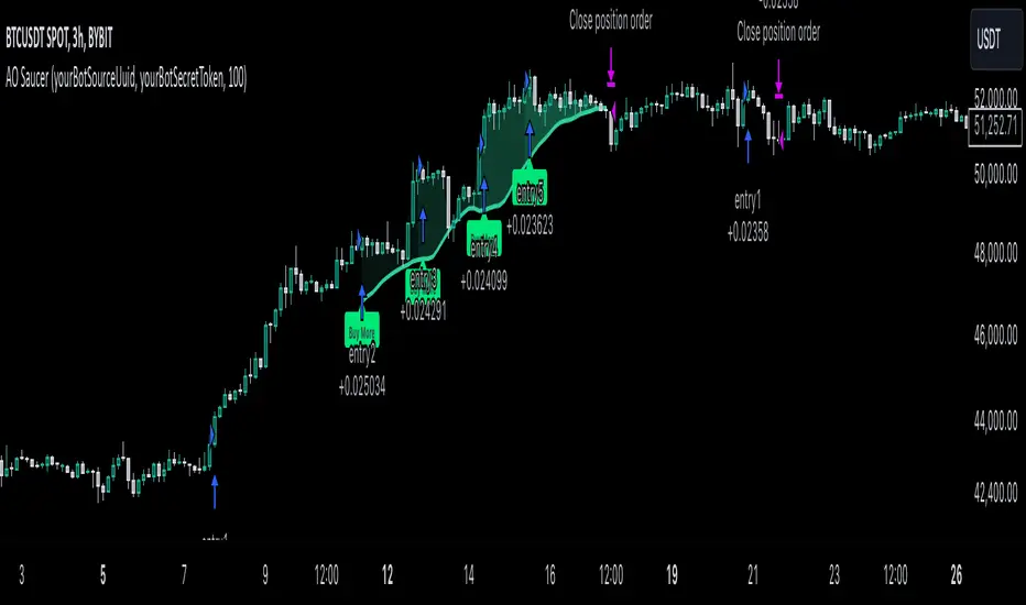
MultiLayer Awesome Oscillator Saucer Strategy [Skyrexio]Overview
MultiLayer Awesome Oscillator Saucer Strategy leverages the combination of Awesome Oscillator (AO), Williams Alligator, Williams Fractals and Exponential Moving Average (EMA) to obtain the high probability long setups. Moreover, strategy uses multi trades system, adding funds to long position if it considered that current trend has likely became stronger. Awesome Oscillator is used for creating signals, while Alligator and Fractal are used in conjunction as an approximation of short-term trend to filter them. At the same time EMA (default EMA's period = 100) is used as high probability long-term trend filter to open long trades only if it considers current price action as an uptrend. More information in "Methodology" and "Justification of Methodology" paragraphs. The strategy opens only long trades.
Unique Features
No fixed stop-loss and take profit: Instead of fixed stop-loss level strategy utilizes technical condition obtained by Fractals and Alligator to identify when current uptrend is likely to be over (more information in "Methodology" and "Justification of Methodology" paragraphs)
Configurable Trading Periods: Users can tailor the strategy to specific market windows, adapting to different market conditions.
Multilayer trades opening system: strategy uses only 10% of capital in every trade and open up to 5 trades at the same time if script consider current trend as strong one.
Short and long term trend trade filters: strategy uses EMA as high probability long-term trend filter and Alligator and Fractal combination as a short-term one.
Methodology
The strategy opens long trade when the following price met the conditions:
1. Price closed above EMA (by default, period = 100). Crossover is not obligatory.
2. Combination of Alligator and Williams Fractals shall consider current trend as an upward (all details in "Justification of Methodology" paragraph)
3. Awesome Oscillator shall create the "Saucer" long signal (all details in "Justification of Methodology" paragraph). Buy stop order is placed one tick above the candle's high of last created "Saucer signal".
4. If price reaches the order price, long position is opened with 10% of capital.
5. If currently we have opened position and price creates and hit the order price of another one "Saucer" signal another one long position will be added to the previous with another one 10% of capital. Strategy allows to open up to 5 long trades simultaneously.
6. If combination of Alligator and Williams Fractals shall consider current trend has been changed from up to downtrend, all long trades will be closed, no matter how many trades has been opened.
Script also has additional visuals. If second long trade has been opened simultaneously the Alligator's teeth line is plotted with the green color. Also for every trade in a row from 2 to 5 the label "Buy More" is also plotted just below the teeth line. With every next simultaneously opened trade the green color of the space between teeth and price became less transparent.
Strategy settings
In the inputs window user can setup strategy setting: EMA Length (by default = 100, period of EMA, used for long-term trend filtering EMA calculation). User can choose the optimal parameters during backtesting on certain price chart.
Justification of Methodology
Let's go through all concepts used in this strategy to understand how they works together. Let's start from the easies one, the EMA. Let's briefly explain what is EMA. The Exponential Moving Average (EMA) is a type of moving average that gives more weight to recent prices, making it more responsive to current price changes compared to the Simple Moving Average (SMA). It is commonly used in technical analysis to identify trends and generate buy or sell signals. It can be calculated with the following steps:
1.Calculate the Smoothing Multiplier:
Multiplier = 2 / (n + 1), Where n is the number of periods.
2. EMA Calculation
EMA = (Current Price) × Multiplier + (Previous EMA) × (1 − Multiplier)
In this strategy uses EMA an initial long term trend filter. It allows to open long trades only if price close above EMA (by default 50 period). It increases the probability of taking long trades only in the direction of the trend.
Let's go to the next, short-term trend filter which consists of Alligator and Fractals. Let's briefly explain what do these indicators means. The Williams Alligator, developed by Bill Williams, is a technical indicator designed to spot trends and potential market reversals. It uses three smoothed moving averages, referred to as the jaw, teeth, and lips:
Jaw (Blue Line): The slowest of the three, based on a 13-period smoothed moving average shifted 8 bars ahead.
Teeth (Red Line): The medium-speed line, derived from an 8-period smoothed moving average shifted 5 bars forward.
Lips (Green Line): The fastest line, calculated using a 5-period smoothed moving average shifted 3 bars forward.
When these lines diverge and are properly aligned, the "alligator" is considered "awake," signaling a strong trend. Conversely, when the lines overlap or intertwine, the "alligator" is "asleep," indicating a range-bound or sideways market. This indicator assists traders in identifying when to act on or avoid trades.
The Williams Fractals, another tool introduced by Bill Williams, are used to pinpoint potential reversal points on a price chart. A fractal forms when there are at least five consecutive bars, with the middle bar displaying the highest high (for an up fractal) or the lowest low (for a down fractal), relative to the two bars on either side.
Key Points:
Up Fractal: Occurs when the middle bar has a higher high than the two preceding and two following bars, suggesting a potential downward reversal.
Down Fractal: Happens when the middle bar shows a lower low than the surrounding two bars, hinting at a possible upward reversal.
Traders often combine fractals with other indicators to confirm trends or reversals, improving the accuracy of trading decisions.
How we use their combination in this strategy? Let’s consider an uptrend example. A breakout above an up fractal can be interpreted as a bullish signal, indicating a high likelihood that an uptrend is beginning. Here's the reasoning: an up fractal represents a potential shift in market behavior. When the fractal forms, it reflects a pullback caused by traders selling, creating a temporary high. However, if the price manages to return to that fractal’s high and break through it, it suggests the market has "changed its mind" and a bullish trend is likely emerging.
The moment of the breakout marks the potential transition to an uptrend. It’s crucial to note that this breakout must occur above the Alligator's teeth line. If it happens below, the breakout isn’t valid, and the downtrend may still persist. The same logic applies inversely for down fractals in a downtrend scenario.
So, if last up fractal breakout was higher, than Alligator's teeth and it happened after last down fractal breakdown below teeth, algorithm considered current trend as an uptrend. During this uptrend long trades can be opened if signal was flashed. If during the uptrend price breaks down the down fractal below teeth line, strategy considered that uptrend is finished with the high probability and strategy closes all current long trades. This combination is used as a short term trend filter increasing the probability of opening profitable long trades in addition to EMA filter, described above.
Now let's talk about Awesome Oscillator's "Sauser" signals. Briefly explain what is the Awesome Oscillator. The Awesome Oscillator (AO), created by Bill Williams, is a momentum-based indicator that evaluates market momentum by comparing recent price activity to a broader historical context. It assists traders in identifying potential trend reversals and gauging trend strength.
AO = SMA5(Median Price) − SMA34(Median Price)
where:
Median Price = (High + Low) / 2
SMA5 = 5-period Simple Moving Average of the Median Price
SMA 34 = 34-period Simple Moving Average of the Median Price
Now we know what is AO, but what is the "Saucer" signal? This concept was introduced by Bill Williams, let's briefly explain it and how it's used by this strategy. Initially, this type of signal is a combination of the following AO bars: we need 3 bars in a row, the first one shall be higher than the second, the third bar also shall be higher, than second. All three bars shall be above the zero line of AO. The price bar, which corresponds to third "saucer's" bar is our signal bar. Strategy places buy stop order one tick above the price bar which corresponds to signal bar.
After that we can have the following scenarios.
Price hit the order on the next candle in this case strategy opened long with this price.
Price doesn't hit the order price, the next candle set lower low. If current AO bar is increasing buy stop order changes by the script to the high of this new bar plus one tick. This procedure repeats until price finally hit buy order or current AO bar become decreasing. In the second case buy order cancelled and strategy wait for the next "Saucer" signal.
If long trades has been opened strategy use all the next signals until number of trades doesn't exceed 5. All trades are closed when the trend changes to downtrend according to combination of Alligator and Fractals described above.
Why we use "Saucer" signals? If AO above the zero line there is a high probability that price now is in uptrend if we take into account our two trend filters. When we see the decreasing bars on AO and it's above zero it's likely can be considered as a pullback on the uptrend. When we see the stop of AO decreasing and the first increasing bar has been printed there is a high probability that this local pull back is finished and strategy open long trade in the likely direction of a main trend.
Why strategy use only 10% per signal? Sometimes we can see the false signals which appears on sideways. Not risking that much script use only 10% per signal. If the first long trade has been open and price continue going up and our trend approximation by Alligator and Fractals is uptrend, strategy add another one 10% of capital to every next saucer signal while number of active trades no more than 5. This capital allocation allows to take part in long trades when current uptrend is likely to be strong and use only 10% of capital when there is a high probability of sideways.
Backtest Results
Operating window: Date range of backtests is 2023.01.01 - 2024.11.25. It is chosen to let the strategy to close all opened positions.
Commission and Slippage: Includes a standard Binance commission of 0.1% and accounts for possible slippage over 5 ticks.
Initial capital: 10000 USDT
Percent of capital used in every trade: 10%
Maximum Single Position Loss: -5.10%
Maximum Single Profit: +22.80%
Net Profit: +2838.58 USDT (+28.39%)
Total Trades: 107 (42.99% win rate)
Profit Factor: 3.364
Maximum Accumulated Loss: 373.43 USDT (-2.98%)
Average Profit per Trade: 26.53 USDT (+2.40%)
Average Trade Duration: 78 hours
These results are obtained with realistic parameters representing trading conditions observed at major exchanges such as Binance and with realistic trading portfolio usage parameters.
How to Use
Add the script to favorites for easy access.
Apply to the desired timeframe and chart (optimal performance observed on 3h BTC/USDT).
Configure settings using the dropdown choice list in the built-in menu.
Set up alerts to automate strategy positions through web hook with the text: {{strategy.order.alert_message}}
Disclaimer:
Educational and informational tool reflecting Skyrex commitment to informed trading. Past performance does not guarantee future results. Test strategies in a simulated environment before live implementation
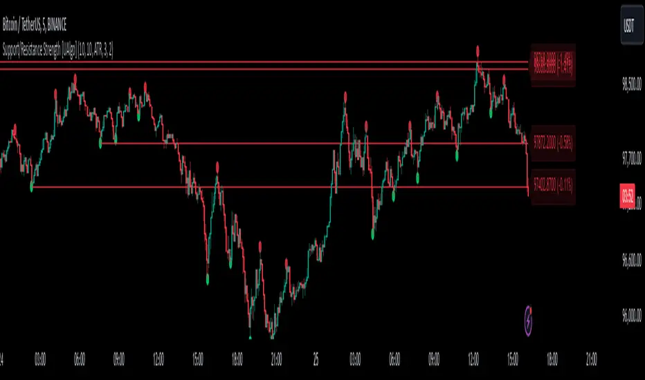
Support/Resistance Strength [UAlgo]The Support/Resistance Strength indicator is a tool designed for traders seeking a precise understanding of key support and resistance levels in the market. This tool dynamically identifies and visualizes support and resistance zones based on pivot points and strength criteria, providing traders with actionable insights for better decision-making.
By incorporating features such as ATR-based or percentage-based channel calculations, customizable strength thresholds, and intuitive visualization of key levels, the indicator caters to traders of various skill levels and strategies. It also adapts dynamically to market conditions, allowing users to identify frequently tested zones with minimal manual input.
🔶 Key Features
Dynamic Support and Resistance Zones
Automatically detects significant support and resistance levels using pivot high and low calculations.
Offers ATR-based or percentage-based channel customization to cater to diverse trading styles.
Customizable Parameters
Lookback period for pivot calculations, strength threshold, and maximum stored pivots are fully adjustable.
Display options for showing specific numbers of recent support/resistance lines.
Intuitive Visualization
Highlights key support and resistance levels with color-coded lines and labels.
Includes percentage deviation from the current price for quick assessment.
Interactive Updates
Continuously updates support and resistance levels to reflect changing market dynamics.
Displays pivot points visually for enhanced clarity.
Can be used effectively on various timeframes, from intraday to daily and weekly charts.
🔶 Interpreting the Indicator
Identifying Key Levels
Support levels are indicated by green (lime) lines and resistance levels by red lines. The transparency of colors is adjustable for visual preference.
Labels display the exact price level and the percentage difference from the current price.
Strength Threshold
The "Minimum S/R Strength" parameter defines how frequently a level must be tested to be considered significant.
Higher strength values indicate zones that have been tested more frequently, suggesting stronger support or resistance.
Pivot Points
The indicator marks pivot high and low points on the chart to provide a visual representation of the calculated levels.
Dynamic Updates
The indicator adapts to the most recent price action. If the price moves above a resistance level or below a support level, the color of the lines and labels will dynamically change to reflect the current price positioning.
🔶 Disclaimer
Use with Caution: This indicator is provided for educational and informational purposes only and should not be considered as financial advice. Users should exercise caution and perform their own analysis before making trading decisions based on the indicator's signals.
Not Financial Advice: The information provided by this indicator does not constitute financial advice, and the creator (UAlgo) shall not be held responsible for any trading losses incurred as a result of using this indicator.
Backtesting Recommended: Traders are encouraged to backtest the indicator thoroughly on historical data before using it in live trading to assess its performance and suitability for their trading strategies.
Risk Management: Trading involves inherent risks, and users should implement proper risk management strategies, including but not limited to stop-loss orders and position sizing, to mitigate potential losses.
No Guarantees: The accuracy and reliability of the indicator's signals cannot be guaranteed, as they are based on historical price data and past performance may not be indicative of future results.
16. SMC Strategy with SL - low TimeframeOverview
The "SMC Strategy with SL - low Timeframe" is a comprehensive trading strategy that uses key concepts from Smart Money Theory to identify favorable areas in the market for buying or selling. This strategy takes advantage of price imbalances, support and resistance zones, and swing highs/lows to generate high-probability trade signals.
The key features of this strategy include:
Swing High/Low Analysis: Used to determine the Premium, Equilibrium, and Discount Zones.
Order Block Integration: An added layer of confluence to identify valid buy and sell signals.
Trend Direction Confirmation: Using a Simple Moving Average (SMA) to determine the overall trend.
Entry and Exit Rules: Based on price position relative to key zones and moving average, along with optional stop-loss and take-profit levels.
Detailed Description
Swing High and Swing Low Analysis
The script calculates Swing High and Swing Low based on the most recent price highs and lows over a specified look-back period (swingHighLength and swingLowLength, set to 8 by default).
It then derives the Premium, Equilibrium, and Discount Zones:
Premium Zone: Represents potential resistance, calculated based on recent swing highs.
Discount Zone: Represents potential support, calculated based on recent swing lows.
Equilibrium: The midpoint between Swing High and Swing Low, dividing the price range into Premium (above equilibrium) and Discount (below equilibrium) areas.
Zone Visualization
The strategy plots the Premium Zone (resistance) in red, the Discount Zone (support) in green, and the Equilibrium level in blue on the chart. This helps visually assess the current price relative to these important areas.
Simple Moving Average (SMA)
A 50-period Simple Moving Average (SMA) is added to help identify the trend direction.
Buy signals are valid only if the price is above the SMA, indicating an uptrend.
Sell signals are valid only if the price is below the SMA, indicating a downtrend.
Entry Rules
The script generates buy or sell signals when certain conditions are met:
A buy signal is triggered when:
Price is below the Equilibrium and within the Discount Zone.
Price is above the SMA.
The buy signal is further confirmed by the presence of an Order Block (recent lowest price area).
A sell signal is triggered when:
Price is above the Equilibrium and within the Premium Zone.
Price is below the SMA.
The sell signal is further confirmed by the presence of an Order Block (recent highest price area).
Order Block
The strategy defines Order Blocks as recent highs and lows within a look-back period (orderBlockLength set to 20 by default).
These blocks represent areas where large players (smart money) have historically been active, increasing the probability of the price reacting in these areas again.
Trade Management and Trade Direction
The user can set Trade Direction to either "Long Only," "Short Only," or "Both." This allows the strategy to adapt based on market conditions or trading preferences.
Based on the Trade Direction, the strategy either:
Closes open trades that are against new signals.
Allows only specific directional trades (either long or short).
Stop-loss levels are defined based on a fixed percentage (stop_loss_percent), which helps to manage risk and minimize losses.
Exit Rules
The strategy uses stop-loss levels for risk management.
A stop-loss price is set at a fixed percentage below the entry price for long positions or above the entry price for short positions.
When the price hits the defined stop-loss level, the trade is closed.
Liquidity Zones
The script identifies recent Swing Highs and Lows as potential liquidity zones. These are levels where price could react strongly, as they represent areas of interest for large traders.
The liquidity zones are plotted as crosses on the chart, marking areas where price may encounter significant buying or selling pressure.
Visual Feedback
The script uses visual markers (green for buy signals and red for sell signals) to indicate potential entries on the chart.
It also plots liquidity zones to help traders identify areas where stop hunts and liquidity grabs might occur.
Monthly Performance Dashboard
The script includes a performance tracking feature that displays monthly profit and loss metrics on the chart.
This dashboard allows the trader to see a visual representation of trading performance over time, providing insights into profitability and consistency.
The table shows profit or loss for each month and year, allowing the user to track the overall success of the strategy.
Key Benefits
Smart Money Concepts (SMC): This strategy incorporates SMC principles like order blocks and liquidity zones, which are used by institutional traders to determine potential market moves.
Zone Analysis: The use of Premium, Discount, and Equilibrium zones provides a solid framework for determining where to enter and exit trades based on price discounts or premiums.
Confluence: Signals are not taken in isolation. They are confirmed by factors like trend direction (SMA) and order blocks, providing greater trade accuracy.
Risk Management: By integrating stop-loss functionality, traders can manage their risks effectively.
Visual Performance Metrics: The monthly and yearly performance dashboard gives valuable feedback on how well the strategy has performed historically.
Practical Use
Buy in Discount Zone: Traders would be looking to buy when the price is discounted relative to its recent range and is above the SMA, indicating an overall uptrend.
Sell in Premium Zone: Conversely, traders would be looking to sell when the price is at a premium relative to its recent range and below the SMA, indicating an overall downtrend.
Order Block Confirmation: Ensures that buying or selling is supported by historical price behavior at significant levels, providing confidence that the market is likely to react at these areas.
This strategy is designed to help traders take advantage of price inefficiencies and areas where institutional traders are likely to be active, increasing the odds of successful trades. By leveraging Smart Money concepts and strong technical confluence, it aims to provide high-probability trade setups.

Bearish BreakerDescription:
The Bearish Breaker is designed to detect significant bearish candles that meet specific customizable conditions, allowing traders to easily identify potential sell signals or strong downtrends. This indicator highlights bearish candles based on size, close position within the candle's range, and other specific criteria, with options to plot Fibonacci levels, a stop loss line, and dollar loss estimation.
Key Features:
1. Customizable Candle Highlighting Conditions:
Highlights candles that are bearish and whose body is greater than a user-defined multiple of the average candle body size over a specified period.
2.Checks if the candle’s close is within a customizable percentage from the bottom of the candle’s range (default is 35%).
3. Ensures the close is lower than the lows of the previous two candles.
Visual Markings:
1. A plus sign appears below large bearish candles that meet the highlighting criteria.
2. Optionally plots a line at the low of the previous candle, labeled as "FVG" (Fair Value Gap).
3. Fibonacci Levels:
Plots 61.8% and 50% Fibonacci levels from the low to high of the highlighted candle.
4. Provides options to show/hide labels and adjust line colors.
5. Shaded Area:
Fills the area between the 50% and 61.8% levels with customizable color and transparency.
Stop Loss and Dollar Calculation:
1. Calculates a stop loss level, set a user-defined number of ticks above the high of the highlighted candle.
2. Displays a label with the potential dollar loss from the "FVG" to the stop loss line, using a specified dollar value per tick.
How To Use
1. Highlight Conditions: Adjust parameters like the average body length, threshold multiplier, and close percentage to fine-tune the bearish candle detection. typically I like to use the 4-6 body length with a 1.5 multiplier
2. Visual Elements: Toggle labels, colors, and transparency of Fibonacci and FVG lines, allowing you to customize the display for clarity.
3. Risk Management: Set the dollar value per tick and stop loss distance (in ticks) to display potential risk for your specific instrument , for example dollar per tick on NQ is $5 , ES is $12.50, CL is $10
4. Alerts:
An alert can be set to trigger each time a large bearish candle forms and meets all conditions, helping you stay notified of potential bearish momentum shifts.
5. Parameters:
Threshold Multiplier: Adjusts the size threshold for highlighting a bearish candle.
Close Percent in Range: Sets how close to the bottom of the candle’s range the close must be (0-100%). I like the candle to close in the lower 75 percent of the candle.
6. Stop Loss Ticks Above High: Controls how far above the high of the highlighted candle to place the stop loss.
7. Dollar Value per Tick: Calculates potential dollar loss between the FVG level and stop loss based on the asset’s tick value.
8. To trade this setup I like to wait for the first 1-2 candles after the highlighted breaker candle to pull back into the shaded area for a short position and target the low of the breaker candle or a 2-1 risk to reward.
Ideal For:
This indicator is ideal for traders looking to identify strong bearish momentum, manage risk visually, and use Fibonacci and fair value gaps on large bearish candles as potential areas for short entries with suggested stop loss areas and target profits.
Disclaimer: This indicator is for educational and informational purposes only and should not be used as a sole trading strategy. Always perform your own analysis before making trading decisions.
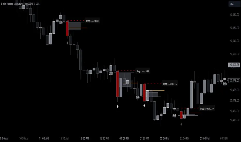
Bewakoof stock indicator**Title**: "Bewakoof Stock Indicator: Multi-Timeframe RSI and SuperTrend Entry-Exit System"
---
### Description
The **Bewakoof Stock Indicator** is an original trading tool that combines multi-timeframe RSI analysis with the SuperTrend indicator to create reliable entry and exit signals for trending markets. This indicator is designed for traders looking to follow strong trends with built-in risk management. By filtering entries through short- and long-term momentum and utilizing dynamic trailing exits, this indicator provides a structured approach to trading.
#### Indicator Components
1. **Multi-Timeframe RSI Analysis**:
- The Relative Strength Index (RSI) is calculated across three timeframes: Daily, Weekly, and Monthly.
- By examining multiple timeframes, the indicator confirms that trends align over short, medium, and long-term intervals, making buy signals more reliable.
- **Buy Condition**: All three RSI values must meet these thresholds:
- **Daily RSI > 50** – indicates short-term upward momentum,
- **Weekly RSI > 60** – signals medium-term strength,
- **Monthly RSI > 60** – confirms long-term trend alignment.
- This filtering process ensures that buy signals are generated only in stable, upward-trending markets.
2. **SuperTrend Confirmation**:
- The SuperTrend (20-period ATR with a multiplier of 2) acts as a trend filter and trailing stop mechanism.
- For a buy condition to be valid, the closing price must be above the SuperTrend level, verifying that the market is trending up.
- The combination of RSI and SuperTrend helps to avoid false signals, focusing only on well-established trends.
#### Trade Signals
- **Buy Signal**: When both the multi-timeframe RSI and SuperTrend conditions are met, a buy signal is triggered, indicated by a “BUY” label on the chart with details:
- **Entry Price**,
- **Initial Stop-Loss** (set at the SuperTrend level for risk control),
- **Target 1** – calculated with a 1:1 risk-reward ratio based on the initial stop-loss,
- **Target 2** – calculated with a 1:2 risk-reward ratio based on the initial stop-loss.
- **Exit Signals**: This indicator provides two exit strategies to protect profits:
1. **Fixed Stop-Loss**: Automatically set at the SuperTrend level at the time of entry to limit risk.
2. **Trailing Exit**: Exits are triggered if the price crosses below the SuperTrend level, adapting to potential trend reversals.
#### Labeling & Alerts
The **Bewakoof Stock Indicator** offers intuitive labeling and alert options:
- **Labels**: Buy and exit points are clearly marked, showing entry, stop-loss, and targets directly on the chart.
- **Alerts**: Custom alerts can be set for:
- **Buy signals** when both conditions are met, and
- **Exit signals** triggered by the stop-loss or trailing exit.
#### Use Case and Benefits
This indicator is ideal for trend-following traders who value risk control and trend confirmation:
- **Stronger Trend Signals**: By requiring RSI alignment across multiple timeframes, this indicator focuses only on trades with strong trend momentum.
- **Dynamic Risk Management**: Using both fixed and trailing exits enables flexible trade management, balancing risk and potential reward.
- **Simple Trade Execution**: The chart labels and alerts simplify trade decisions, making it easy to enter, manage, and exit trades.
#### How to Use
1. **Add** the Bewakoof Stock Indicator to your chart.
2. **Watch** for the "BUY" label as your entry point.
3. **Manage the trade** using the labeled stop-loss and target levels.
4. **Exit** on either a stop-loss hit or when the price crosses below the SuperTrend for a trailing exit.
The **Bewakoof Stock Indicator** is a complete solution for trend-following traders, combining the strength of multi-timeframe RSI with the SuperTrend’s trend-following capabilities. This systematic approach aims to provide high-confidence entries and effective risk management, empowering traders to follow trends with precision and control.
Moving Average Pullback Signals [UAlgo]The "Moving Average Pullback Signals " indicator is designed to identify potential trend continuation or reversal points based on moving average (MA) pullback patterns. This tool combines multiple types of moving averages, customized trend validation parameters, and candlestick wick patterns to provide reliable buy and sell signals. By leveraging several advanced MA methods (such as TEMA, DEMA, ZLSMA, and McGinley-D), this script can adapt to different market conditions, providing traders with flexibility and more precise trend-based entries and exits. The addition of a gradient color-coded moving average line and wick validation logic enables traders to visualize market sentiment and trend strength dynamically.
🔶 Key Features
Multiple Moving Average (MA) Calculation Methods: This indicator offers various MA calculation types, including SMA, EMA, DEMA, TEMA, ZLSMA, and McGinley-D, allowing traders to select the MA that best fits their strategy.
Trend Validation and Pattern Recognition: The indicator includes a customizable trend validation length, ensuring that the trend is consistent before buy/sell signals are generated. The "Trend Pattern Mode" setting provides flexibility between "No Trend in Progress," "Trend Continuation," and "Both," tailoring signals to the trader’s preferred style.
Wick Validation Logic: To enhance the accuracy of entries, this indicator identifies specific wick patterns for bullish or bearish pullbacks, which signal potential trend continuation or reversal. Wick length and validation factor are adjustable to suit various market conditions and timeframes.
Gradient Color-coded MA Line: This feature provides a quick visual cue for trend strength, with color changes reflecting relative highs and lows of the MA, enhancing market sentiment interpretation.
Alerts for Buy and Sell Signals: Alerts are triggered when either a bullish or bearish pullback is detected, allowing traders to receive instant notifications without continuously monitoring the chart.
Visual Labels for Reversal Points: The indicator plots labels ("R") at potential reversal points, with color-coded labels for bullish (green) and bearish (red) pullbacks, highlighting pullback opportunities that align with the trend or reversal potential.
🔶 Disclaimer
Use with Caution: This indicator is provided for educational and informational purposes only and should not be considered as financial advice. Users should exercise caution and perform their own analysis before making trading decisions based on the indicator's signals.
Not Financial Advice: The information provided by this indicator does not constitute financial advice, and the creator (UAlgo) shall not be held responsible for any trading losses incurred as a result of using this indicator.
Backtesting Recommended: Traders are encouraged to backtest the indicator thoroughly on historical data before using it in live trading to assess its performance and suitability for their trading strategies.
Risk Management: Trading involves inherent risks, and users should implement proper risk management strategies, including but not limited to stop-loss orders and position sizing, to mitigate potential losses.
No Guarantees: The accuracy and reliability of the indicator's signals cannot be guaranteed, as they are based on historical price data and past performance may not be indicative of future results.
Volumetric Rejection Blocks [UAlgo]The Volumetric Rejection Blocks is designed to help traders identify and visualize key price levels where volumetric rejections occur, which may indicate a shift in market sentiment. These rejections can signal potential trend reversals or areas where price action is likely to face support or resistance. By drawing rejection blocks based on volumetric strength, the indicator allows users to observe where significant buying or selling pressure has been exerted, which can be used as a reference point for future price action.
Also indicator dynamically calculates swing highs and lows, analyzes bullish and bearish strengths based on volume-weighted price movements, and displays rejection blocks on the chart. Each rejection block represents an area where the price attempted to move beyond a certain level but faced rejection, either on a close or wick basis. This can be particularly useful for traders who rely on market structure and order flow to make informed decisions about entering or exiting trades.
🔶 Key Features
Swing Length Customization: Allows users to define the swing length, helping tailor the sensitivity of the swing high and low detection to the specific market conditions.
Rejection Block Visualization: Displays up to the last 10 rejection blocks based on user settings, clearly marking areas of significant bullish or bearish rejections.
Volumetric Strength Analysis: The indicator calculates bullish and bearish strength for each rejection block, based on volume-weighted price movements over the last few bars, giving insight into the intensity of the rejection.
Violation Check Type: Offers two options for violation detection—"Close" and "Wick". This allows traders to specify whether a price level is considered broken only if it closes beyond the level or if any wick breaches it.
Bullish and Bearish Block Coloring: Rejection blocks are colored to represent bullish (green) and bearish (red) rejection areas. The color transparency can be adjusted for clear visibility overlaid on the price chart.
Market Structure Labels: Labels and lines marking "Market Structure Shift" (MSS) and "Break of Structure" (BOS) are displayed, giving traders context about significant market structure changes.
🔶 Interpreting the Indicator
Rejection Blocks: These colored blocks on the chart indicate areas where the price faced significant buying or selling pressure. A green block suggests a bullish rejection (support zone), where buyers absorbed the sell-off, potentially pushing the price upward. Conversely, a red block indicates a bearish rejection (resistance zone), where sellers overpowered buyers, potentially driving the price lower.
Strength Analysis: The width of the green and red sections within a rejection block represents the relative bullish and bearish strengths. A wider green section indicates stronger bullish support, while a wider red section suggests more robust bearish resistance. This helps traders gauge the likelihood of price holding or breaching these levels.
Market Structure Shift (MSS) and Break of Structure (BOS): The indicator automatically detects and labels significant changes in market structure. An "MSS" label indicates the first break, suggesting a potential shift in trend direction. A "BOS" label indicates a subsequent confirmation in trend direction, allowing traders to recognize potential trend continuations.
Violation Check: Traders can choose how to interpret breaks of these rejection blocks. Using the "Close" option provides a more conservative approach, requiring a close beyond the level for confirmation. The "Wick" option is more aggressive, treating any wick beyond the level as a break.
🔶 Disclaimer
Use with Caution: This indicator is provided for educational and informational purposes only and should not be considered as financial advice. Users should exercise caution and perform their own analysis before making trading decisions based on the indicator's signals.
Not Financial Advice: The information provided by this indicator does not constitute financial advice, and the creator (UAlgo) shall not be held responsible for any trading losses incurred as a result of using this indicator.
Backtesting Recommended: Traders are encouraged to backtest the indicator thoroughly on historical data before using it in live trading to assess its performance and suitability for their trading strategies.
Risk Management: Trading involves inherent risks, and users should implement proper risk management strategies, including but not limited to stop-loss orders and position sizing, to mitigate potential losses.
No Guarantees: The accuracy and reliability of the indicator's signals cannot be guaranteed, as they are based on historical price data and past performance may not be indicative of future results.

Target Trend [BigBeluga]The Target Trend indicator is a trend-following tool designed to assist traders in capturing directional moves while managing entry, stop loss, and profit targets visually on the chart. Using adaptive SMA bands as the core trend detection method, this indicator dynamically identifies shifts in trend direction and provides structured exit points through customizable target levels.
SP500:
🔵 IDEA
The Target Trend indicator’s concept is to simplify trade management by providing automated visual cues for entries, stops, and targets directly on the chart. When a trend change is detected, the indicator prints an up or down triangle to signal entry direction, plots three customizable target levels for potential exits, and calculates a stop-loss level below or above the entry point. The indicator continuously adapts as price moves, making it easier for traders to follow and manage trades in real time.
When price crosses a target level, the label changes to a check mark, confirming that the target has been achieved. Similarly, if the stop-loss level is hit, the label changes to an "X," and the line becomes dashed, indicating that the stop loss has been activated. This feature provides traders with a clear visual trail of whether their targets or stop loss have been hit, allowing for easier trade tracking and exit strategy management.
🔵 KEY FEATURES & USAGE
SMA Bands for Trend Detection: The indicator uses adaptive SMA bands to identify the trend direction. When price crosses above or below these bands, a new trend is detected, triggering entry signals. The entry point is marked on the chart with a triangle symbol, which updates with each new trend change.
Automated Targets and Stop Loss Management: Upon a new trend signal, the indicator automatically plots three price targets and a stop loss level. These levels provide traders with structured exit points for potential gains and a clear risk limit. The stop loss is placed below or above the entry point, depending on the trend direction, to manage downside risk effectively.
Visual Target and Stop Loss Validation: As price hits each target, the label beside the level updates to a check mark, indicating that the target has been reached. Similarly, if the stop loss is activated, the stop loss label changes to an "X," and the line becomes dashed. This feature visually confirms whether targets or stop losses are hit, simplifying trade management.
The indicator also marks the entry price at each trend change with a label on the chart, allowing traders to quickly see their initial entry point relative to current price and target levels.
🔵 CUSTOMIZATION
Trend Length: Set the lookback period for the trend-detection SMA bands to adjust the sensitivity to trend changes.
Targets Setting: Customize the number and spacing of the targets to fit your trading style and market conditions.
Visual Styles: Adjust the appearance of labels, lines, and symbols on the chart for a clearer view and personalized layout.
🔵 CONCLUSION
The Target Trend indicator offers a streamlined approach to trend trading by integrating entry, target, and stop loss management into a single visual tool. With automatic tracking of target levels and stop loss hits, it helps traders stay focused on the current trend while keeping track of risk and reward with minimal effort.
PTS - Bollinger Bands with Trailing StopPTS - Bollinger Bands with Trailing Stop Strategy
Overview
The "PTS - Bollinger Bands with Trailing Stop" strategy is designed to capitalize on strong bullish market movements by combining the Bollinger Bands indicator with a dynamic trailing stop based on the Average True Range (ATR). This strategy aims to enter long positions during upward breakouts and protect profits through an adaptive exit mechanism.
Key Features
1. Bollinger Bands Indicator
Basis Moving Average Type: Choose from SMA, EMA, SMMA, WMA, or VWMA for the Bollinger Bands' basis line. Length: Adjustable period for calculating the moving average and standard deviation (default is 20). Standard Deviation Multiplier (StdDev): Determines the width of the bands (default is 2.0). Source: Select the price data used for calculations (default is the closing price).
2. Entry Conditions
The strategy enters a long position when the closing price crosses above the upper Bollinger Band , indicating strong upward momentum.
3. Exit Conditions
Trailing Stop Loss: Implemented using ATR to adjust dynamically with market volatility. ATR Length: Period for calculating ATR (default is 14). ATR Multiplier for Trailing Stop: Determines how closely the trailing stop follows the price (default is 2.0). Close Below Lower Bollinger Band: The strategy exits the long position if the closing price crosses below the lower Bollinger Band .
4. Risk Management
Commission and Slippage: Commission is set at 0.1%; slippage is set to 3. Position Sizing: Uses 100% of equity per trade (adjustable).
5. Date Range Filter
Specify the time period during which the strategy is active. Start Date: January 1, 2018. End Date: December 31, 2069.
Customizable Inputs
BB Length: Adjust the period for Bollinger Bands calculation. BB StdDev: Modify the standard deviation multiplier. Basis MA Type: Select the moving average type. Source: Choose the price data source. Offset: Shift the Bollinger Bands on the chart. ATR Length: Set the period for ATR calculation. ATR Multiplier for Trailing Stop: Adjust the trailing stop sensitivity.
Thought for 1m 7s
Description for the "PTS - Bollinger Bands with Trailing Stop" Strategy
PTS - Bollinger Bands with Trailing Stop Strategy
Overview
The "PTS - Bollinger Bands with Trailing Stop" strategy is designed to capitalize on strong bullish market movements by combining the Bollinger Bands indicator with a dynamic trailing stop based on the Average True Range (ATR). This strategy aims to enter long positions during upward breakouts and protect profits through an adaptive exit mechanism.
Key Features
1. Bollinger Bands Indicator
Basis Moving Average Type: Choose from SMA, EMA, SMMA, WMA, or VWMA for the Bollinger Bands' basis line. Length: Adjustable period for calculating the moving average and standard deviation (default is 20). Standard Deviation Multiplier (StdDev): Determines the width of the bands (default is 2.0). Source: Select the price data used for calculations (default is the closing price).
2. Entry Conditions
The strategy enters a long position when the closing price crosses above the upper Bollinger Band , indicating strong upward momentum.
3. Exit Conditions
Trailing Stop Loss: Implemented using ATR to adjust dynamically with market volatility. ATR Length: Period for calculating ATR (default is 14). ATR Multiplier for Trailing Stop: Determines how closely the trailing stop follows the price (default is 2.0). Close Below Lower Bollinger Band: The strategy exits the long position if the closing price crosses below the lower Bollinger Band .
4. Risk Management
Commission and Slippage: Commission is set at 0.1%; slippage is set to 3. Position Sizing: Uses 100% of equity per trade (adjustable).
5. Date Range Filter
Specify the time period during which the strategy is active. Start Date: January 1, 2018. End Date: December 31, 2069.
Customizable Inputs
BB Length: Adjust the period for Bollinger Bands calculation. BB StdDev: Modify the standard deviation multiplier. Basis MA Type: Select the moving average type. Source: Choose the price data source. Offset: Shift the Bollinger Bands on the chart. ATR Length: Set the period for ATR calculation. ATR Multiplier for Trailing Stop: Adjust the trailing stop sensitivity.
How the Strategy Works
1. Initialization
Calculates Bollinger Bands and ATR based on selected parameters.
2. Entry Logic
Opens a long position when the closing price exceeds the upper Bollinger Band.
3. Exit Logic
Uses a trailing stop loss based on ATR. Exits if the closing price drops below the lower Bollinger Band.
4. Date Filtering
Executes trades only within the specified date range.
Advantages
Adaptive Risk Management: Trailing stop adjusts to market volatility. Simplicity: Clear entry and exit signals. Customizable Parameters: Tailor the strategy to different assets or conditions.
Considerations
Aggressive Position Sizing: Using 100% equity per trade is high-risk. Market Conditions: Best in trending markets; may produce false signals in sideways markets. Backtesting: Always test on historical data before live trading.
Disclaimer
This strategy is intended for educational and informational purposes only. Trading involves significant risk, and past performance is not indicative of future results. Assess your financial situation and consult a financial advisor if necessary.
Usage Instructions
1. Apply the Strategy: Add it to your TradingView chart. 2. Configure Inputs: Adjust parameters to suit your style and asset. 3. Analyze Backtest Results: Use the Strategy Tester. 4. Optimize Parameters: Experiment with input values. 5. Risk Management: Evaluate position sizing and incorporate risk controls.
Final Notes
The "PTS - Bollinger Bands with Trailing Stop" strategy provides a framework to leverage momentum breakouts while managing risk through adaptive trailing stops. Customize and test thoroughly to align with your trading objectives.
HBK Price Action Strategy HBKPrice Action Strategy for XAUUSD with a Favorable Risk-Reward Ratio
Understanding the Strategy:
This strategy leverages price action principles to identify potential entry and exit points for XAUUSD on a 5-minute timeframe. The core idea is to identify price action patterns that suggest a high probability of a particular direction, and then to set stop-loss and take-profit levels to manage risk and reward.
Key Price Action Patterns to Watch:
Pin Bar: A pin bar is a candlestick with a long wick in one direction and a small body in the opposite direction. It often signals a reversal in the current trend.
Inside Bar: An inside bar forms when the current candle's high is lower than the previous candle's high, and the current candle's low is higher than the previous candle's low. It often indicates indecision or a potential breakout.
Engulfing Pattern: An engulfing pattern occurs when the current candle completely engulfs the previous candle. A bullish engulfing pattern signals a potential uptrend, while a bearish engulfing pattern signals a potential downtrend.
Risk-Reward Ratio:
A favorable risk-reward ratio is crucial for long-term trading success. Aim for a minimum risk-reward ratio of 1:2, meaning you risk $1 to potentially gain $2.
Entry and Exit Signals:
Long Entry:
Identify a bullish pin bar or engulfing pattern.
Wait for a confirmation candle to close above the pin bar's high or the engulfing pattern's high.
Place a stop-loss below the recent swing low.
Set a take-profit target at a key resistance level or a multiple of the stop-loss distance.
Short Entry:
Identify a bearish pin bar or engulfing pattern.
Wait for a confirmation candle to close below the pin bar's low or the engulfing pattern's low.
Place a stop-loss above the recent swing high.
Set a take-profit target at a key support level or a multiple of the stop-loss distance.
Additional Tips:
Use Support and Resistance Levels: Identify key support and resistance levels to set your stop-loss and take-profit targets.
Consider Market Sentiment: Pay attention to market sentiment and news events that may impact gold prices.
Manage Risk: Always use stop-loss orders to limit potential losses.
Be Patient: Don't force trades. Wait for high-probability setups.
Practice Discipline: Stick to your trading plan and avoid impulsive decisions.
Remember:
Price action trading requires practice and patience.
Backtest your strategy on historical data to refine your approach.
Always adapt to changing market conditions.
By following these guidelines and practicing disciplined risk management, you can increase your chances of success in trading XAUUSD on a 5-minute timeframe.

Engulfing Pattern & Impulse [UAlgo]The Engulfing Pattern & Impulse is a tool designed for technical traders who utilize price action and volume analysis to assess market trends and potential reversals. This indicator identifies two powerful trading signals: Engulfing Patterns and Volume Impulses, which are essential components for evaluating potential bullish or bearish market momentum.
Engulfing Patterns are classic candlestick formations often associated with reversals or trend continuations, depending on the overall trend context. This indicator highlights both bullish and bearish engulfing patterns based on configurable criteria such as trend detection settings, comparison with average body size, and a customizable body multiplier for validation. The Volume Impulse feature signals moments of significant volume compared to historical levels, which often precede substantial price movements. Together, these features provide traders with a versatile tool for better timing entry and exit points.
The indicator also offers an adaptive trend detection system, allowing traders to choose from multiple methods (e.g., SMA50 or SMA50/SMA200 combinations) to assess the trend context, making it ideal for various market conditions.
🔶Key Features
Engulfing Pattern Detection: Identifies bullish and bearish engulfing patterns with customizable parameters, including body length and average size comparison.
Configurable trend basis: Choose between SMA50 or SMA50 with SMA200 to define trend direction.
Body size multiplier: Adjust the size threshold for valid engulfing patterns, providing flexibility based on market conditions.
Volume Impulse Signal: Highlights volume spikes that meet or exceed a specified multiplier, which can indicate increased buying or selling interest.
Customizable volume period and multiplier: Allows you to tailor the volume impulse detection based on the instrument’s average volume behavior.
Trend Detection Options: Select different trend detection methods to suit various trading styles and instruments.
SMA50-based detection: Classifies the trend based on the position of price relative to the 50-period SMA.
SMA50 and SMA200 combination: Incorporates a dual-moving average approach, classifying trends based on the relationship between price, SMA50, and SMA200.
Enhanced Visualization: Distinguishes bullish and bearish signals with customizable colors, providing clear and immediate visual cues for easy interpretation.
Custom label colors: Allows you to set distinct colors for bullish, bearish, and neutral signals for quick identification.
Pattern filtering: Enable or disable specific patterns (Bullish, Bearish, or Both) based on your trading preferences.
🔶 Interpreting Indicator
Bullish Engulfing Pattern: Indicates a potential bullish reversal in a downtrend. This signal occurs when a white candlestick with a body size exceeding a specified multiplier completely engulfs the previous black candlestick. The pattern will display a “BE” label below the candle if it meets the criteria, signaling potential upward momentum.
Bearish Engulfing Pattern: Indicates a potential bearish reversal in an uptrend. A black candlestick with a body size exceeding the specified multiplier fully engulfs the previous white candlestick, signaling possible downward movement. The “BE” label appears above the candle to denote this pattern.
Volume Impulse Up: Displays a “VI” label below the candle when the volume surpasses the defined multiplier, and the price closes higher than it opened, indicating strong upward buying interest.
Volume Impulse Down: Displays a “VI” label above the candle when the volume meets or exceeds the specified threshold, and the price closes lower than it opened, signaling strong selling pressure.
Indicator uses the SMA50 and SMA200 to determine trend direction due to their popularity in technical analysis as indicators of medium- and long-term trends. The SMA50 reflects the average price over the past 50 periods, providing insight into intermediate trends, while the SMA200 is often used to identify the broader trend direction. These SMAs help traders quickly assess whether the market is in an uptrend, downtrend, or consolidation phase, enhancing decision-making for both short-term and long-term strategies.
🔶 Disclaimer
Use with Caution: This indicator is provided for educational and informational purposes only and should not be considered as financial advice. Users should exercise caution and perform their own analysis before making trading decisions based on the indicator's signals.
Not Financial Advice: The information provided by this indicator does not constitute financial advice, and the creator (UAlgo) shall not be held responsible for any trading losses incurred as a result of using this indicator.
Backtesting Recommended: Traders are encouraged to backtest the indicator thoroughly on historical data before using it in live trading to assess its performance and suitability for their trading strategies.
Risk Management: Trading involves inherent risks, and users should implement proper risk management strategies, including but not limited to stop-loss orders and position sizing, to mitigate potential losses.
No Guarantees: The accuracy and reliability of the indicator's signals cannot be guaranteed, as they are based on historical price data and past performance may not be indicative of future results.

Multi Fibonacci Supertrend with Signals【FIbonacciFlux】Multi Fibonacci Supertrend with Signals (MFSS)
Overview
The Multi Fibonacci Supertrend with Signals (MFSS) is an advanced technical analysis tool that combines multiple Supertrend indicators using Fibonacci ratios to identify trend directions and potential trading opportunities.
Key Features
1. Fibonacci-Based Supertrend Levels
* Factor 1 (Weak) : 0.618 - The golden ratio
* Factor 2 (Medium) : 1.618 - The Fibonacci ratio
* Factor 3 (Strong) : 2.618 - The extension ratio
2. Visual Components
* Multi-layered Trend Lines
* Different line weights for easy identification
* Progressive transparency from Factor 1 to Factor 3
* Color-coded trend directions (Green for bullish, Red for bearish)
* Dynamic Fill Areas
* Gradient fills between price and trend lines
* Visual representation of trend strength
* Automatic color adjustment based on trend direction
* Signal Indicators
* Clear BUY/SELL labels on chart
* Position-adaptive signal placement
* High-visibility color scheme
3. Signal Generation Logic
The system generates signals based on two key conditions:
* Primary Condition :
* BUY : Price crossunder Supertrend2 (Factor 1.618)
* SELL : Price crossover Supertrend2 (Factor 1.618)
* Confirmation Filter :
* Signals only trigger when Supertrend3 confirms the trend direction
* Reduces false signals in volatile markets
Technical Details
Input Parameters
* ATR Period : 10 (default)
* Customizable for different market conditions
* Affects sensitivity of all Supertrend levels
* Factor Settings :
* All factors are customizable
* Default values based on Fibonacci sequence
* Minimum value: 0.01
* Step size: 0.01
Alert System
* Built-in alert conditions
* Customizable alert messages
* Real-time notification support
Use Cases
* Trend Trading
* Identify strong trend directions
* Filter out weak signals
* Confirm trend continuations
* Risk Management
* Multiple trend levels for stop-loss placement
* Clear entry and exit signals
* Trend strength visualization
* Market Analysis
* Multi-timeframe analysis capability
* Trend strength assessment
* Market structure identification
Benefits
* Reliability
* Based on proven Supertrend algorithm
* Enhanced with Fibonacci mathematics
* Multiple confirmation levels
* Clarity
* Clear visual signals
* Easy-to-interpret interface
* Reduced noise in signal generation
* Flexibility
* Customizable parameters
* Adaptable to different markets
* Suitable for various trading styles
Performance Considerations
* Optimized code structure
* Efficient calculation methods
* Minimal resource usage
Installation and Usage
Setup
* Add indicator to chart
* Adjust parameters if needed
* Enable alerts as required
Best Practices
* Use with other confirmation tools
* Adjust factors based on market volatility
* Consider timeframe appropriateness
Backtesting Results and Strategy Performance
This indicator is specifically designed for pullback trading with optimized risk-reward ratios in trend-following strategies. Below are the detailed backtesting results from our proprietary strategy implementation:
BTCUSDT Performance (Binance)
* Test Period: Approximately 7 years
* Risk-Reward Ratio: 2:1
* Take Profit: 8%
* Stop Loss: 4%
Key Metrics (BTCUSDT):
* Net Profit: +2,579%
* Total Trades: 551
* Win Rate: 44.8%
* Profit Factor: 1.278
* Maximum Drawdown: 42.86%
ETHUSD Performance (Binance)
* Risk-Reward Ratio: 4.33:1
* Take Profit: 13%
* Stop Loss: 3%
Key Metrics (ETHUSD):
* Net Profit: +8,563%
* Total Trades: 581
* Win Rate: 32%
* Profit Factor: 1.32
* Maximum Drawdown: 55%
Strategy Highlights:
* Optimized for pullback trading in strong trends
* Focus on high risk-reward ratios
* Proven effectiveness in major cryptocurrency pairs
* Consistent performance across different market conditions
* Robust profit factor despite moderate win rates
Note: These results are from our proprietary strategy implementation and should be used as reference only. Individual results may vary based on market conditions and implementation.
Important Considerations:
* The strategy demonstrates strong profitability despite lower win rates, emphasizing the importance of proper risk-reward ratios
* Higher drawdowns are compensated by significant overall returns
* The system shows adaptability across different cryptocurrencies with consistent profit factors
* Results suggest optimal performance in volatile crypto markets
Real Trading Examples
BTCUSDT 4-Hour Chart Analysis
Example of pullback strategy implementation on Bitcoin, showing clear trend definition and entry points
ETHUSDT 4-Hour Chart Analysis
Ethereum chart demonstrating effective signal generation during strong trends
BTCUSDT Detailed Signal Example (15-Minute Scalping)
Close-up view of signal generation and trend confirmation process on 15-minute timeframe, demonstrating the indicator's effectiveness for scalping operations
Chart Analysis Notes:
* Green and red zones clearly indicate trend direction
* Multiple timeframe confirmation visible through different Supertrend levels
* Clear entry signals during pullbacks in established trends
* Precise stop-loss placement opportunities below support levels
Implementation Guidelines:
* Wait for main trend confirmation from Factor 3 (2.618)
* Enter trades on pullbacks to Factor 2 (1.618)
* Use Factor 1 (0.618) for fine-tuning entry points
* Place stops below the relevant Supertrend level
Footnotes:
* Charts provided are from Binance exchange, using both 4-hour and 15-minute timeframes
* Trading view screenshots captured during actual market conditions
* Indicators shown: Multi Fibonacci Supertrend with all three factors
* Time period: Recent market activity showing various market conditions
Important Notice:
These charts are for educational purposes only. Past performance does not guarantee future results. Always conduct your own analysis and risk management.
Disclaimer
This indicator is for informational purposes only. Past performance is not indicative of future results. Always conduct proper risk management and due diligence.
License
Open source under MIT License
Author's Note
Contributions and suggestions for improvement are welcome. Please feel free to fork and enhance.
