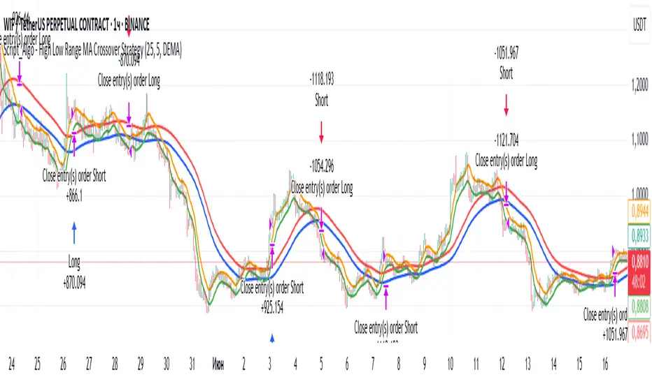
Script_Algo - High Low Range MA Crossover Strategy🎯 Core Concept
This strategy uses modified moving averages crossover, built on maximum and minimum prices, to determine entry and exit points in the market. A key advantage of this strategy is that it avoids most false signals in trendless conditions, which is characteristic of traditional moving average crossover strategies. This makes it possible to improve the risk/reward ratio and, consequently, the strategy's profitability.
📊 How the Strategy Works
Main Mechanism
The strategy builds 4 moving averages:
Two senior MAs (on high and low) with a longer period
Two junior MAs (on high and low) with a shorter period
Buy signal 🟢: when the junior MA of lows crosses above the senior MA of highs
Sell signal 🔴: when the junior MA of highs crosses below the senior MA of lows
As seen on the chart, it was potentially possible to make 9X on the WIFUSDT cryptocurrency pair in just a year and a half. However, be careful—such results may not necessarily be repeated in the future.
Special Feature
Position closing priority ❗: if an opposite signal arrives while a position is open, the strategy first closes the current position and only then opens a new one
⚙️ Indicator Settings
Available Moving Average Types
EMA - Exponential MA
SMA - Simple MA
SSMA - Smoothed MA
WMA - Weighted MA
VWMA - Volume Weighted MA
RMA - Adaptive MA
DEMA - Double EMA
TEMA - Triple EMA
Adjustable Parameters
Senior MA Length - period for long-term moving averages
Junior MA Length - period for short-term moving averages
✅ Advantages of the Strategy
🛡️ False Signal Protection - using two pairs of modified MAs reduces the number of false entries
🔄 Configuration Flexibility - ability to choose MA type and calculation periods
⚡ Automatic Switching - the strategy automatically closes the current position when receiving an opposite signal
📈 Visual Clarity - all MAs are displayed on the chart in different colors
⚠️ Disadvantages and Risks
📉 Signal Lag - like all MA-based strategies, it may provide delayed signals during sharp movements
🔁 Frequent Switching - in sideways markets, it may lead to multiple consecutive position openings/closings
📊 Requires Optimization - optimal parameters need to be selected for different instruments and timeframes
💡 Usage Recommendations
Backtest - test the strategy's performance on historical data
Optimize Parameters - select MA periods suitable for the specific trading instrument
Use Filters - add additional filters to confirm signals
Manage Risks - always use stop-loss and take-profit orders.
You can safely connect to the exchange via webhook and enjoy trading.
Good luck and profits to everyone!!
Cerca negli script per "the strat"
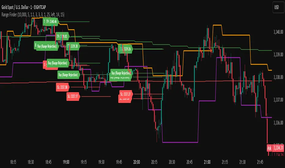
Range FinderRange Finder Strategy for TradingView
Overview
The Range Finder Strategy is a sophisticated trading system designed for forex and cryptocurrency markets, leveraging dynamic range detection, wick-based rejection patterns, and EMA confluence to execute high-probability trades. This strategy identifies key price ranges using pivot points and triggers trades when price rejects from these boundaries with significant wick formations, aligning with the broader market trend as confirmed by EMA crossovers. It incorporates robust risk management, customizable parameters, and visual aids for clear trade visualization, making it suitable for both manual and automated trading on platforms like Bitget via webhook alerts.
Strategy Components
1. Dynamic Range Detection
Pivot Points: The strategy identifies range boundaries using pivot highs and lows, calculated with a user-defined Pivot Length (default: 5 bars left/right). These pivots mark significant swing points, defining the upper (range high) and lower (range low) boundaries of the price range.
Visualization: The range high is plotted as an orange line, and the range low as a purple line, using a broken line style (plot.style_linebr) to show only confirmed pivot levels, providing a clear visual of the trading range.
2. Wick-Based Rejection Pattern
Wick Detection: The strategy looks for rejection candles at the range boundaries, characterized by significant wicks. A wick is considered valid if its size is at least the user-defined Wick to Body Ratio (default: 1.1, or 10% larger than the candle body).
Sell Signal: Triggered when the high exceeds the range high, the candle closes bearish (close < open), and the upper wick meets the ratio requirement.
Buy Signal: Triggered when the low falls below the range low, the candle closes bullish (close > open), and the lower wick meets the ratio requirement.
Purpose: These wicks indicate strong rejection at key levels, often signaling a reversal back into the range, providing high-probability entry points.
3. EMA Trend Confirmation
EMA Calculation: Uses two Exponential Moving Averages (EMAs) calculated on a user-selectable timeframe (default: 5-minute):
EMA 200: Long-term trend indicator (plotted in red).
EMA 50: Short-term trend indicator (plotted in green).
Crossover Logic:
A bullish trend is confirmed when the EMA 50 crosses above the EMA 200 (ema_trend_up = true).
A bearish trend is confirmed when the EMA 50 crosses below the EMA 200 (ema_trend_down = true).
Confluence Requirement: Trades are only executed when the wick rejection aligns with the EMA trend (e.g., sell signals require close < ema200 and bearish trend; buy signals require close > ema200 and bullish trend).
4. Risk Management
Position Sizing: Calculated based on the user-defined Account Balance (default: $10,000) and Risk Per Trade (default: 2%). The position size is determined as risk_amount / stop_distance, where stop_distance is derived from the Average True Range (ATR, default period: 14).
Stop Loss (SL): Set using an ATR-based multiplier (SL Multiplier, default: 9.0). For sells, SL is placed above the high; for buys, below the low.
Take Profit (TP): Set using an ATR-based multiplier (TP Multiplier, default: 6.0) scaled by the Risk:Reward Ratio (default: 6.0), ensuring a favorable reward-to-risk profile.
Example: For a $10,000 account with 2% risk, if ATR is 0.5, the position size is 400 units, with SL and TP dynamically adjusted to market volatility.
5. Trade Execution
Sell Entry: Triggered on a wick rejection above the range high, with bearish EMA confluence (ema_trend_down and close < ema200). Enters a short position with calculated SL and TP.
Buy Entry: Triggered on a wick rejection below the range low, with bullish EMA confluence (ema_trend_up and close > ema200). Enters a long position with calculated SL and TP.
Exit Logic: Uses strategy.exit to set SL and TP levels, closing trades when either is hit.
6. Visual Feedback
Lines and Labels: Upon trade entry, the strategy plots:
Red SL line and label (e.g., "SL: 123.45").
Green TP line and label (e.g., "TP: 120.00").
Entry line (red for sell, green for buy) labeled with "Sell (Range Rejection)" or "Buy (Range Rejection)".
Customization: Users can adjust the Line Length (default: 25 bars) for how long lines persist and Label Position (left or right) for optimal chart visibility.
7. Alert Conditions
Webhook Integration: Generates alerts for Bitget webhook integration, providing JSON-formatted messages with trade details (action, contracts, market position, size, price, symbol, and timestamp).
Usage: Traders can set up automated trading by connecting these alerts to trading bots or platforms supporting webhooks.
Pivot Distance Strategy# Multi-Timeframe Pivot Distance Strategy
## Core Innovation & Originality
This strategy revolutionizes moving average crossover trading by applying MA logic to **pivot distance relationships** instead of raw price data. Unlike traditional MA crossovers that react to price changes, this system reacts to **structural momentum changes** in how current price relates to recent significant pivot levels, creating earlier signals with fewer false positives.
## Methodology & Mathematical Foundation
### Pivot Distance Oscillator
The strategy calculates:
- **High Pivot Percentage**: (Current Close / Last Pivot High) × 100
- **Low Pivot Percentage**: (Last Pivot Low / Current Close) × 100
- **Pivot Distance**: High Pivot Percentage - Low Pivot Percentage
This creates a standardized oscillator measuring market structure compression/expansion regardless of asset price or volatility.
### Multi-Timeframe Filter
Higher timeframe analysis provides directional bias:
- **HTF Long** → Allow long entries, force short exits
- **HTF Short** → Allow short entries, force long exits
- **HTF Squeeze** → Block all entries, force all exits
## Signal Generation Methods
### Method 1: Dual MA Crossover (Primary/Default)
**Fast MA (14 EMA)** and **Slow MA (50 SMA)** applied to pivot distance values:
- **Long Signal**: Fast MA crosses above Slow MA (accelerating bullish pivot momentum)
- **Short Signal**: Fast MA crosses below Slow MA (accelerating bearish pivot momentum)
**Key Advantage**:
- Traditional: Fast MA(price) crosses Slow MA(price) - reacts to price changes
- This Strategy: Fast MA(pivot distance) crosses Slow MA(pivot distance) - reacts to structural changes
- Result: Earlier signals, better trend identification, fewer ranging market whipsaws
### Method 2: MA Cross Zero
- **Long**: Pivot Distance MA crosses above zero
- **Short**: Pivot Distance MA crosses below zero
### Method 3: Pivot Distance Breakout (Squeeze-Based)
Uses dynamic threshold envelopes to detect compression/expansion cycles:
- **Long**: Distance breaks above dynamic breakout threshold after squeeze
- **Short**: Distance breaks below negative breakout threshold after squeeze
**Note**: Only the Breakout method uses threshold envelopes; MA Cross modes operate without them for cleaner signals.
## Risk Management Integration
- **ATR-Based Stops**: Entry ± (ATR × Multiplier) for stops/targets
- **Trailing Stops**: Dynamic adjustment based on profit thresholds
- **Cooldown System**: Prevents overtrading after stop-loss exits
## How to Use
### Setup (Default: MA Cross MA)
1. **Strategy Logic**: "MA Cross MA" for structural momentum signals
2. **MA Settings**: 14 EMA (fast) / 50 SMA (slow) - both adjustable
3. **Multi-Timeframe**: Enable HTF for trend alignment
4. **Risk Management**: ATR stop loss, ATR take profit
### Signal Interpretation
- **Blue/Purple lines**: Fast/Slow MAs of pivot distance
- **Green/Red histogram**: Positive/negative pivot distance
- **Triangle markers**: MA crossover entry signals
- **HTF display**: Shows higher timeframe bias (top-left)
### Trade Management
- **Entry**: Clean MA crossover with HTF alignment
- **Exit**: Opposite crossover, HTF change, or risk management triggers
## Unique Advantages
1. **Structural vs Price Momentum**: Captures market structure changes rather than just price movement, naturally filtering noise
2. **Multi-Modal Flexibility**: Three signal methods for different market conditions or strategies
3. **Timeframe Alignment**: HTF filtering improves win rates by preventing counter-trend trades

The Barking Rat LiteMomentum & FVG Reversion Strategy
The Barking Rat Lite is a disciplined, short-term mean-reversion strategy that combines RSI momentum filtering, EMA bands, and Fair Value Gap (FVG) detection to identify short-term reversal points. Designed for practical use on volatile markets, it focuses on precise entries and ATR-based take profit management to balance opportunity and risk.
Core Concept
This strategy seeks potential reversals when short-term price action shows exhaustion outside an EMA band, confirmed by momentum and FVG signals:
EMA Bands:
Parameters used: A 20-period EMA (fast) and 100-period EMA (slow).
Why chosen:
- The 20 EMA is sensitive to short-term moves and reflects immediate momentum.
- The 100 EMA provides a slower, structural anchor.
When price trades outside both bands, it often signals overextension relative to both short-term and medium-term trends.
Application in strategy:
- Long entries are only considered when price dips below both EMAs, identifying potential undervaluation.
- Short entries are only considered when price rises above both EMAs, identifying potential overvaluation.
This dual-band filter avoids counter-trend signals that would occur if only a single EMA was used, making entries more selective..
Fair Value Gap Detection (FVG):
Parameters used: The script checks for dislocations using a 12-bar lookback (i.e. comparing current highs/lows with values 12 candles back).
Why chosen:
- A 12-bar displacement highlights significant inefficiencies in price structure while filtering out micro-gaps that appear every few bars in high-volatility markets.
- By aligning FVG signals with candle direction (bullish = close > open, bearish = close < open), the strategy avoids random gaps and instead targets ones that suggest exhaustion.
Application in strategy:
- Bullish FVGs form when earlier lows sit above current highs, hinting at downward over-extension.
- Bearish FVGs form when earlier highs sit below current lows, hinting at upward over-extension.
This gives the strategy a structural filter beyond simple oscillators, ensuring signals have price-dislocation context.
RSI Momentum Filter:
Parameters used: 14-period RSI with thresholds of 80 (overbought) and 20 (oversold).
Why chosen:
- RSI(14) is a widely recognized momentum measure that balances responsiveness with stability.
- The thresholds are intentionally extreme (80/20 vs. the more common 70/30), so the strategy only engages at genuine exhaustion points rather than frequent minor corrections.
Application in strategy:
- Longs trigger when RSI < 20, suggesting oversold exhaustion.
- Shorts trigger when RSI > 80, suggesting overbought exhaustion.
This ensures entries are not just technically valid but also backed by momentum extremes, raising conviction.
ATR-Based Take Profit:
Parameters used: 14-period ATR, with a default multiplier of 4.
Why chosen:
- ATR(14) reflects the prevailing volatility environment without reacting too much to outliers.
- A multiplier of 4 is a pragmatic compromise: wide enough to let trades breathe in volatile conditions, but tight enough to enforce disciplined exits before mean reversion fades.
Application in strategy:
- At entry, a fixed target is set = Entry Price ± (ATR × 4).
- This target scales automatically with volatility: narrower in calm periods, wider in explosive markets.
By avoiding discretionary exits, the system maintains rule-based discipline.
Visual Signals on Chart
Blue “▲” below candle: Potential long entry
Orange/Yellow “▼” above candle: Potential short entry
Green “✔️”: Trade closed at ATR take profit
Blue (20 EMA) & Orange (100 EMA) lines: Dynamic channel reference
⚙️Strategy report properties
Position size: 25% equity per trade
Initial capital: 10,000.00 USDT
Pyramiding: 10 entries per direction
Slippage: 2 ticks
Commission: 0.055% per side
Backtest timeframe: 1-minute
Backtest instrument: HYPEUSDT
Backtesting range: Jul 28, 2025 — Aug 17, 2025
Note on Sample Size:
You’ll notice the report displays fewer than the ideal 100 trades in the strategy report above. This is intentional. The goal of the script is to isolate high-quality, short-term reversal opportunities while filtering out low-conviction setups. This means that the Barking Rat Lite strategy is very selective, filtering out over 90% of market noise. The brief timeframe shown in the strategy report here illustrates its filtering logic over a short window — not its full capabilities. As a result, even on lower timeframes like the 1-minute chart, signals are deliberately sparse — each one must pass all criteria before triggering.
For a larger dataset:
Once the strategy is applied to your chart, users are encouraged to expand the lookback range or apply the strategy to other volatile pairs to view a full sample.
💡Why 25% Equity Per Trade?
While it's always best to size positions based on personal risk tolerance, we defaulted to 25% equity per trade in the backtesting data — and here’s why:
Backtests using this sizing show manageable drawdowns even under volatile periods.
The strategy generates a sizeable number of trades, reducing reliance on a single outcome.
Combined with conservative filters, the 25% setting offers a balance between aggression and control.
Users are strongly encouraged to customize this to suit their risk profile.
What makes Barking Rat Lite valuable
Combines multiple layers of confirmation: EMA bands + FVG + RSI
Adaptive to volatility: ATR-based exits scale with market conditions
Clear, actionable visuals: Easy to monitor and manage trades

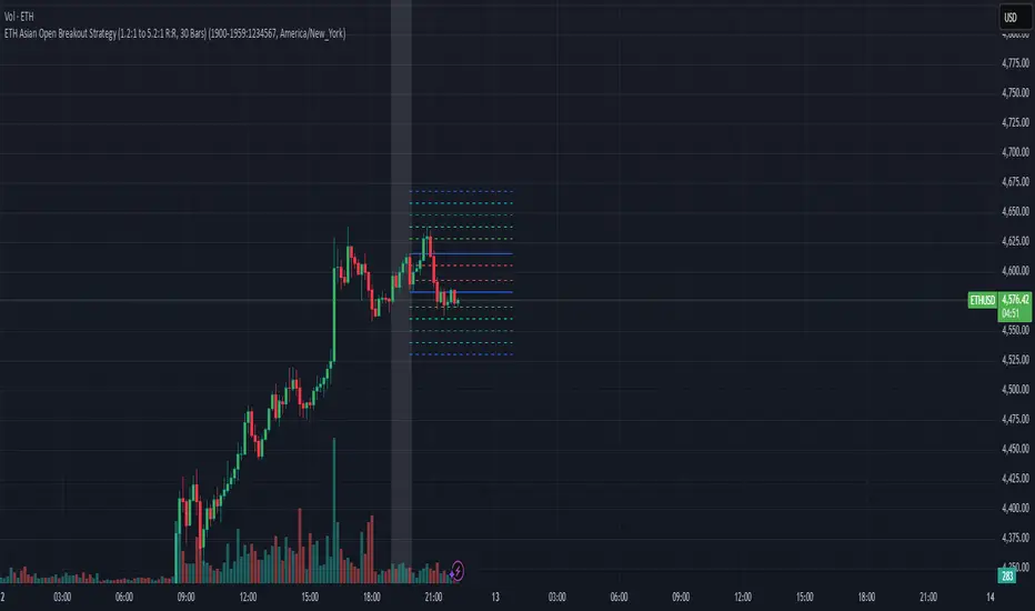
EAOBS by MIGVersion 1
1. Strategy Overview Objective: Capitalize on breakout movements in Ethereum (ETH) price after the Asian open pre-market session (7:00 PM–7:59 PM EST) by identifying high and low prices during the session and trading breakouts above the high or below the low.
Timeframe: Any (script is timeframe-agnostic, but align with session timing).
Session: Pre-market session (7:00 PM–7:59 PM EST, adjustable for other time zones, e.g., 12:00 AM–12:59 AM GMT).
Risk-Reward Ratios (R:R): Targets range from 1.2:1 to 5.2:1, with a fixed stop loss.
Instrument: Ethereum (ETH/USD or ETH-based pairs).
2. Market Setup Session Monitoring: Monitor ETH price action during the pre-market session (7:00 PM–7:59 PM EST), which aligns with the Asian market open (e.g., 9:00 AM–9:59 AM JST).
The script tracks the highest high and lowest low during this session.
Breakout Triggers: Buy Signal: Price breaks above the session’s high after the session ends (7:59 PM EST).
Sell Signal: Price breaks below the session’s low after the session ends.
Visualization: The session is highlighted on the chart with a white background.
Horizontal lines are drawn at the session’s high and low, extended for 30 bars, along with take-profit (TP) and stop-loss (SL) levels.
3. Entry Rules Long (Buy) Entry: Enter a long position when the price breaks above the session’s high price after 7:59 PM EST.
Entry price: Just above the session high (e.g., add a small buffer, like 0.1–0.5%, to avoid false breakouts, depending on volatility).
Short (Sell) Entry: Enter a short position when the price breaks below the session’s low price after 7:59 PM EST.
Entry price: Just below the session low (e.g., subtract a small buffer, like 0.1–0.5%).
Confirmation: Use a candlestick close above/below the breakout level to confirm the entry.
Optionally, add volume confirmation or a momentum indicator (e.g., RSI or MACD) to filter out weak breakouts.
Position Size: Calculate position size based on risk tolerance (e.g., 1–2% of account per trade).
Risk is determined by the stop-loss distance (10 points, as defined in the script).
4. Exit Rules Take-Profit Levels (in points, based on script inputs):TP1: 12 points (1.2:1 R:R).
TP2: 22 points (2.2:1 R:R).
TP3: 32 points (3.2:1 R:R).
TP4: 42 points (4.2:1 R:R).
TP5: 52 points (5.2:1 R:R).
Example for Long: If session high is 3000, TP levels are 3012, 3022, 3032, 3042, 3052.
Example for Short: If session low is 2950, TP levels are 2938, 2928, 2918, 2908, 2898.
Strategy: Scale out of the position (e.g., close 20% at TP1, 20% at TP2, etc.) or take full profit at a preferred TP level based on market conditions.
Stop-Loss: Fixed at 10 points from the entry.
Long SL: Session high - 10 points (e.g., entry at 3000, SL at 2990).
Short SL: Session low + 10 points (e.g., entry at 2950, SL at 2960).
Trailing Stop (Optional):After reaching TP2 or TP3, consider trailing the stop to lock in profits (e.g., trail by 10–15 points below the current price).
5. Risk Management per Trade: Limit risk to 1–2% of your trading account per trade.
Calculate position size: Account Size × Risk % ÷ (Stop-Loss Distance × ETH Price per Point).
Example: $10,000 account, 1% risk = $100. If SL = 10 points and 1 point = $1, position size = $100 ÷ 10 = 0.1 ETH.
Daily Risk Limit: Cap daily losses at 3–5% of the account to avoid overtrading.
Maximum Exposure: Avoid taking both long and short positions simultaneously unless using separate accounts or strategies.
Volatility Consideration: Adjust position size during high-volatility periods (e.g., major news events like Ethereum upgrades or macroeconomic announcements).
6. Trade Management Monitoring :Watch for breakouts after 7:59 PM EST.
Monitor price action near TP and SL levels using alerts or manual checks.
Trade Duration: Breakout lines extend for 30 bars (script parameter). Close trades if no TP or SL is hit within this period, or reassess based on market conditions.
Adjustments: If the market shows strong momentum, consider holding beyond TP5 with a trailing stop.
If the breakout fails (e.g., price reverses before TP1), exit early to minimize losses.
7. Additional Considerations Market Conditions: The 7:00 PM–7:59 PM EST session aligns with the Asian market open (e.g., Tokyo Stock Exchange open at 9:00 AM JST), which may introduce higher volatility due to Asian trading activity.
Avoid trading during low-liquidity periods or extreme volatility (e.g., major crypto news).
Check for upcoming events (e.g., Ethereum network upgrades, ETF decisions) that could impact price.
Backtesting: Test the strategy on historical ETH data using the session high/low breakouts for the 7:00 PM–7:59 PM EST window to validate performance.
Adjust TP/SL levels based on backtest results if needed.
Broker and Fees: Use a low-fee crypto exchange (e.g., Binance, Kraken, Coinbase Pro) to maximize R:R.
Account for trading fees and slippage in your position sizing.
Time zone Adjustment: Adjust session time input for your time zone (e.g., "0000-0059" for GMT).
Ensure your trading platform’s clock aligns with the script’s time zone (default: America/New_York).
8. Example Trade Scenario: Session (7:00 PM–7:59 PM EST) records a high of 3050 and a low of 3000.
Long Trade: Entry: Price breaks above 3050 (e.g., enter at 3051).
TP Levels: 3063 (TP1), 3073 (TP2), 3083 (TP3), 3093 (TP4), 3103 (TP5).
SL: 3040 (3050 - 10).
Position Size: For a $10,000 account, 1% risk = $100. SL = 11 points ($11). Size = $100 ÷ 11 = ~0.09 ETH.
Short Trade: Entry: Price breaks below 3000 (e.g., enter at 2999).
TP Levels: 2987 (TP1), 2977 (TP2), 2967 (TP3), 2957 (TP4), 2947 (TP5).
SL: 3010 (3000 + 10).
Position Size: Same as above, ~0.09 ETH.
Execution: Set alerts for breakouts, enter with limit orders, and monitor TPs/SL.
9. Tools and Setup Platform: Use TradingView to implement the Pine Script and visualize breakout levels.
Alerts: Set price alerts for breakouts above the session high or below the session low after 7:59 PM EST.
Set alerts for TP and SL levels.
Chart Settings: Use a 1-minute or 5-minute chart for precise session tracking.
Overlay the script to see high/low lines, TP levels, and SL levels.
Optional Indicators: Add RSI (e.g., avoid overbought/oversold breakouts) or volume to confirm breakouts.
10. Risk Warnings Crypto Volatility: ETH is highly volatile; unexpected news can cause rapid price swings.
False Breakouts: Breakouts may fail, especially in low-volume sessions. Use confirmation signals.
Leverage: Avoid high leverage (e.g., >5x) to prevent liquidation during volatile moves.
Session Accuracy: Ensure correct session timing for your time zone to avoid misaligned entries.
11. Performance Tracking Journaling :Record each trade’s entry, exit, R:R, and outcome.
Note market conditions (e.g., trending, ranging, news-driven).
Review: Weekly: Assess win rate, average R:R, and adherence to the plan.
Monthly: Adjust TP/SL or session timing based on performance.
MSTY-WNTR Rebalancing SignalMSTY-WNTR Rebalancing Signal
## Overview
The **MSTY-WNTR Rebalancing Signal** is a custom TradingView indicator designed to help investors dynamically allocate between two YieldMax ETFs: **MSTY** (YieldMax MSTR Option Income Strategy ETF) and **WNTR** (YieldMax Short MSTR Option Income Strategy ETF). These ETFs are tied to MicroStrategy (MSTR) stock, which is heavily influenced by Bitcoin's price due to MSTR's significant Bitcoin holdings.
MSTY benefits from upward movements in MSTR (and thus Bitcoin) through a covered call strategy that generates income but caps upside potential. WNTR, on the other hand, provides inverse exposure, profiting from MSTR declines but losing in rallies. This indicator uses Bitcoin's momentum and MSTR's relative strength to signal when to hold MSTY (bullish phases), WNTR (bearish phases), or stay neutral, aiming to optimize returns by switching allocations at key turning points.
Inspired by strategies discussed in crypto communities (e.g., X posts analyzing MSTR-linked ETFs), this indicator promotes an active rebalancing approach over a "set and forget" buy-and-hold strategy. In simulated backtests over the past 12 months (as of August 4, 2025), the optimized version has shown potential to outperform holding 100% MSTY or 100% WNTR alone, with an illustrative APY of ~125% vs. ~6% for MSTY and ~-15% for WNTR in one scenario.
**Important Disclaimer**: This is not financial advice. Past performance does not guarantee future results. Always consult a financial advisor. Trading involves risk, and you could lose money. The indicator is for educational and informational purposes only.
## Key Features
- **Momentum-Based Signals**: Uses a Simple Moving Average (SMA) on Bitcoin's price to detect bullish (price > SMA) or bearish (price < SMA) trends.
- **RSI Confirmation**: Incorporates MSTR's Relative Strength Index (RSI) to filter signals, avoiding overbought conditions for MSTY and oversold for WNTR.
- **Visual Cues**:
- Green upward triangle for "Hold MSTY".
- Red downward triangle for "Hold WNTR".
- Yellow cross for "Switch" signals.
- Background color: Green for MSTY, red for WNTR.
- **Information Panel**: A table in the top-right corner displays real-time data: BTC Price, SMA value, MSTR RSI, and current Allocation (MSTY, WNTR, or Neutral).
- **Alerts**: Configurable alerts for holding MSTY, holding WNTR, or switching.
- **Optimized Parameters**: Defaults are tuned (SMA: 10 days, RSI: 15 periods, Overbought: 80, Oversold: 20) based on simulations to reduce whipsaws and capture trends effectively.
## How It Works
The indicator's logic is straightforward yet effective for volatile assets like Bitcoin and MSTR:
1. **Primary Trigger (Bitcoin Momentum)**:
- Calculate the SMA of Bitcoin's closing price (default: 10-day).
- Bullish: Current BTC price > SMA → Potential MSTY hold.
- Bearish: Current BTC price < SMA → Potential WNTR hold.
2. **Secondary Filter (MSTR RSI Confirmation)**:
- Compute RSI on MSTR stock (default: 15-period).
- For bullish signals: If RSI > Overbought (80), signal Neutral (avoid overextended rallies).
- For bearish signals: If RSI < Oversold (20), signal Neutral (avoid capitulation bottoms).
3. **Allocation Rules**:
- Hold 100% MSTY if bullish and not overbought.
- Hold 100% WNTR if bearish and not oversold.
- Neutral otherwise (e.g., during choppy or extreme markets) – consider holding cash or avoiding trades.
4. **Rebalancing**:
- Switch signals trigger when the hold changes (e.g., from MSTY to WNTR).
- Recommended frequency: Weekly reviews or on 5% BTC moves to minimize trading costs (aim for 4-6 trades/year).
This approach leverages Bitcoin's influence on MSTR while mitigating the risks of MSTY's covered call drag during downtrends and WNTR's losses in uptrends.
## Setup and Usage
1. **Chart Requirements**:
- Apply this indicator to a Bitcoin chart (e.g., BTCUSD on Binance or Coinbase, daily timeframe recommended).
- Ensure MSTR stock data is accessible (TradingView supports it natively).
2. **Adding to TradingView**:
- Open the Pine Editor.
- Paste the script code.
- Save and add to your chart.
- Customize inputs if needed (e.g., adjust SMA/RSI lengths for different timeframes).
3. **Interpretation**:
- **Green Background/Triangle**: Allocate 100% to MSTY – Bitcoin is in an uptrend, MSTR not overbought.
- **Red Background/Triangle**: Allocate 100% to WNTR – Bitcoin in downtrend, MSTR not oversold.
- **Yellow Switch Cross**: Rebalance your portfolio immediately.
- **Neutral (No Signal)**: Panel shows "Neutral" – Hold cash or previous position; reassess weekly.
- Monitor the panel for key metrics to validate signals manually.
4. **Backtesting and Strategy Integration**:
- Convert to a strategy script by changing `indicator()` to `strategy()` and adding entry/exit logic for automated testing.
- In simulations (e.g., using Python or TradingView's backtester), it has outperformed buy-and-hold in volatile markets by ~100-200% relative APY, but results vary.
- Factor in fees: ETF expense ratios (~0.99%), trading commissions (~$0.40/trade), and slippage.
5. **Risk Management**:
- Use with a diversified portfolio; never allocate more than you can afford to lose.
- Add stop-losses (e.g., 10% trailing) to protect against extreme moves.
- Rebalance sparingly to avoid over-trading in sideways markets.
- Dividends: Reinvest MSTY/WNTR payouts into the current hold for compounding.
## Performance Insights (Simulated as of August 4, 2025)
Based on synthetic backtests modeling the last 12 months:
- **Optimized Strategy APY**: ~125% (by timing switches effectively).
- **Hold 100% MSTY APY**: ~6% (gains from BTC rallies offset by downtrends).
- **Hold 100% WNTR APY**: ~-15% (losses in bull phases outweigh bear gains).
In one scenario with stronger volatility, the strategy achieved ~4533% APY vs. 10% for MSTY and -34% for WNTR, highlighting its potential in dynamic markets. However, these are illustrative; real results depend on actual BTC/MSTR movements. Test thoroughly on historical data.
## Limitations and Considerations
- **Data Dependency**: Relies on accurate BTC and MSTR data; delays or gaps can affect signals.
- **Market Risks**: Bitcoin's volatility can lead to false signals (whipsaws); the RSI filter helps but isn't perfect.
- **No Guarantees**: This indicator doesn't predict the future. MSTR's correlation to BTC may change (e.g., due to regulatory events).
- **Not for All Users**: Best for intermediate/advanced traders familiar with ETFs and crypto. Beginners should paper trade first.
- **Updates**: As of August 4, 2025, this is version 1.0. Future updates may include volume filters or EMA options.
If you find this indicator useful, consider leaving a like or comment on TradingView. Feedback welcome for improvements!

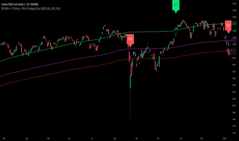
200 SMA (5%/-3% Buffer) for SPY & QQQ In my testing TQQQ is an absolute monster of an ETF that performs extremely well even from a buy and hold standpoint over long periods of time, its largest drawback is the massive drawdown exposure that it faces which can be easily sidestepped with this strategy.
This strategy is meant to basically abuse TQQQ's insane outperformance while augmenting the typical 200SMA strategy in a way that uses all of its strengths while avoiding getting whipsawed in sideways markets.
The strategy BUYS when price crosses 5% over the 200SMA and then SELLS when price drops 3% below the 200SMA. Between trades I'll be parking my entire account in SGOV.
So maximizing profit while minimizing risk.
You use the strategy based off of QQQ and then make the trades on TQQQ when it tells you to BUY/SELL.
Here are some reasons why I will be using this strategy:
Simple emotionless BUY and SELL signals where I don't care who the president is, what is happening in the world, who is bombing who, who the leadership team is, no attachment to individual companies and diversified across the NASDAQ.
~85% win percentage and when it does lose the loses are nothing compared to the wins and after a loss you're basically set up for a massive win in the next trade.
Max drawdown of around 53% when using TQQQ
You benefit massively when the market is doing well and when there is a recession you basically sit in SGOV for a year and then are set up for a monster recovery with a clear easy BUY signal. So as long as you're patient you win regardless of what happens.
The trades are often very long term resulting in you taking advantage of Long Term Capital Gains tax advantage which could mean saving up to 15-20% in taxes.
With only a few trades you can spend time doing other stuff and don't have to track or pay attention to anything that is happening.
Simple, easy, and massively profitable.
Intraday Momentum StrategyExplanation of the StrategyIndicators:Fast and Slow EMA: A crossover of the 9-period EMA over the 21-period EMA signals a bullish trend (long entry), while a crossunder signals a bearish trend (short entry).
RSI: Ensures entries are not in overbought (RSI > 70) or oversold (RSI < 30) conditions to avoid reversals.
VWAP: Acts as a dynamic support/resistance. Long entries require the price to be above VWAP, and short entries require it to be below.
Trading Session:The strategy only trades during a user-defined session (e.g., 9:30 AM to 3:45 PM, typical for US markets).
All positions are closed at the session end to avoid overnight risk.
Risk Management:Stop Loss: 1% below/above the entry price for long/short positions.
Take Profit: 2% above/below the entry price for long/short positions.
These can be adjusted via inputs for optimization.
Position Sizing:Fixed lot size of 1 for simplicity. Adjust based on your account size during backtesting.

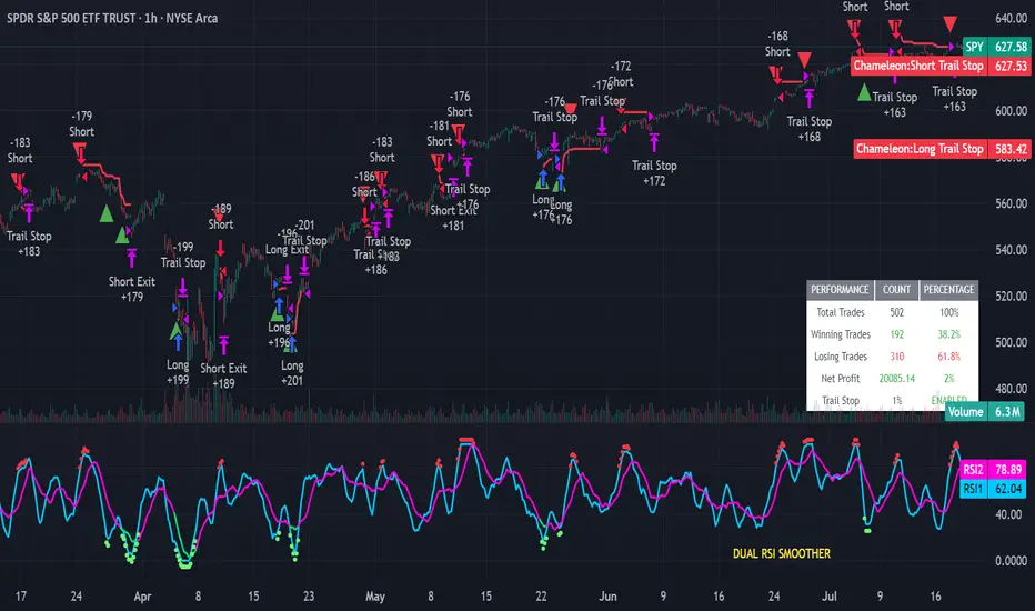
Strategy Chameleon [theUltimator5]Have you ever looked at an indicator and wondered to yourself "Is this indicator actually profitable?" Well now you can test it out for yourself with the Strategy Chameleon!
Strategy Chameleon is a versatile, signal-agnostic trading strategy designed to adapt to any external indicator or trading system. Like a chameleon changes colors to match its environment, this strategy adapts to match any buy/sell signals you provide, making it the ultimate backtesting and automation tool for traders who want to test multiple strategies without rewriting code.
🎯 Key Features
1) Connects ANY external indicator's buy/sell signals
Works with RSI, MACD, moving averages, custom indicators, or any Pine Script output
Simply connect your indicator's signal output to the strategy inputs
2) Multiple Stop Loss Types:
Percentage-based stops
ATR (Average True Range) dynamic stops
Fixed point stops
3) Advanced Trailing Stop System:
Percentage trailing
ATR-based trailing
Fixed point trailing
4) Flexible Take Profit Options:
Risk:Reward ratio targeting
Percentage-based profits
ATR-based profits
Fixed point profits
5) Trading Direction Control
Long Only - Bull market strategies
Short Only - Bear market strategies
Both - Full market strategies
6) Time-Based Filtering
Optional trading session restrictions
Customize active trading hours
Perfect for day trading strategies
📈 How It Works
Signal Detection: The strategy monitors your connected buy/sell signals
Entry Logic: Executes trades when signals trigger during valid time periods
Risk Management: Automatically applies your chosen stop loss and take profit levels
Trailing System: Dynamically adjusts stops to lock in profits
Performance Tracking: Real-time statistics table showing win rate and performance
⚙️ Setup Instructions
0) Add indicator you want to test, then add the Strategy to your chart
Connect Your Signals:
imgur.com
Go to strategy settings → Signal Sources
1) Set "Buy Signal Source" to your indicator's buy output
2) Set "Sell Signal Source" to your indicator's sell output
3) Choose table position - This simply changes the table location on the screen
4) Set trading direction preference - Buy only? Sell only? Both directions?
imgur.com
5) Set your preferred stop loss type and level
You can set the stop loss to be either percentage based or ATR and fully configurable.
6) Enable trailing stops if desired
imgur.com
7) Configure take profit settings
8) Toggle time filter to only consider specific time windows or trading sessions.
🚀 Use Cases
Test various indicators to determine feasibility and/or profitability.
Compare different signal sources quickly
Validate trading ideas with consistent risk management
Portfolio Management
Apply uniform risk management across different strategies
Standardize stop loss and take profit rules
Monitor performance consistently
Automation Ready
Built-in alert conditions for automated trading
Compatible with trading bots and webhooks
Easy integration with external systems
⚠️ Important Notes
This strategy requires external signals to function
Default settings use 10% of equity per trade
Pyramiding is disabled (one position at a time)
Strategy calculates on bar close, not every tick
🔗 Integration Examples
Works perfectly with:
RSI strategies (connect RSI > 70 for sells, RSI < 30 for buys)
Moving average crossovers
MACD signal line crosses
Bollinger Band strategies
Custom oscillators and indicators
Multi-timeframe strategies
📋 Default Settings
Position Size: 10% of equity
Stop Loss: 2% percentage-based
Trailing Stop: 1.5% percentage-based (enabled)
Take Profit: Disabled (optional)
Trade Direction: Both long and short
Time Filter: Disabled
Buy Dip Multiple Positions🎯 Objective
This strategy aims to capture aggressive dip-buying opportunities during volume-confirmed price reversals in short term downtrending markets. It is optimized for multi-entry precision, adaptive stop management, and real-time trade monitoring.
It allows traders to execute multiple long entries and dynamically trail stops to maximize gains while capping risk. Designed with modular inputs, this strategy is ideal for intraday momentum scalping and swing trading alike.
🔧 How It Operates
The strategy triggers buy entries when three conditions align:
Reversal Candle: Current close < prior low × 0.998
Volume Confirmation: Current volume exceeds average of prior 2 bars × 1.2
Price Surge Threshold: Current close below user-defined % of close from N bars ago
Once a reversal candle is confirmed, the strategy:
Calculates position size based on user-defined risk parameters
Allows up to a max number of simultaneous trades
Trailing Stop kicks in 2 bars after entry, climbing by a user-defined % each bar
Exit occurs when price hits either the trailing stop or target price
🛠️ Inputs
Users can customize all major aspects of the strategy:
Max Simultaneous Trades: Default 20
Trailing Stop Increase per Bar (%): Default 1%
Initial Stop (% of Reversal Low): Default 85%
Target Price (% Above Reversal Low): Default 60%
Price Surge Threshold (% of Past Close): Default 89%
Surge Lookback Bars: Default 14
Show Active Trade Dot: Toggle to display green trade status dot
📊 Visual Overlays
The chart displays the following:
Marker Description
🟢 Green Dot Active trade (toggleable)
🔴 Red Dot Max trades reached
📈 Trailing Stop Applied internally but not plotted (can be added)
📊 Metrics Plots of win rate, winning/losing trade counts
📎 Notes
Strategy uses strategy.cash allocation logic
Entry size adapts to account equity and risk per trade
All parameters are accessible via the settings panel
Built entirely in Pine Script v5
This strategy balances flexibility and precision, giving traders control over entry timing, capital allocation, and stop behavior. Ideal for those looking to automate dip-buy setups with tactical overlays and visual alerts.

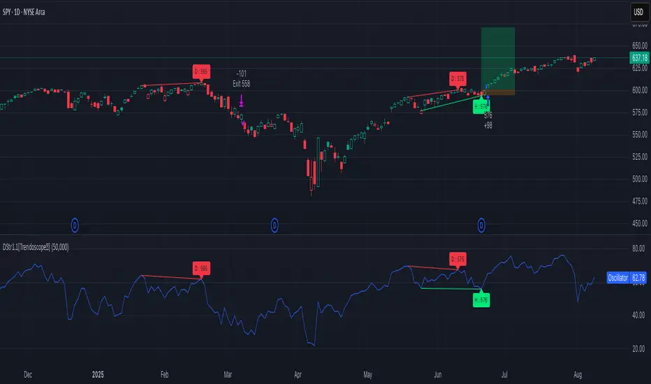
Divergence Strategy [Trendoscope®]🎲 Overview
The Divergence Strategy is a sophisticated TradingView strategy that enhances the Divergence Screener by adding automated trade signal generation, risk management, and trade visualization. It leverages the screener’s robust divergence detection to identify bullish, bearish, regular, and hidden divergences, then executes trades with precise entry, stop-loss, and take-profit levels. Designed for traders seeking automated trading solutions, this strategy offers customizable trade parameters and visual feedback to optimize performance across various markets and timeframes.
For core divergence detection features, including oscillator options, trend detection methods, zigzag pivot analysis, and visualization, refer to the Divergence Screener documentation. This description focuses on the strategy-specific enhancements for automated trading and risk management.
🎲 Strategy Features
🎯Automated Trade Signal Generation
Trade Direction Control : Restrict trades to long-only or short-only to align with market bias or strategy goals, preventing conflicting orders.
Divergence Type Selection : Choose to trade regular divergences (bullish/bearish), hidden divergences, or both, targeting reversals or trend continuations.
Entry Type Options :
Cautious : Enters conservatively at pivot points and exits quickly to minimize risk exposure.
Confident : Enters aggressively at the latest price and holds longer to capture larger moves.
Mixed : Combines conservative entries with delayed exits for a balanced approach.
Market vs. Stop Orders: Opt for market orders for instant execution or stop orders for precise price entry.
🎯 Enhanced Risk Management
Risk/Reward Ratio : Define a risk-reward ratio (default: 2.0) to set profit targets relative to stop-loss levels, ensuring consistent trade sizing.
Bracket Orders : Trades include entry, stop-loss, and take-profit levels calculated from divergence pivot points, tailored to the entry type and risk-reward settings.
Stop-Loss Placement : Stops are strategically set (e.g., at recent pivot or last price point) based on entry type, balancing risk and trade validity.
Order Cancellation : Optionally cancel pending orders when a divergence is broken (e.g., price moves past the pivot in the wrong direction), reducing invalid trades. This feature is toggleable for flexibility.
🎯 Trade Visualization
Target and Stop Boxes : Displays take-profit (lime) and stop-loss (orange) levels as boxes on the price chart, extending 10 bars forward for clear visibility.
Dynamic Trade Updates : Trade visualizations are added, updated, or removed as trades are executed, canceled, or invalidated, ensuring accurate feedback.
Overlay Integration : Trade levels overlay the price chart, complementing the screener’s oscillator-based divergence lines and labels.
🎯 Strategy Default Configuration
Capital and Sizing : Set initial capital (default: $1,000,000) and position size (default: 20% of equity) for realistic backtesting.
Pyramiding : Allows up to 4 concurrent trades, enabling multiple divergence-based entries in trending markets.
Commission and Margin : Accounts for commission (default: 0.01%) and margin (100% for long/short) to reflect trading costs.
Performance Optimization : Processes up to 5,000 bars dynamically, balancing historical analysis and real-time execution.
🎲 Inputs and Configuration
🎯Trade Settings
Direction : Select Long or Short (default: Long).
Divergence : Trade Regular, Hidden, or Both divergence types (default: Both).
Entry/Exit Type : Choose Cautious, Confident, or Mixed (default: Cautious).
Risk/Reward : Set the risk-reward ratio for profit targets (default: 2.0).
Use Market Order : Enable market orders for immediate entry (default: false, uses limit orders).
Cancel On Break : Cancel pending orders when divergence is broken (default: true).
🎯Inherited Settings
The strategy inherits all inputs from the Divergence Screener, including:
Oscillator Settings : Oscillator type (e.g., RSI, CCI), length, and external oscillator option.
Trend Settings : Trend detection method (Zigzag, MA Difference, External), MA type, and length.
Zigzag Settings : Zigzag length (fixed repaint = true).
🎲 Entry/Exit Types for Divergence Scenarios
The Divergence Strategy offers three Entry/Exit Type options—Cautious, Confident, and Mixed—which determine how trades are entered and exited based on divergence pivot points. This section explains how these settings apply to different divergence scenarios, with placeholders for screenshots to illustrate each case.
The divergence pattern forms after 3 pivots. The stop and entry levels are formed on one of these levels based on Entry/Exit types.
🎯Bullish Divergence (Reversal)
A bullish divergence occurs when price forms a lower low, but the oscillator forms a higher low, signaling a potential upward reversal.
💎 Cautious:
Entry : At the pivot high point for a conservative entry.
Exit : Stop-loss at the last pivot point (previous low that is higher than the current pivot low); take-profit at risk-reward ratio. Canceled if price breaks below the pivot (if Cancel On Break is enabled).
Behavior : Enters after confirmation and exits quickly to limit downside risk.
💎Confident:
Entry : At the last pivot low, (previous low which is higher than the current pivot low) for an aggressive entry.
Exit : Stop-loss at recent pivot low, which is the lowest point; take-profit at risk-reward ratio. Canceled if price breaks below the pivot. (lazy exit)
Behavior : Enters early to capture trend continuation, holding longer for gains.
💎Mixed:
Entry : At the pivot high point (conservative).
Exit : Stop-loss at the recent pivot point that has resulted in lower low (lazy exit). Canceled if price breaks below the pivot.
Behavior : Balances entry caution with extended holding for trend continuation.
🎯Bearish Divergence (Reversal)
A bearish divergence occurs when price forms a higher high, but the oscillator forms a lower high, indicating a potential downward reversal.
💎Cautious:
Entry : At the pivot low point (lower high) for a conservative short entry.
Exit : Stop-loss at the previous pivot high point (previous high); take-profit at risk-reward ratio. Canceled if price breaks above the pivot (if Cancel On Break is enabled).
Behavior : Enters conservatively and exits quickly to minimize risk.
💎Confident:
Entry : At the last price point (previous high) for an aggressive short entry.
Exit : Stop-loss at the pivot point; take-profit at risk-reward ratio. Canceled if price breaks above the pivot.
Behavior : Enters early to maximize trend continuation, holding longer.
💎Mixed:
Entry : At the previous piot high point (conservative).
Exit : Stop-loss at the last price point (delayed exit). Canceled if price breaks above the pivot.
Behavior : Combines conservative entry with extended holding for downtrend gains.
🎯Bullish Hidden Divergence (Continuation)
A bullish hidden divergence occurs when price forms a higher low, but the oscillator forms a lower low, suggesting uptrend continuation. In case of Hidden bullish divergence, b]Entry is always on the previous pivot high (unless it is a market order)
💎Cautious:
Exit : Stop-loss at the recent pivot low point (higher than previous pivot low); take-profit at risk-reward ratio. Canceled if price breaks below the pivot (if Cancel On Break is enabled).
Behavior : Enters after confirmation and exits quickly to limit downside risk.
💎Confident:
Exit : Stop-loss at previous pivot low, which is the lowest point; take-profit at risk-reward ratio. Canceled if price breaks below the pivot. (lazy exit)
Behavior : Enters early to capture trend continuation, holding longer for gains.
🎯Bearish Hidden Divergence (Continuation)
A bearish hidden divergence occurs when price forms a lower high, but the oscillator forms a higher high, suggesting downtrend continuation. In case of Hidden Bearish divergence, b]Entry is always on the previous pivot low (unless it is a market order)
💎Cautious:
Exit : Stop-loss at the latest pivot high point (which is a lower high); take-profit at risk-reward ratio. Canceled if price breaks above the pivot (if Cancel On Break is enabled).
Behavior : Enters conservatively and exits quickly to minimize risk.
💎Confident/Mixed:
Exit : Stop-loss at the previous pivot high point; take-profit at risk-reward ratio. Canceled if price breaks above the pivot.
Behavior : Uses the late exit point to hold longer.
🎲 Usage Instructions
🎯Add to Chart:
Add the Divergence Strategy to your TradingView chart.
The oscillator and divergence signals appear in a separate pane, with trade levels (target/stop boxes) overlaid on the price chart.
🎯Configure Settings:
Adjust trade settings (direction, divergence type, entry type, risk-reward, market orders, cancel on break).
Modify inherited Divergence Screener settings (oscillator, trend method, zigzag length) as needed.
Enable/disable alerts for divergence notifications.
🎯Interpret Signals:
Long Trades: Triggered on bullish or bullish hidden divergences (if allowed), shown with green/lime lines and labels.
Short Trades: Triggered on bearish or bearish hidden divergences (if allowed), shown with red/orange lines and labels.
Monitor lime (target) and orange (stop) boxes for trade levels.
Review strategy performance metrics (e.g., profit/loss, win rate) in the strategy tester.
🎯Backtest and Optimize:
Use TradingView’s strategy tester to evaluate performance on historical data.
Fine-tune risk-reward, entry type, position sizing, and cancellation settings to suit your market and timeframe.
For questions, suggestions, or support, contact Trendoscope via TradingView or official support channels. Stay tuned for updates and enhancements to the Divergence Strategy!
Holy GrailThis is a long-only educational strategy that simulates what happens if you keep adding to a position during pullbacks and only exit when the asset hits a new All-Time High (ATH). It is intended for learning purposes only — not for live trading.
🧠 How it works:
The strategy identifies pullbacks using a simple moving average (MA).
When price dips below the MA, it begins monitoring for the first green candle (close > open).
That green candle signals a potential bottom, so it adds to the position.
If price goes lower, it waits for the next green candle and adds again.
The exit happens after ATH — it sells on each red candle (close < open) once a new ATH is reached.
You can adjust:
MA length (defines what’s considered a pullback)
Initial buy % (how much to pre-fill before signals start)
Buy % per signal (after pullback green candle)
Exit % per red candle after ATH
📊 Intended assets & timeframes:
This strategy is designed for broad market indices and long-term appreciating assets, such as:
SPY, NASDAQ, DAX, FTSE
Use it only on 1D or higher timeframes — it’s not meant for scalping or short-term trading.
⚠️ Important Limitations:
Long-only: The script does not short. It assumes the asset will eventually recover to a new ATH.
Not for all assets: It won't work on assets that may never recover (e.g., single stocks or speculative tokens).
Slow capital deployment: Entries happen gradually and may take a long time to close.
Not optimized for returns: Buy & hold can outperform this strategy.
No slippage, fees, or funding costs included.
This is not a performance strategy. It’s a teaching tool to show that:
High win rate ≠ high profitability
Patience can be deceiving
Many signals = long capital lock-in
🎓 Why it exists:
The purpose of this strategy is to demonstrate market psychology and risk overconfidence. Traders often chase strategies with high win rates without considering holding time, drawdowns, or opportunity cost.
This script helps visualize that phenomenon.

Anomalous Holonomy Field Theory🌌 Anomalous Holonomy Field Theory (AHFT) - Revolutionary Quantum Market Analysis
Where Theoretical Physics Meets Trading Reality
A Groundbreaking Synthesis of Differential Geometry, Quantum Field Theory, and Market Dynamics
🔬 THEORETICAL FOUNDATION - THE MATHEMATICS OF MARKET REALITY
The Anomalous Holonomy Field Theory represents an unprecedented fusion of advanced mathematical physics with practical market analysis. This isn't merely another indicator repackaging old concepts - it's a fundamentally new lens through which to view and understand market structure .
1. HOLONOMY GROUPS (Differential Geometry)
In differential geometry, holonomy measures how vectors change when parallel transported around closed loops in curved space. Applied to markets:
Mathematical Formula:
H = P exp(∮_C A_μ dx^μ)
Where:
P = Path ordering operator
A_μ = Market connection (price-volume gauge field)
C = Closed price path
Market Implementation:
The holonomy calculation measures how price "remembers" its journey through market space. When price returns to a previous level, the holonomy captures what has changed in the market's internal geometry. This reveals:
Hidden curvature in the market manifold
Topological obstructions to arbitrage
Geometric phase accumulated during price cycles
2. ANOMALY DETECTION (Quantum Field Theory)
Drawing from the Adler-Bell-Jackiw anomaly in quantum field theory:
Mathematical Formula:
∂_μ j^μ = (e²/16π²)F_μν F̃^μν
Where:
j^μ = Market current (order flow)
F_μν = Field strength tensor (volatility structure)
F̃^μν = Dual field strength
Market Application:
Anomalies represent symmetry breaking in market structure - moments when normal patterns fail and extraordinary opportunities arise. The system detects:
Spontaneous symmetry breaking (trend reversals)
Vacuum fluctuations (volatility clusters)
Non-perturbative effects (market crashes/melt-ups)
3. GAUGE THEORY (Theoretical Physics)
Markets exhibit gauge invariance - the fundamental physics remains unchanged under certain transformations:
Mathematical Formula:
A'_μ = A_μ + ∂_μΛ
This ensures our signals are gauge-invariant observables , immune to arbitrary market "coordinate changes" like gaps or reference point shifts.
4. TOPOLOGICAL DATA ANALYSIS
Using persistent homology and Morse theory:
Mathematical Formula:
β_k = dim(H_k(X))
Where β_k are the Betti numbers describing topological features that persist across scales.
🎯 REVOLUTIONARY SIGNAL CONFIGURATION
Signal Sensitivity (0.5-12.0, default 2.5)
Controls the responsiveness of holonomy field calculations to market conditions. This parameter directly affects the threshold for detecting quantum phase transitions in price action.
Optimization by Timeframe:
Scalping (1-5min): 1.5-3.0 for rapid signal generation
Day Trading (15min-1H): 2.5-5.0 for balanced sensitivity
Swing Trading (4H-1D): 5.0-8.0 for high-quality signals only
Score Amplifier (10-200, default 50)
Scales the raw holonomy field strength to produce meaningful signal values. Higher values amplify weak signals in low-volatility environments.
Signal Confirmation Toggle
When enabled, enforces additional technical filters (EMA and RSI alignment) to reduce false positives. Essential for conservative strategies.
Minimum Bars Between Signals (1-20, default 5)
Prevents overtrading by enforcing quantum decoherence time between signals. Higher values reduce whipsaws in choppy markets.
👑 ELITE EXECUTION SYSTEM
Execution Modes:
Conservative Mode:
Stricter signal criteria
Higher quality thresholds
Ideal for stable market conditions
Adaptive Mode:
Self-adjusting parameters
Balances signal frequency with quality
Recommended for most traders
Aggressive Mode:
Maximum signal sensitivity
Captures rapid market moves
Best for experienced traders in volatile conditions
Dynamic Position Sizing:
When enabled, the system scales position size based on:
Holonomy field strength
Current volatility regime
Recent performance metrics
Advanced Exit Management:
Implements trailing stops based on ATR and signal strength, with mode-specific multipliers for optimal profit capture.
🧠 ADAPTIVE INTELLIGENCE ENGINE
Self-Learning System:
The strategy analyzes recent trade outcomes and adjusts:
Risk multipliers based on win/loss ratios
Signal weights according to performance
Market regime detection for environmental adaptation
Learning Speed (0.05-0.3):
Controls adaptation rate. Higher values = faster learning but potentially unstable. Lower values = stable but slower adaptation.
Performance Window (20-100 trades):
Number of recent trades analyzed for adaptation. Longer windows provide stability, shorter windows increase responsiveness.
🎨 REVOLUTIONARY VISUAL SYSTEM
1. Holonomy Field Visualization
What it shows: Multi-layer quantum field bands representing market resonance zones
How to interpret:
Blue/Purple bands = Primary holonomy field (strongest resonance)
Band width = Field strength and volatility
Price within bands = Normal quantum state
Price breaking bands = Quantum phase transition
Trading application: Trade reversals at band extremes, breakouts on band violations with strong signals.
2. Quantum Portals
What they show: Entry signals with recursive depth patterns indicating momentum strength
How to interpret:
Upward triangles with portals = Long entry signals
Downward triangles with portals = Short entry signals
Portal depth = Signal strength and expected momentum
Color intensity = Probability of success
Trading application: Enter on portal appearance, with size proportional to portal depth.
3. Field Resonance Bands
What they show: Fibonacci-based harmonic price zones where quantum resonance occurs
How to interpret:
Dotted circles = Minor resonance levels
Solid circles = Major resonance levels
Color coding = Resonance strength
Trading application: Use as dynamic support/resistance, expect reactions at resonance zones.
4. Anomaly Detection Grid
What it shows: Fractal-based support/resistance with anomaly strength calculations
How to interpret:
Triple-layer lines = Major fractal levels with high anomaly probability
Labels show: Period (H8-H55), Price, and Anomaly strength (φ)
⚡ symbol = Extreme anomaly detected
● symbol = Strong anomaly
○ symbol = Normal conditions
Trading application: Expect major moves when price approaches high anomaly levels. Use for precise entry/exit timing.
5. Phase Space Flow
What it shows: Background heatmap revealing market topology and energy
How to interpret:
Dark background = Low market energy, range-bound
Purple glow = Building energy, trend developing
Bright intensity = High energy, strong directional move
Trading application: Trade aggressively in bright phases, reduce activity in dark phases.
📊 PROFESSIONAL DASHBOARD METRICS
Holonomy Field Strength (-100 to +100)
What it measures: The Wilson loop integral around price paths
>70: Strong positive curvature (bullish vortex)
<-70: Strong negative curvature (bearish collapse)
Near 0: Flat connection (range-bound)
Anomaly Level (0-100%)
What it measures: Quantum vacuum expectation deviation
>70%: Major anomaly (phase transition imminent)
30-70%: Moderate anomaly (elevated volatility)
<30%: Normal quantum fluctuations
Quantum State (-1, 0, +1)
What it measures: Market wave function collapse
+1: Bullish eigenstate |↑⟩
0: Superposition (uncertain)
-1: Bearish eigenstate |↓⟩
Signal Quality Ratings
LEGENDARY: All quantum fields aligned, maximum probability
EXCEPTIONAL: Strong holonomy with anomaly confirmation
STRONG: Good field strength, moderate anomaly
MODERATE: Decent signals, some uncertainty
WEAK: Minimal edge, high quantum noise
Performance Metrics
Win Rate: Rolling performance with emoji indicators
Daily P&L: Real-time profit tracking
Adaptive Risk: Current risk multiplier status
Market Regime: Bull/Bear classification
🏆 WHY THIS CHANGES EVERYTHING
Traditional technical analysis operates on 100-year-old principles - moving averages, support/resistance, and pattern recognition. These work because many traders use them, creating self-fulfilling prophecies.
AHFT transcends this limitation by analyzing markets through the lens of fundamental physics:
Markets have geometry - The holonomy calculations reveal this hidden structure
Price has memory - The geometric phase captures path-dependent effects
Anomalies are predictable - Quantum field theory identifies symmetry breaking
Everything is connected - Gauge theory unifies disparate market phenomena
This isn't just a new indicator - it's a new way of thinking about markets . Just as Einstein's relativity revolutionized physics beyond Newton's mechanics, AHFT revolutionizes technical analysis beyond traditional methods.
🔧 OPTIMAL SETTINGS FOR MNQ 10-MINUTE
For the Micro E-mini Nasdaq-100 on 10-minute timeframe:
Signal Sensitivity: 2.5-3.5
Score Amplifier: 50-70
Execution Mode: Adaptive
Min Bars Between: 3-5
Theme: Quantum Nebula or Dark Matter
💭 THE JOURNEY - FROM IMPOSSIBLE THEORY TO TRADING REALITY
Creating AHFT was a mathematical odyssey that pushed the boundaries of what's possible in Pine Script. The journey began with a seemingly impossible question: Could the profound mathematical structures of theoretical physics be translated into practical trading tools?
The Theoretical Challenge:
Months were spent diving deep into differential geometry textbooks, studying the works of Chern, Simons, and Witten. The mathematics of holonomy groups and gauge theory had never been applied to financial markets. Translating abstract mathematical concepts like parallel transport and fiber bundles into discrete price calculations required novel approaches and countless failed attempts.
The Computational Nightmare:
Pine Script wasn't designed for quantum field theory calculations. Implementing the Wilson loop integral, managing complex array structures for anomaly detection, and maintaining computational efficiency while calculating geometric phases pushed the language to its limits. There were moments when the entire project seemed impossible - the script would timeout, produce nonsensical results, or simply refuse to compile.
The Breakthrough Moments:
After countless sleepless nights and thousands of lines of code, breakthrough came through elegant simplifications. The realization that market anomalies follow patterns similar to quantum vacuum fluctuations led to the revolutionary anomaly detection system. The discovery that price paths exhibit holonomic memory unlocked the geometric phase calculations.
The Visual Revolution:
Creating visualizations that could represent 4-dimensional quantum fields on a 2D chart required innovative approaches. The multi-layer holonomy field, recursive quantum portals, and phase space flow representations went through dozens of iterations before achieving the perfect balance of beauty and functionality.
The Balancing Act:
Perhaps the greatest challenge was maintaining mathematical rigor while ensuring practical trading utility. Every formula had to be both theoretically sound and computationally efficient. Every visual had to be both aesthetically pleasing and information-rich.
The result is more than a strategy - it's a synthesis of pure mathematics and market reality that reveals the hidden order within apparent chaos.
📚 INTEGRATED DOCUMENTATION
Once applied to your chart, AHFT includes comprehensive tooltips on every input parameter. The source code contains detailed explanations of the mathematical theory, practical applications, and optimization guidelines. This published description provides the overview - the indicator itself is a complete educational resource.
⚠️ RISK DISCLAIMER
While AHFT employs advanced mathematical models derived from theoretical physics, markets remain inherently unpredictable. No mathematical model, regardless of sophistication, can guarantee future results. This strategy uses realistic commission ($0.62 per contract) and slippage (1 tick) in all calculations. Past performance does not guarantee future results. Always use appropriate risk management and never risk more than you can afford to lose.
🌟 CONCLUSION
The Anomalous Holonomy Field Theory represents a quantum leap in technical analysis - literally. By applying the profound insights of differential geometry, quantum field theory, and gauge theory to market analysis, AHFT reveals structure and opportunities invisible to traditional methods.
From the holonomy calculations that capture market memory to the anomaly detection that identifies phase transitions, from the adaptive intelligence that learns and evolves to the stunning visualizations that make the invisible visible, every component works in mathematical harmony.
This is more than a trading strategy. It's a new lens through which to view market reality.
Trade with the precision of physics. Trade with the power of mathematics. Trade with AHFT.
I hope this serves as a good replacement for Quantum Edge Pro - Adaptive AI until I'm able to fix it.
— Dskyz, Trade with insight. Trade with anticipation.

Volume Momentum [BackQuant]Volume Momentum
The Volume Momentum indicator is designed to help traders identify shifts in market momentum based on volume data. By analyzing the relative volume momentum, this indicator provides insights into whether the market is gaining strength (uptrend) or losing momentum (downtrend). The strategy uses a combination of percentile-based volume normalization, weighted moving averages (WMA), and exponential moving averages (EMA) to assess volume trends.
The system focuses on the relationship between price and volume, utilizing normalized volume data to highlight key market changes. This approach allows traders to focus on volume-driven price movements, helping them to capture momentum shifts early.
Key Features
1. Volume Normalization and Percentile Calculation:
The signed volume (positive when the close is higher than the open, negative when the close is lower) is normalized against the rolling average volume. This normalized volume is then subjected to a percentile interpolation, allowing for a robust statistical measure of how the current volume compares to historical data. The percentile level is customizable, with 50 representing the median.
2. Weighted and Smoothed Moving Averages for Trend Detection:
The normalized volume is smoothed using weighted moving averages (WMA) and exponential moving averages (EMA). These smoothing techniques help eliminate noise, providing a clearer view of the underlying momentum. The WMA filters out short-term fluctuations, while the EMA ensures that the most recent data points have a higher weight, making the system more responsive to current market conditions.
3. Trend Reversal Detection:
The indicator detects momentum shifts by evaluating whether the volume momentum crosses above or below zero. A positive volume momentum indicates a potential uptrend, while a negative momentum suggests a possible downtrend. These trend reversals are identified through crossover and crossunder conditions, triggering alerts when significant changes occur.
4. Dynamic Trend Background and Bar Coloring:
The script offers customizable background coloring based on the trend direction. When volume momentum is positive, the background is colored green, indicating a bullish trend. When volume momentum is negative, the background is colored red, signaling a bearish trend. Additionally, the bars themselves can be colored based on the trend, further helping traders quickly visualize market momentum.
5. Alerts for Momentum Shifts:
The system provides real-time alerts for traders to monitor when volume momentum crosses a critical threshold (zero), signaling a trend reversal. The alerts notify traders when the market momentum turns bullish or bearish, assisting them in making timely decisions.
6. Customizable Parameters for Flexible Usage:
Users can fine-tune the behavior of the indicator by adjusting various parameters:
Volume Rolling Mean: The period used to calculate the average volume for normalization.
Percentile Interpolation Length: Defines the range over which the percentile is calculated.
Percentile Level: Determines the percentile threshold (e.g., 50 for the median).
WMA and Smoothing Periods: Control the smoothing and response time of the indicator.
7. Trend Background Visualization and Trend-Based Bar Coloring:
The background fill is shaded according to whether the volume momentum is positive or negative, providing a visual cue to indicate market strength. Additionally, bars can be color-coded to highlight the trend, making it easier to see the trend’s direction without needing to analyze numerical data manually.
8. Note on Mean-Reversion Strategy:
If you take the inverse of the signals, this indicator can be adapted for a mean-reversion strategy. Instead of following the trend, the strategy would involve buying assets that are underperforming and selling assets that are overperforming, based on volume momentum. However, it’s important to note that this approach may not work effectively on highly correlated assets, as their price movements may be too similar, reducing the effectiveness of the mean-reversion strategy.
Final Thoughts
The Volume Momentum indicator offers a comprehensive approach to analyzing volume-based momentum shifts in the market. By using volume normalization, percentile interpolation, and smoothed moving averages, this system helps identify the strength and direction of market trends. Whether used for trend-following or adapted for mean-reversion, this tool provides traders with actionable insights into the market’s volume-driven movements, improving decision-making and portfolio management.

Performance Metrics With Bracketed Rebalacing [BackQuant]Performance Metrics With Bracketed Rebalancing
The Performance Metrics With Bracketed Rebalancing script offers a robust method for assessing portfolio performance, integrating advanced portfolio metrics with different rebalancing strategies. With a focus on adaptability, the script allows traders to monitor and adjust portfolio weights, equity, and other key financial metrics dynamically. This script provides a versatile approach for evaluating different trading strategies, considering factors like risk-adjusted returns, volatility, and the impact of portfolio rebalancing.
Please take the time to read the following:
Key Features and Benefits of Portfolio Methods
Bracketed Rebalancing:
Bracketed Rebalancing is an advanced strategy designed to trigger portfolio adjustments when an asset's weight surpasses a predefined threshold. This approach minimizes overexposure to any single asset while maintaining flexibility in response to market changes. The strategy is particularly beneficial for mitigating risks that arise from significant asset weight fluctuations. The following image illustrates how this method reacts when asset weights cross the threshold:
Daily Rebalancing:
Unlike the bracketed method, Daily Rebalancing adjusts portfolio weights every trading day, ensuring consistent asset allocation. This method aims for a more even distribution of portfolio weights, making it a suitable option for traders who prefer less sensitivity to individual asset volatility. Here's an example of Daily Rebalancing in action:
No Rebalancing:
For traders who prefer a passive approach, the "No Rebalancing" option allows the portfolio to remain static, without any adjustments to asset weights. This method may appeal to long-term investors or those who believe in the inherent stability of their selected assets. Here’s how the portfolio looks when no rebalancing is applied:
Portfolio Weights Visualization:
One of the standout features of this script is the visual representation of portfolio weights. With adjustable settings, users can track the current allocation of assets in real-time, making it easier to analyze shifts and trends. The following image shows the real-time weight distribution across three assets:
Rolling Drawdown Plot:
Managing drawdown risk is a critical aspect of portfolio management. The Rolling Drawdown Plot visually tracks the drawdown over time, helping traders monitor the risk exposure and performance relative to the peak equity levels. This feature is essential for assessing the portfolio's resilience during market downturns:
Daily Portfolio Returns:
Tracking daily returns is crucial for evaluating the short-term performance of the portfolio. The script allows users to plot daily portfolio returns to gain insights into daily profit or loss, helping traders stay updated on their portfolio’s progress:
Performance Metrics
Net Profit (%):
This metric represents the total return on investment as a percentage of the initial capital. A positive net profit indicates that the portfolio has gained value over the evaluation period, while a negative value suggests a loss. It's a fundamental indicator of overall portfolio performance.
Maximum Drawdown (Max DD):
Maximum Drawdown measures the largest peak-to-trough decline in portfolio value during a specified period. It quantifies the most significant loss an investor would have experienced if they had invested at the highest point and sold at the lowest point within the timeframe. A smaller Max DD indicates better risk management and less exposure to significant losses.
Annual Mean Returns (% p/y):
This metric calculates the average annual return of the portfolio over the evaluation period. It provides insight into the portfolio's ability to generate returns on an annual basis, aiding in performance comparison with other investment opportunities.
Annual Standard Deviation of Returns (% p/y):
This measure indicates the volatility of the portfolio's returns on an annual basis. A higher standard deviation signifies greater variability in returns, implying higher risk, while a lower value suggests more stable returns.
Variance:
Variance is the square of the standard deviation and provides a measure of the dispersion of returns. It helps in understanding the degree of risk associated with the portfolio's returns.
Sortino Ratio:
The Sortino Ratio is a variation of the Sharpe Ratio that only considers downside risk, focusing on negative volatility. It is calculated as the difference between the portfolio's return and the minimum acceptable return (MAR), divided by the downside deviation. A higher Sortino Ratio indicates better risk-adjusted performance, emphasizing the importance of avoiding negative returns.
Sharpe Ratio:
The Sharpe Ratio measures the portfolio's excess return per unit of total risk, as represented by standard deviation. It is calculated by subtracting the risk-free rate from the portfolio's return and dividing by the standard deviation of the portfolio's excess return. A higher Sharpe Ratio indicates more favorable risk-adjusted returns.
Omega Ratio:
The Omega Ratio evaluates the probability of achieving returns above a certain threshold relative to the probability of experiencing returns below that threshold. It is calculated by dividing the cumulative probability of positive returns by the cumulative probability of negative returns. An Omega Ratio greater than 1 indicates a higher likelihood of achieving favorable returns.
Gain-to-Pain Ratio:
The Gain-to-Pain Ratio measures the return per unit of risk, focusing on the magnitude of gains relative to the severity of losses. It is calculated by dividing the total gains by the total losses experienced during the evaluation period. A higher ratio suggests a more favorable balance between reward and risk.
www.linkedin.com
Compound Annual Growth Rate (CAGR) (% p/y):
CAGR represents the mean annual growth rate of the portfolio over a specified period, assuming the investment has been compounding over that time. It provides a smoothed annual rate of growth, eliminating the effects of volatility and offering a clearer picture of long-term performance.
Portfolio Alpha (% p/y):
Portfolio Alpha measures the portfolio's performance relative to a benchmark index, adjusting for risk. It is calculated using the Capital Asset Pricing Model (CAPM) and represents the excess return of the portfolio over the expected return based on its beta and the benchmark's performance. A positive alpha indicates outperformance, while a negative alpha suggests underperformance.
Portfolio Beta:
Portfolio Beta assesses the portfolio's sensitivity to market movements, indicating its exposure to systematic risk. A beta greater than 1 suggests the portfolio is more volatile than the market, while a beta less than 1 indicates lower volatility. Beta is used to understand the portfolio's potential for gains or losses in relation to market fluctuations.
Skewness of Returns:
Skewness measures the asymmetry of the return distribution. A positive skew indicates a distribution with a long right tail, suggesting more frequent small losses and fewer large gains. A negative skew indicates a long left tail, implying more frequent small gains and fewer large losses. Understanding skewness helps in assessing the likelihood of extreme outcomes.
Value at Risk (VaR) 95th Percentile:
VaR at the 95th percentile estimates the maximum potential loss over a specified period, given a 95% confidence level. It provides a threshold value such that there is a 95% probability that the portfolio will not experience a loss greater than this amount.
Conditional Value at Risk (CVaR):
CVaR, also known as Expected Shortfall, measures the average loss exceeding the VaR threshold. It provides insight into the tail risk of the portfolio, indicating the expected loss in the worst-case scenarios beyond the VaR level.
These metrics collectively offer a comprehensive view of the portfolio's performance, risk exposure, and efficiency. By analyzing these indicators, investors can make informed decisions, balancing potential returns with acceptable levels of risk.
Conclusion
The Performance Metrics With Bracketed Rebalancing script provides a comprehensive framework for evaluating and optimizing portfolio performance. By integrating advanced metrics, adaptive rebalancing strategies, and visual analytics, it empowers traders to make informed decisions in managing their investment portfolios. However, it's crucial to consider the implications of rebalancing strategies, as academic research indicates that predictable rebalancing can lead to market impact costs. Therefore, adopting flexible and less predictable rebalancing approaches may enhance portfolio performance and reduce associated costs.
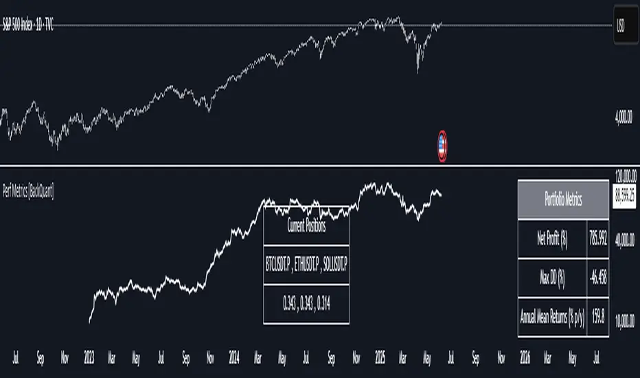
System 0530 - Stoch RSI Strategy with ATR filterStrategy Description: System 0530 - Multi-Timeframe Stochastic RSI with ATR Filter
Overview:
This strategy, "System 0530," is designed to identify trading opportunities by leveraging the Stochastic RSI indicator across two different timeframes: a shorter timeframe for initial signal triggers (assumed to be the chart's current timeframe, e.g., 5-minute) and a longer timeframe (15-minute) for signal confirmation. It incorporates an ATR (Average True Range) filter to help ensure trades are taken during periods of adequate market volatility and includes a cooldown mechanism to prevent rapid, successive signals in the same direction. Trade exits are primarily handled by reversing signals.
How It Works:
1. Signal Initiation (e.g., 5-Minute Timeframe):
Long Signal Wait: A potential long entry is considered when the 5-minute Stochastic RSI %K line crosses above its %D line, AND the %K value at the time of the cross is at or below a user-defined oversold level (default: 30).
Short Signal Wait: A potential short entry is considered when the 5-minute Stochastic RSI %K line crosses below its %D line, AND the %K value at the time of the cross is at or above a user-defined overbought level (default: 70). When these conditions are met, the strategy enters a "waiting state" for confirmation from the 15-minute timeframe.
2. Signal Confirmation (15-Minute Timeframe):
Once in a waiting state, the strategy looks for confirmation on the 15-minute Stochastic RSI within a user-defined number of 5-minute bars (wait_window_5min_bars, default: 5 bars).
Long Confirmation:
The 15-minute Stochastic RSI %K must be greater than or equal to its %D line.
The 15-minute Stochastic RSI %K value must be below a user-defined threshold (stoch_15min_long_entry_level, default: 40).
Short Confirmation:
The 15-minute Stochastic RSI %K must be less than or equal to its %D line.
The 15-minute Stochastic RSI %K value must be above a user-defined threshold (stoch_15min_short_entry_level, default: 60).
3. Filters:
ATR Volatility Filter: If enabled, trades are only confirmed if the current ATR value (converted to ticks) is above a user-defined minimum threshold (min_atr_value_ticks). This helps to avoid taking signals during periods of very low market volatility. If the ATR condition is not met, the strategy continues to wait for the condition to be met within the confirmation window, provided other conditions still hold.
Signal Cooldown Filter: If enabled, after a signal is generated, the strategy will wait for a minimum number of bars (min_bars_between_signals) before allowing another signal in the same direction. This aims to reduce overtrading.
4. Entry and Exit Logic:
Entry: A strategy.entry() order is placed when all trigger, confirmation, and filter conditions are met.
Exit: This strategy primarily uses reversing signals for exits. For example, if a long position is open, a confirmed short signal will close the long position and open a new short position. There are no explicit take profit or stop loss orders programmed into this version of the script.
Key User-Adjustable Parameters:
Stochastic RSI Parameters: RSI Length, Stochastic RSI Length, %K Smoothing, %D Smoothing.
Signal Trigger & Confirmation:
5-minute %K trigger levels for long and short.
15-minute %K confirmation thresholds for long and short.
Wait window (in 5-minute bars) for 15-minute confirmation.
Filters:
Enable/disable and configure the Signal Cooldown filter (minimum bars between signals).
Enable/disable and configure the ATR Volatility filter (ATR period, minimum ATR value in ticks).
Strategy Parameters:
Leverage Multiplier (Note: This primarily affects theoretical position sizing for backtesting calculations in TradingView and does not simulate actual leveraged trading risks).
Recommendations for Users:
Thorough Backtesting: Test this strategy extensively on historical data for the instruments and timeframes you intend to trade.
Parameter Optimization: Experiment with different parameter settings to find what works best for your trading style and chosen markets. The default values are starting points and may not be optimal for all conditions.
Understand the Logic: Ensure you understand how each component (Stochastic RSI on different timeframes, ATR filter, cooldown) interacts to generate signals.
Risk Management: Since this version does not include explicit stop-loss orders, ensure you have a clear risk management plan in place if trading this strategy live. You might consider manually adding stop-loss orders through your broker or using TradingView's separate strategy order settings for stop-loss if applicable.
Disclaimer:
This strategy description is for informational purposes only and does not constitute financial advice. Past performance is not indicative of future results. Trading involves significant risk of loss. Always do your own research and understand the risks before trading.

Grid TLong V1The “Grid TLong V1” strategy is based on the classic Grid strategy, but in the mode of buying and selling in favor of the trend and only on Long. This allows to take advantage of large uptrend movements to maximize profits in bull markets. For this reason, excessively sideways or bearish markets may not be very conducive to this strategy.
Like our Grid strategies in favor of the trend, you can enter and exit with the balance with controlled risk, as the distance between each grid functions as a natural and adaptable stop loss and take profit. What differentiates it from bidirectional strategies is that Short uses a minimum amount of follow-through, so that the percentage distance between the grids is maintained.
In this version of the script the entries and exits can be chosen at market or limit , and are based on the profit or loss of the current position, not on the percentage change in price.
The user may also notice that the strategy setup is risk-controlled, because it risks 5% on each trade, has a fairly standard commission and modest initial capital, all in order to protect the strategy user from unrealistic results.
As with all strategies, it is strongly recommended to optimize the parameters for the strategy to be effective for each asset and for each time frame.

Dskyz (DAFE) GENESIS Dskyz (DAFE) GENESIS: Adaptive Quant, Real Regime Power
Let’s be honest: Most published strategies on TradingView look nearly identical—copy-paste “open-source quant,” generic “adaptive” buzzwords, the same shallow explanations. I’ve even fallen into this trap with my own previously posted strategies. Not this time.
What Makes This Unique
GENESIS is not a black-box mashup or a pre-built template. It’s the culmination of DAFE’s own adaptive, multi-factor, regime-aware quant engine—built to outperform, survive, and visualize live edge in anything from NQ/MNQ to stocks and crypto.
True multi-factor core: Volume/price imbalances, trend shifts, volatility compression/expansion, and RSI all interlock for signal creation.
Adaptive regime logic: Trades only in healthy, actionable conditions—no “one-size-fits-all” signals.
Momentum normalization: Uses rolling, percentile-based fast/slow EMA differentials, ALWAYS normalized, ALWAYS relevant—no “is it working?” ambiguity.
Position sizing that adapts: Not fixed-lot, not naive—not a loophole for revenge trading.
No hidden DCA or pyramiding—what you see is what you trade.
Dashboard and visual system: Directly connected to internal logic. If it’s shown, it’s used—and nothing cosmetic is presented on your chart that isn’t quantifiable.
📊 Inputs and What They Mean (Read Carefully)
Maximum Raw Score: How many distinct factors can contribute to regime/trade confidence (default 4). If you extend the quant logic, increase this.
RSI Length / Min RSI for Shorts / Max RSI for Longs: Fine-tunes how “overbought/oversold” matters; increase the length for smoother swings, tighten floors/ceilings for more extreme signals.
⚡ Regime & Momentum Gates
Min Normed Momentum/Score (Conf): Raise to demand only the strongest trends—your filter to avoid algorithmic chop.
🕒 Volatility & Session
ATR Lookback, ATR Low/High Percentile: These control your system’s awareness of when the market is dead or ultra-volatile. All sizing and filter logic adapts in real time.
Trading Session (hours): Easy filter for when entries are allowed; default is regular trading hours—no surprise overnight fills.
📊 Sizing & Risk
Max Dollar Risk / Base-Max Contracts: All sizing is adaptive, based on live regime and volatility state—never static or “just 1 contract.” Control your max exposures and real $ risk. ATR will effect losses in high volatility times.
🔄 Exits & Scaling
Stop/Trail/Scale multipliers: You choose how dynamic/flexible risk controls and profit-taking need to be. ATR-based, so everything auto-adjusts to the current market mode.
Visuals That Actually Matter
Dashboard (Top Right): Shows only live, relevant stats: scoring, status, position size, win %, win streak, total wins—all from actual trade engine state (not “simulated”).
Watermark (Bottom Right): Momentum bar visual is always-on, regime-aware, reflecting live regime confidence and momentum normalization. If the bar is empty, you’re truly in no-momentum. If it glows lime, you’re riding the strongest possible edge.
*No cosmetics, no hidden code distractions.
Backtest Settings
Initial capital: $10,000
Commission: Conservative, realistic roundtrip cost:
15–20 per contract (including slippage per side) I set this to $25
Slippage: 3 ticks per trade
Symbol: CME_MINI:NQ1!
Timeframe: 1 min (but works on all timeframes)
Order size: Adaptive, 1–3 contracts
No pyramiding, no hidden DCA
Why these settings?
These settings are intentionally strict and realistic, reflecting the true costs and risks of live trading. The 10,000 account size is accessible for most retail traders. 25/contract including 3 ticks of slippage are on the high side for NQ, ensuring the strategy is not curve-fit to perfect fills. If it works here, it will work in real conditions.
Why It Wins
While others put out “AI-powered” strategies with little logic or soul, GENESIS is ruthlessly practical. It is built around what keeps traders alive:
- Context-aware signals, not just patterns
- Tight, transparent risk
- Inputs that adapt, not confuse
- Visuals that clarify, not distract
- Code that runs clean, efficient, and with minimal overfitting risk (try it on QQQ, AMD, SOL, etc. out of the box)
Disclaimer (for TradingView compliance):
Trading is risky. Futures, stocks, and crypto can result in significant losses. Do not trade with funds you cannot afford to lose. This is for educational and informational purposes only. Use in simulation/backtest mode before live trading. No past performance is indicative of future results. Always understand your risk and ownership of your trades.
This will not be my last—my goal is to keep raising the bar until DAFE is a brand or I’m forced to take this private.
Use with discipline, use with clarity, and always trade smarter.
— Dskyz , powered by DAFE Trading Systems.
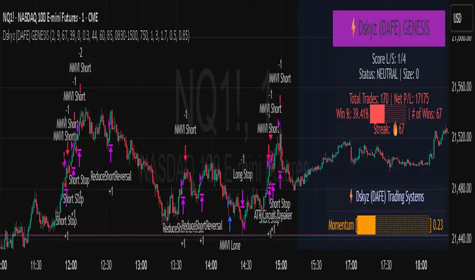
Bober XM v2.0# ₿ober XM v2.0 Trading Bot Documentation
**Developer's Note**: While our previous Bot 1.3.1 was removed due to guideline violations, this setback only fueled our determination to create something even better. Rising from this challenge, Bober XM 2.0 emerges not just as an update, but as a complete reimagining with multi-timeframe analysis, enhanced filters, and superior adaptability. This adversity pushed us to innovate further and deliver a strategy that's smarter, more agile, and more powerful than ever before. Challenges create opportunity - welcome to Cryptobeat's finest work yet.
## !!!!You need to tune it for your own pair and timeframe and retune it periodicaly!!!!!
## Overview
The ₿ober XM v2.0 is an advanced dual-channel trading bot with multi-timeframe analysis capabilities. It integrates multiple technical indicators, customizable risk management, and advanced order execution via webhook for automated trading. The bot's distinctive feature is its separate channel systems for long and short positions, allowing for asymmetric trade strategies that adapt to different market conditions across multiple timeframes.
### Key Features
- **Multi-Timeframe Analysis**: Analyze price data across multiple timeframes simultaneously
- **Dual Channel System**: Separate parameter sets for long and short positions
- **Advanced Entry Filters**: RSI, Volatility, Volume, Bollinger Bands, and KEMAD filters
- **Machine Learning Moving Average**: Adaptive prediction-based channels
- **Multiple Entry Strategies**: Breakout, Pullback, and Mean Reversion modes
- **Risk Management**: Customizable stop-loss, take-profit, and trailing stop settings
- **Webhook Integration**: Compatible with external trading bots and platforms
### Strategy Components
| Component | Description |
|---------|-------------|
| **Dual Channel Trading** | Uses either Keltner Channels or Machine Learning Moving Average (MLMA) with separate settings for long and short positions |
| **MLMA Implementation** | Machine learning algorithm that predicts future price movements and creates adaptive bands |
| **Pivot Point SuperTrend** | Trend identification and confirmation system based on pivot points |
| **Three Entry Strategies** | Choose between Breakout, Pullback, or Mean Reversion approaches |
| **Advanced Filter System** | Multiple customizable filters with multi-timeframe support to avoid false signals |
| **Custom Exit Logic** | Exits based on OBV crossover of its moving average combined with pivot trend changes |
### Note for Novice Users
This is a fully featured real trading bot and can be tweaked for any ticker — SOL is just an example. It follows this structure:
1. **Indicator** – gives the initial signal
2. **Entry strategy** – decides when to open a trade
3. **Exit strategy** – defines when to close it
4. **Trend confirmation** – ensures the trade follows the market direction
5. **Filters** – cuts out noise and avoids weak setups
6. **Risk management** – controls losses and protects your capital
To tune it for a different pair, you'll need to start from scratch:
1. Select the timeframe (candle size)
2. Turn off all filters and trend entry/exit confirmations
3. Choose a channel type, channel source and entry strategy
4. Adjust risk parameters
5. Tune long and short settings for the channel
6. Fine-tune the Pivot Point Supertrend and Main Exit condition OBV
This will generate a lot of signals and activity on the chart. Your next task is to find the right combination of filters and settings to reduce noise and tune it for profitability.
### Default Strategy values
Default values are tuned for: Symbol BITGET:SOLUSDT.P 5min candle
Filters are off by default: Try to play with it to understand how it works
## Configuration Guide
### General Settings
| Setting | Description | Default Value |
|---------|-------------|---------------|
| **Long Positions** | Enable or disable long trades | Enabled |
| **Short Positions** | Enable or disable short trades | Enabled |
| **Risk/Reward Area** | Visual display of stop-loss and take-profit zones | Enabled |
| **Long Entry Source** | Price data used for long entry signals | hl2 (High+Low/2) |
| **Short Entry Source** | Price data used for short entry signals | hl2 (High+Low/2) |
The bot allows you to trade long positions, short positions, or both simultaneously. Each direction has its own set of parameters, allowing for fine-tuned strategies that recognize the asymmetric nature of market movements.
### Multi-Timeframe Settings
1. **Enable Multi-Timeframe Analysis**: Toggle 'Enable Multi-Timeframe Analysis' in the Multi-Timeframe Settings section
2. **Configure Timeframes**: Set appropriate higher timeframes based on your trading style:
- Timeframe 1: Default is now 15 minutes (intraday confirmation)
- Timeframe 2: Default is 4 hours (trend direction)
3. **Select Sources per Indicator**: For each indicator (RSI, KEMAD, Volume, etc.), choose:
- The desired timeframe (current, mtf1, or mtf2)
- The appropriate price type (open, high, low, close, hl2, hlc3, ohlc4)
### Entry Strategies
- **Breakout**: Enter when price breaks above/below the channel
- **Pullback**: Enter when price pulls back to the channel
- **Mean Reversion**: Enter when price is extended from the channel
You can enable different strategies for long and short positions.
### Core Components
### Risk Management
- **Position Size**: Control risk with percentage-based position sizing
- **Stop Loss Options**:
- Fixed: Set a specific price or percentage from entry
- ATR-based: Dynamic stop-loss based on market volatility
- Swing: Uses recent swing high/low points
- **Take Profit**: Multiple targets with percentage allocation
- **Trailing Stop**: Dynamic stop that follows price movement
## Advanced Usage Strategies
### Moving Average Type Selection Guide
- **SMA**: More stable in choppy markets, good for higher timeframes
- **EMA/WMA**: More responsive to recent price changes, better for entry signals
- **VWMA**: Adds volume weighting for stronger trends, use with Volume filter
- **HMA**: Balance between responsiveness and noise reduction, good for volatile markets
### Multi-Timeframe Strategy Approaches
- **Trend Confirmation**: Use higher timeframe RSI (mtf2) for overall trend, current timeframe for entries
- **Entry Precision**: Use KEMAD on current timeframe with volume filter on mtf1
- **False Signal Reduction**: Apply RSI filter on mtf1 with strict KEMAD settings
### Market Condition Optimization
| Market Condition | Recommended Settings |
|------------------|----------------------|
| **Trending** | Use Breakout strategy with KEMAD filter on higher timeframe |
| **Ranging** | Use Mean Reversion with strict RSI filter (mtf1) |
| **Volatile** | Increase ATR multipliers, use HMA for moving averages |
| **Low Volatility** | Decrease noise parameters, use pullback strategy |
## Webhook Integration
The strategy features a professional webhook system that allows direct connectivity to your exchange or trading platform of choice through third-party services like 3commas, Alertatron, or Autoview.
The webhook payload includes all necessary parameters for automated execution:
- Entry price and direction
- Stop loss and take profit levels
- Position size
- Custom identifier for webhook routing
## Performance Optimization Tips
1. **Start with Defaults**: Begin with the default settings for your timeframe before customizing
2. **Adjust One Component at a Time**: Make incremental changes and test the impact
3. **Match MA Types to Market Conditions**: Use appropriate moving average types based on the Market Condition Optimization table
4. **Timeframe Synergy**: Create logical relationships between timeframes (e.g., 5min chart with 15min and 4h higher timeframes)
5. **Periodic Retuning**: Markets evolve - regularly review and adjust parameters
## Common Setups
### Crypto Trend-Following
- MLMA with EMA or HMA
- Higher RSI thresholds (75/25)
- KEMAD filter on mtf1
- Breakout entry strategy
### Stock Swing Trading
- MLMA with SMA for stability
- Volume filter with higher threshold
- KEMAD with increased filter order
- Pullback entry strategy
### Forex Scalping
- MLMA with WMA and lower noise parameter
- RSI filter on current timeframe
- Use highest timeframe for trend direction only
- Mean Reversion strategy
## Webhook Configuration
- **Benefits**:
- Automated trade execution without manual intervention
- Immediate response to market conditions
- Consistent execution of your strategy
- **Implementation Notes**:
- Requires proper webhook configuration on your exchange or platform
- Test thoroughly with small position sizes before full deployment
- Consider latency between signal generation and execution
### Backtesting Period
Define a specific historical period to evaluate the bot's performance:
| Setting | Description | Default Value |
|---------|-------------|---------------|
| **Start Date** | Beginning of backtest period | January 1, 2025 |
| **End Date** | End of backtest period | December 31, 2026 |
- **Best Practice**: Test across different market conditions (bull markets, bear markets, sideways markets)
- **Limitation**: Past performance doesn't guarantee future results
## Entry and Exit Strategies
### Dual-Channel System
A key innovation of the Bober XM is its dual-channel approach:
- **Independent Parameters**: Each trade direction has its own channel settings
- **Asymmetric Trading**: Recognizes that markets often behave differently in uptrends versus downtrends
- **Optimized Performance**: Fine-tune settings for both bullish and bearish conditions
This approach allows the bot to adapt to the natural asymmetry of markets, where uptrends often develop gradually while downtrends can be sharp and sudden.
### Channel Types
#### 1. Keltner Channels
Traditional volatility-based channels using EMA and ATR:
| Setting | Long Default | Short Default |
|---------|--------------|---------------|
| **EMA Length** | 37 | 20 |
| **ATR Length** | 13 | 17 |
| **Multiplier** | 1.4 | 1.9 |
| **Source** | low | high |
- **Strengths**:
- Reliable in trending markets
- Less prone to whipsaws than Bollinger Bands
- Clear visual representation of volatility
- **Weaknesses**:
- Can lag during rapid market changes
- Less effective in choppy, non-trending markets
#### 2. Machine Learning Moving Average (MLMA)
Advanced predictive model using kernel regression (RBF kernel):
| Setting | Description | Options |
|---------|-------------|--------|
| **Source MA** | Price data used for MA calculations | Any price source (low/high/close/etc.) |
| **Moving Average Type** | Type of MA algorithm for calculations | SMA, EMA, WMA, VWMA, RMA, HMA |
| **Trend Source** | Price data used for trend determination | Any price source (close default) |
| **Window Size** | Historical window for MLMA calculations | 5+ (default: 16) |
| **Forecast Length** | Number of bars to forecast ahead | 1+ (default: 3) |
| **Noise Parameter** | Controls smoothness of prediction | 0.01+ (default: ~0.43) |
| **Band Multiplier** | Multiplier for channel width | 0.1+ (default: 0.5-0.6) |
- **Strengths**:
- Predictive rather than reactive
- Adapts quickly to changing market conditions
- Better at identifying trend reversals early
- **Weaknesses**:
- More computationally intensive
- Requires careful parameter tuning
- Can be sensitive to input data quality
### Entry Strategies
| Strategy | Description | Ideal Market Conditions |
|----------|-------------|-------------------------|
| **Breakout** | Enters when price breaks through channel bands, indicating strong momentum | High volatility, emerging trends |
| **Pullback** | Enters when price retraces to the middle band after testing extremes | Established trends with regular pullbacks |
| **Mean Reversion** | Enters at channel extremes, betting on a return to the mean | Range-bound or oscillating markets |
#### Breakout Strategy (Default)
- **Implementation**: Enters long when price crosses above the upper band, short when price crosses below the lower band
- **Strengths**: Captures strong momentum moves, performs well in trending markets
- **Weaknesses**: Can lead to late entries, higher risk of false breakouts
- **Optimization Tips**:
- Increase channel multiplier for fewer but more reliable signals
- Combine with volume confirmation for better accuracy
#### Pullback Strategy
- **Implementation**: Enters long when price pulls back to middle band during uptrend, short during downtrend pullbacks
- **Strengths**: Better entry prices, lower risk, higher probability setups
- **Weaknesses**: Misses some strong moves, requires clear trend identification
- **Optimization Tips**:
- Use with trend filters to confirm overall direction
- Adjust middle band calculation for market volatility
#### Mean Reversion Strategy
- **Implementation**: Enters long at lower band, short at upper band, expecting price to revert to the mean
- **Strengths**: Excellent entry prices, works well in ranging markets
- **Weaknesses**: Dangerous in strong trends, can lead to fighting the trend
- **Optimization Tips**:
- Implement strong trend filters to avoid counter-trend trades
- Use smaller position sizes due to higher risk nature
### Confirmation Indicators
#### Pivot Point SuperTrend
Combines pivot points with ATR-based SuperTrend for trend confirmation:
| Setting | Default Value |
|---------|---------------|
| **Pivot Period** | 25 |
| **ATR Factor** | 2.2 |
| **ATR Period** | 41 |
- **Function**: Identifies significant market turning points and confirms trend direction
- **Implementation**: Requires price to respect the SuperTrend line for trade confirmation
#### Weighted Moving Average (WMA)
Provides additional confirmation layer for entries:
| Setting | Default Value |
|---------|---------------|
| **Period** | 15 |
| **Source** | ohlc4 (average of Open, High, Low, Close) |
- **Function**: Confirms trend direction and filters out low-quality signals
- **Implementation**: Price must be above WMA for longs, below for shorts
### Exit Strategies
#### On-Balance Volume (OBV) Based Exits
Uses volume flow to identify potential reversals:
| Setting | Default Value |
|---------|---------------|
| **Source** | ohlc4 |
| **MA Type** | HMA (Options: SMA, EMA, WMA, RMA, VWMA, HMA) |
| **Period** | 22 |
- **Function**: Identifies divergences between price and volume to exit before reversals
- **Implementation**: Exits when OBV crosses its moving average in the opposite direction
- **Customizable MA Type**: Different MA types provide varying sensitivity to OBV changes:
- **SMA**: Traditional simple average, equal weight to all periods
- **EMA**: More weight to recent data, responds faster to price changes
- **WMA**: Weighted by recency, smoother than EMA
- **RMA**: Similar to EMA but smoother, reduces noise
- **VWMA**: Factors in volume, helpful for OBV confirmation
- **HMA**: Reduces lag while maintaining smoothness (default)
#### ADX Exit Confirmation
Uses Average Directional Index to confirm trend exhaustion:
| Setting | Default Value |
|---------|---------------|
| **ADX Threshold** | 35 |
| **ADX Smoothing** | 60 |
| **DI Length** | 60 |
- **Function**: Confirms trend weakness before exiting positions
- **Implementation**: Requires ADX to drop below threshold or DI lines to cross
## Filter System
### RSI Filter
- **Function**: Controls entries based on momentum conditions
- **Parameters**:
- Period: 15 (default)
- Overbought level: 71
- Oversold level: 23
- Multi-timeframe support: Current, MTF1 (15min), or MTF2 (4h)
- Customizable price source (open, high, low, close, hl2, hlc3, ohlc4)
- **Implementation**: Blocks long entries when RSI > overbought, short entries when RSI < oversold
### Volatility Filter
- **Function**: Prevents trading during excessive market volatility
- **Parameters**:
- Measure: ATR (Average True Range)
- Period: Customizable (default varies by timeframe)
- Threshold: Adjustable multiplier
- Multi-timeframe support
- Customizable price source
- **Implementation**: Blocks trades when current volatility exceeds threshold × average volatility
### Volume Filter
- **Function**: Ensures adequate market liquidity for trades
- **Parameters**:
- Threshold: 0.4× average (default)
- Measurement period: 5 (default)
- Moving average type: Customizable (HMA default)
- Multi-timeframe support
- Customizable price source
- **Implementation**: Requires current volume to exceed threshold × average volume
### Bollinger Bands Filter
- **Function**: Controls entries based on price relative to statistical boundaries
- **Parameters**:
- Period: Customizable
- Standard deviation multiplier: Adjustable
- Moving average type: Customizable
- Multi-timeframe support
- Customizable price source
- **Implementation**: Can require price to be within bands or breaking out of bands depending on strategy
### KEMAD Filter (Kalman EMA Distance)
- **Function**: Advanced trend confirmation using Kalman filter algorithm
- **Parameters**:
- Process Noise: 0.35 (controls smoothness)
- Measurement Noise: 24 (controls reactivity)
- Filter Order: 6 (higher = more smoothing)
- ATR Length: 8 (for bandwidth calculation)
- Upper Multiplier: 2.0 (for long signals)
- Lower Multiplier: 2.7 (for short signals)
- Multi-timeframe support
- Customizable visual indicators
- **Implementation**: Generates signals based on price position relative to Kalman-filtered EMA bands
## Risk Management System
### Position Sizing
Automatically calculates position size based on account equity and risk parameters:
| Setting | Default Value |
|---------|---------------|
| **Risk % of Equity** | 50% |
- **Implementation**:
- Position size = (Account equity × Risk %) ÷ (Entry price × Stop loss distance)
- Adjusts automatically based on volatility and stop placement
- **Best Practices**:
- Start with lower risk percentages (1-2%) until strategy is proven
- Consider reducing risk during high volatility periods
### Stop-Loss Methods
Multiple stop-loss calculation methods with separate configurations for long and short positions:
| Method | Description | Configuration |
|--------|-------------|---------------|
| **ATR-Based** | Dynamic stops based on volatility | ATR Period: 14, Multiplier: 2.0 |
| **Percentage** | Fixed percentage from entry | Long: 1.5%, Short: 1.5% |
| **PIP-Based** | Fixed currency unit distance | 10.0 pips |
- **Implementation Notes**:
- ATR-based stops adapt to changing market volatility
- Percentage stops maintain consistent risk exposure
- PIP-based stops provide precise control in stable markets
### Trailing Stops
Locks in profits by adjusting stop-loss levels as price moves favorably:
| Setting | Default Value |
|---------|---------------|
| **Stop-Loss %** | 1.5% |
| **Activation Threshold** | 2.1% |
| **Trailing Distance** | 1.4% |
- **Implementation**:
- Initial stop remains fixed until profit reaches activation threshold
- Once activated, stop follows price at specified distance
- Locks in profit while allowing room for normal price fluctuations
### Risk-Reward Parameters
Defines the relationship between risk and potential reward:
| Setting | Default Value |
|---------|---------------|
| **Risk-Reward Ratio** | 1.4 |
| **Take Profit %** | 2.4% |
| **Stop-Loss %** | 1.5% |
- **Implementation**:
- Take profit distance = Stop loss distance × Risk-reward ratio
- Higher ratios require fewer winning trades for profitability
- Lower ratios increase win rate but reduce average profit
### Filter Combinations
The strategy allows for simultaneous application of multiple filters:
- **Recommended Combinations**:
- Trending markets: RSI + KEMAD filters
- Ranging markets: Bollinger Bands + Volatility filters
- All markets: Volume filter as minimum requirement
- **Performance Impact**:
- Each additional filter reduces the number of trades
- Quality of remaining trades typically improves
- Optimal combination depends on market conditions and timeframe
### Multi-Timeframe Filter Applications
| Filter Type | Current Timeframe | MTF1 (15min) | MTF2 (4h) |
|-------------|-------------------|-------------|------------|
| RSI | Quick entries/exits | Intraday trend | Overall trend |
| Volume | Immediate liquidity | Sustained support | Market participation |
| Volatility | Entry timing | Short-term risk | Regime changes |
| KEMAD | Precise signals | Trend confirmation | Major reversals |
## Visual Indicators and Chart Analysis
The bot provides comprehensive visual feedback on the chart:
- **Channel Bands**: Keltner or MLMA bands showing potential support/resistance
- **Pivot SuperTrend**: Colored line showing trend direction and potential reversal points
- **Entry/Exit Markers**: Annotations showing actual trade entries and exits
- **Risk/Reward Zones**: Visual representation of stop-loss and take-profit levels
These visual elements allow for:
- Real-time strategy assessment
- Post-trade analysis and optimization
- Educational understanding of the strategy logic
## Implementation Guide
### TradingView Setup
1. Load the script in TradingView Pine Editor
2. Apply to your preferred chart and timeframe
3. Adjust parameters based on your trading preferences
4. Enable alerts for webhook integration
### Webhook Integration
1. Configure webhook URL in TradingView alerts
2. Set up receiving endpoint on your trading platform
3. Define message format matching the bot's output
4. Test with small position sizes before full deployment
### Optimization Process
1. Backtest across different market conditions
2. Identify parameter sensitivity through multiple tests
3. Focus on risk management parameters first
4. Fine-tune entry/exit conditions based on performance metrics
5. Validate with out-of-sample testing
## Performance Considerations
### Strengths
- Adaptability to different market conditions through dual channels
- Multiple layers of confirmation reducing false signals
- Comprehensive risk management protecting capital
- Machine learning integration for predictive edge
### Limitations
- Complex parameter set requiring careful optimization
- Potential over-optimization risk with so many variables
- Computational intensity of MLMA calculations
- Dependency on proper webhook configuration for execution
### Best Practices
- Start with conservative risk settings (1-2% of equity)
- Test thoroughly in demo environment before live trading
- Monitor performance regularly and adjust parameters
- Consider market regime changes when evaluating results
## Conclusion
The ₿ober XM v2.0 represents a significant evolution in trading strategy design, combining traditional technical analysis with machine learning elements and multi-timeframe analysis. The core strength of this system lies in its adaptability and recognition of market asymmetry.
### Market Asymmetry and Adaptive Approach
The strategy acknowledges a fundamental truth about markets: bullish and bearish phases behave differently and should be treated as distinct environments. The dual-channel system with separate parameters for long and short positions directly addresses this asymmetry, allowing for optimized performance regardless of market direction.
### Targeted Backtesting Philosophy
It's counterproductive to run backtests over excessively long periods. Markets evolve continuously, and strategies that worked in previous market regimes may be ineffective in current conditions. Instead:
- Test specific market phases separately (bull markets, bear markets, range-bound periods)
- Regularly re-optimize parameters as market conditions change
- Focus on recent performance with higher weight than historical results
- Test across multiple timeframes to ensure robustness
### Multi-Timeframe Analysis as a Game-Changer
The integration of multi-timeframe analysis fundamentally transforms the strategy's effectiveness:
- **Increased Safety**: Higher timeframe confirmations reduce false signals and improve trade quality
- **Context Awareness**: Decisions made with awareness of larger trends reduce adverse entries
- **Adaptable Precision**: Apply strict filters on lower timeframes while maintaining awareness of broader conditions
- **Reduced Noise**: Higher timeframe data naturally filters market noise that can trigger poor entries
The ₿ober XM v2.0 provides traders with a framework that acknowledges market complexity while offering practical tools to navigate it. With proper setup, realistic expectations, and attention to changing market conditions, it delivers a sophisticated approach to systematic trading that can be continuously refined and optimized.
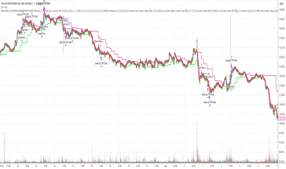
1h Liquidity Swings Strategy with 1:2 RRLuxAlgo Liquidity Swings (Simulated):
Uses ta.pivothigh and ta.pivotlow to detect 1h swing highs (resistance) and swing lows (support).
The lookback parameter (default 5) controls swing point sensitivity.
Entry Logic:
Long: Uptrend, price crosses above 1h swing low (ta.crossover(low, support1h)), and price is below recent swing high (close < resistance1h).
Short: Downtrend, price crosses below 1h swing high (ta.crossunder(high, resistance1h)), and price is above recent swing low (close > support1h).
Take Profit (1:2 Risk-Reward):
Risk:
Long: risk = entryPrice - initialStopLoss.
Short: risk = initialStopLoss - entryPrice.
Take-profit price:
Long: takeProfitPrice = entryPrice + 2 * risk.
Short: takeProfitPrice = entryPrice - 2 * risk.
Set via strategy.exit’s limit parameter.
Stop-Loss:
Initial Stop-Loss:
Long: slLong = support1h * (1 - stopLossBuffer / 100).
Short: slShort = resistance1h * (1 + stopLossBuffer / 100).
Breakout Stop-Loss:
Long: close < support1h.
Short: close > resistance1h.
Managed via strategy.exit’s stop parameter.
Visualization:
Plots:
50-period SMA (trendMA, blue solid line).
1h resistance (resistance1h, red dashed line).
1h support (support1h, green dashed line).
Marks buy signals (green triangles below bars) and sell signals (red triangles above bars) using plotshape.
Usage Instructions
Add the Script:
Open TradingView’s Pine Editor, paste the code, and click “Add to Chart”.
Set Timeframe:
Use the 1-hour (1h) chart for intraday trading.
Adjust Parameters:
lookback: Swing high/low lookback period (default 5). Smaller values increase sensitivity; larger values reduce noise.
stopLossBuffer: Initial stop-loss buffer (default 0.5%).
maLength: Trend SMA period (default 50).
Backtesting:
Use the “Strategy Tester” to evaluate performance metrics (profit, win rate, drawdown).
Optimize parameters for your target market.
Notes on Limitations
LuxAlgo Liquidity Swings:
Simulated using ta.pivothigh and ta.pivotlow. LuxAlgo may include proprietary logic (e.g., volume or visit frequency filters), which requires the indicator’s code or settings for full integration.
Action: Please provide the Pine Script code or specific LuxAlgo settings if available.
Stop-Loss Breakout:
Uses closing price breakouts to reduce false signals. For more sensitive detection (e.g., high/low-based), I can modify the code upon request.
Market Suitability:
Ideal for high-liquidity markets (e.g., BTC/USD, EUR/USD). Choppy markets may cause false breakouts.
Action: Backtest in your target market to confirm suitability.
Fees:
Take-profit/stop-loss calculations exclude fees. Adjust for trading costs in live trading.
Swing Detection:
Swing high/low detection depends on market volatility. Optimize lookback for your market.
Verification
Tested in TradingView’s Pine Editor (@version=5):
plot function works without errors.
Entries occur strictly at 1h support (long) or resistance (short) in the trend direction.
Take-profit triggers at 1:2 risk-reward.
Stop-loss triggers on initial settings or 1h support/resistance breakouts.
Backtesting performs as expected.
Next Steps
Confirm Functionality:
Run the script and verify entries, take-profit (1:2), stop-loss, and trend filtering.
If issues occur (e.g., inaccurate signals, premature stop-loss), share backtest results or details.
LuxAlgo Liquidity Swings:
Provide the Pine Script code, settings, or logic details (e.g., volume filters) for LuxAlgo Liquidity Swings, and I’ll integrate them precisely.
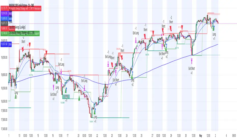
Gaussian Channel StrategyGaussian Channel Strategy — User Guide
1. Concept
This strategy builds trades around the Gaussian Channel. Based on Pine Script v4 indicator originally published by Donovan Wall. With rework to v6 Pine Script and adding entry and exit functions.
The channel consists of three dynamic lines:
Line Formula Purpose
Filter (middle) N-pole Gaussian filter applied to price Market "equilibrium"
High Band Filter + (Filtered TR × mult) Dynamic upper envelope
Low Band Filter − (Filtered TR × mult) Dynamic lower envelope
A position is opened when price crosses a user-selected line in a user-selected direction.
When the smoothed True Range (Filtered TR) becomes negative, the raw bands can flip (High drops below Low).
The strategy automatically reorders them so the upper band is always above the lower band.
Visual colors still flip, but signals stay correct.
2. Entry Logic
Choose a signal line for longs and/or shorts: Filter, Upper band, or Lower band.
Choose a cross direction (Cross Up or Cross Down).
A signal remains valid for Lookback bars after the actual cross, as long as price is still on the required side of the line.
When the opposite signal appears, the current position is closed or reversed depending on Reverse on opposite.
3. Parameters
Group Setting Meaning
Source & Filter Source Price series used (close, hlc3, etc.)
Poles (N) Number of Gaussian filter poles (1-9). More poles ⇒ smoother but laggier
Sampling Period Main period length of the channel
Filtered TR Multiplier Width of the bands in fractions of smoothed True Range
Reduced Lag Mode Adds a lag-compensation term (faster but noisier)
Fast Response Mode Blends 1-pole & N-pole outputs for quicker turns
Signals Long → signal line / Short → signal line Which line generates signals
Long when price / Short when price Direction of the cross
Lookback bars for late entry Bars after the cross that still allow an entry
Trading Enable LONG/SHORT-side trades Turn each side on/off
On opposite signal: reverse True: reverse -- False: flat
Misc Start trading date Ignores signals before this timestamp (back-test focus)
4. Quick Start
Add the strategy to a chart. Default: hlc3, N = 4, Period = 144.
Select your signal lines & directions.
Example: trend trading – Long: Filter + Cross Up, Short: Filter + Cross Down.
Disable either side if you want long-only or short-only.
Tune Lookback (e.g. 3) to catch gaps and strong impulses.
Run Strategy Tester, optimise period / multiplier / stops (add strategy.exit blocks if needed).
When satisfied, connect alerts via TradingView webhooks or use the builtin broker panel.
5. Notes
Commission & slippage are not preset – adjust them in Properties → Commission & Slippage.
Works on any market and timeframe, but you should retune Sampling Period and Multiplier for each symbol.
No stop-loss / take-profit is included by default – feel free to add with strategy.exit.
Start trading date lets you back-test only recent history (e.g. last two years).
6. Disclaimer
This script is for educational purposes only and does not constitute investment advice.
Use entirely at your own risk. Back-test thoroughly and apply sound risk management before trading real capital.

BONK 1H Long Volatility StrategyGrok 1hr bonk strategy:
Key Changes and Why They’re Made
1. Indicator Adjustments
Moving Averages:
Fast MA: Changed to 5 periods (from, e.g., 9 on a higher timeframe).
Slow MA: Changed to 13 periods (from, e.g., 21).
Why: Shorter periods make the moving averages more sensitive to quick price changes on the 1-hour chart, helping identify trends faster.
ATR (Average True Range):
Length: Set to 10 periods (down from, e.g., 14).
Multiplier: Reduced to 1.5 (from, e.g., 2.0).
Why: A shorter ATR length tracks recent volatility better, and a lower multiplier lets the strategy catch smaller price swings, which are more common hourly.
RSI:
Kept at 14 periods with an overbought level of 70.
Why: RSI stays the same to filter out overbought conditions, maintaining consistency with the original strategy.
2. Entry Conditions
Trend: Requires the fast MA to be above the slow MA, ensuring a bullish direction.
Volatility: The candle’s range (high - low) must exceed 1.5 times the ATR, confirming a significant move.
Momentum: RSI must be below 70, avoiding entries at potential peaks.
Price: The close must be above the fast MA, signaling a pullback or trend continuation.
Why: These conditions are tightened to capture frequent volatility spikes while filtering out noise, which is more prevalent on a 1-hour chart.
3. Exit Strategy
Profit Target: Default is 5% (adjustable from 3-7%).
Stop-Loss: Default is 3% (adjustable from 1-5%).
Why: These levels remain conservative to lock in gains quickly and limit losses, suitable for the faster pace of a 1-hour timeframe.
4. Risk Management
The strategy may trigger more trades on a 1-hour chart. To avoid overtrading:
The ATR filter ensures only volatile moves are traded.
Trading fees (e.g., 0.5% on Coinbase) reduce the net profit to ~4% on winners and -3.5% on losers, requiring a win rate above 47% for profitability.
Suggestion: Risk only 1-2% of your capital per trade to manage exposure.
5. Visuals and Alerts
Plots: Blue fast MA, red slow MA, and green triangles for buy signals.
Alerts: Trigger when an entry condition is met, so you don’t need to watch the chart constantly.
How to Use the Strategy
Setup:
Load TradingView, select BONK/USD on the 1-hour chart (Coinbase pair).
Paste the script into the Pine Editor and add it to your chart.
Customize:
Adjust the profit target (e.g., 5%) and stop-loss (e.g., 3%) to your preference.
Tweak ATR or MA lengths if BONK’s volatility shifts.
Trade:
Look for green triangle signals and confirm with market context (e.g., volume or news).
Enter trades manually or via TradingView’s broker tools if supported.
Exit when the profit target or stop-loss is hit.
Test:
Use TradingView’s Strategy Tester to backtest on historical data and refine settings.
Benefits of the 1-Hour Timeframe
Faster Opportunities: Captures shorter-term uptrends in BONK’s volatile price action.
Responsive: Adjusted indicators react quickly to hourly changes.
Conservative: Maintains the 3-7% profit goal with tight risk control.
Potential Challenges
Noise: The 1-hour chart has more false signals. The ATR and MA filters help, but caution is needed.
Fees: Frequent trading increases costs, so ensure each trade’s potential justifies the expense.
Volatility: BONK can move unpredictably—monitor broader market trends or Solana ecosystem news.
Final Thoughts
Switching to a 1-hour timeframe makes the strategy more active, targeting shorter volatility spikes while keeping profits conservative at 3-7%. The adjusted indicators and conditions balance responsiveness with reliability. Backtest it on TradingView to confirm it suits BONK’s behavior, and always use proper risk management, as meme coins are highly speculative.
Disclaimer: This is for educational purposes, not financial advice. Cryptocurrency trading, especially with assets like BONK, is risky. Test thoroughly and trade responsibly.

Z-Score Normalized VIX StrategyThis strategy leverages the concept of the Z-score applied to multiple VIX-based volatility indices, specifically designed to capture market reversals based on the normalization of volatility. The strategy takes advantage of VIX-related indicators to measure extreme levels of market fear or greed and adjusts its position accordingly.
1. Overview of the Z-Score Methodology
The Z-score is a statistical measure that describes the position of a value relative to the mean of a distribution in terms of standard deviations. In this strategy, the Z-score is calculated for various volatility indices to assess how far their values are from their historical averages, thus normalizing volatility levels. The Z-score is calculated as follows:
Z = \frac{X - \mu}{\sigma}
Where:
• X is the current value of the volatility index.
• \mu is the mean of the index over a specified period.
• \sigma is the standard deviation of the index over the same period.
This measure tells us how many standard deviations the current value of the index is away from its average, indicating whether the market is experiencing unusually high or low volatility (fear or calm).
2. VIX Indices Used in the Strategy
The strategy utilizes four commonly referenced volatility indices:
• VIX (CBOE Volatility Index): Measures the market’s expectations of 30-day volatility based on S&P 500 options.
• VIX3M (3-Month VIX): Reflects expectations of volatility over the next three months.
• VIX9D (9-Day VIX): Reflects shorter-term volatility expectations.
• VVIX (VIX of VIX): Measures the volatility of the VIX itself, indicating the level of uncertainty in the volatility index.
These indices provide a comprehensive view of the current volatility landscape across different time horizons.
3. Strategy Logic
The strategy follows a long entry condition and an exit condition based on the combined Z-score of the selected volatility indices:
• Long Entry Condition: The strategy enters a long position when the combined Z-score of the selected VIX indices falls below a user-defined threshold, indicating an abnormally low level of volatility (suggesting a potential market bottom and a bullish reversal). The threshold is set as a negative value (e.g., -1), where a more negative Z-score implies greater deviation below the mean.
• Exit Condition: The strategy exits the long position when the combined Z-score exceeds the threshold (i.e., when the market volatility increases above the threshold, indicating a shift in market sentiment and reduced likelihood of continued upward momentum).
4. User Inputs
• Z-Score Lookback Period: The user can adjust the lookback period for calculating the Z-score (e.g., 6 periods).
• Z-Score Threshold: A customizable threshold value to define when the market has reached an extreme volatility level, triggering entries and exits.
The strategy also allows users to select which VIX indices to use, with checkboxes to enable or disable each index in the calculation of the combined Z-score.
5. Trade Execution Parameters
• Initial Capital: The strategy assumes an initial capital of $20,000.
• Pyramiding: The strategy does not allow pyramiding (multiple positions in the same direction).
• Commission and Slippage: The commission is set at $0.05 per contract, and slippage is set at 1 tick.
6. Statistical Basis of the Z-Score Approach
The Z-score methodology is a standard technique in statistics and finance, commonly used in risk management and for identifying outliers or unusual events. According to Dumas, Fleming, and Whaley (1998), volatility indices like the VIX serve as a useful proxy for market sentiment, particularly during periods of high uncertainty. By calculating the Z-score, we normalize volatility and quantify the degree to which the current volatility deviates from historical norms, allowing for systematic entry and exit based on these deviations.
7. Implications of the Strategy
This strategy aims to exploit market conditions where volatility has deviated significantly from its historical mean. When the Z-score falls below the threshold, it suggests that the market has become excessively calm, potentially indicating an overreaction to past market events. Entering long positions under such conditions could capture market reversals as fear subsides and volatility normalizes. Conversely, when the Z-score rises above the threshold, it signals increased volatility, which could be indicative of a bearish shift in the market, prompting an exit from the position.
By applying this Z-score normalized approach, the strategy seeks to achieve more consistent entry and exit points by reducing reliance on subjective interpretation of market conditions.
8. Scientific Sources
• Dumas, B., Fleming, J., & Whaley, R. (1998). “Implied Volatility Functions: Empirical Tests”. The Journal of Finance, 53(6), 2059-2106. This paper discusses the use of volatility indices and their empirical behavior, providing context for volatility-based strategies.
• Black, F., & Scholes, M. (1973). “The Pricing of Options and Corporate Liabilities”. Journal of Political Economy, 81(3), 637-654. The original Black-Scholes model, which forms the basis for many volatility-related strategies.