Fine-tune Inputs: Gann + Laplace Smooth Volume Zone OscillatorUse this Strategy to Fine-tune inputs for the GannLSVZ0 Indicator.
Strategy allows you to fine-tune the indicator for 1 TimeFrame at a time; cross Timeframe Input fine-tuning is done manually after exporting the chart data.
I suggest using "Close all" input False when fine-tuning Inputs for 1 TimeFrame. When you export data to Excel/Numbers/GSheets I suggest using "Close all" input as True, except for the lowest TimeFrame.
MEANINGFUL DESCRIPTION:
The Volume Zone oscillator breaks up volume activity into positive and negative categories. It is positive when the current closing price is greater than the prior closing price and negative when it's lower than the prior closing price. The resulting curve plots through relative percentage levels that yield a series of buy and sell signals, depending on level and indicator direction.
The Gann Laplace Smoothed Volume Zone Oscillator GannLSVZO is a refined version of the Volume Zone Oscillator, enhanced by the implementation of the upgraded Discrete Fourier Transform, the Laplace Stieltjes Transform. Its primary function is to streamline price data and diminish market noise, thus offering a clearer and more precise reflection of price trends.
By combining the Laplace with Gann Swing Entries and with Ehler's white noise histogram, users gain a comprehensive perspective on volume-related market conditions.
HOW TO USE THE INDICATOR:
The default period is 2 but can be adjusted after backtesting. (I suggest 5 VZO length and NoiceR max length 8 as-well)
The VZO points to a positive trend when it is rising above the 0% level, and a negative trend when it is falling below the 0% level. 0% level can be adjusted in setting by adjusting VzoDifference. Oscillations rising below 0% level or falling above 0% level result in a natural trend.
HOW TO USE THE STRATEGY:
Here you fine-tune the inputs until you find a combination that works well on all Timeframes you will use when creating your Automated Trade Algorithmic Strategy. I suggest 4h, 12h, 1D, 2D, 3D, 4D, 5D, 6D, W and M.
When Indicator/Strategy returns 0 or natural trend, Strategy Closes All it's positions.
ORIGINALITY & USFULLNESS:
Personal combination of Gann swings and Laplace Stieltjes Transform of a price which results in less noise Volume Zone Oscillator.
The Laplace Stieltjes Transform is a mathematical technique that transforms discrete data from the time domain into its corresponding representation in the frequency domain. This process involves breaking down a signal into its individual frequency components, thereby exposing the amplitude and phase characteristics inherent in each frequency element.
This indicator utilizes the concept of Ehler's Universal Oscillator and displays a histogram, offering critical insights into the prevailing levels of market noise. The Ehler's Universal Oscillator is grounded in a statistical model that captures the erratic and unpredictable nature of market movements. Through the application of this principle, the histogram aids traders in pinpointing times when market volatility is either rising or subsiding.
The Gann swing strategy is developed by meomeo105, this Gann high and low algorithm forms the basis of the EMA modification.
DETAILED DESCRIPTION:
My detailed description of the indicator and use cases which I find very valuable.
What is oscillator?
Oscillators are chart indicators that can assist a trader in determining overbought or oversold conditions in ranging (non-trending) markets.
What is volume zone oscillator?
Price Zone Oscillator measures if the most recent closing price is above or below the preceding closing price.
Volume Zone Oscillator is Volume multiplied by the 1 or -1 depending on the difference of the preceding 2 close prices and smoothed with Exponential moving Average.
What does this mean?
If the VZO is above 0 and VZO is rising. We have a bullish trend. Most likely.
If the VZO is below 0 and VZO is falling. We have a bearish trend. Most likely.
Rising means that VZO on close is higher than the previous day.
Falling means that VZO on close is lower than the previous day.
What if VZO is falling above 0 line?
It means we have a high probability of a bearish trend.
Thus the indicator returns 0 and Strategy closes all it's positions when falling above 0 (or rising bellow 0) and we combine higher and lower timeframes to gauge the trend.
What is approximation and smoothing?
They are mathematical concepts for making a discrete set of numbers a
continuous curved line.
Laplace Stieltjes Transform approximation of a close price are taken from aprox library.
Key Features:
You can tailor the Indicator/Strategy to your preferences with adjustable parameters such as VZO length, noise reduction settings, and smoothing length.
Volume Zone Oscillator (VZO) shows market sentiment with the VZO, enhanced with Exponential Moving Average (EMA) smoothing for clearer trend identification.
Noise Reduction leverages Euler's White noise capabilities for effective noise reduction in the VZO, providing a cleaner and more accurate representation of market dynamics.
Choose between the traditional Fast Laplace Stieltjes Transform (FLT) and the innovative Double Discrete Fourier Transform (DTF32) soothed price series to suit your analytical needs.
Use dynamic calculation of Laplace coefficient or the static one. You may modify those inputs and Strategy entries with Gann swings.
I suggest using "Close all" input False when fine-tuning Inputs for 1 TimeFrame. When you export data to Excel/Numbers/GSheets I suggest using "Close all" input as True, except for the lowest TimeFrame. I suggest using 100% equity as your default quantity for fine-tune purposes. I have to mention that 100% equity may lead to unrealistic backtesting results. Be avare. When backtesting for trading purposes use Contracts or USDT.
Cerca negli script per "the strat"

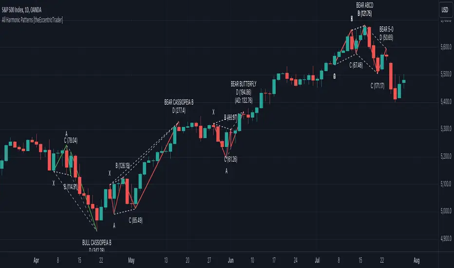
All Harmonic Patterns [theEccentricTrader]█ OVERVIEW
This indicator automatically draws and sends alerts for all of the harmonic patterns in my public library as they occur. The patterns included are as follows:
• Bearish 5-0
• Bullish 5-0
• Bearish ABCD
• Bullish ABCD
• Bearish Alternate Bat
• Bullish Alternate Bat
• Bearish Bat
• Bullish Bat
• Bearish Butterfly
• Bullish Butterfly
• Bearish Cassiopeia A
• Bullish Cassiopeia A
• Bearish Cassiopeia B
• Bullish Cassiopeia B
• Bearish Cassiopeia C
• Bullish Cassiopeia C
• Bearish Crab
• Bullish Crab
• Bearish Deep Crab
• Bullish Deep Crab
• Bearish Cypher
• Bullish Cypher
• Bearish Gartley
• Bullish Gartley
• Bearish Shark
• Bullish Shark
• Bearish Three-Drive
• Bullish Three-Drive
█ CONCEPTS
Green and Red Candles
• A green candle is one that closes with a close price equal to or above the price it opened.
• A red candle is one that closes with a close price that is lower than the price it opened.
Swing Highs and Swing Lows
• A swing high is a green candle or series of consecutive green candles followed by a single red candle to complete the swing and form the peak.
• A swing low is a red candle or series of consecutive red candles followed by a single green candle to complete the swing and form the trough.
Peak and Trough Prices
• The peak price of a complete swing high is the high price of either the red candle that completes the swing high or the high price of the preceding green candle, depending on which is higher.
• The trough price of a complete swing low is the low price of either the green candle that completes the swing low or the low price of the preceding red candle, depending on which is lower.
Historic Peaks and Troughs
The current, or most recent, peak and trough occurrences are referred to as occurrence zero. Previous peak and trough occurrences are referred to as historic and ordered numerically from right to left, with the most recent historic peak and trough occurrences being occurrence one.
Upper Trends
• A return line uptrend is formed when the current peak price is higher than the preceding peak price.
• A downtrend is formed when the current peak price is lower than the preceding peak price.
• A double-top is formed when the current peak price is equal to the preceding peak price.
Lower Trends
• An uptrend is formed when the current trough price is higher than the preceding trough price.
• A return line downtrend is formed when the current trough price is lower than the preceding trough price.
• A double-bottom is formed when the current trough price is equal to the preceding trough price.
Range
The range is simply the difference between the current peak and current trough prices, generally expressed in terms of points or pips.
Wave Cycles
A wave cycle is here defined as a complete two-part move between a swing high and a swing low, or a swing low and a swing high. The first swing high or swing low will set the course for the sequence of wave cycles that follow; for example a chart that begins with a swing low will form its first complete wave cycle upon the formation of the first complete swing high and vice versa.
Figure 1.
Retracement and Extension Ratios
Retracement and extension ratios are calculated by dividing the current range by the preceding range and multiplying the answer by 100. Retracement ratios are those that are equal to or below 100% of the preceding range and extension ratios are those that are above 100% of the preceding range.
Fibonacci Retracement and Extension Ratios
The Fibonacci sequence is a series of numbers in which each number is the sum of the two preceding numbers, starting with 0 and 1. For example 0 + 1 = 1, 1 + 1 = 2, 1 + 2 = 3, and so on. Ultimately, we could go on forever but the first few numbers in the sequence are as follows: 0 , 1, 1, 2, 3, 5, 8, 13, 21, 34, 55, 89, 144.
The extension ratios are calculated by dividing each number in the sequence by the number preceding it. For example 0/1 = 0, 1/1 = 1, 2/1 = 2, 3/2 = 1.5, 5/3 = 1.6666..., 8/5 = 1.6, 13/8 = 1.625, 21/13 = 1.6153..., 34/21 = 1.6190..., 55/34 = 1.6176..., 89/55 = 1.6181..., 144/89 = 1.6179..., and so on. The retracement ratios are calculated by inverting this process and dividing each number in the sequence by the number proceeding it. For example 0/1 = 0, 1/1 = 1, 1/2 = 0.5, 2/3 = 0.666..., 3/5 = 0.6, 5/8 = 0.625, 8/13 = 0.6153..., 13/21 = 0.6190..., 21/34 = 0.6176..., 34/55 = 0.6181..., 55/89 = 0.6179..., 89/144 = 0.6180..., and so on.
Fibonacci ranges are typically drawn from left to right, with retracement levels representing ratios inside of the current range and extension levels representing ratios extended outside of the current range. If the current wave cycle ends on a swing low, the Fibonacci range is drawn from peak to trough. If the current wave cycle ends on a swing high the Fibonacci range is drawn from trough to peak.
Measurement Tolerances
Tolerance refers to the allowable variation or deviation from a specific value or dimension. It is the range within which a particular measurement is considered to be acceptable or accurate. I have applied this concept in my pattern detection logic and have set default tolerances where applicable, as perfect patterns are, needless to say, very rare.
Chart Patterns
Generally speaking price charts are nothing more than a series of swing highs and swing lows. When demand outweighs supply over a period of time prices swing higher and when supply outweighs demand over a period of time prices swing lower. These swing highs and swing lows can form patterns that offer insight into the prevailing supply and demand dynamics at play at the relevant moment in time.
‘Let us assume… that you the reader, are not a member of that mysterious inner circle known to the boardrooms as “the insiders”… But it is fairly certain that there are not nearly so many “insiders” as amateur trader supposes and… It is even more certain that insiders can be wrong… Any success they have, however, can be accomplished only by buying and selling… hey can do neither without altering the delicate poise of supply and demand that governs prices. Whatever they do is sooner or later reflected on the charts where you… can detect it. Or detect, at least, the way in which the supply-demand equation is being affected… So, you do not need to be an insider to ride with them frequently… prices move in trends. Some of those trends are straight, some are curved; some are brief and some are long and continued… produced in a series of action and reaction waves of great uniformity. Sooner or later, these trends change direction; they may reverse (as from up to down), or they may be interrupted by some sort of sideways movement and then, after a time, proceed again in their former direction… when a price trend is in the process of reversal… a characteristic area or pattern takes shape on the chart, which becomes recognisable as a reversal formation… Needless to say, the first and most important task of the technical chart analyst is to learn to know the important reversal formations and to judge what they may signify in terms of trading opportunities’ (Edwards & Magee, 1948).
This is as true today as it was when Edwards and Magee were writing in the first half of the last Century, study your patterns and make judgements for yourself about what their implications truly are on the markets and timeframes you are interested in trading.
Over the years, traders have come to discover a multitude of chart and candlestick patterns that are supposed to pertain information on future price movements. However, it is never so clear cut in practice and patterns that where once considered to be reversal patterns are now considered to be continuation patterns and vice versa. Bullish patterns can have bearish implications and bearish patterns can have bullish implications. As such, I would highly encourage you to do your own backtesting.
There is no denying that chart patterns exist, but their implications will vary from market to market and timeframe to timeframe. So it is down to you as an individual to study them and make decisions about how they may be used in a strategic sense.
Harmonic Patterns
The concept of harmonic patterns in trading was first introduced by H.M. Gartley in his book "Profits in the Stock Market", published in 1935. Gartley observed that markets have a tendency to move in repetitive patterns, and he identified several specific patterns that he believed could be used to predict future price movements. The bullish and bearish Gartley patterns are the oldest recognized harmonic patterns in trading and all the other harmonic patterns are modifications of the original Gartley patterns. Gartley patterns are fundamentally composed of 5 points, or 4 waves.
Since then, many other traders and analysts have built upon Gartley's work and developed their own variations of harmonic patterns. One such contributor is Larry Pesavento, who developed his own methods for measuring harmonic patterns using Fibonacci ratios. Pesavento has written several books on the subject of harmonic patterns and Fibonacci ratios in trading. Another notable contributor to harmonic patterns is Scott Carney, who developed his own approach to harmonic trading in the late 1990s and also popularised the use of Fibonacci ratios to measure harmonic patterns. Carney expanded on Gartley's work and also introduced several new harmonic patterns, such as the Shark pattern and the 5-0 pattern.
█ INPUTS
• Change pattern and label colours
• Show or hide patterns individually
• Adjust pattern tolerances
• Set or remove alerts for individual patterns
█ NOTES
You can test the patterns with your own strategies manually by applying the indicator to your chart while in bar replay mode and playing through the history. You could also automate this process with PineScript by using the conditions from my swing and pattern libraries as entry conditions in the strategy tester or your own custom made strategy screener.
█ LIMITATIONS
All green and red candle calculations are based on differences between open and close prices, as such I have made no attempt to account for green candles that gap lower and close below the close price of the preceding candle, or red candles that gap higher and close above the close price of the preceding candle. This may cause some unexpected behaviour on some markets and timeframes. I can only recommend using 24-hour markets, if and where possible, as there are far fewer gaps and, generally, more data to work with.
█ SOURCES
Edwards, R., & Magee, J. (1948) Technical Analysis of Stock Trends (10th edn). Reprint, Boca Raton, Florida: Taylor and Francis Group, CRC Press: 2013.
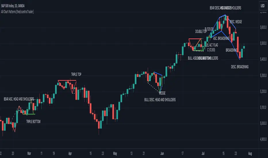
All Chart Patterns [theEccentricTrader]█ OVERVIEW
This indicator automatically draws and sends alerts for all of the chart patterns in my public library as they occur. The patterns included are as follows:
• Ascending Broadening
• Broadening
• Descending Broadening
• Double Bottom
• Double Top
• Triple Bottom
• Triple Top
• Bearish Elliot Wave
• Bullish Elliot Wave
• Bearish Alternate Flag
• Bullish Alternate Flag
• Bearish Flag
• Bullish Flag
• Bearish Ascending Head and Shoulders
• Bullish Ascending Head and Shoulders
• Bearish Descending Head and Shoulders
• Bullish Descending Head and Shoulders
• Bearish Head and Shoulders
• Bullish Head and Shoulders
• Bearish Pennant
• Bullish Pennant
• Ascending Wedge
• Descending Wedge
• Wedge
█ CONCEPTS
Green and Red Candles
• A green candle is one that closes with a close price equal to or above the price it opened.
• A red candle is one that closes with a close price that is lower than the price it opened.
Swing Highs and Swing Lows
• A swing high is a green candle or series of consecutive green candles followed by a single red candle to complete the swing and form the peak.
• A swing low is a red candle or series of consecutive red candles followed by a single green candle to complete the swing and form the trough.
Peak and Trough Prices
• The peak price of a complete swing high is the high price of either the red candle that completes the swing high or the high price of the preceding green candle, depending on which is higher.
• The trough price of a complete swing low is the low price of either the green candle that completes the swing low or the low price of the preceding red candle, depending on which is lower.
Historic Peaks and Troughs
The current, or most recent, peak and trough occurrences are referred to as occurrence zero. Previous peak and trough occurrences are referred to as historic and ordered numerically from right to left, with the most recent historic peak and trough occurrences being occurrence one.
Upper Trends
• A return line uptrend is formed when the current peak price is higher than the preceding peak price.
• A downtrend is formed when the current peak price is lower than the preceding peak price.
• A double-top is formed when the current peak price is equal to the preceding peak price.
Lower Trends
• An uptrend is formed when the current trough price is higher than the preceding trough price.
• A return line downtrend is formed when the current trough price is lower than the preceding trough price.
• A double-bottom is formed when the current trough price is equal to the preceding trough price.
Range
The range is simply the difference between the current peak and current trough prices, generally expressed in terms of points or pips.
Retracement and Extension Ratios
Retracement and extension ratios are calculated by dividing the current range by the preceding range and multiplying the answer by 100. Retracement ratios are those that are equal to or below 100% of the preceding range and extension ratios are those that are above 100% of the preceding range.
Measurement Tolerances
Tolerance refers to the allowable variation or deviation from a specific value or dimension. It is the range within which a particular measurement is considered to be acceptable or accurate. I have applied this concept in my pattern detection logic and have set default tolerances where applicable, as perfect patterns are, needless to say, very rare.
Chart Patterns
Generally speaking price charts are nothing more than a series of swing highs and swing lows. When demand outweighs supply over a period of time prices swing higher and when supply outweighs demand over a period of time prices swing lower. These swing highs and swing lows can form patterns that offer insight into the prevailing supply and demand dynamics at play at the relevant moment in time.
‘Let us assume… that you the reader, are not a member of that mysterious inner circle known to the boardrooms as “the insiders”… But it is fairly certain that there are not nearly so many “insiders” as amateur trader supposes and… It is even more certain that insiders can be wrong… Any success they have, however, can be accomplished only by buying and selling… hey can do neither without altering the delicate poise of supply and demand that governs prices. Whatever they do is sooner or later reflected on the charts where you… can detect it. Or detect, at least, the way in which the supply-demand equation is being affected… So, you do not need to be an insider to ride with them frequently… prices move in trends. Some of those trends are straight, some are curved; some are brief and some are long and continued… produced in a series of action and reaction waves of great uniformity. Sooner or later, these trends change direction; they may reverse (as from up to down), or they may be interrupted by some sort of sideways movement and then, after a time, proceed again in their former direction… when a price trend is in the process of reversal… a characteristic area or pattern takes shape on the chart, which becomes recognisable as a reversal formation… Needless to say, the first and most important task of the technical chart analyst is to learn to know the important reversal formations and to judge what they may signify in terms of trading opportunities’ (Edwards & Magee, 1948).
This is as true today as it was when Edwards and Magee were writing in the first half of the last Century, study your patterns and make judgements for yourself about what their implications truly are on the markets and timeframes you are interested in trading.
Over the years, traders have come to discover a multitude of chart and candlestick patterns that are supposed to pertain information on future price movements. However, it is never so clear cut in practice and patterns that where once considered to be reversal patterns are now considered to be continuation patterns and vice versa. Bullish patterns can have bearish implications and bearish patterns can have bullish implications. As such, I would highly encourage you to do your own backtesting.
There is no denying that chart patterns exist, but their implications will vary from market to market and timeframe to timeframe. So it is down to you as an individual to study them and make decisions about how they may be used in a strategic sense.
█ INPUTS
• Change pattern and label colours
• Show or hide patterns individually
• Adjust pattern ratios and tolerances
• Set or remove alerts for individual patterns
█ NOTES
I have decided to rename some of my previously published patterns based on the way in which the pattern completes. If the pattern completes on a swing high then the pattern is considered bearish, if the pattern completes on a swing low then it is considered bullish. This may seem confusing but it makes sense when you come to backtesting the patterns and want to use the most recent peak or trough prices as stop losses. Patterns that can complete on both a swing high and swing low are for such reasons treated as neutral, namely all broadening and wedge variations. I trust that it is quite self-evident that double and triple bottom patterns are considered bullish while double and triple top patterns are considered bearish, so I did not feel the need to rename those.
The patterns that have been renamed and what they have been renamed to, are as follows:
• Ascending Elliot Waves to Bearish Elliot Waves
• Descending Elliot Waves to Bullish Elliot Waves
• Ascending Head and Shoulders to Bearish Ascending Head and Shoulders
• Descending Head and Shoulders to Bearish Descending Head and Shoulders
• Head and Shoulders to Bearish Head and Shoulders
• Ascending Inverse Head and Shoulders to Bullish Ascending Head and Shoulders
• Descending Inverse Head and Shoulders to Bullish Descending Head and Shoulders
• Inverse Head and Shoulders to Bullish Head and Shoulders
You can test the patterns with your own strategies manually by applying the indicator to your chart while in bar replay mode and playing through the history. You could also automate this process with PineScript by using the conditions from my swing and pattern libraries as entry conditions in the strategy tester or your own custom made strategy screener.
█ LIMITATIONS
All green and red candle calculations are based on differences between open and close prices, as such I have made no attempt to account for green candles that gap lower and close below the close price of the preceding candle, or red candles that gap higher and close above the close price of the preceding candle. This may cause some unexpected behaviour on some markets and timeframes. I can only recommend using 24-hour markets, if and where possible, as there are far fewer gaps and, generally, more data to work with.
█ SOURCES
Edwards, R., & Magee, J. (1948) Technical Analysis of Stock Trends (10th edn). Reprint, Boca Raton, Florida: Taylor and Francis Group, CRC Press: 2013.
Moving Average Crossover Swing StrategyMoving Average Crossover Swing Strategy
**Overview:**
The basic concept of this strategy is to generate a signal when a faster/shorter length moving average crosses over (for Longs) or crosses under (for Shorts) a medium/longer length moving average. All of which are customizable. This strategy can work on any timeframe, however the daily is the timeframe used for the default settings and screenshots, as it was designed to be a multi-day swing strategy. Once a signal has been confirmed with a candle close, based on user options, the strategy will enter the trade on the open of the next candle.
The crossover strategy is nothing new to trading, but what can make this strategy unique and helpful, is the addition of further confirmation points, ATR based stop loss and take profit targets, optional early exit criteria, customizable to your needs and style, and just about everything visual can be toggled on/off. This strategy is based on a Trend (MA) indicator and a Momentum (MACD) indicator. While a Volume-based indicator is not shown here, one could consider using their favorite from that category to further compliment the signal idea.
It should be noted that depending on the time frame, direction(s) chosen, the signal options, confirmation options, and exit options selected, that a ticker may not produce more than 100 trades on the back test. Depending on your style and frequency, one could consider adjusting options and/or testing multiple tickers. It should also be noted that this strategy simply tests the underlying stock prices, not options contracts. And of course, testing this strategy against historical data does not assume that the same results will occur in future price action.
Shoutout given to Ripster's Clouds Indicator as pieces of that code were taken and modified to create both the Cloud visualization effects, and the Moving Average Pair Plots that are implemented in this strategy.
BASIC DEFAULTS
All can be changed as normal
Initial capital = 10,000
Order Sizing = 25% of equity (use the "Inputs" tab to modify this)
Pyramiding = 0
Commission = 0.65 USD per order
Price Verification = 1 tick
Slippage = 1 tick
RISK MANAGMENT
You will notice two different percentage options and ATR multipliers. This strategy will adjust position sizing by not exceeding either one of those % values based on the ATR (Average True Range) of the symbol and the multipliers selected, should the stock hit the stop loss price.
For Example, lets assume these values are true:
Account size = $10,000,
Max Risk = 1% of account size
Max Position Size = 25% of the account size
Stock Price = 23.45
ATR = 3.5
ATR Stop Loss Multiplier = 1.4
Then the formulas would be:
ACCT_SIZE * MaxRisk_% = 10000 * .01 = $100 (MaxCashRisk)
-----
MaxCashRisk / (ATR * ATR_SL_MULTIPLIER) = 100 / (3.5 * 1.4) = 20.4 Shares based on Max Cash Risk
-----
(ACCT_SIZE * MaxEquity_%) / STOCK_PRICE = (10000 * .25) / 23.45 = 106.61 Shares based on Max Equity Allocation
The minimum value of each of those options is then used, which in this case would be to purchase 20 shares so as not to exceed the max dollar risk should the stock reach the stop loss target. Likewise, if the ATR were to be much lower, say 0.48 cents, and all else the same, then the strategy would purchase the 106 shares based on Max Equity Allocation because the Max Cash Risk would require 149.25 shares.
MOVING AVERAGE OPTIONS
Select between and change the length & type of up to 5 pairs (10 total) of moving averages
The "Show Cloud-x" option will display a fill color between the "a" and "b" pairs
All moving averages lines can be toggled on/off in the "Style" tab, as well as adjusting their colors.
Visualization features do not affect calculations, meaning you could have all or nothing on the chart and the strategy will still produce results
SIGNAL CHOICES
Choose the fast/shorter length MA and the medium/longer length MA to determine the entry signal
CONFIRMATION OPTIONS
Both of these have customizable values and can be toggled on/off
A candle close over a slower/much longer length moving average
An additional cross-over (cross-under for Shorts) on the MACD indicator using default MACD values. While the MACD indicator is not necessary to have on the chart, it can help to add that for visualization. The calculations will perform whether the indicator is on the chart or not.
EARLY EXIT CRITERIA
Both can be toggled on/off with customizable values
MA Cross Exit will exit the trade early if the select moving averages cross-under (for longs) or cross-over (for shorts), indicating a potential reversal.
Max Bars in Trades will act as a last-resort exit by simply calculating the amount of full bars the trade has been open, and exiting on the opening of the next bar. For example: the default value is 8 bars, so after 8 full bars in the trade, if no other exit has been triggered (Stop Loss, Take Profit, or MA Cross(if enabled)), then the trade will exit at the opening of the 9th bar.
Finally, there is a table displaying the amount of trades taken for each side, and the amount & percent of both early exits. This table can be turned off in the "Style" tab
ADDITIONAL PLOTS
MACD (Moving Average Convergence/Divergence):
- The MACD is an optional confirmation indicator for this strategy.
- Plotting the indicator is not necessary for the strategy to work, but it can be helpful to visually see the status and position of the MACD if this feature is enabled in the strategy
- This helps to identify if there is also momentum behind the entry signal

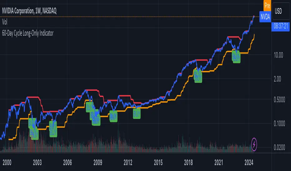
60-Day Cycle Long-Only IndicatorThe following indicator generates ‘Buy’ signals based on rotating 60-day cycles. The general theory is that when buying strong, growth-oriented assets, 60-day micro-cycles culminate into larger macro-cycles.
Summary:
Explaining the Upper and Lower Bounds in the 60-Day Cycle Strategy:
1. Cycle High (Upper Bound):
The cycle high is the highest closing price of the asset over the past 60 days. This value acts as the upper boundary of the 60-day cycle, indicating the peak price level during this period. When the current closing price is above this boundary, it suggests a potential distribution phase, where the asset might be overbought, and larger players may be selling off their positions. In the strategy, the cycle high is plotted as a red line on the chart, helping traders visually identify the upper limit of the 60-day trading range.
2. Cycle Low (Lower Bound):
The cycle low is the lowest closing price of the asset over the past 60 days. This value acts as the lower boundary of the 60-day cycle, indicating the trough price level during this period. When the current closing price is below this boundary, it suggests a potential accumulation phase, where the asset might be oversold, and larger players may be accumulating positions at lower prices. In the strategy, the cycle low is plotted as an orange line on the chart, helping traders visually identify the lower limit of the 60-day trading range.
How These Bounds Are Calculated:
• Cycle High: Calculated using the highest closing price over the last 60 trading days. In Pine Script, this is achieved with the function ta.highest(close, cycle_length), where cycle_length is set to 60 days.
• Cycle Low: Calculated using the lowest closing price over the last 60 trading days. In Pine Script, this is achieved with the function ta.lowest(close, cycle_length), where cycle_length is set to 60 days.
Interpretation and Application:
• Buy Signal: A buy signal is generated when the closing price crosses above the cycle low. This indicates a potential end to the bearish phase and the start of a bullish trend.
• Distribution Phase: When the closing price crosses above the cycle high, it suggests the market is in a distribution phase, potentially signaling a bearish trend or a sell-off period.
Example:
On a trading chart, the cycle high and cycle low are plotted as horizontal lines, with their colors distinguishing them (red for cycle high and orange for cycle low). These lines create a visual range within which the asset's price has moved over the last 60 days, helping traders quickly assess whether the current price is near the upper or lower bound.
By identifying and plotting these upper and lower bounds, traders can better understand the current market phase and make more informed trading decisions based on the 60-day cycle strategy. This indicator can be used across various assets.
TSI w SuperTrend decision - Strategy [presentTrading]This strategy aims to improve upon the performance of Traidngview's newly published "Trend Strength Index" indicator by incorporating the SuperTrend for better trade execution and risk management. Enjoy :)
█ Introduction and How it is Different
The "TSI with SuperTrend Decision - Strategy" combines the Trend Strength Index (TSI) with SuperTrend indicators to determine entry and exit points. Unlike traditional strategies that rely solely on one indicator, this method leverages the strengths of both TSI and SuperTrend to provide a more nuanced and adaptive trading strategy.
This dual approach allows for capturing trends more effectively, especially in volatile markets.
BTCUSD 8h LS Performance
█ Strategy, How it Works: Detailed Explanation
🔶 Trend Strength Index (TSI)
The TSI is a momentum oscillator that shows both the direction and strength of a trend. It is calculated by comparing the price movement with the bar index over a specified period. The formula for TSI is as follows:
```
TSI = (PC / |PC|)
where:
PC = Change in price over the period
```
In this strategy, TSI is calculated using the closing prices and a default period of 64 bars. The TSI values help identify overbought and oversold conditions, providing signals for potential market reversals.
🔶 SuperTrend Indicator
The SuperTrend is a trend-following indicator based on the average true range (ATR). It helps in identifying the direction of the market trend. The SuperTrend calculation involves:
```
SuperTrend = HLC3 ± (Factor * ATR)
where:
HLC3 = (High + Low + Close) / 3
Factor = User-defined multiplier
ATR = Average True Range over a period
```
The SuperTrend settings in this strategy include a length of 10 bars and a factor of 3.0.
Last Bull Cycle of BTC
🔶 Entry and Exit Conditions
The strategy uses the TSI and SuperTrend together to determine entry and exit points:
- Long Entry: When the SuperTrend indicates a downward trend (st.d < 0) and the TSI is above the oversold level (-0.241).
- Long Exit: When the SuperTrend indicates an upward trend (st.d > 0) and the TSI is below the overbought level (0.241).
- Short Entry: When the SuperTrend indicates an upward trend (st.d > 0) and the TSI is below the overbought level (0.241).
- Short Exit: When the SuperTrend indicates a downward trend (st.d < 0) and the TSI is above the oversold level (-0.241).
█ Trade Direction
The strategy allows users to select the trade direction through the `tradeDirection` input. The options are:
- Both: Enables both long and short trades.
- Long: Enables only long trades.
- Short: Enables only short trades.
█ Default Settings
- TSI Length: 64
- SuperTrend Length: 10
- SuperTrend Factor: 3.0
- Trade Direction: Both
- Take Profit (%): 30.0
- Stop Loss (%): 20.0
Impact of Default Settings
- TSI Length: A longer TSI period smooths out noise but may lag in identifying trends. A shorter period is more responsive but can generate false signals.
- SuperTrend Length: A shorter length provides quicker signals but can be prone to whipsaws. A longer length is more reliable but may delay entries and exits.
- SuperTrend Factor: A higher factor increases the distance of the SuperTrend from the price, reducing sensitivity to minor price fluctuations.
- Trade Direction: Allows flexibility in trading strategies by enabling both long and short trades based on market conditions.
- Take Profit and Stop Loss: These settings manage risk by automatically closing trades at predefined profit or loss levels. Higher percentages provide larger potential gains but also higher risk.

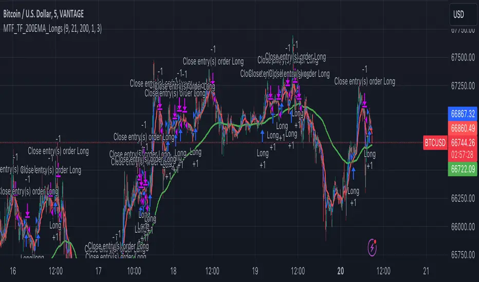
Multi-Timeframe Trend Following with 200 EMA Filter - Longs OnlyOverview
This strategy is designed to trade long positions based on multiple timeframe Exponential Moving Averages (EMAs) and a 200 EMA filter. The strategy ensures that trades are only entered in strong uptrends and aims to capitalize on sustained upward movements while minimizing risk with a defined stop-loss and take-profit mechanism.
Key Components
Initial Capital and Position Sizing
Initial Capital: $1000.
Lot Size: 1 unit per trade.
Inputs
Fast EMA Length (fast_length): The period for the fast EMA.
Slow EMA Length (slow_length): The period for the slow EMA.
200 EMA Length (filter_length_200): Set to 200 periods for the primary trend filter.
Stop Loss Percentage (stop_loss_perc): Set to 1% of the entry price.
Take Profit Percentage (take_profit_perc): Set to 3% of the entry price.
Timeframes and EMAs
EMAs are calculated for the following timeframes using the request.security function:
5-minute: Short-term trend detection.
15-minute: Intermediate-term trend detection.
30-minute: Long-term trend detection.
The strategy also calculates a 200-period EMA on the 5-minute timeframe to serve as a primary trend filter.
Trend Calculation
The strategy determines the trend for each timeframe by comparing the fast and slow EMAs:
If the fast EMA is above the slow EMA, the trend is considered positive (1).
If the fast EMA is below the slow EMA, the trend is considered negative (-1).
Combined Trend Signal
The combined trend signal is derived by summing the individual trends from the 5-minute, 15-minute, and 30-minute timeframes.
A combined trend value of 3 indicates a strong uptrend across all timeframes.
Any combined trend value less than 3 indicates a weakening or negative trend.
Entry and Exit Conditions
Entry Condition:
A long position is entered if:
The combined trend signal is 3 (indicating a strong uptrend across all timeframes).
The current close price is above the 200 EMA on the 5-minute timeframe.
Exit Condition:
The long position is exited if:
The combined trend signal is less than 3 (indicating a weakening trend).
The current close price falls below the 200 EMA on the 5-minute timeframe.
Stop Loss and Take Profit
Stop Loss: Set at 1% below the entry price.
Take Profit: Set at 3% above the entry price.
These levels are automatically set when entering a trade using the strategy.entry function with stop and limit parameters.
Plotting
The strategy plots the fast and slow EMAs for the 5-minute timeframe and the 200 EMA for visual reference on the chart:
Fast EMA (5-min): Plotted in blue.
Slow EMA (5-min): Plotted in red.
200 EMA (5-min): Plotted in green.
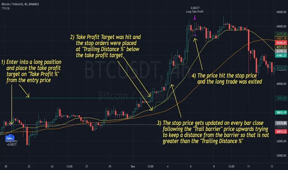
Trailing Take Profit - Close Based📝 Description
This script demonstrates a new approach to the trailing take profit.
Trailing Take Profit is a price-following technique. When used, instead of setting a limit order for the take profit target exiting from your position at the specified price, a stop order is conditionally set when the take profit target is reached. Then, the stop price (a.k.a trailing price), is placed below the take profit target at a distance defined by the user percentagewise. On regular time intervals, the stop price gets updated by following the "Trail Barrier" price (high by default) upwards. When the current price hits the stop price you exit the trade. Check the chart for more details.
This script demonstrates how to implement the close-based Trailing Take Profit logic for long positions, but it can also be applied for short positions if the logic is "reversed".
📢 NOTE
To generate some entries and showcase the "Trailing Take Profit" technique, this script uses the crossing of two moving averages. Please keep in mind that you should not relate the Backtesting results you see in the "Strategy Tester" tab with the success of the technique itself.
This is not a complete strategy per se, and the backtest results are affected by many parameters that are outside of the scope of this publication. If you choose to use this new approach of the "Trailing Take Profit" in your logic you have to make sure that you are backtesting the whole strategy.
⚔️ Comparison
In contrast to my older "Trailing Take Profit" publication where the trailing take profit implementation was tick-based, this new approach is close-based, meaning that the update of the stop price occurs at the bar close instead of every tick.
While comparing the real-time results of the two implementations is like comparing apples to oranges, because they have different dynamic behavior, the new approach offers better consistency between the backtesting results and the real-time results.
By updating the stop price on every bar close, you do not rely on the backtester assumptions anymore (check the Reasoning section below for more info).
The new approach resembles the conditional "Trailing Exit" technique, where the condition is true when the current price crosses over the take profit target. Then, the stop order is placed at the trailing price and it gets updated on every bar close to "follow" the barrier price (high). On the other hand, the older tick-based approach had more "tight" dynamics since the trailing price gets updated on every tick leaving less room for price fluctuations by making it more probable to reach the trailing price.
🤔 Reasoning
This new close-based approach addresses several practical issues the older tick-based approach had. Those issues arise mainly from the technicalities of the TV Backtester. More specifically, due to the assumptions the Broker Emulator makes for the price action of the history bars, the backtesting results in the TV Backtester are exaggerated, and depending on the timeframe, the backtesting results look way better than they are in reality.
The effect above, and the inability to reason about the performance of a strategy separated people into two groups. Those who never use this feature, because they couldn't know for sure the actual effect it might have in their strategy, (even if it turned out to be more profitable) and those who abused this type of "repainting" behavior to show off, and hijack some boosts from the community by boasting about the "fake" results of their strategies.
Even if there are ways to evaluate the effectiveness of the tick-based approach that is applied in an existing strategy (this is out of the topic of this publication), it requires extra effort to do the analysis. Using this closed-based approach we can have more predictable results, without surprises.
⚠️ Caveats
Since this approach updates the trailing price on bar close, you must wait for at least one bar to close after the price crosses over the take profit target.
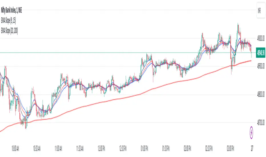
EMA Scalping StrategyEMA Slope Indicator Overview:
The indicator plots two exponential moving averages (EMAs) on the chart: a 9-period EMA and a 15-period EMA.
It visually represents the EMAs on the chart and highlights instances where the slope of each EMA exceeds a certain threshold (approximately 30 degrees).
Scalping Strategy:
Using the EMA Slope Indicator on a 5-minute timeframe for scalping can be effective, but it requires adjustments to account for the shorter time horizon.
Trend Identification: Look for instances where the 9-period EMA is above the 15-period EMA. This indicates an uptrend. Conversely, if the 9-period EMA is below the 15-period EMA, it suggests a downtrend.
Slope Analysis: Pay attention to the slope of each EMA. When the slope of both EMAs is steep (exceeds 30 degrees), it signals a strong trend. This can be a favorable condition for scalping as it suggests potential momentum.
Entry Points:
For Long (Buy) Positions: Consider entering a long position when both EMAs are sloping upwards strongly (exceeding 30 degrees) and the 9-period EMA is above the 15-period EMA. Look for entry points when price retraces to the EMAs or when there's a bullish candlestick pattern.
For Short (Sell) Positions: Look for opportunities to enter short positions when both EMAs are sloping downwards strongly (exceeding -30 degrees) and the 9-period EMA is below the 15-period EMA. Similar to long positions, consider entering on retracements or bearish candlestick patterns.
Exit Strategy: Use tight stop-loss orders to manage risk, and aim for small, quick profits. Since scalping involves short-term trading, consider exiting positions when the momentum starts to weaken or when the price reaches a predetermined profit target.
Risk Management:
Scalping involves high-frequency trading with smaller profit targets, so it's crucial to implement strict risk management practices. This includes setting stop-loss orders to limit potential losses and not risking more than a small percentage of your trading capital on each trade.
Backtesting and Optimization:
Before implementing the strategy in live trading, backtest it on historical data to assess its performance under various market conditions. You may also consider optimizing the strategy parameters (e.g., EMA lengths) to maximize its effectiveness.
Continuous Monitoring:
Keep a close eye on market conditions and adjust your strategy accordingly. Market dynamics can change rapidly, so adaptability is key to successful scalping.
Vegas SuperTrend Enhanced - Strategy [presentTrading]█ Introduction and How it is Different
The "Vegas SuperTrend Enhanced - Strategy " trading strategy represents a novel integration of two powerful technical analysis tools: the Vegas Channel and the SuperTrend indicator. This fusion creates a dynamic, adaptable strategy designed for the volatile and fast-paced cryptocurrency markets, particularly focusing on Bitcoin trading.
Unlike traditional trading strategies that rely on a static set of rules, this approach modifies the SuperTrend's sensitivity to market volatility, offering traders the ability to customize their strategy based on current market conditions. This adaptability makes it uniquely suited to navigating the often unpredictable swings in cryptocurrency valuations, providing traders with signals that are both timely and reflective of underlying market dynamics.
BTC 6h LS
█ Strategy, How it Works: Detailed Explanation
This is an innovative approach that combines the volatility-based Vegas Channel with the trend-following SuperTrend indicator to create dynamic trading signals. This section delves deeper into the mechanics and mathematical foundations of the strategy.
Detail picture to show :
🔶 Vegas Channel Calculation
The Vegas Channel serves as the foundation of this strategy, employing a simple moving average (SMA) coupled with standard deviation to define the upper and lower bounds of the trading channel. This channel adapts to price movements, offering a visual representation of potential support and resistance levels based on historical price volatility.
🔶 SuperTrend Indicator Adjustment
Central to the strategy is the SuperTrend indicator, which is adjusted according to the width of the Vegas Channel. This adjustment is achieved by modifying the SuperTrend's multiplier based on the channel's volatility, allowing the indicator to become more sensitive during periods of high volatility and less so during quieter market phases.
🔶 Trend Determination and Signal Generation
The market trend is determined by comparing the current price with the SuperTrend values. A shift from below to above the SuperTrend line signals a potential bullish trend, prompting a "buy" signal, whereas a move from above to below indicates a bearish trend, generating a "sell" signal. This methodology ensures that trades are entered in alignment with the prevailing market direction, enhancing the potential for profitability.
BTC 6h Local
█ Trade Direction
A distinctive feature of this strategy is its configurable trade direction input, allowing traders to specify whether they wish to engage in long positions, short positions, or both. This flexibility enables users to tailor the strategy according to their risk tolerance, trading style, and market outlook, providing a personalized trading experience.
█ Usage
To utilize the "Vegas SuperTrend - Enhanced" strategy effectively, traders should first adjust the input settings to align with their trading preferences and the specific characteristics of the asset being traded. Monitoring the strategy's signals within the context of overall market conditions and combining its insights with other forms of analysis can further enhance its effectiveness.
█ Default Settings
- Trade Direction: Both (allows trading in both directions)
- ATR Period for SuperTrend: 10 (determines the length of the ATR for volatility measurement)
- Vegas Window Length: 100 (sets the length of the SMA for the Vegas Channel)
- SuperTrend Multiplier Base: 5 (base multiplier for SuperTrend calculation)
- Volatility Adjustment Factor: 5.0 (adjusts SuperTrend sensitivity based on Vegas Channel width)
These default settings provide a balanced approach suitable for various market conditions but can be adjusted to meet individual trading needs and objectives.

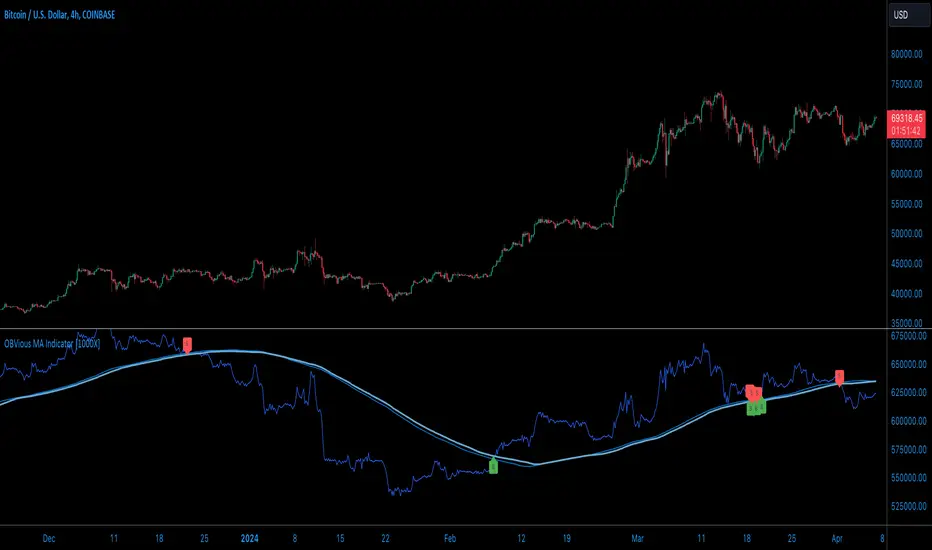
OBVious MA Indicator [1000X] On Balance Volume (OBV) is a gift to traders. OBV often provides a leading signal at the outset of a trend, when compression in the markets produces a surge in OBV prior to increased volatility.
This indicator demonstrates one method of utilizing OBV to your advantage. I call it the "OBVious MA Indicator ” only because it is simple in its mechanics. The primary utility of the OBVious MA indicator is as a volume confirmation filter that complements other components of a strategy.
Indicator Features:
• The Indicator revolves around the On Balance Volume indicator. OBV is a straightforward indicator: it registers a value by adding total volume traded on up candles, and subtracts total volume on down candles, generating a line by connecting those values. OBV was described in 1963 by Joe Granville in his book "Granville's New Key to Stock Market Profits” in which the author argues that OBV is the most vital key to success as a trader, with volume changes are a major predictor of price changes.
• Dual Moving Averages: here we use separate moving averages for entries and exits. This allows for more granular trade management; for example, one can either extend the length of the exit MA to hold positions longer, or shorten the MA for swifter exits, independently of the entry signals.
Execution: long trades are signalled when the OBV line crosses above the Long Entry Moving Average of the OBV. Long exits signals occur when the OBV line crosses under the Long Exit MA of the OBV. Shorts signal occur on a cross below the Short Entry MA, and exit signals come on a cross above the Short Exit MA.
Application:
While this indicator outlines entry and exit conditions based on OBV crossovers with designated moving averages, is is, as stated, best used in conjunction with a supporting cast of confirmatory indicators (feel free to drop me a note and tell me how you've used it). It can be used to confirm entries, or you might try using it as a sole exit indicator in a strategy.
Visualization:
The indicator includes conditional plotting of the OBV MAs, which plot based on the selected trading direction. This visualization aids in understanding how OBV interacts with the set moving averages.
Further Discussion:
We all know the importance of volume; this indicator demonstrates one simple yet effective method of incorporating the OBV for volume analysis. The OBV indicator can be used in many ways - for example, we can monitor OBV trend line breaks, look for divergences, or as we do here, watch for breaks of the moving average.
Despite its simplicity, I'm unaware of any previously published cases of this method. But the concept of applying MAs or EMAs to volume-based indicators like OBV is not uncommon in technical analysisIf, so I expect work like this has been done before. If you know of other similar indicators or strategies, please mention in the comments.
One comparable method uses EMAs of the OBV is QuantNomad’s "On Balance Volume Oscillator Strategy ”. That strategy uses a pair of EMAs on a normalized-range OBV-based oscillator. In that strategy, however, entry and exit signals occur on one EMA crossing the other, which places trades at distinctly different times than crossings of the OBV itself. Both are valid approaches with strength in simplicity.
Note: This is the indicator version of the Strategy found here .
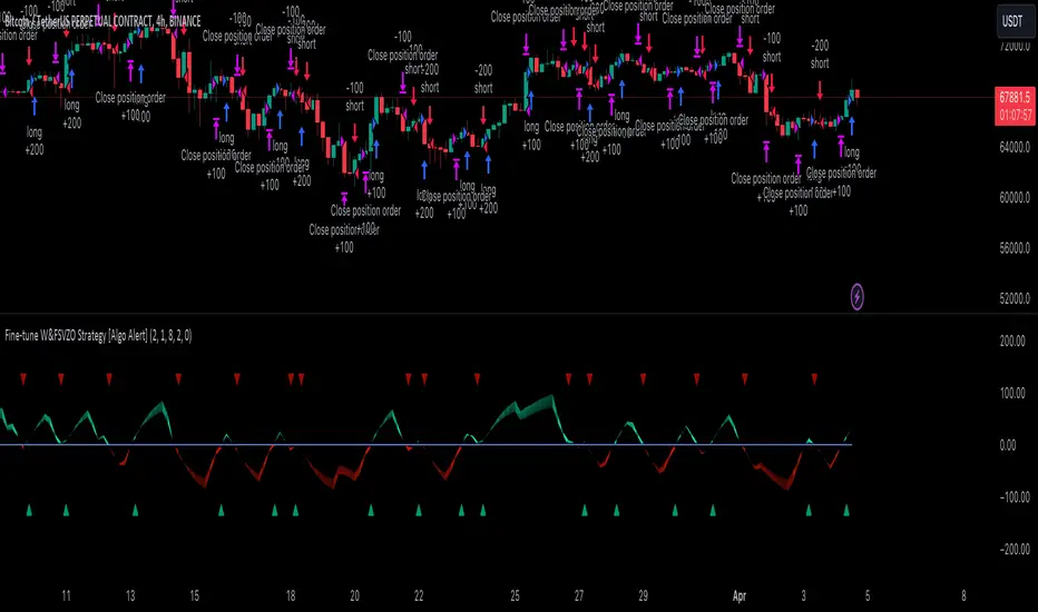
Fine-tune Inputs: Fourier Smoothed Volume zone oscillator WFSVZ0Use this Strategy to Fine-tune inputs for the (W&)FSVZ0 Indicator.
Strategy allows you to fine-tune the indicator for 1 TimeFrame at a time; cross Timeframe Input fine-tuning is done manually after exporting the chart data.
I suggest using "Close all" input False when fine-tuning Inputs for 1 TimeFrame. When you export data to Excel/Numbers/GSheets I suggest using "Close all" input as True, except for the lowest TimeFrame.
MEANINGFUL DESCRIPTION:
The Volume Zone oscillator breaks up volume activity into positive and negative categories. It is positive when the current closing price is greater than the prior closing price and negative when it's lower than the prior closing price. The resulting curve plots through relative percentage levels that yield a series of buy and sell signals, depending on level and indicator direction.
The Wavelet & Fourier Smoothed Volume Zone Oscillator (W&)FSVZO is a refined version of the Volume Zone Oscillator, enhanced by the implementation of the Discrete Fourier Transform . Its primary function is to streamline price data and diminish market noise, thus offering a clearer and more precise reflection of price trends.
By combining the Wavalet and Fourier aproximation with Ehler's white noise histogram, users gain a comprehensive perspective on volume-related market conditions.
HOW TO USE THE INDICATOR:
The default period is 2 but can be adjusted after backtesting. (I suggest 5 VZO length and NoiceR max length 8 as-well)
The VZO points to a positive trend when it is rising above the 0% level, and a negative trend when it is falling below the 0% level. 0% level can be adjusted in setting by adjusting VzoDifference. Oscillations rising below 0% level or falling above 0% level result in a natural trend.
HOW TO USE THE STRATEGY:
Here you fine-tune the inputs until you find a combination that works well on all Timeframes you will use when creating your Automated Trade Algorithmic Strategy. I suggest 4h, 12h, 1D, 2D, 3D, 4D, 5D, 6D, W and M.
When I ndicator/Strategy returns 0 or natural trend , Strategy Closes All it's positions.
ORIGINALITY & USFULLNESS:
Personal combination of Fourier and Wavalet aproximation of a price which results in less noise Volume Zone Oscillator.
The Wavelet Transform is a powerful mathematical tool for signal analysis, particularly effective in analyzing signals with varying frequency or non-stationary characteristics. It dissects a signal into wavelets, small waves with varying frequency and limited duration, providing a multi-resolution analysis. This approach captures both frequency and location information, making it especially useful for detecting changes or anomalies in complex signals.
The Discrete Fourier Transform (DFT) is a mathematical technique that transforms discrete data from the time domain into its corresponding representation in the frequency domain. This process involves breaking down a signal into its individual frequency components, thereby exposing the amplitude and phase characteristics inherent in each frequency element.
This indicator utilizes the concept of Ehler's Universal Oscillator and displays a histogram, offering critical insights into the prevailing levels of market noise. The Ehler's Universal Oscillator is grounded in a statistical model that captures the erratic and unpredictable nature of market movements. Through the application of this principle, the histogram aids traders in pinpointing times when market volatility is either rising or subsiding.
DETAILED DESCRIPTION:
My detailed description of the indicator and use cases which I find very valuable.
What is oscillator?
Oscillators are chart indicators that can assist a trader in determining overbought or oversold conditions in ranging (non-trending) markets.
What is volume zone oscillator?
Price Zone Oscillator measures if the most recent closing price is above or below the preceding closing price.
Volume Zone Oscillator is Volume multiplied by the 1 or -1 depending on the difference of the preceding 2 close prices and smoothed with Exponential moving Average.
What does this mean?
If the VZO is above 0 and VZO is rising. We have a bullish trend. Most likely.
If the VZO is below 0 and VZO is falling. We have a bearish trend. Most likely.
Rising means that VZO on close is higher than the previous day.
Falling means that VZO on close is lower than the previous day.
What if VZO is falling above 0 line?
It means we have a high probability of a bearish trend.
Thus the indicator returns 0 and Strategy closes all it's positions when falling above 0 (or rising bellow 0) and we combine higher and lower timeframes to gauge the trend.
In the next Image you can see that trend is negative on 4h, negative on 12h and positive on 1D. That means trend is negative.
I am sorry, the chart is a bit messy. The idea is to use the indicator over more than 1 Timeframe.
What is approximation and smoothing?
They are mathematical concepts for making a discrete set of numbers a
continuous curved line.
Fourier and Wavelet approximation of a close price are taken from aprox library.
Key Features:
You can tailor the Indicator/Strategy to your preferences with adjustable parameters such as VZO length, noise reduction settings, and smoothing length.
Volume Zone Oscillator (VZO) shows market sentiment with the VZO, enhanced with Exponential Moving Average (EMA) smoothing for clearer trend identification.
Noise Reduction leverages Euler's White noise capabilities for effective noise reduction in the VZO, providing a cleaner and more accurate representation of market dynamics.
Choose between the traditional Fast Fourier Transform (FFT) , the innovative Double Discrete Fourier Transform (DTF32) and Wavelet soothed Fourier soothed price series to suit your analytical needs.
Image of Wavelet transform with FAST settings, Double Fourier transform with FAST settings. Improved noice reduction with SLOW settings, and standard FSVZO with SLOW settings:
Fast setting are setting by default:
VZO length = 2
NoiceR max Length = 2
Slow settings are:
VZO length = 5 or 7
NoiceR max Length = 8
As you can see fast setting are more volatile. I suggest averaging fast setting on 4h 12h 1d 2d 3d 4d W and M Timeframe to get a clear view on market trend.
What if I want long only when VZO is rising and above 15 not 0?
You have set Setting VzoDifference to 15. That reduces the number of trend changes.
Example of W&FSVZO with VzoDifference 15 than 0:
VZO crossed 0 line but not 15 line and that's why Indicator returns 0 in one case an 1 in another.
What is Smooth length setting?
A way of calculating Bullish or Bearish (W&)FSVZO .
If smooth length is 2 the trend is rising if:
rising = VZO > ta.ema(VZO, 2)
Meaning that we check if VZO is higher that exponential average of the last 2 elements.
If smooth length is 1 the trend is rising if:
rising = VZO_ > VZO_
Use this Strategy to fine-tune inputs for the (W&)FSVZO Indicator.
(Strategy allows you to fine-tune the indicator for 1 TimeFrame at a time; cross Timeframe Input fine-tuning is done manually after exporting the chart data)
I suggest using " Close all " input False when fine-tuning Inputs for 1 TimeFrame . When you export data to Excel/Numbers/GSheets I suggest using " Close all " input as True , except for the lowest TimeFrame . I suggest using 100% equity as your default quantity for fine-tune purposes. I have to mention that 100% equity may lead to unrealistic backtesting results. Be avare. When backtesting for trading purposes use Contracts or USDT.
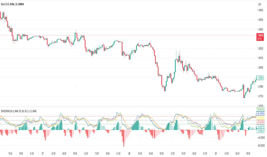
[KVA] Kamvia Directional MovementKamvia Directional Movement (KDM) Indicator is an analytical tool designed to identify potential buying and selling opportunities in the market. It highlights the phases of price depletion which typically align with price highs and lows, offering a nuanced understanding of market dynamics.
Efficient at pinpointing trend breakdowns and excelling in the identification of intra-day entry and exit points, the Kamvia Directional Movement Indicator is a valuable asset for traders aiming to optimize their market strategies.
The KDM not only takes into account the traditional high and low price points within its analysis but also introduces an innovative approach by incorporating the concepts of body high and body low. This nuanced analysis offers a deeper insight into market momentum and potential shifts in market dynamics.
High and Low Analysis : The indicator examines the price highs and lows to gauge the overall market volatility and potential turning points. By analyzing these extremities, traders can get a sense of market strength and possible shifts in trend direction. The high points indicate periods of maximum buying interest, potentially signaling overbought conditions, while the low points reflect selling interest, hinting at oversold conditions.
Body High and Body Low Analysis : Unique to the KDM Indicator is the emphasis on the body of the candlestick, which is the range between the open and close prices. This analysis offers a more refined view of market sentiment by focusing on the actual trading range experienced within the period. The body high (the upper end of the candlestick body) and body low (the lower end of the candlestick body) provide insights into the buying and selling pressure during the trading session, beyond mere price extremities.
The indicator is calibrated on a scale from 0 to 100, making interpretation intuitive and straightforward. A reading above 70 is considered to be in the overbought region, suggesting that the market might be experiencing a heightened level of buying activity that could lead to a potential pullback or reversal. Conversely, a reading below 30 falls into the oversold region, indicating a possible exhaustion in selling pressure and a potential for market reversal or bounce back.
This scale and the detailed analysis of both price and body dynamics equip traders with a comprehensive tool for assessing market conditions. The distinction between high/low and body high/body low analysis enriches the indicator's capability to provide more targeted insights into market behavior, enabling traders to make more nuanced decisions based on a broader spectrum of information. By identifying the duration and extent to which these conditions persist, traders can better interpret the market's momentum and align their strategies with the prevailing trend or prepare for an impending reversal.
KDM Strategy
The strategy focuses on spotting price reversals within a confirmed trend. While the indicator features regions indicating overbought and oversold conditions, these signals alone are not sufficient predictors of a market reversal.
The terms "overbought" and "oversold" describe scenarios where prices reach levels that are unusually high or low within a specified look-back period. Entering these zones often indicates a continuation of the trend rather than a reversal.
A "strongly overbought" condition signals buying pressure, whereas a "strongly oversold" condition indicates selling pressure. The key to leveraging these conditions lies in analyzing the duration for which the market remains in either state. This duration can provide critical insights into whether the market is trending or ranging.
Extended periods in extreme overbought territories confirm an uptrend, while prolonged presence in slight overbought zones (above 50 but below 70, for example) suggests a more moderate uptrend. Conventionally, levels above 70 signal extreme overbought conditions, and those below 30 indicate extreme oversold conditions.
Traders are advised to exercise caution when the oscillator stays within these extreme areas. Ideally, the strategy involves capitalizing on temporary price drops within an overall uptrend or on temporary price spikes within an overall downtrend.
Identifying trading opportunities with the KDM Indicator involves looking for the indicator to exit these extreme overbought or oversold regions, signaling potential reversals or continuations in the market's direction. This approach helps traders make informed decisions by considering the broader market trend alongside short-term price movements.
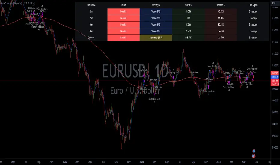
Kyrie Crossover ( @zaytradellc )Unlocking Market Dynamics: Kyrie Crossover Script by @zaytradellc
personalized trading success with the "Kyrie Crossover" script, meticulously crafted by @zaytrade. This innovative Pine Script, tailored to the birthdays of Kyrie and the script creator, combines the power of technical analysis with a touch of personalization to revolutionize your trading experience.
**Exponential Moving Average (EMA) Crossover Strategy:**
At the heart of the "Kyrie Crossover" script lies a sophisticated EMA crossover strategy. By utilizing a 10-period EMA and a 323-period EMA (symbolizing long term price action ), the strategy effectively captures market trends with precision and insight.
- **Short-Term EMA (10-period):** This EMA reacts swiftly to recent price changes, offering heightened sensitivity to short-term fluctuations. It excels in identifying immediate shifts in market sentiment, making it invaluable for pinpointing short-lived trends and potential reversal points.
- **Long-Term EMA (323-period):** In contrast, the long-term EMA provides a broader perspective by smoothing out short-term noise and focusing on longer-term trend direction. Its extended length filters out market noise effectively, providing a clear representation of the underlying trend's momentum and sustainability.
**Directional Movement Index (DMI) Metrics:**
The "Kyrie Crossover" script goes beyond traditional indicators by incorporating DMI metrics across multiple timeframes. By assessing trend strength and direction, traders gain valuable insights into market dynamics, allowing for informed decision-making.
**Simple Instructions to Profit:**
1. **Identify EMA Crossovers:** Look for instances where the short-term EMA (10-period) crosses above the long-term EMA (323-period) for a bullish signal, indicating a potential buying opportunity. Conversely, a crossover where the short-term EMA crosses below the long-term EMA signals a bearish trend and a potential selling opportunity.
2. **Confirm with DMI Metrics:** Validate EMA crossovers by checking DMI metrics across different timeframes (5 minutes, 15 minutes, 30 minutes, and 1 hour). Pay attention to color-coded indicators, with green indicating a bullish trend, red indicating a bearish trend, and white indicating no clear trend.
3. **Manage Risk:** Implement proper risk management techniques, such as setting stop-loss orders and position sizing based on your risk tolerance and trading objectives.
4. **Stay Informed:** Regularly monitor market conditions and adjust your trading strategy accordingly based on new signals and emerging trends.
Inside Candle StrategyIntroduction
The Inside Candle Breakout Strategy leverages the concept of inside candles as a primary signal for potential breakouts. Unlike common trend-following or scalping strategies, this method focuses on the volatility squeeze indicated by inside candles and aims to capture the momentum that follows these periods of consolidation. The strategy's originality lies in its specific integration of timeframes for signal detection and its application across diverse market conditions without relying on conventional trend indicators.
Strategy Description and Mechanics
Inside Candle Identification: At the heart of this strategy is the detection of inside candles, defined as candles fully contained within the range of the preceding candle. This pattern signifies a temporary balance between buyers and sellers, often preceding significant price movements. The strategy scans for these candles within a user-specified timeframe in the input section of the settings of the strategy, allowing for tailored signal generation based on individual trading preferences.
Entry Points and Market Entries: Upon identifying an inside candle and only once this candle closes, the strategy prepares to enter a trade in the direction of the breakout. Trades are executed in the timeframe selected on the chart, ensuring that entry points are aligned with real-time market movements. This process highlights the strategy's adaptability, making it suitable for various trading styles, from day trading to swing trading.
Overlay Indicator for Enhanced Market Analysis: Accompanying the breakout signals is an overlay indicator comprising two moving averages and a volatility cloud. This feature serves as a secondary tool for market analysis, offering insights into the prevailing market trend and volatility levels. While it doesn't influence the entry or exit signals directly, it provides traders with additional context for refining their decisions, enhancing the strategy's utility. This assistance tool is composed by one moving average and a second line which is calculated adding or subtracting the historical volatility of the asset on the moving average, depending on his momentum.
Strategy Results and Commitment to Realism
Backtesting Protocol: In our commitment to transparency and realism, backtesting results are derived from a dataset that ensures a sufficient number of trades (over 100) to validate the strategy's effectiveness. This approach underscores our dedication to providing traders with reliable and actionable insights.
Risk Management and Trade Sizing: Recognizing the importance of sustainable trading practices, the strategy incorporates strict risk management guidelines. Trades are sized to ensure that only a small percentage of equity is risked on a single trade, adhering to widely accepted risk tolerance levels. The initial account size for this script is set to 10000$.
Strategy Defaults and Justification: The default properties of the strategy, including the risk-reward ratio, average length for moving averages, and other parameters, are carefully chosen based on extensive testing and analysis. These settings represent a balanced approach, aiming to optimize the strategy's performance across a variety of market conditions.
Strategy Components:
- Inside Candles: An inside candle occurs when a candle's high and low are completely contained within the high and low of the previous candle. This pattern indicates a period of consolidation or indecision in the market, often preceding a significant price movement. The strategy detects inside candles based on the user-selected timeframe, allowing traders to capture potential breakouts.
Indicator Overlays:
- Moving Average: A simple moving average (SMA) is calculated over a user-defined length (`Average Length`), providing a dynamic baseline to gauge the market's direction. The strategy offers an option (`Show Moving Average`) to display or hide this moving average on the chart, giving traders control over the visual complexity.
- Volatility Measurement: Alongside the moving average, the strategy assesses market volatility using the standard deviation of the closing prices over the same period defined by the `Average Length`. The moving average is adjusted upwards or downwards by this volatility measure, creating a dynamic channel that reflects the current market conditions.
- Color Gradients for Volatility: The strategy uses a color gradient to fill the area between the moving average and its volatility-adjusted counterpart. This gradient visually represents the volatility level, transitioning from gray (low volatility) to a lighter shade (higher volatility), aiding in the assessment of market sentiment and volatility.
Trading Entries:
- Long Entry: A long position is triggered when the closing price exceeds the high of an inside candle, indicating potential bullish momentum. The strategy places a stop-loss at the low of the inside candle and sets a take-profit level based on the predefined risk-reward ratio (`RR Ratio`).
- Short Entry: Conversely, a short position is initiated when the closing price falls below the low of an inside candle, suggesting bearish pressure. A stop-loss is set at the high of the inside candle, with the take-profit level adjusted according to the risk-reward ratio.
Customization Settings:
- Timeframe: Traders can select the desired timeframe for inside candle detection, tailoring the strategy to fit various trading styles and time horizons.
- RR Ratio: The risk-reward ratio is adjustable, allowing traders to manage the potential risk and return of each trade according to their risk tolerance.
- Average Length: This setting determines the period over which the moving average and volatility are calculated, affecting the sensitivity of the strategy to price movements.
- Visual Settings: Users can customize the appearance of the strategy on their charts, including the colors of the moving average and volatility lines, as well as the line width, enhancing chart readability and personal preference adherence.
Disclaimer
Trading involves significant risk, and it is crucial for traders to conduct their own due diligence before engaging with any strategy. The Inside Candle Breakout Strategy is presented for informational purposes only and does not constitute financial advice.

Trend Deviation strategy - BTC [IkkeOmar]Intro:
This is an example if anyone needs a push to get started with making strategies in pine script. This is an example on BTC, obviously it isn't a good strategy, and I wouldn't share my own good strategies because of alpha decay.
This strategy integrates several technical indicators to determine market trends and potential trade setups. These indicators include:
Directional Movement Index (DMI)
Bollinger Bands (BB)
Schaff Trend Cycle (STC)
Moving Average Convergence Divergence (MACD)
Momentum Indicator
Aroon Indicator
Supertrend Indicator
Relative Strength Index (RSI)
Exponential Moving Average (EMA)
Volume Weighted Average Price (VWAP)
It's crucial for you guys to understand the strengths and weaknesses of each indicator and identify synergies between them to improve the strategy's effectiveness.
Indicator Settings:
DMI (Directional Movement Index):
Length: This parameter determines the number of bars used in calculating the DMI. A higher length may provide smoother results but might lag behind the actual price action.
Bollinger Bands:
Length: This parameter specifies the number of bars used to calculate the moving average for the Bollinger Bands. A longer length results in a smoother average but might lag behind the price action.
Multiplier: The multiplier determines the width of the Bollinger Bands. It scales the standard deviation of the price data. A higher multiplier leads to wider bands, indicating increased volatility, while a lower multiplier results in narrower bands, suggesting decreased volatility.
Schaff Trend Cycle (STC):
Length: This parameter defines the length of the STC calculation. A longer length may result in smoother but slower-moving signals.
Fast Length: Specifies the length of the fast moving average component in the STC calculation.
Slow Length: Specifies the length of the slow moving average component in the STC calculation.
MACD (Moving Average Convergence Divergence):
Fast Length: Determines the number of bars used to calculate the fast EMA (Exponential Moving Average) in the MACD.
Slow Length: Specifies the number of bars used to calculate the slow EMA in the MACD.
Signal Length: Defines the number of bars used to calculate the signal line, which is typically an EMA of the MACD line.
Momentum Indicator:
Length: This parameter sets the number of bars over which momentum is calculated. A longer length may provide smoother momentum readings but might lag behind significant price changes.
Aroon Indicator:
Length: Specifies the number of bars over which the Aroon indicator calculates its values. A longer length may result in smoother Aroon readings but might lag behind significant market movements.
Supertrend Indicator:
Trendline Length: Determines the length of the period used in the Supertrend calculation. A longer length results in a smoother trendline but might lag behind recent price changes.
Trendline Factor: Specifies the multiplier used in calculating the trendline. It affects the sensitivity of the indicator to price changes.
RSI (Relative Strength Index):
Length: This parameter sets the number of bars over which RSI calculates its values. A longer length may result in smoother RSI readings but might lag behind significant price changes.
EMA (Exponential Moving Average):
Fast EMA: Specifies the number of bars used to calculate the fast EMA. A shorter period results in a more responsive EMA to recent price changes.
Slow EMA: Determines the number of bars used to calculate the slow EMA. A longer period results in a smoother EMA but might lag behind recent price changes.
VWAP (Volume Weighted Average Price):
Default settings are typically used for VWAP calculations, which consider the volume traded at each price level over a specific period. This indicator provides insights into the average price weighted by trading volume.
backtest range and rules:
You can specify the start date for backtesting purposes.
You can can select the desired trade direction: Long, Short, or Both.
Entry and Exit Conditions:
LONG:
DMI Cross Up: The Directional Movement Index (DMI) indicates a bullish trend when the positive directional movement (+DI) crosses above the negative directional movement (-DI).
Bollinger Bands (BB): The price is below the upper Bollinger Band, indicating a potential reversal from the upper band.
Momentum Indicator: Momentum is positive, suggesting increasing buying pressure.
MACD (Moving Average Convergence Divergence): The MACD line is above the signal line, indicating bullish momentum.
Supertrend Indicator: The Supertrend indicator signals an uptrend.
Schaff Trend Cycle (STC): The STC indicates a bullish trend.
Aroon Indicator: The Aroon indicator signals a bullish trend or crossover.
When all these conditions are met simultaneously, the strategy considers it a favorable opportunity to enter a long trade.
SHORT:
DMI Cross Down: The Directional Movement Index (DMI) indicates a bearish trend when the negative directional movement (-DI) crosses above the positive directional movement (+DI).
Bollinger Bands (BB): The price is above the lower Bollinger Band, suggesting a potential reversal from the lower band.
Momentum Indicator: Momentum is negative, indicating increasing selling pressure.
MACD (Moving Average Convergence Divergence): The MACD line is below the signal line, signaling bearish momentum.
Supertrend Indicator: The Supertrend indicator signals a downtrend.
Schaff Trend Cycle (STC): The STC indicates a bearish trend.
Aroon Indicator: The Aroon indicator signals a bearish trend or crossover.
When all these conditions align, the strategy considers it an opportune moment to enter a short trade.
Disclaimer:
THIS ISN'T AN OPTIMAL STRATEGY AT ALL! It was just an old project from when I started learning pine script!
The backtest doesn't promise the same results in the future, always do both in-sample and out-of-sample testing when backtesting a strategy. And make sure you forward test it as well before implementing it!
Furthermore this strategy uses both trend and mean-reversion systems, that is usually a no-go if you want to build robust trend systems .
Don't hesitate to comment if you have any questions or if you have some good notes for a beginner.

Aroon and ASH strategy - ETHERIUM [IkkeOmar]Intro:
This post introduces a Pine Script strategy, as an example if anyone needs a push to get started. This example is a strategy on ETH, obviously it isn't a good strategy, and I wouldn't share my own good strategies because of alpha decay. This strategy combines two technical indicators: Aroon and Absolute Strength Histogram (ASH).
Overview:
The strategy employs the Aroon indicator alongside the Absolute Strength Histogram (ASH) to determine market trends and potential trade setups. Aroon helps identify the strength and direction of a trend, while ASH provides insights into the strength of momentum. By combining these indicators, the strategy aims to capture profitable trading opportunities in Ethereum markets. Normally when developing strats using indicators, you want to find some good indicators, but you NEED to understand their strengths and weaknesses, other indicators can be incorporated to minimize the downs of another indicator. Try to look for synergy in your indicators!
Indicator settings:
Aroon Indicator:
- Two sets of parameters are used for the Aroon indicator:
- For Long Positions: Aroon periods are set to 56 (upper) and 20 (lower).
- For Short Positions: Aroon periods are set to 17 (upper) and 55 (lower).
Absolute Strength Histogram (ASH):
ASH is calculated with a length of 9 bars using the closing price as the data source.
Trading Conditions:
The strategy incorporates specific conditions to initiate and exit trades:
Start Date:
Traders can specify the start date for backtesting purposes.
Trade Direction:
Traders can select the desired trade direction: Long, Short, or Both.
Entry and Exit Conditions:
1. Long Position Entry: A long position is initiated when the Aroon indicator crosses over (crossover) the lower Aroon threshold, indicating a potential uptrend.
2. Long Position Exit: A long position is closed when the Aroon indicator crosses under (crossunder) the lower Aroon threshold.
3. Short Position Entry: A short position is initiated when the Aroon indicator crosses under (crossunder) the upper Aroon threshold, signaling a potential downtrend.
4. Short Position Exit: A short position is closed when the Aroon indicator crosses over (crossover) the upper Aroon threshold.
Disclaimer:
THIS ISN'T AN OPTIMAL STRATEGY AT ALL! It was just an old project from when I started learning pine script!
The backtest doesn't promise the same results in the future, always do both in-sample and out-of-sample testing when backtesting a strategy. And make sure you forward test it as well before implementing it!

PresentTrend RMI Synergy - Strategy [presentTrading] █ Introduction and How it is Different
The "PresentTrend RMI Synergy Strategy" is the combined power of the Relative Momentum Index (RMI) and a custom presentTrend indicator. This strategy introduces a multifaceted approach, integrating momentum analysis with trend direction to offer traders a more nuanced and responsive trading mechanism.
BTCUSD 6h L/S Performance
Local
█ Strategy, How It Works: Detailed Explanation
The "PresentTrend RMI Synergy Strategy" intricately combines the Relative Momentum Index (RMI) and a custom SuperTrend indicator to create a powerful tool for traders.
🔶 Relative Momentum Index (RMI)
The RMI is a variation of the Relative Strength Index (RSI), but instead of using price closes against itself, it measures the momentum of up and down movements in price relative to previous prices over a given period. The RMI for a period length `N` is calculated as follows:
RMI = 100 - 100/ (1 + U/D)
where:
- `U` is the average upward price change over `N` periods,
- `D` is the average downward price change over `N` periods.
The RMI oscillates between 0 and 100, with higher values indicating stronger upward momentum and lower values suggesting stronger downward momentum.
RMI = 21
RMI = 42
For more information - RMI Trend Sync - Strategy :
🔶 presentTrend Indicator
The presentTrend indicator combines the Average True Range (ATR) with a moving average to determine trend direction and dynamic support or resistance levels. The presentTrend for a period length `M` and a multiplier `F` is defined as:
- Upper Band: MA + (ATR x F)
- Lower Band: MA - (ATR x F)
where:
- `MA` is the moving average of the close price over `M` periods,
- `ATR` is the Average True Range over the same period,
- `F` is the multiplier to adjust the sensitivity.
The trend direction switches when the price crosses the presentTrend bands, signaling potential entry or exit points.
presentTrend length = 3
presentTrend length = 10
For more information - PresentTrend - Strategy :
🔶 Strategy Logic
Entry Conditions:
- Long Entry: Triggered when the RMI exceeds a threshold, say 60, indicating a strong bullish momentum, and when the price is above the presentTrend, confirming an uptrend.
- Short Entry: Occurs when the RMI drops below a threshold, say 40, showing strong bearish momentum, and the price is below the present trend, indicating a downtrend.
Exit Conditions with Dynamic Trailing Stop:
- Long Exit: Initiated when the price crosses below the lower presentTrend band or when the RMI falls back towards a neutral level, suggesting a weakening of the bullish momentum.
- Short Exit: Executed when the price crosses above the upper presentTrend band or when the RMI rises towards a neutral level, indicating a reduction in bearish momentum.
Equations for Dynamic Trailing Stop:
- For Long Positions: The exit price is set at the lower SuperTrend band once the entry condition is met.
- For Short Positions: The exit price is determined by the upper SuperTrend band post-entry.
These dynamic trailing stops adjust as the market moves, providing a method to lock in profits while allowing room for the position to grow.
This strategy's strength lies in its dual analysis approach, leveraging RMI for momentum insights and presentTrend for trend direction and dynamic stops. This combination offers traders a robust framework to navigate various market conditions, aiming to capture trends early and exit positions strategically to maximize gains and minimize losses.
█ Trade Direction
The strategy provides flexibility in trade direction selection, offering "Long," "Short," or "Both" options to cater to different market conditions and trader preferences. This adaptability ensures that traders can align the strategy with their market outlook, risk tolerance, and trading goals.
█ Usage
To utilize the "PresentTrend RMI Synergy Strategy," traders should input their preferred settings in the Pine Script™ and apply the strategy to their charts. Monitoring RMI for momentum shifts and adjusting positions based on SuperTrend signals can optimize entry and exit points, enhancing potential returns while managing risk.
█ Default Settings
1. RMI Length: 21
The 21-period RMI length strikes a balance between capturing momentum and filtering out market noise, offering a medium-term outlook on market trends.
2. Super Trend Length: 7
A SuperTrend length of 7 periods is chosen for its responsiveness to price movements, providing a dynamic framework for trend identification without excessive sensitivity.
3. Super Trend Multiplier: 4.0
The multiplier of 4.0 for the SuperTrend indicator widens the trend bands, focusing on significant market moves and reducing the impact of minor fluctuations.
---
The "PresentTrend RMI Synergy Strategy" represents a significant step forward in trading strategy development, blending momentum and trend analysis in a unique way. By providing a detailed framework for understanding market dynamics, this strategy empowers traders to make more informed decisions.

NY Open Breakout Strategy - High Liquidity & Favorable RRR Pine Description:
The NY Open Breakout Strategy is an advanced Pine Script indicator tailored for the TradingView platform. This strategy is specifically designed to exploit the high liquidity found during the New York session opening in the Forex market. Its primary goal is to provide traders with an opportunity to engage in positions with lower risk and higher potential profits, thereby ensuring an advantageous risk-to-reward ratio (RRR).
Core Objectives:
Leveraging High Liquidity: Capitalizes on the significant market movements at the New York session opening, known for its high liquidity, to identify strong breakout signals.
Achieving Favorable RRR: By setting strategic stop-loss and take-profit levels, the strategy aims for a higher RRR. This approach can lead to overall profitability, even if the win rate is lower than the loss rate.
Functionality:
Dynamic Breakout Identification: Uses the first 15-minute candle’s high and low after NY open as benchmarks for detecting potential breakouts.
Customizable Stop-Loss & Take-Profit: Provides options to configure stop-loss at the last swing or the previous candle’s close. The take-profit levels are determined based on a favorable risk-reward ratio.
Visual Session Indicators: Includes distinct background coloring and vertical lines to mark the New York session for easy visibility.
Methodology:
This strategy hinges on the premise that the opening of the New York session often triggers key price movements due to an influx of trading activity. By focusing on these moments, our indicator aims to capture strong trends and breakout patterns. The carefully calibrated stop-loss and take-profit settings ensure that each trade aims for a higher potential reward compared to the risk undertaken.
Unique Features:
Enhanced Risk Management: With adaptable risk-reward settings, traders can tailor their trading strategies to align with individual risk appetites.
Personalized User Experience: Offers a range of customizable settings for visual elements, allowing traders to adjust the look and feel of the indicator to their preferences.
Usage Guidelines:
Customize the indicator settings, including the stop-loss reference and risk-reward ratio, to match your trading style.
Watch for 'Buy Enter' and 'Sell Enter' signals during the New York session opening.
Utilize the displayed stop-loss and take-profit levels to effectively manage each trade.
This NY Open Breakout Strategy is ideal for traders who prioritize efficient risk management while aiming to capitalize on the high liquidity periods of the Forex market. The strategy is designed to be robust, providing a pathway to profitability even in scenarios where the number of losing trades surpasses winning ones, thanks to its emphasis on a high risk-to-reward ratio.

QQE MOD + SSL Hybrid + Waddah Attar Explosion IndicatorINDICATOR PURPOSE
This indicator is designed to complement my original QQE MOD + SSL Hybrid + Waddah Attar Explosion strategy.
Multiple users have requested that I convert the strategy to an indicator because alertconditions do not work on strategies and people want to specific set alerts for BUY, SELL, CLOSE BUY and CLOSE SELL. This can only be achieved using alertcondition().
This indicator functions in the exact same way as the strategy, but it doesn't have any backtesting functionality. I recomment that you use the original QQE MOD + SSL Hybrid + Waddah Attar Explosion strategy for parameter tuning and backtesting, then if you need more control on alerts you can use this indicator for that purpose.
Only other difference is that I have added grey exit labels on the chart since it's not obvious where the exits would happen like it was in the strategy version.
CREDITS
QQE MOD byMihkel00
SSL Hybrid by Mihkel00
Waddah Attar Explosion by shayankm

PKJ StrategyWelcome to the Daily Price Action Mastery Strategy, a powerful approach to navigating the financial markets using the purest form of market analysis – price action. This trading view strategy is meticulously crafted for those seeking a method that harnesses the daily price movements to make informed and strategic trading decisions.
Key Features:
Daily Candlestick Analysis: Dive into the daily candlestick patterns to identify key support and resistance levels, trend reversals, and potential breakout points. The strategy leverages the valuable information encapsulated in each day's price action to discern market sentiment.
Trend Identification: Utilize trend analysis tools and indicators to pinpoint the prevailing market direction. By understanding the dynamics of daily trends, traders can align their positions with the broader market movement for higher probability trades.
Dynamic Support and Resistance: Implement dynamic support and resistance levels derived from daily price action. These levels act as crucial markers for entry and exit points, helping traders set effective stop-loss and take-profit orders.
Chart Patterns Recognition: Uncover chart patterns such as head and shoulders, flags, and triangles on the daily timeframe. The strategy incorporates pattern recognition techniques to identify potential trend continuation or reversal scenarios, offering traders a comprehensive view of market dynamics.
Volatility Analysis: Gauge market volatility by studying daily price ranges and fluctuations. Volatility indicators are integrated to help traders adjust their risk management strategies in response to varying market conditions.
Confirmation through Indicators: Supplement price action analysis with carefully selected indicators for additional confirmation signals. These indicators are chosen to align with the philosophy of the Daily Price Action Mastery Strategy, enhancing the precision of trade entries and exits.
Risk Management Guidelines: Discover effective risk management practices tailored to the daily timeframe. Learn how to optimize position sizes, set appropriate stop-loss levels, and manage capital to ensure long-term success and sustainability in your trading journey.
Whether you are a seasoned trader or a newcomer to the markets, the Daily Price Action Mastery Strategy provides a comprehensive framework to navigate the complexities of daily price movements. Elevate your trading experience by incorporating this strategy into your analysis, and empower yourself to make well-informed decisions in the dynamic world of finance.

FlexiMA x FlexiST - Strategy [presentTrading]█ Introduction and How it is Different
The FlexiMA x FlexiST Strategy blends two analytical methods - FlexiMA and FlexiST, which are opened in my early post.
- FlexiMA calculates deviations between an indicator source and a dynamic moving average, controlled by a starting factor and increment factor.
- FlexiST, on the other hand, leverages the SuperTrend model, adjusting the Average True Range (ATR) length for a comprehensive trend-following oscillator.
This synergy offers traders a more nuanced and multifaceted tool for market analysis.
BTC 6H L/S Performance
Local
█ Strategy, How It Works: Detailed Explanation
The strategy combines two components: FlexiMA and FlexiST, each utilizing unique methodologies to analyze market trends.
🔶FlexiMA Component:
- Calculates deviations between an indicator source and moving averages of variable lengths.
- Moving average lengths are dynamically adjusted using a starting factor and increment factor.
- Deviations are normalized and analyzed to produce median and standard deviation values, forming the FlexiMA oscillator.
Length indicator (50)
🔶FlexiST Component:
- Uses SuperTrend indicators with varying ATR (Average True Range) lengths.
- Trends are identified based on the position of the indicator source relative to the SuperTrend bands.
- Deviations between the indicator source and SuperTrend values are calculated and normalized.
Starting Factor (5)
🔶Combined Strategy Logic:
- Entry Signals:
- Long Entry: Triggered when median values of both FlexiMA and FlexiST are positive.
- Short Entry: Triggered when median values of both FlexiMA and FlexiST are negative.
- Exit Signals:
- Long Exit: Triggered when median values of FlexiMA or FlexiST turn negative.
- Short Exit: Triggered when median values of FlexiMA or FlexiST turn positive.
This strategic blend of FlexiMA and FlexiST allows for a nuanced analysis of market trends, providing traders with signals based on a comprehensive view of market momentum and trend strength.
█ Trade Direction
The strategy is designed to cater to various trading preferences, offering "Long", "Short", and "Both" options. This flexibility allows traders to align the strategy with their specific market outlook, be it bullish, bearish, or a combination of both.
█ Usage
Traders can effectively utilize the FlexiMA x FlexiST Strategy by first selecting their desired trade direction. The strategy then generates entry signals when the conditions for either the FlexiMA or FlexiST are met, indicating potential entry points in the market. Conversely, exit signals are generated when the conditions for these indicators diverge, thus signaling a potential shift in market trends and suggesting a strategic exit point.
█ Default Settings
1. Indicator Source (HLC3): Provides a balanced and stable price source, reducing the impact of extreme market fluctuations.
2. Indicator Lengths (20 for FlexiMA, 10 for FlexiST): Longer FlexiMA length smooths out short-term fluctuations, while shorter FlexiST length allows for quicker response to market changes.
3. Starting Factors (1.0 for FlexiMA, 0.618 for FlexiST): Balanced start for FlexiMA and a harmonized approach for FlexiST, resonating with natural market cycles.
4. Increment Factors (1.0 for FlexiMA, 0.382 for FlexiST): FlexiMA captures a wide range of market behaviors, while FlexiST provides a gradual transition to capture finer trend shifts.
5. Normalization Methods ('None'): Uses raw deviations, suitable for markets where absolute price movements are more significant.
6. Trade Direction ('Both'): Allows strategy to consider both long and short opportunities, ideal for versatile market engagement.
*More details:
1. FlexiMA
2. FlexiST

Envelope and Moving Average**Description:**
- This script creates an indicator that combines an envelope and a simple moving average (MA).
- The envelope is constructed using a specified length, percentage deviation, and source price (close by default).
- The moving average is calculated based on a specified length and source price.
**Inputs:**
1. Envelope:
- Length: Number of periods used for the envelope calculation (default is 20).
- Percentage Deviation: Percentage above and below the envelope basis (default is 10%).
- Source: The price used for the envelope calculation (default is close).
- Exponential MA: Option to use exponential moving average for the envelope basis (default is false).
2. Moving Average:
- Length: Number of periods used for the moving average calculation (default is 20).
- Source: The price used for the moving average calculation (default is close).
**Plotting:**
- The script plots the envelope basis, upper envelope line, and lower envelope line.
- The area between the upper and lower envelope lines is filled with a semi-transparent color for better visualization.
- The moving average is plotted on the chart with a specified color and line width.
**How to Use in a Strategy:**
1. **Envelope Crossovers:**
- Go Long (Buy): When the close price crosses above the upper envelope line.
- Go Short (Sell): When the close price crosses below the lower envelope line.
2. **Moving Average Crossovers:**
- Go Long (Buy): When the close price crosses above the moving average.
- Go Short (Sell): When the close price crosses below the moving average.
3. **Confirmation:**
- Consider additional confirmation signals or filters to improve the robustness of your strategy.
- For example, you might require a certain amount of price momentum or use other technical indicators in conjunction with envelope and moving average signals.
4. **Optimization:**
- Experiment with different parameter values (e.g., envelope length, percentage deviation, moving average length) to optimize the strategy for specific market conditions.
5. **Risk Management:**
- Implement proper risk management techniques, such as setting stop-loss orders and position sizing, to control risk.
Remember to thoroughly backtest any strategy before deploying it in a live trading environment. Additionally, consider the current market conditions and adapt your strategy accordingly.