Nested SMA WaveThe "Nested SMA Wave" is a custom Pine Script (v5) indicator for TradingView that overlays a series of 8 Simple Moving Averages (SMAs) on the price chart. These SMAs use exponentially increasing lengths based on powers of 2, starting from a user-defined base length (default: 25). This creates lengths like 25, 50, 100, 200, 400, 800, 1600, and 3200.
Each SMA is plotted in a distinct color, forming a "wave" of nested lines that fan out from short-term (faster, more responsive) to long-term (slower, smoother). Semi-transparent colored fills (shaded zones) are added between consecutive SMAs, with customizable toggles and transparency levels, creating layered visual bands that highlight the spaces between different trend timescales.
Use Cases
Multi-Timeframe Trend Visualization: The power-of-2 nesting approximates higher timeframe trends on lower timeframes without switching charts. Shorter SMAs react quickly to price changes, while longer ones show major trends, helping identify overall market structure at a glance.
Support/Resistance Identification: Price interacting with the SMA lines or shaded zones can act as dynamic support/resistance. Crossovers between nested SMAs signal potential momentum shifts.
Trend Strength and Alignment: When SMAs are widely spaced and aligned (e.g., all sloping up), it indicates strong trends. Converging or crossing SMAs suggest consolidation or reversals. The shaded zones add depth, making expansions/contractions in volatility or trend power visually obvious.
Ribbon-Style Trading: Similar to moving average ribbons, traders can look for price pulling back to inner zones for entries in the direction of the broader "wave," or use zone breaks for signals.
Customization for Different Assets/Timeframes: Adjust the base length (e.g., smaller for crypto volatility, larger for stocks) and toggle shades to reduce clutter.
This creates a visually rich, rainbow-like overlay that's particularly useful for trend-following strategies on any chart.
Cerca negli script per "wave"

CPR + Elliott Wave 3 Combo (Ultra Safe)This will help you to identify the stage of a script. In Elliot wave patter, 3rd wave is the longest length. This will identify the 3rd wave

Advanced Elliott Wave PlotterAdvanced Elliott Wave plotter, Parameters can be adjusted.
AI Generated, so no particular credits to anyone.


Kelly Wave Position Matrix 20251024 V1 ZENYOUNGA simple table is designed for use when opening a position. It applies the Kelly formula to calculate a more scientific position size based on win rate and risk–reward ratio. At the same time, it displays 1.65× ATR stop-loss levels for both long and short positions to serve as a reference for comparing with existing stop-loss placements.
Additionally, the table back-calculates the corresponding position size based on a 2% total capital loss limit, using the actual loss ratio. It also shows the current wave trend status as a pre-filtering condition.
Overall, this table integrates the core elements of trading — trend (wave confirmation), win rate, risk–reward ratio, and position sizing — making it an effective checklist before entering a trade. Its purpose is to help achieve a probabilistic edge and ensure positive expected value in trading decisions.

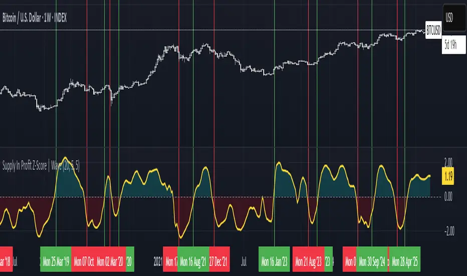
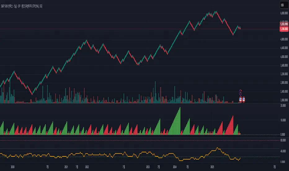
Supply In Profit Z-Score | Wave BackgroundSupply in Profit Z-Score
Modified by Quant_Hustler | Original by QuantChook
What it does
The Supply in Profit Z-Score measures how extreme the balance is between BTC addresses in profit versus those in loss compared to historical norms.
It highlights periods of excessive optimism or pessimism, helping traders identify market sentiment extremes that can signal potential turning points or confirm ongoing trends.
This version is designed for longer-term strategies, using smoothing and statistical normalization to focus on broader market sentiment cycles rather than short-term noise.
How it works
--Data Retrieval: Pulls on-chain data showing the percentage of Bitcoin addresses currently in profit and in loss.
--Spread Calculation: Finds the difference between the two to gauge overall sentiment balance.
--Alpha Decay Adjustment (optional): Normalizes extreme values to stabilize the signal over time.
--Smoothing: Applies a moving average to filter daily volatility and improve long-term clarity.
--Z-Score Conversion: Standardizes the data to show how far current sentiment deviates from historical averages.
--Visualization: Plots the result around a neutral midpoint (zero line) — positive values indicate profit dominance, negative values indicate loss dominance.
How to use it
--Above Zero: More addresses in profit → bullish sentiment and strong trend conditions.
--Below Zero: More addresses in loss → bearish sentiment or potential accumulation zones.
--Extreme Values: Mark overly optimistic or capitulated sentiment, often preceding major reversals.
Why use it in trend following
--This indicator serves as an on-chain sentiment confirmation layer for trend-following systems, especially on higher timeframes (daily or weekly).
--In uptrends, sustained positive readings confirm market strength and investor confidence.
--In downtrends, persistent negative readings confirm weakness and help avoid false reversal signals.
--Divergences between price and sentiment (e.g., rising price but weakening sentiment) often signal momentum loss or potential trend transitions.
Modifications from the original by QuantChook
Added EMA, adaptive Z-score smoothing and capping to reduce volatility and noise.
Introduced a wave-style visualization for intuitive sentiment shifts.
Improved calculation structure and upgraded for Pine Script v6 efficiency.
Tuned signal responsiveness and smoothing parameters for long-term trend accuracy.
Simplified user inputs and grouping for easier customization and integration.
In summary:
A refined, statistically grounded on-chain sentiment oscillator — originally developed by QuantChook and enhanced by Quant_Hustler — built to support long-term trend-following strategies by quantifying Bitcoin market sentiment through real-time profit and loss dynamics.
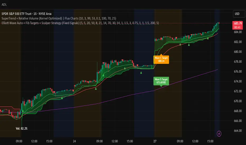
Elliott Wave Auto + Fib Targets + Scalper Strategy (Fixed)// Elliott Wave Auto + Fib Targets + Scalper Strategy
//
// Fixed by expert trader:
// - Replaced table with label-based visualization to avoid 'Column 2 is out of table bounds' error.
// - Uses label.new to display buy/sell signal counts in top-right corner, mimicking table layout.
// - Fixed array.sum() error: Replaced invalid range-based array.sum() with custom sum_array_range() function.
// - Removed barstate usage to fix 'Undeclared identifier barstate' error.
// - Replaced barstate.isconfirmed with true (process every bar).
// - Replaced barstate.isfirstconfirmed with bar_index == 0 (first bar).
// - Replaced strategy.alert with label.new for long/short entry signals (buy/sell markers).
// - Fixed array index out-of-bounds: Protected array.get() calls with size checks.
// - Fixed pyramiding: Set constant pyramiding=4 (max 5 entries); use allow_pyramiding to limit entries.
// - Fixed default_qty_value: Set constant default_qty_value=100.0; use entry_size_pct to scale qty.
// - Replaced alertcondition with labels for Elliott Wave patterns.
// - Fixed partial exits: 50% at TP1 with fixed SL, 50% at TP2 with fixed SL or trailing.
// - Fixed Elliott Wave pivot indexing for alternating H/L check.
// - Ensured proper position sizing and exit logic.
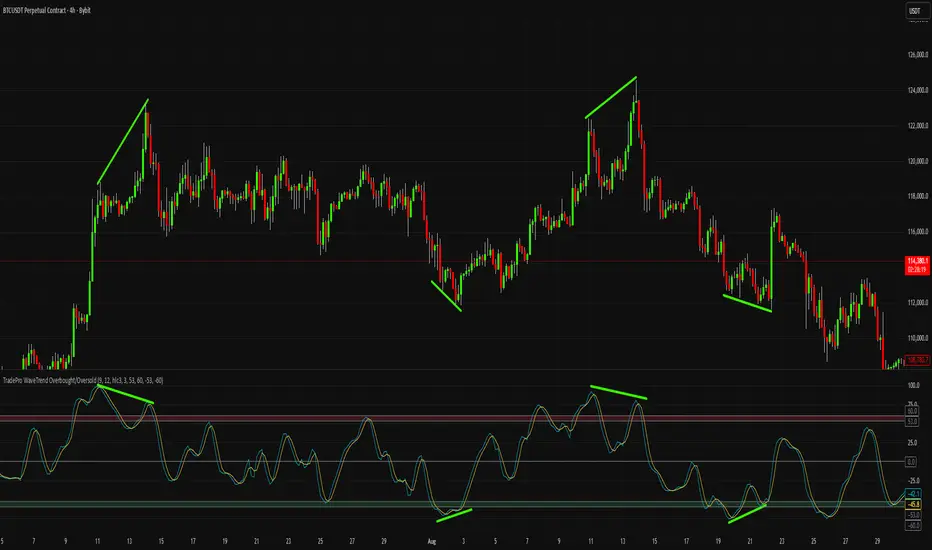
Simplified Wave Trend Overbought/OversoldThis is just a variation of the popular wave trend that I find to be nicer to look at.
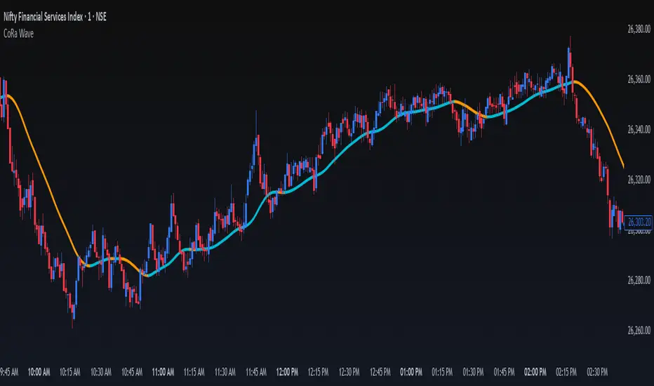
ConeWave MACoRa Wave is a custom-weighted moving average designed to adapt intelligently to market dynamics. It builds upon the foundational logic of the Comp_Ratio_MA by @redktrader, incorporating a compound ratio-based weighting curve that emphasizes recent price action while preserving smoothness and structure with pinescript version 6.
This version introduces modular enhancements, including:
A Comp Ratio Multiplier for fine-tuned responsiveness
Optional Auto Smoothing based on wave length
Streamlined plotting for clarity and performance
Whether you're confirming market structure, identifying trend shifts, or seeking a cleaner alternative to noisy indicators, CoRa Wave offers a visually intuitive and mathematically elegant solution.
🛠 Reimagined by @atulgalande75 — optimized for traders who value precision, adaptability, and clean charting. Original concept by @redktrader.
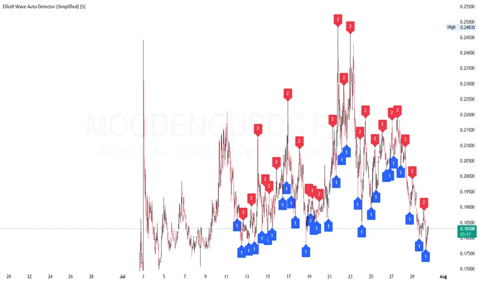
Elliott Wave Auto Detector (Simplified)How to Use the Detector
Identify Structure: Look for sequences like 1-2-1-2...
These may show a forming or ongoing Elliott wave pattern.
Validate Trend: Multiple red 2’s at lower highs suggests a bearish trend; the reverse with blue 1’s at higher lows is bullish.
Trading Zones:
Consider buying near clusters of blue 1’s (support zones).
Consider selling or shorting near clusters of red 2’s (resistance zones).
Look for Breakouts: If price breaks out of the descending channel, trend may reverse or accelerate.
Global M2 Money Supply Top20 + Offset & WaveThe M2 Top20 is a global aggregation of the M2 money supply from the 20 largest economies in the world , providing a comprehensive view of the total liquidity in the global financial system. It is expressed in trillions of USD.
This script calculates and visualizes the M2 Money Supply of the Top 20 Global Economies, adjusted to various timeframes (4H, 1D, 1W, 1M) with customizable offset adjustments (in days) from -1000 days to +1000 days. This indicator includes data from the Americas, Europe, Africa, and the Asia Middle East , offering a diverse and balanced representation of major economic regions. The M2 of each country has been converted to USD.
Additionally, the user can set a minimum and maximum offset to create a wave around the main offset and expand the comparison.
Combining these options, this indicator enables users to visualize a range of the global money supply, making it useful for market analysis, economic forecasting, and understanding macroeconomic trends. This indicator is particularly valuable for traders and analysts interested in understanding the dynamics of global monetary systems and their potential impact on financial markets.
Key Features:
Global M2 Money Supply calculation from the Top 20 Economies.
Adjustable Offset: Adjust the offset to align the indicator with the best bar. Adjustment in days, usable on different timeframes (1D, 1W, 4H, 1M).
Wave Projection: Displays a "probability cloud"—a smoothed area that shows the probable path of Bitcoin, derived from shifts in global liquidity.
Min/Max Offset Adjustments: Customizable offsets allow you to determine the range of future windows, helping to shape the wave and better identify liquidity-driven turning points.
Use Cases:
Economic Forecasting: Identify trends in global money supply and their potential market impact (e.g., historically leads Bitcoin price by +/- 78 days to +/-108 days).
Market Analysis: Track the growth or contraction of money supply across key economies.
Macro-Economic Analysis: Understand the relationship between monetary policies and market performance.
How to use:
Add the indicator to your chart.
Set the timeframe to 1D to customize the offset.
Set the Offset (in days).
Set the Offset Range Minimum and Maximum.
Show/Hide the Range Wave
.
Use offset = 0 to have the indicator align directly with the current data, without any shift, providing a baseline for comparison with the most recent market conditions.
Countries included in the M2 Top20:
China (CN), Japan (JP), South Korea (KR), Hong Kong (HK), Taiwan (TW), India (IN), Saudi Arabia (SA), Thailand (TH), Vietnam (VN), United Arab Emirates (AE), Malawi (MW) – Africa, United States (US), Canada (CA), Brazil (BR), Mexico (MX), Eurozone (EU), United Kingdom (GB), Russia (RU), Poland (PL), Switzerland (CH).
These countries were selected from the ranking of the World Economy Indicator of Trading View .

M2 Liqudity WaveGlobal Liquidity Wave Indicator (M2-Based)
The Global Liquidity Wave Indicator is designed to track and visualize the impact of global M2 liquidity on risk assets—especially those highly correlated to monetary expansion, like Bitcoin, MSTR, and other macro-sensitive equities.
Key features include:
Leading Signal: Historically leads Bitcoin price action by approximately 70 days, offering traders and analysts a forward-looking edge.
Wave-Based Projection: Visualizes a "probability cloud"—a smoothed band representing the most likely trajectory for Bitcoin based on changes in global liquidity.
Min/Max Offset Controls: Adjustable offsets let you define the range of lookahead windows to shape the wave and better capture liquidity-driven inflection points.
Explicit Offset Visualization: Option to manually specify an exact offset to fine-tune the overlay, ideal for testing hypotheses or aligning with macro narratives.
Macro Alignment: Particularly effective for assets with high sensitivity to global monetary policy and liquidity cycles.
This tool is not just a chart overlay—it's a lens into the liquidity engine behind the market, helping anticipate directional bias in advance of price moves.
How to use?
- Enable the indicator for BTCUSD.
- Set Offset Range Start and End to 70 and 115 days
- Set Specific Offset to 78 days (this can change so you'll need to play around)
FAQ
Why a global liquidity wave?
The global liquidity wave accounts for variability in how much global liquidity affects an underlying asset. Think of the Global Liquidity Wave as an area that tracks the most probable path of Bitcoin, MSTR, etc. based on the total global liquidity.
Why the offset?
Global liquidity takes time to make its way into assets such as #Bitcoin, Strategy, etc. and there can be many reasons for that. It's never a specific number of days of offset, which is why a global liquidity wave is helpful in tracking probable paths for highly correlated risk assets.

Renko Momentum Wave (RMW)Renko Momentum Wave
The Renko Momentum Wave (RMW) is a custom momentum oscillator specifically designed for Renko-based price action analysis. Unlike traditional oscillators that rely on time-based data, the RMW focuses on the directional consistency of Renko bricks, measuring the strength of trend momentum purely based on price movement.
Alpha Wave System @DaviddTechAlpha Wave DaviddTech System by DaviddTech is an advanced, meticulously engineered trading indicator adhering strictly to the DaviddTech methodology. Rather than simply combining popular indicators, Alpha Wave strategically integrates specially-selected technical components—each optimized to enhance their combined strengths while neutralizing individual weaknesses, providing traders with clear, consistent, and high-probability trading signals.
Valid Setup:
🎯 Why This Combination Matters:
Quantum Adaptive Moving Average (Baseline):
This advanced adaptive MA provides superior responsiveness to market shifts by dynamically adjusting its sensitivity, clearly indicating the primary market direction and reducing lag compared to standard moving averages.
WavePulse Indicator (CoralChannel-based Confirmation #1):
Precisely detects shifts in momentum and price acceleration, allowing traders to anticipate trend continuation or reversals effectively, significantly enhancing trade accuracy.
Quantum Channel (G-Channel-based Confirmation #2):
Dynamically captures price volatility ranges, offering reliable trend structure validation and clear support/resistance channels, further increasing signal reliability.
Momentum Density (Volatility Filter):
Ensures traders enter only during optimal volatility conditions by quantifying momentum intensity, effectively filtering out low-quality, low-momentum scenarios.
Dynamic ATR-based Trailing Stop (Exit System):
Automatically manages trade exits with optimized ATR-based stop levels, systematically securing profits while effectively managing risk.
These meticulously integrated components reinforce each other's strengths, providing traders with a robust, disciplined, and clearly structured approach aligned with the DaviddTech methodology.
🔥 Latest Update – Enhanced BUY & SELL Signals:
Alpha Wave now clearly displays automated BUY and SELL signals directly on your chart, coupled with a comprehensive dashboard table for immediate signal validation. Signals appear only when all components—including baseline, confirmations, and volatility—are in alignment, significantly improving trade accuracy and confidence.
📌 How Traders Benefit from the New Signals:
BUY Signal: Execute long trades when Quantum Adaptive MA signals bullish, confirmed by bullish WavePulse momentum, bullish Quantum Channel structure, and strong Momentum Density readings.
SELL Signal: Clearly marked for entering short positions under bearish market conditions verified through Quantum Adaptive MA, WavePulse bearish momentum, Quantum Channel confirmation, and sufficient Momentum Density.
Signal Validation: A dedicated dashboard provides immediate visual strength metrics, allowing traders to quickly validate signals before execution, significantly enhancing trading discipline and consistency.
📊 Recommended DaviddTech Trading Plan:
Baseline: Determine overall market direction using Quantum Adaptive MA. Only trade in the indicated baseline direction.
Confirmations: Validate potential entries with WavePulse and Quantum Channel alignment.
Volatility Filter: Confirm sufficient market volatility with Momentum Density before entry.
Trailing Stop Loss: Manage risk and secure profits using the dynamic ATR-based trailing stop system.
Entries & Exits: Only execute trades when signals and dashboard components unanimously align.
🖼️ Visual Examples:
Alpha Wave by DaviddTech clearly demonstrates how an intelligently integrated system provides significantly superior trading insights compared to standalone indicators, ensuring precise, disciplined, and profitable market entries and exits across all trading environments.

[blackcat] L2 Wave Base CampOVERVIEW
The L2 Wave Base Camp indicator is a technical analysis tool designed to identify trends and potential trading signals by visualizing price and volume data through moving averages and relative strength calculations. It operates in its own panel on the trading chart, providing traders with a clear and color-coded representation of market conditions.
FEATURES
Customizable Base Camp Level: Users can set a horizontal line at a specific level to mark significant price points.
Color-Coded Histograms: Different colors indicate various market conditions, such as price position relative to moving averages.
Labeled Signals: The indicator labels potential "Valley" and "Top" points, suggesting buying and selling opportunities.
Volume Analysis: Incorporates volume data to identify potential trend reversals based on volume trends.
HOW TO USE
Set the Base Camp Level: Adjust the input parameter to define a significant price level.
Interpret Histogram Colors: Use the color-coded histograms to understand the current market condition.
Look for Labeled Signals: Pay attention to "Valley" and "Top" labels for potential trading opportunities.
Analyze Volume Trends: Monitor volume data for signs of trend reversals.
LIMITATIONS
Not a Standalone Tool: Should be used in conjunction with other indicators and analysis methods.
Backtesting Required: Essential to understand historical performance before live trading.
NOTES
The indicator uses moving averages (SMA) and relative strength calculations to smooth data and identify trends.
Crossover events between different moving averages generate buy and sell signals.
THANKS
Special thanks to the original author for developing this insightful trading tool.

[blackat] L1 Funding Bottom Wave█ OVERVIEW
The script "Funding Bottom Wave" is an indicator designed to analyze market conditions based on multiple smoothed price calculations and specific thresholds. It calculates several values such as B-value, VAR2-value, and additional signals like SK and SD to identify buy/sell levels and reversals, aiding traders in making informed decisions.
█ LOGICAL FRAMEWORK
The script consists of several main components:
• Input parameters that allow customization of calculation periods and thresholds.
• A custom function funding_wave that computes various financial metrics and conditions.
• Plotting commands to visualize different aspects of those computations.
Data flows from input parameters into the funding_wave function where calculations are performed. These results are then plotted according to specified conditions. The script uses conditional expressions to define when certain plots should appear based on the computed values.
█ CUSTOM FUNCTIONS
funding_wave Function:
This function takes six arguments: close_price, high_price, low_price, open_price, period_b, and period_var2. It performs several calculations including:
• Price range percentage normalized between lowest and highest prices over 60 bars.
• SMA of this value over periods defined by period_b and period_var2.
• Several moving averages (MA), EMAs, and extreme point markers (highest/lowest).
• Multiple condition checks involving these metrics leading to buy/high signal flags.
Returns: An array containing B-value, VAR2-value, SK-value, SD-value, along with various conditional signal indicators.
█ KEY POINTS AND TECHNIQUES
• Utilizes built-in TA functions (ta.highest, ta.lowest, ta.sma, ta.ema) for smoothing and normalization purposes.
• Implements extensive use of ternary operators and boolean logic to determine plot visibility based on specific criteria.
• Employs column-style plotting which highlights significant transitions in calculated metric levels visually.
• No explicit loops; computations utilize vectorized operations inherent to Pine Script's nature.
█ EXTENDED KNOWLEDGE AND APPLICATIONS
Potential modifications/extensions include:
• Adding alerts for key threshold crossovers or meeting certain conditions.
• Customizing more sophisticated alert messages incorporating current time and symbol details.
• Incorporating stop-loss/take-profit strategies dynamically adjusted by indicator outputs.
Similar techniques can be applied in:
• Developing robust trend-following systems combining momentum oscillators.
• Enhancing basic price action rulesets with statistical filters derived from historical data behaviors.
• Exploring intraday breakout strategies predicated upon sudden changes in market sentiment captured via volatility spikes.
Related concepts/features:
• Using arrays to encapsulate complex return structures for reusability across scripts/functions.
• Leveraging na effectively within plotting constructs ensures cleaner chart presentation avoiding clutter from irrelevant points.
█ MARKET MEANING OF DIFFERENT COLORED COLUMNS
Red Columns ("B above Var2"):
• Market Interpretation: When the red columns appear, it indicates that the B-value is higher than the VAR2-value. This suggests a strengthening upward trend or consolidation phase where the market might be experiencing buying pressure relative to recent trends.
• Trading Implication: Traders may consider this as a potentially bullish sign, indicating strength in the underlying asset.
Green Columns ("B below Var2"):
• Market Interpretation: Green columns indicate that the B-value is lower than the VAR2-value. This could suggest downward trend acceleration or weakening buying pressure compared to recent trends.
• Trading Implication: Traders might interpret this as a bearish signal, suggesting a possible decline in the market.
Aqua Columns ("SK below SD"):
• Market Interpretation: Aqua columns show instances where the SK-value is below the SD-value. This typically signifies that the short-term stochastic oscillator (or similar measure) is signaling oversold conditions but not yet reaching extremes.
• Trading Implication: While not necessarily a strong sell signal, aqua columns might prompt traders to look for further confirmation before entering long positions.
Fuchsia Columns ("SK above SD"):
• Market Interpretation: Fuchsia columns represent situations where the SK-value exceeds the SD-value. This usually indicates overbought conditions in the near term.
• Trading Implication: Traders often view fuchsia columns as cautionary signs, possibly prompting them to exit existing long positions or refrain from adding new ones without further analysis.
Yellow Columns ("High Condition" and "High Condition Both"):
• Market Interpretation: Yellow columns occur when either the SK-value or B-value crosses above predefined high thresholds (e.g., 90). If both cross simultaneously, they form "High Condition Both."
• Trading Implication: Strongly bullish signals indicating overheated markets prone to corrections. Traders may see this as a good opportunity to take profits or prepare for a pullback/corrective move.
Blue Columns ("Low Condition" and "Low Condition Both"):
• Market Interpretation: Blue columns emerge when either the SK-value or B-value drops below predefined low thresholds (e.g., 10). Simultaneous crossing forms "Low Condition Both."
• Trading Implication: Potentially bullish reversal setups once the market starts showing signs of bottoming out after being significantly oversold. Traders might use blue columns as entry points for establishing long positions or hedging against anticipated rebounds.
Light Purple Columns ("Low Condition with Reversal" and "Low Condition Both with Reversal"):
• Market Interpretation: Light purple columns signify moments when the SK-value or B-value falls below their respective thresholds but has started reversing upwards immediately afterward. If both fall and reverse together, it's denoted as "Low Condition Both with Reversal."
• Trading Implication: Suggests a possible early-stage rebound from an extended downtrend or sideways movement. This could be seen as a highly reliable bulls' flag formation setup.
White Columns ("High Condition with Reversal" and "High Condition Both with Reversal"):
• Market Interpretation: White columns denote scenarios where the SK-value or B-value breaches high thresholds (e.g., 90) but begins descending shortly thereafter. Both simultaneously crossing leads to "High Condition Both with Reversal."
• Trading Implication: Indicative of peak overbought conditions followed quickly by exhaustion in buying interest. This warns traders about potential imminent retracements or pullbacks, prompting exits or short positions.
█ SUMMARY TABLE OF COLUMN COLORS AND THEIR MEANINGS
Color Type Market Interpretation Trading Implication
Red B above Var2 Strengthening upward trend/consolidation Bullish sign
Green B below Var2 Downward trend acceleration/weakening buying pressure Bearish sign
Aqua SK below SD Oversold conditions but not extreme Cautionary signal
Fuchsia SK above SD Overbought conditions Take profit/precaution
Yellow High Condition / High Condition Both Overheated market, likely correction coming Good time to exit/additional selling
Blue Low Condition / Low Condition Both Possible bull/rebound setup Entry point/hedging
Light Purple Low Condition with Reversal / Low Condition Both with Reversal Early-stage rebound from downtrend Reliable bulls' flag formation
White High Condition with Reversal / High Condition Both with Reversal Peak overbought with imminent retracement Exit positions/warning
Understanding these color-coded signals can help traders make more informed decisions, whether for entry, exit, or risk management in trading strategies. Each set of colors provides distinct insights into market dynamics and trends, aiding in effective execution of trade plans.

Prometheus Fractal WaveThe Fractal Wave is an indicator that uses a fractal analysis to determine where reversals may happen. This is done through a Fractal process, making sure a price point is in a certain set and then getting a Distance metric.
Calculation:
A bullish Fractal is defined by the current bar’s high being less than the last bar’s high, and the last bar’s high being greater than the second to last bar’s high, and the last bar’s high being greater than the third to last bar’s high.
A bearish Fractal is defined by the current low being greater than the last bar’s low, and the last bar’s low being less than the second to last bar’s low, and the last bar’s low being less than the third to last bar’s low.
When there is that bullish or bearish fractal the value we store is either the last bar’s high or low respective to bullish or bearish fractal.
Once we have that value stored we either subtract the last bar’s low from the bullish Fractal value, and subtract the last bar’s high from the bearish Fractal value. Those are our Distances.
Code:
isBullishFractal() =>
high > high and high < high and high > high
isBearishFractal() =>
low < low and low > low and low < low
var float lastBullishFractal = na
var float lastBearishFractal = na
if isBullishFractal() and barstate.isconfirmed
lastBullishFractal := high
if isBearishFractal() and barstate.isconfirmed
lastBearishFractal := low
//------------------------------
//-------CACLULATION------------
//------------------------------
bullWaveDistance = na(lastBullishFractal) ? na : lastBullishFractal - low
bearWaveDistance = na(lastBearishFractal) ? na : high - lastBearishFractal
We then plot the bullish distance and the negative bearish distance.
The trade scenarios come from when one breaks the zero line and then goes back above or below. So if the last bullish distance was below 0 and is now above, or if the last negative bearish distance was above 0 and now below. We plot a green label below a candle for a bullish scenario, or a red label above a candle for a bearish one, you can turn them on or off.
Code:
plot(bullWaveDistance, color=color.green, title="Bull Wave Distance", linewidth=2)
plot(-bearWaveDistance, color=color.red, title="Bear Wave Distance", linewidth=2)
plot(0, "Zero Line", color=color.gray, display = display.pane)
bearish_reversal = plot_labels ? bullWaveDistance < 0 and bullWaveDistance > 0 : na
bullish_reversal = plot_labels ? -bearWaveDistance > 0 and -bearWaveDistance < 0 : na
plotshape(bullish_reversal, location=location.belowbar, color=color.green, style=shape.labelup, title="Bullish Fractal", text="↑", display = display.all - display.status_line, force_overlay = true)
plotshape(bearish_reversal, location=location.abovebar, color=color.red, style=shape.labeldown, title="Bearish Fractal", text="↓", display = display.all - display.status_line, force_overlay = true)
We can see in this daily NASDAQ:QQQ chart that the indicator gives us marks that can either be used as Reversal signals or as breathers in the trend.
Since it is designed to provide reversals, on something like Gold where the uptrend has been strong, the signals may be just short breathers, not full blown strong reversal signs.
The indicator works just as well intra day as it does on larger timeframes.
We encourage traders to not follow indicators blindly, none are 100% accurate. Please comment on any desired updates, all criticism is welcome!

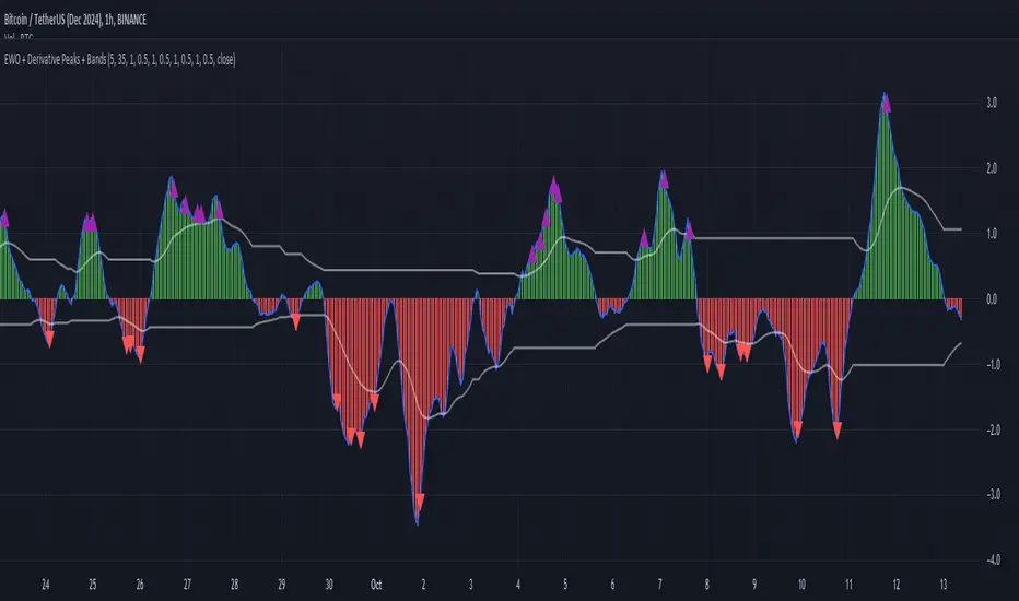
Elliott Wave Oscillator with Peak DetectionThe Elliott Wave Oscillator with Derivative Peak Detection and Breakout Bands is a technical indicator that blends traditional Elliott Wave theory with modern derivative-based peak detection and breakout bands for a clearer view of market trends.
Key Components:
Elliott Wave Oscillator (EWO):
The core of the indicator is based on the difference between two simple moving averages (SMA): a short-term SMA (default length: 5) and a long-term SMA (default length: 35).
This difference is expressed either as an absolute value or a percentage of the current price, depending on the user’s input.
Smoothing:
The EWO is smoothed using an Exponential Moving Average (EMA) to filter out noise and provide a clearer trend direction.
The smoothing length is adaptive based on the current chart's timeframe (e.g., longer smoothing for daily charts).
Derivative Peak Detection:
The smoothed EWO is analyzed for peaks (positive) and troughs (negative) by calculating the derivative (rate of change) between consecutive values.
Peaks are detected when the derivative transitions from positive to negative, while troughs are identified when the derivative switches from negative to positive.
Tolerance levels are adjustable and vary by timeframe to avoid false signals.
Breakout Bands:
Upper and lower breakout bands are dynamically generated based on the smoothed EWO.
The bands help to filter significant peaks and troughs, only highlighting those that occur beyond the breakout levels.
Users can choose to display these bands and use them to filter out less significant peaks and troughs.
Visualization:
The original, unsmoothed EWO is plotted as a histogram, with positive values in green and negative values in red.
The smoothed EWO is plotted as a blue line, providing a clearer view of the underlying trend.
The breakout bands, if enabled, are plotted as white lines to visualize the upper and lower bounds of the oscillator's movement.
Positive peaks and negative troughs that meet the filtering criteria are marked with purple triangles (for peaks) and red triangles (for troughs) on the chart.
Customization Options:
Timeframe-based Smoothing and Tolerance: Different smoothing lengths and tolerance levels can be set for daily, hourly, and 5-minute charts.
Breakout Bands: Users can toggle the display of breakout bands and adjust their visual properties.
Peak Filtering: Peaks and troughs can be filtered based on whether they break out beyond the bands, or all peaks can be shown.
This indicator provides a unique blend of trend detection through the Elliott Wave Oscillator and derivative analysis to highlight significant market reversals while offering breakout bands as a filtering mechanism for false signals.
T-Wave Pattern IdentifierA T-wave might describe a pattern where the price movement forms a "T" shape on the chart, which could involve:
Strong Vertical Movement (The Stem of the T):
This could represent a sharp, decisive move in one direction (up or down), often occurring in a single candle or a few candles. This movement could be seen as the "stem" of the T.
For example, a sudden spike up in price followed by a horizontal consolidation.
Horizontal Movement (The Cross of the T):
Following the sharp move, the price might consolidate sideways, forming a horizontal base or resistance/support level, which creates the top cross of the "T."
This could indicate a pause or a consolidation phase after a significant move, where the price moves within a narrow range.
Contexts Where a T-Wave Pattern Might Be Useful:
Breakout Scenarios: If a T-wave forms after a significant upward or downward movement, it could suggest a potential continuation in the direction of the initial move, especially if the price breaks out of the consolidation range.
Reversal Signals: Alternatively, the T-wave could act as a reversal pattern if the price fails to continue in the direction of the initial move and instead breaks out in the opposite direction.
T-Wave Logic Example:
Stem (Vertical Movement):
Identify a candle or series of candles with a significant price move (e.g., a large-bodied candle with a relatively small wick). This shows momentum in one direction.
Cross (Horizontal Movement):
Following the vertical move, identify a consolidation phase where the price moves sideways in a relatively tight range. This could be visualized as a series of small candles with overlapping highs and lows.

Bitcoin Wave RainbowThis Bitcoin Wave Rainbow model is a powerful tool designed to help traders of all levels understand and navigate the Bitcoin market. It works only with BTC in any timeframe, but better looks in dayly or weekly timeframes. It provides valuable insights into historical price behavior and offers forecasts for the next decade, making it an essential asset for both short-term and long-term strategies.
How the Model Works
The model is built on a logarithmic trend, also known as a power law, represented by the green line on the chart. This line illustrates the expected price trajectory of Bitcoin over time. The model also incorporates a range of price fluctuations around this trend, represented by colored bands.
The width of these bands narrows over time, indicating that the model becomes increasingly accurate as it progresses. This is due to the exponential decrease in the range of price fluctuations, making the model a reliable tool for predicting future price movements.
Understanding the Zones
Blue Zone: This zone signifies that the price is below its trend, making it a recommended area for buying Bitcoin. It represents a level where the price is unlikely to fall further, providing a potential opportunity for accumulation.
Green Zone: This zone represents a fair price range, where the price is relatively close to its trend. In this zone, the price may continue to go up or down, depending on the halving season. ransiting up around any halving and transiting down around 2 years after each halving.
Yellow Zone: This zone indicates that the price is somewhat overheated, often due to the hype following a halving event. While there may still be room for the price to rise, traders should exercise caution in this zone, as a price correction could occur.
Red Zone: This zone represents a strong overbought condition, where the price is significantly above its trend. Traders should be extremely cautious in this zone and consider reducing their positions, as the price is likely to revert back towards the trend or even lower.
Using the Model in Your Trading Strategy
This indicator can be used in conjunction with the Bitcoin Wave Model, which complements it by showing harmonic price fluctuations associated with halving events. Together, these indicators provide a comprehensive view of the Bitcoin market, allowing traders to make informed decisions based on both historical data and future projections.
Benefits for Traders
This Bitcoin price model offers numerous benefits for traders, including:
Clear Visualization: The model provides a clear and concise visual representation of Bitcoin's price behavior, making it easy to understand and interpret.
Accurate Forecasting: The model's accuracy increases over time, providing reliable forecasts for future price movements.
Risk Management: The model helps traders identify overbought and oversold conditions, allowing them to manage their risk more effectively.
Strategic Decision-Making: By understanding the different zones and their implications, traders can make more informed decisions about when to buy, sell, or hold Bitcoin.
By incorporating this Bitcoin price model into your trading strategy, you can gain a deeper understanding of the market dynamics and improve your chances of success.

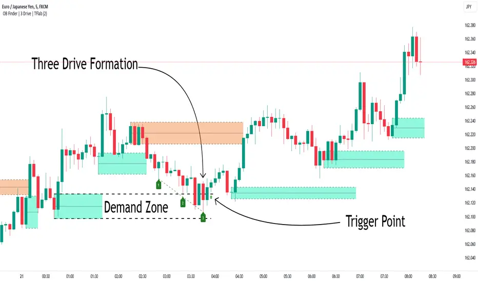
Smart Money Setup 04 [TradingFinder] Three Drive (Harmonic) + OB🔵 Introduction
The "Three Drive" pattern is a well-known formation in technical analysis, recognized for its ability to signal potential trend reversals in price action. Within the realm of trading, particularly in the context of "Reversal Patterns," the Three Drive pattern holds significance as a reliable indicator of shifts in market sentiment.
🟣 Bullish 3 Drive
This pattern typically manifests at a price bottom, where a sequence of lower lows suggests a prevailing negative trend. However, within the structure of the Three Drive pattern, a notable occurrence unfolds.
The second low breaches the range of the first low, followed by the third low surpassing the range of the second low. These penetrations signify a diminishing selling pressure and an emerging buying interest.
Traders often await the confirmation of the third low surpassing the second low as an entry point, with price targets set at the highs formed within the Three Drive pattern.
🟣 Bearish 3 Drive
Conversely, the Bearish Three Drive pattern emerges at a price top, characterized by a sequence of higher highs indicating an upward trend. Yet, amidst this apparent bullish momentum, a shift occurs.
The second high breaks beyond the range of the first high, succeeded by the third high exceeding the range of the second high. These breaches signify a waning buying strength and a resurgence in selling pressure.
Entry into a trade is often executed after the confirmation of the third high surpassing the second high, with targets set at the lows formed within the Three Drive pattern.
Importance :
Understanding the Three Drive pattern's significance extends beyond mere technical analysis. It bears resemblance to other established patterns, such as the Harmonic Pattern and Ending Diagonal within the Elliott Wave Theory.
Recognizing these parallels aids traders in comprehending broader market dynamics and potential price movements.
🔵 Formation of 3 Drive in Order Block Zone
The convergence of the Three Drive pattern with the concept of the Order Block Zone introduces a nuanced layer to traders' analytical approach.
In "Price Action" methodology, Order Blocks represent areas on the price chart where significant market players, such as institutional traders, have executed notable orders.
These zones often act as barriers, with price encountering resistance or support upon reaching them.
When the Three Drive pattern forms within an Order Block Zone, it signifies a confluence of market dynamics.
The completion of the pattern within this zone suggests a potential reversal in the prevailing trend, augmented by the presence of significant institutional orders.
Traders incorporate these Order Blocks into their analysis to identify probable levels where price may change direction, enhancing the reliability of their trading decisions.
🔵 How to Use :
To effectively utilize the Three Drive pattern within the Order Block Zone, traders seek alignment between the completion of the pattern and the presence of significant Order Blocks.
This convergence enhances the reliability of the pattern's signals, increasing the likelihood of successful trade outcomes.
Bullish Three Drive in Demand Zone :
Bearish Three Drive in Supply Zone :
Settings :
You can set your desired "Pivot Period" via settings for the indicator to identify setups based on it.
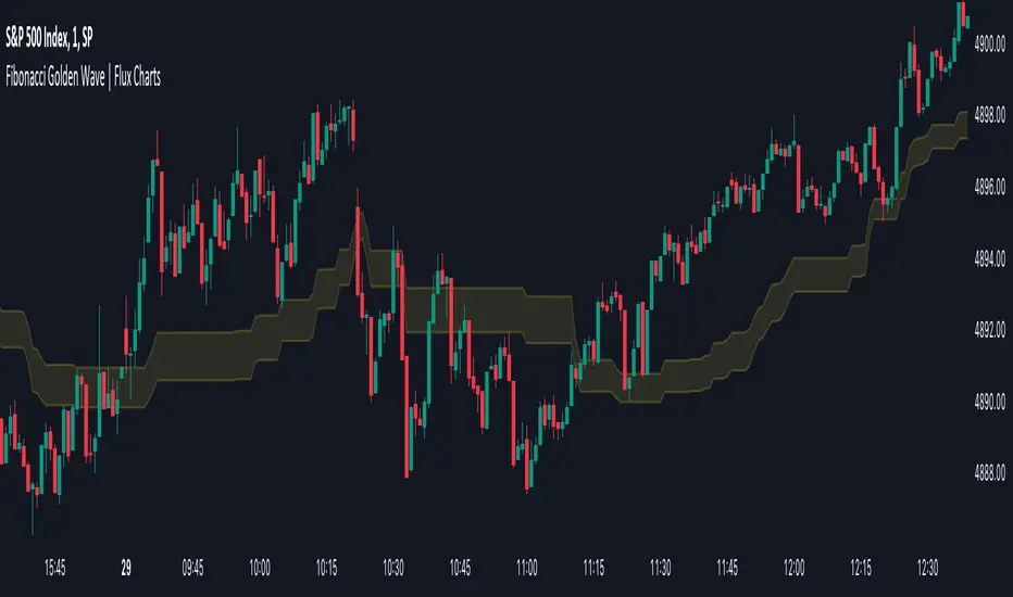
Fibonacci Golden Wave | Flux Charts💎 GENERAL OVERVIEW
Introducing the new Fibonacci Golden Wave indicator! This indicator plots the Fibonacci golden zone from the last highs / lows instead of the pivots so that the resulting zone is shaped like a "wave". We believe this will help you to see the latest trend of the Fibonacci retracement levels easier. For more information of the working progress of the indicator, check the "How Does It Work" section of the description.
Features of the new Fibonacci Golden Wave Indicator :
Plots Fibonacci Golden Zone Based On Highs / Lows
A Different Approach To Fibonacci Retracement Levels
Customizable Swing Range & Retracement Levels
Customizable Visuals
🚩UNIQUENESS
The Fibonacci Golden Zone is a widely used concept in trading. To achieve the golden zone, the Fibonacci retracement levels are generally placed between pivot high / lows, resulting in a rectangular zone. However, this indicator will place the Fibonacci retracement levels between the last highest / lowest points going back from the current bar, resulting in a "wave" shape. This will help traders understand the latest trend of the Fibonacci golden zone. The ability to change the Fibonacci retracement levels to your liking in the settings is another unique function of this indicator.
📌 HOW DOES IT WORK ?
To calculate the Fibonacci wave, first of all we need to place a line at the lowest low and the highest high of the last 20 bars (can be changed from the settings)
Then, Fibonacci retracement levels are placed between those lines.
For the next step, put two points in the (1.0 - 0.618) = 0.382 and (1.0 - 0.5) = 0.5 (can be changed from the settings) levels of the Fibonacci retracement.
Repeat this step for each bar in the chart, then connect all the points.
Instead of a pivot approach to the Fibonacci retracement levels, this approach will not need a new pivot point to form before calculating the new Fibonacci golden zone, thus indicating the latest trend of the current golden zone.
🚨HOW YOU CAN USE THIS INDICATOR
Fibonacci retracement tool is typically used to find entries after a pullback in an uptrend or downtrend. The Fibonacci Golden Wave can be used in the same way. It can be used to find entries after markets retrace. In this example, the Fibonacci Golden Wave is able to catch 2 pullback opportunities to enter long in the market with the trend.
⚙️SETTINGS
1. General Configuration
Swing Range -> This setting determines how the highest high / lowest low levels are calculated. This essentially means that the script will look back X bars before the current bar in calculation to find the highest / lowest wick points.
2. Golden Zone
Here you can select which range of the Fibonacci retracement levels should be considered as the golden zone. The default value is 0.5 - 0.618.
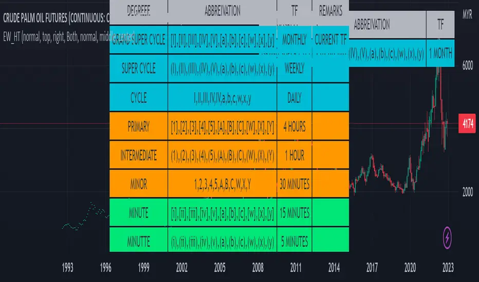
Elliot Wave Helper Table█ OVERVIEW
This indicator is intend to be helper to help Elliot Wave user to properly Elliot Wave tools according to correct degree such as 12345 or ABCWXY. The abbreviation changes according to timeframe.
█ FEATURES
1. Abbreviation degree adaptive to timeframe. Eg : Subminutte for 1 minute chart, etc.
2. Works for custom timeframe. Eg : Subminutte for 1 to 4 minute chart, etc.
3. Show reference table if necessary.
█ REFERENCE
Adaptive Elliot Wave Degree Chart
█ EXAMPLES / USAGES