ALMA Smoothed Gaussian Moving AverageThis indicator is an altered version of the Gaussian Moving Average (GMA) (Credit to author: © LeafAlgo ). The GMA applies weights to the prices, giving more importance to the values closer to the current period and gradually diminishing the significance of older prices. The ALMA Smoothed Gaussian Moving Average (ASGMA) applies an ALMA smoothing to its price data to minimize lag and provide a more accurate representation of the underlying trend by dynamically adapting to changing market conditions. The Arnaud Legoux Moving Average (ALMA) is a specialized smoothing technique that adjusts the weights of the moving average based on market volatility. Its calculation uses Wavelet Transform techniques which enables this type of smoothing to capture both high-frequency and low-frequency components of a signal or data. The rationale for this mashup between ALMA and Gaussian filtering is to smooth the moving average line over the smoothed price data and produce stronger trend signals.
ASGMA serves as a trend-following indicator, identifying both bullish and bearish trends. It provides buy and sell signals indicated by "B" and "S" labels plotted alongside the price data. Additionally, the ASGMA's Exponential Moving Average (EMA) line alternates between green and red, indicating bullish and bearish momentum, respectively.
The ASGMA also incorporates two popular momentum indicators, the Relative Strength Index (RSI) and the Chande Momentum Oscillator (CMO). The inclusion of these indicators aims to enhance trend identification and reversal signals. For a strong buy signal, all three indicators (RSI, CMO, and ASGMA) must indicate bullish conditions, resulting in a vertical green line. Conversely, a vertical red line is plotted when all indicators indicate bearish conditions, representing a strong sell signal.
The ASGMA, with its unique combination of smoothing techniques and indicator amalgamation, provides traders and investors with powerful analytical tools. It can be applied in trend-following strategies using the regular buy and sell signals generated by labels and the EMA line. Alternatively, the vertical lines offer stronger buy and sell signals. These features aid in identifying potential entry and exit points, thereby enhancing trading decisions and market analysis. However, it is important to remember that the future performance of any trading strategy is fundamentally unknowable, and past results do not guarantee future performance.
Cerca negli script per "wave"

Planetary Tunings Moving AveragesThe Pine Script "Planetary Tunings Moving Averages" is a unique tool that plots moving averages (MAs) on a chart, representing the wavelengths of different planets as derived from the book Quadrivium. These wavelengths, also referred to as 'planetary tunings', are related to the orbital resonance of each planet.
Each planetary tuning value is first transformed into a whole number by multiplying it by 1000 and removing the decimal. This whole number is then used as the length parameter for a Simple Moving Average (SMA) function. This function calculates the average of the closing prices over the defined number of periods, thereby creating a moving average line on the chart.
The moving average lines are color-coded according to the planet they represent, allowing for quick and easy interpretation. For example, Mercury's moving average line is blue, Venus's line is orange, and so forth. These colors can be adjusted directly in the Pine Script code if desired.
Additionally, the script computes the mean of all these moving averages and plots it on the chart. This line provides an overall trend line, summarizing the collective behavior of all the planetary tuning moving averages.
The drawings in the chart are fib channels and fib circles that I use to capture liquidity in time.
Please note that this script is written for Pine Script Version 4. It's crucial to ensure your TradingView platform is compatible with this version. For any issues or further clarification, consider referring to TradingView's Pine Script documentation or its community forums.

RHODL_RatioIndicator Overview
This indicator uses a ratio of Realized Value HODL Waves.
In summary, Realized Value HODL waves are different age bands of UTXO’s (coins) weighted by the Realized Value of coins within each band.
The Realized Value is the price of UTXO’s (coins) when they were last moved from one wallet to another.
RHODL Ratio looks at the ratio between RHODL band of 1 week versus the RHODL band of 1-2yrs.
It also calibrates for increased hodl’ing over time and for lost coins by multiplying the ratio by the age of the market in number of days.
When the 1-week value is significantly higher than the 1-2yr it is a signal that the market is becoming overheated.
How to Use this Indicator
When RHODL ratio starts to approach the red band it can signal that the market is overheating (Red bars on a chart). This has historically been a good time for investors to take profits in each cycle.
When RHODL ratio starts to approach the green band it can signal great time to buy (Green bars on a chart)
If you change an upper band location this automatically affects on the normalization of value what you can send with allert and what you see on the lable.
This version have differences to original one
Original idea of:
Philip Swift (@positivecrypto)

Volatility Percentile (H-LINES)A simple script that adjusts the Volatility Percentile Indicator visibly in order to better accommodate entries/exits and certain trading setups/strategies.
--------------------------------------------------------------------------------------------------------------------------------------------------------
TL;DR - Remember after a full reset, we are looking for initial crosses UP on the UpperSwingline and crosses DOWN on the LowerSwingline for primary and secondary signal derivation.
Vice versa also works great but the prior method mentioned is a little more consistent in my experience, but you should mess around and optimise this for your own setups and strategies anyway.
--------------------------------------------------------------------------------------------------------------------------------------------------------
ORIGINAL SCRIPT HERE:
^Click image for a redirect to that script.
ALL CREDIT GOES TO: www.tradingview.com
He wrote everything so give credit where it's due, good bit of kit this here script is.
--------------------------------------------------------------------------------------------------------------------------------------------------------
HOW I USE MY VISUALLY ALTERED VERSION OF THIS SCRIPT
First of all, the alterations I've made seem only to be consistently viable with renko charts though if you can get the sought after results using candles or any other chart type then perfect, but be wary. All my back-testing done only with LinReg, HMA and SWMA - ATR type settings exclusively on renko charts. The changes I've made to the original script essentially just turns it visibly into an oscillator and uses a couple horizontal lines to generate signals, very simple - absolutely nothing has changed in the actual code of calculating this indicator.
What I believe my adjustments have achieved is quite simple. A full reset/oscillation on the indicator tries to map the strongest parts of a move or at least the part of the move where volume and the rate of transactions is at its peak to even facilitate said move. *take this statement with a pinch of salt though I do believe it's interacting with accumulation/distribution patterns, which is expected of volatility*
For ease of communication let's refer to the area between the the first UpperSwingline cross to the subsequent LowerSwingline cross, as the primary move. Then afterwards when it crosses the UpperSwingline again to make the full reset, the area in between those two points referred to as the secondary move.
Though more interestingly/practically the indicator ends up giving you two signals. In order for this to work we have to first decide that a spike up in volatility which crosses the UpperSwingline implies a significant level of interest at that price level. Usually that means a reversal is brewing, if price has already moved, trended and is approaching a certain area of value; which causes a spike of new positions to be taken, then you know that this is a level where contrarians are looking to enter. Now here's the tricky part, when volatility crosses the LowerSwingline price action becomes a little more open for interpretation, the way I personally like to look at this secondary signal is the potential for an exhaustion period to prolong itself a little longer. I know that's not the perfect analysis for what's going on, a more in-depth look into what's going on would best be described using Elliott Wave Theory, if a cross on the UpperSwingline near a significant area of value gives us a reversal trade lets just assume for the sake of argument that a new Elliott Wave can begin forming here. Making the move from that initial UpperSwngline cross to the cross on the LowerSwingline, the area that encompasses those two points: the impulse wave. After this point my analogy kind of falls apart and sadly my knowledge just isn't what it needs to be in order for me to properly analyse what's going on here but I must digress. Price after crossing the LowerSwingline up until the point where it makes a full reset by crossing the UpperSwingline again, within this area price seems to do either one of two things:
Situation 1 - Most likely occurs after a major trend reversal from major support/resistance or area of value (price has trended to new territory, maybe spent time a little time consolidating but hasn't broken the key level, momentum shifts, price action breaks current structure and you get the signal that primary move is a reversal) = Exhaustion Period, price will continue in direction of primary move during the secondary move. This here is for our trend-followers, you wanna take a continuation trade? Just wait for the pullback/rally to hit a FiB retracement level and enter - or any other means to find a decent support/resistance to enter.
Situation 2 - Most likely occurs when market enters a range or consolidation (price was previously seen as being at either a discount or premium so Situation 1 could have already played out and now you're looking at a full reset after that, imagine this spot to be the centre line of a linear regression channel or bang in the middle of your range, could even occur if price breaks a key moving average and decides it ought to consolidate around it for a while. Basically at any point where a somewhat prolonged consolidation is expected and not a quick reversal) = Corrective Wave, price will move against the direction of primary move during the secondary move. Now you might be expecting me to say this ones for you reversal traders but not really, if this is occurring then there probably isn't a definitive direction the market has chosen so you can use this opportunity to take range trades in the direction or against the direction of whatever the current trend or latest trend was depending on whatever slight bias you may have. <--- Situation 2 is very useful for finding cleaner entries if you do have a trend bias, say price underwent Situation 1, is now at key moving average but your bias is that it will break and continue up, so you wait and allow the secondary move of Situation 2 to take your entry to a much better R:R before entering a position.
--------------------------------------------------------------------------------------------------------------------------------------------------------

Hurst Diamond Notation PivotsThis is a fairly simple indicator for diamond notation of past hi/lo pivot points, a common method in Hurst analysis. The diamonds mark the troughs/peaks of each cycle. They are offset by their lookback and thus will not 'paint' until after they happen so anticipate accordingly. Practically, traders can use the average length of past pivot periods to forecast future pivot periods in time🔮. For example, if the average/dominant number of bars in an 80-bar pivot point period/cycle is 76, then a trader might forecast that the next pivot could occur 76-ish bars after the last confirmed pivot. The numbers/labels on the y-axis display the cycle length used for pivot detection. This indicator doesn't repaint, but it has a lot of lag; Please use it for forecasting instead of entry signals. This indicator scans for new pivots in the form of a rainbow line and circle; once the hi/lo has happened and the lookback has passed then the pivot will be plotted. The rainbow color per wavelength theme seems to be authentic to Hurst (or modern Hurst software) and has been included as a default.

Overlay - HARSI + Divergences // All credit to © //@author=JayRogers & VuManChu Cipher B for their original Scripts (Open Source)
/ ====== ABOUT THIS INDICATOR
// I've combined some part of the code of the following indicators to get some alerts based on the Idea and Use section below :
// - RSI based Heikin Ashi candle oscillator
// - Divergence based on the VuManChu Cipher B
// -- This is the OVERLAY Version
//
// ====== ARTICLES and FURTHER READING
//
// - www.investopedia.com
//
// "Heikin-Ashi is a candlestick pattern technique that aims to reduce
// some of the market noise, creating a chart that highlights trend
// direction better than typical candlestick charts"
//
// ====== IDEA AND USE
// - The use of the HA RSI indicator when in the OverSold and OverBought
// area combined to a Divergence & a OB/OS buy/sell
// on the Cipher B by VuManChu.
// Can be useful as a confluence at S/R levels.
// *** Tip = 1 minute timeframe seems to work the best on FOREX
//
// *** Alerts :
// - The Divergence alert needs 2 bar to calculate,
// so alerts and dots as well, it will be placed on the right spot on
// the chart as per the offset added.
// - Use "Once Per Bar" for the alert, not per bar close, or you would
// have 1 extra bar delay
//
// ** Contributions : Remodel some part of the original script in order to get :
// --> Total conditions for an alert and a dot to display, resumed :
// - Buy/Sell in OB/OS
// - Divergence Buy/Sell
// - RSI Overlay is in OB/OS on current bar (or was the bar before)
// when both Buy/Sell dots from VMC appears.
//
// ====== DISCLAIMER
// For Tradingview & Pinescript moderators =
// This follow a strategy where RSI Overlay from @JayRogers script shall be
// in OB/OS zone, while combining it with the VuManChu Cipher B Divergences
// Buy&Sell + Buy/sell alerts In OB/OS areas.
// Any trade decisions you make are entirely your own responsibility.
//
// Thanks to dynausmaux for the code
// Thanks to falconCoin for inspired me to start this.
// Thanks to LazyBear for WaveTrend Oscillator
// Thanks to RicardoSantos for

HARSI + Divergences// All credit to © //@author=JayRogers & VuManChu Cipher B for their original Scripts (Open Source)
/ ====== ABOUT THIS INDICATOR
// I've combined some part of the code of the following indicators to get some alerts based on the Idea and Use section below :
// - RSI based Heikin Ashi candle oscillator
// - Divergence based on the VuManChu Cipher B
//
// ====== ARTICLES and FURTHER READING
//
// - www.investopedia.com
//
// "Heikin-Ashi is a candlestick pattern technique that aims to reduce
// some of the market noise, creating a chart that highlights trend
// direction better than typical candlestick charts"
//
// ====== IDEA AND USE
// - The use of the HA RSI indicator when in the OverSold and OverBought
// area combined to a Divergence & a OB/OS buy/sell
// on the Cipher B by VuManChu.
// Can be useful as a confluence at S/R levels.
// *** Tip = 1 minute timeframe seems to work the best on FOREX
//
// *** Alerts :
// - The Divergence alert needs 2 bar to calculate,
// so alerts and dots as well, it will be placed on the right spot on
// the chart as per the offset added.
// - Use "Once Per Bar" for the alert, not per bar close, or you would
// have 1 extra bar delay
//
// ** Contributions : Remodel some part of the original script in order to get :
// --> Total conditions for an alert and a dot to display, resumed :
// - Buy/Sell in OB/OS
// - Divergence Buy/Sell
// - RSI Overlay is in OB/OS on current bar (or was the bar before)
// when both Buy/Sell dots from VMC appears.
//
// ====== DISCLAIMER
// For Tradingview & Pinescript moderators =
// This follow a strategy where RSI Overlay from @JayRogers script shall be
// in OB/OS zone, while combining it with the VuManChu Cipher B Divergences
// Buy&Sell + Buy/sell alerts In OB/OS areas.
// Any trade decisions you make are entirely your own responsibility.
//
// Thanks to dynausmaux for the code
// Thanks to falconCoin for inspired me to start this.
// Thanks to LazyBear for WaveTrend Oscillator
// Thanks to RicardoSantos for

TASC 2022.11 Phasor Analysis█ OVERVIEW
TASC's November 2022 edition Traders' Tips includes an article by John Ehlers titled "Recurring Phase Of Cycle Analysis". This is the code that implements the phasor analysis indicator presented in this publication.
█ CONCEPTS
The article explores the use of phasor analysis to identify market trends.
An ordinary rotating phasor diagram is a two-dimensional vector, anchored to the origin, whose rotation rate corresponds to the cycle period in the price data stream. Similarly, Ehlers' phasor is a representation of angular phase rotation along the course of time. Its angle reflects the current phase of the cycle. Angles -180, -90, +90 and +180 degrees correspond to the beginning, valley, peak and end of the cycle, respectively.
If the observed cycle is very long, the market can be considered trending . In his article, John Ehlers defined trending behavior to occur when the derived instantaneous cycle period value is greater that 60 bars. The author also introduced guidelines for long and short entries in a trending state. Depending on the tuning of the indicator period input, a long entry position may occur when the phasor angle is around the approximate vicinity of −90 degrees, while a short entry position may occur when the phasor angle will be around the approximate vicinity of +90 degrees. Applying these definitive guidelines, the author proposed a state variable that is indicated by +1 for a trending long position, 0 for cycling, and −1 for a trending short position (or out).
The phasor angle, the cycle period, and the state variable are made available with three selectable display modes provided for this TradingView indicator.
█ CALCULATIONS
The calculations are carried out as follows.
First, the price data stream is correlated with cosine and sine of a fixed cycle period. This produces two new data streams that correspond to the projections of the frequency domain phasor diagram to the horizontal (so-called real ) and vertical (so-called imaginary ) axis respectively. The wavelength of the cycle period input should be set for the midrange vicinities of the phasor to coincide with the peaks and valleys of the charted price data.
Secondly, the phase angle of the phasor is easily computed as the arctangent of the ratio of the imaginary component to the real component. The difference between the current phasor values and its last is then employed to calculate a derived instantaneous period and market state. This computation is then repeated successively for each individual bar over the entire duration of the data set.

Directional Index Macro IndicatorWhat is This For?
The default settings for this indicator are for BINANCE:BTCUSDT and intended to be used on the 3D timeframe to identify market trends. This indicator does a great job identifying whether the market is bullish, bearish, or consolidating. This can also work well on lower time frames to help identify when a trend is strong or when it's reversing.
Directional Index Rate of Change
Core to this indicator is the rate at which DI+ and DI- are moving away or towards each other. This is called The Rate of Change (ROC). "The ROC length dictates how many bars back you want to compare to the current bar to see how much it has changed. It is calculated like this:
(source - source /source ) * 100"
The rate of change is smoothed using an EMA. A shorter EMA length will cause the ROC to flip back and forth between positive and negative while a larger EMA length will cause the ROC to change less often. Since the rate of change is used to indicate periods of 'consolidation', you want to find a setting that doesn't flip back and forth too often. Between the DI+ and DI- is a blue centerline. Offset from this centerline is a channel that is used to filter out false crosses of the DI+ and DI-. Sometimes, the DI+ and DI- lines will come together in this channel and cross momentarily before resuming the direction prior to the cross. When this happens, you don't want to flip your bias too soon. The wider the channel, the later the indicator will signal a DI reversal. A narrower channel will call it sooner but risks being more choppy and indicating a false cross.
Indicator Status Line
This indicator has 4 values in the status line (in order):
DI+
DI-
Distance between DI+ and DI-
DI Rate of Change ( how quickly are DI+ and DI- moving away or towards center )
Indicator Plots
This indicator plots DI+ (green), DI- (red), and a center channel between DI- and DI+. Across the top of the indicator, red and green triangles indicate the market trend while the background changes to show whether the price is in an impulse wave or consolidating. This makes up 4 possible scenarios:
Bullish impulse wave ( green triangle up + green background )
Bullish consolidation ( green triangle up + yellow background )
Bearish impulse wave ( red triangle down + red background )
Bearish consolidation ( red triangle down + yellow background )
Summary
Combined with support and resistance levels, volume, and your other favorite indicators, this can be a useful tool for validating that your entries are not going against the trend.
Disclaimer
This is not financial advice. Do not take trades only based on the DI+ and DI- crossing. Always use multiple indicators to validate your entries and never take a trade when you aren’t emotionally grounded. Have a plan. Stick to the plan.
The screenshot for this strategy is of a manual historical review of BTC on the 3 day chart. The indicator was built to try and mimic the chart above. You’ll see that it nails it sometimes, is a little late sometimes, and chops around between consolidation and impulse waves when it should stay in consolidation. Share your settings if you are able to improve the choppiness without sacrificing catching the reversals early.

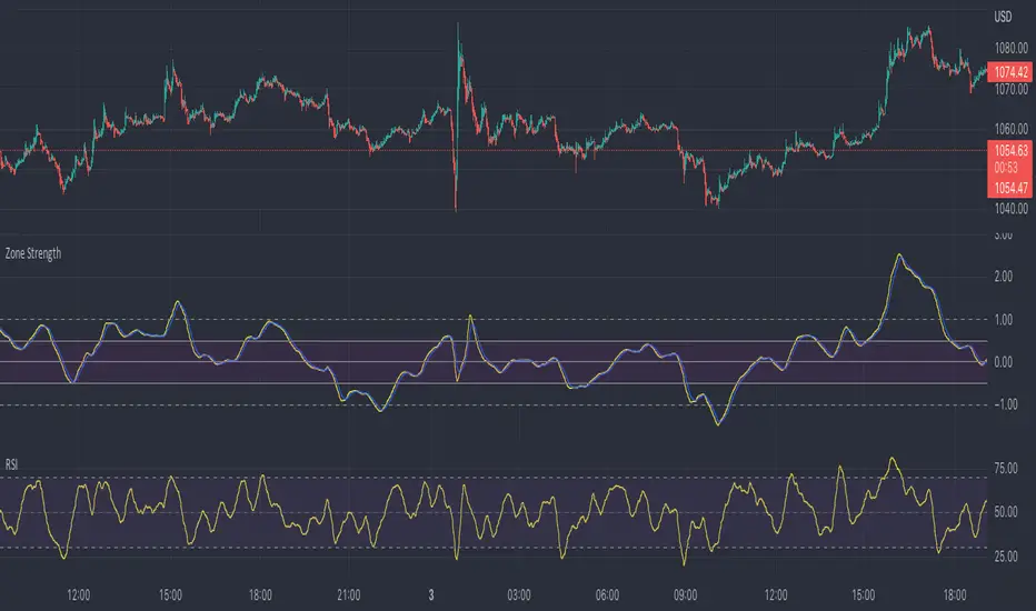
Zone Strength [wbburgin]The Zone Strength indicator is a multifaceted indicator combining volatility-based, momentum-based, and support-based metrics to indicate where a trend reversal is likely.
I recommend using it with the RSI at normal settings to confirm entrances and exits.
The indicator first uses a candle’s wick in relation to its body, depending on whether it closes green or red, to determine ranges of volatility.
The maxima of these volatility statistics are registered across a specific period (the “amplitude”) to determine regions of current support.
The “wavelength” of this statistic is taken to smooth out the Zone Strength’s final statistic.
Finally, the ratio of the difference between the support and the resistance levels is taken in relation to the candle to determine how close the candle is to the “Buy Zone” (<-0.5) or the “Sell Zone” (>0.5).
wbburgin
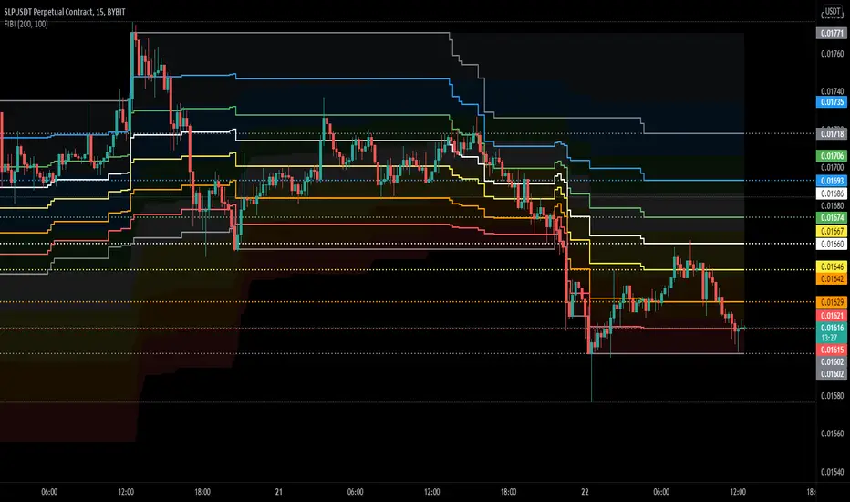
FIBIShows Fibonacci waves for a long range and Fibonacci lines for a short range.
For me it helps to identify key levels or confluence on the macro and micro range.
In the example above you can clearly see that the macro waves are in a down-trend while the micro lines are in a up-trend..
Also the price has been rejected at the 78.6 fib mirco line but found support on the 78.6 macro wave.
these situations are hard to find with the default retracement tools
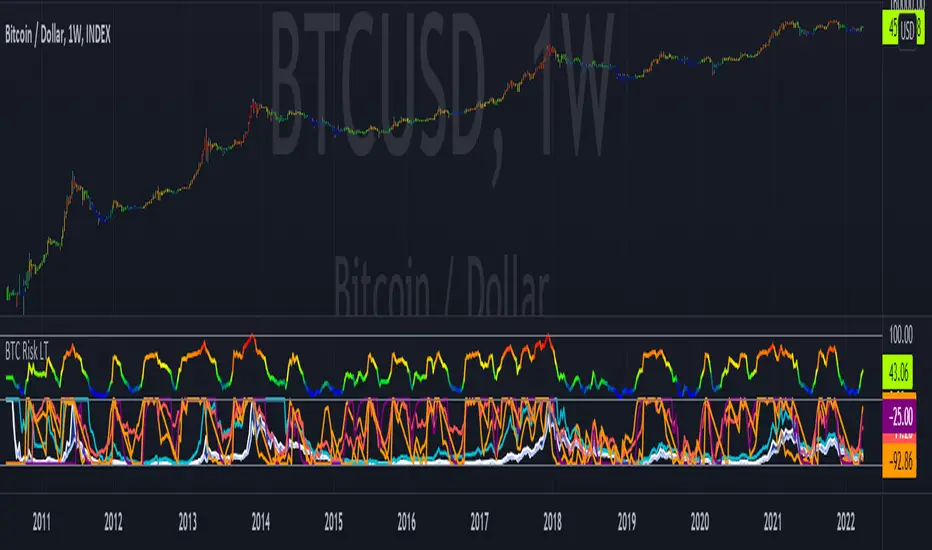
Bitcoin Risk Long Term indicatorOBJECTIVE:
The purpose of this indicator is to synthesize via an average several indicators from a wide choice with in order to simplify the reading of the bitcoin price and that on a long term vision.
Useful for those who want to see things simply, typically to make a smart DCA based on risk.
I originally used this script as a sandbox to understand and test the usefulness of several indicators, and to develop my PineScript skills, but finally the Risk Indicator output seems relevant so I decided to share it.
USAGE:
The selected indicators are the ones that I think give the best market bottoms, but the idea here is that anyone can try and use any set of indicators based on those preferences (post in comments if you find a relevant config)
Most of the indicator inputs are configurable. And some are not taken into account in the calculation of the Risk indicator because I consider them not relevant, this script is also a test more than a final version.
NOTES :
If you have any idea of adding an indicator, modification, criticism, bug found: share them, it is appreciated!
In the future I will create another more versatile Risk indicator that will not be focused on bitcoin in weekly. (this indicator is still usable on other assets and timeframe)
THANKS:
to Benjamin Cowen for inspiring me with his Bitcoin Risk metric
to Lazybear for his Wavetrend Indicator and all the scripts he shares
to Mabonyi for his Bitcoin Logarithmic Growth Curves & Zones script
to VuManChu for his VMC Cypher B Divergence
to the Trading view team for developing TV and PineScript
And to all the community for all the published codes that allowed me to progress and create this script
---- FR ----
OBJECTIF :
L'objectif de cet indicateur est de synthétiser via une moyenne plusieurs indicateurs parmi un large choix avec afin de simplifier la lecture du cours de bitcoin et cela sur une vision longue terme.
Utile pour ceux qui veulent voir les choses simplement, typiquement faire un DCA intelligent en fonction du risque.
À la base j'ai utilisé ce script comme un bac à sable pour comprendre puis tester l'utilité de plusieurs indicateurs, et développer mes compétences PineScript, mais finalement l'output Risk Indicateur me semble pertinent donc autant le partager.
UTILISATION :
Les indicateurs sélectionnés sont ceux qui permettent selon moi d'avoir les meilleurs point bas de marché, mais l'idée ici est que chacun puisse essayer et utiliser n'importe quel ensemble d'indicateur en fonction de ces préférences (poster en commentaire si vous trouvez une configuration pertinente)
La plupart des inputs indicateurs sont paramétrables. Et certains ne sont pas pris en compte dans le calcul du Risk indicateur car je les estime non pertinent, ce script est aussi un essai plus qu'une version finale.
NOTES :
Si vous avez la moindre idée d'ajout d'indicateur, modification, critique, bug trouvé : partagez-les, c'est apprécié !
à l'avenir je créerais un autre Risk indicator plus polyvalent qui ne sera pas focalisé sur bitcoin en weekly. (cet indicateur est tout de même utilisable sur d'autre actif et timeframe)
REMERCIEMENT :
à Benjamin Cowen pour m'avoir inspiré avec son Bitcoin Risk metric
à Lazybear pour son Wavetrend Indicator et globalement tout les scripts qu'il partage
à Mabonyi pour son script Bitcoin Logarithmic Growth Curves & Zones
à VuManChu pour son VMC Cypher B Divergence
à l'équipe Trading view pour avoir développé TV et PineScript
Et à toute la communauté pour tous les codes publiés qui m'ont permis de progresser et de créer ce script
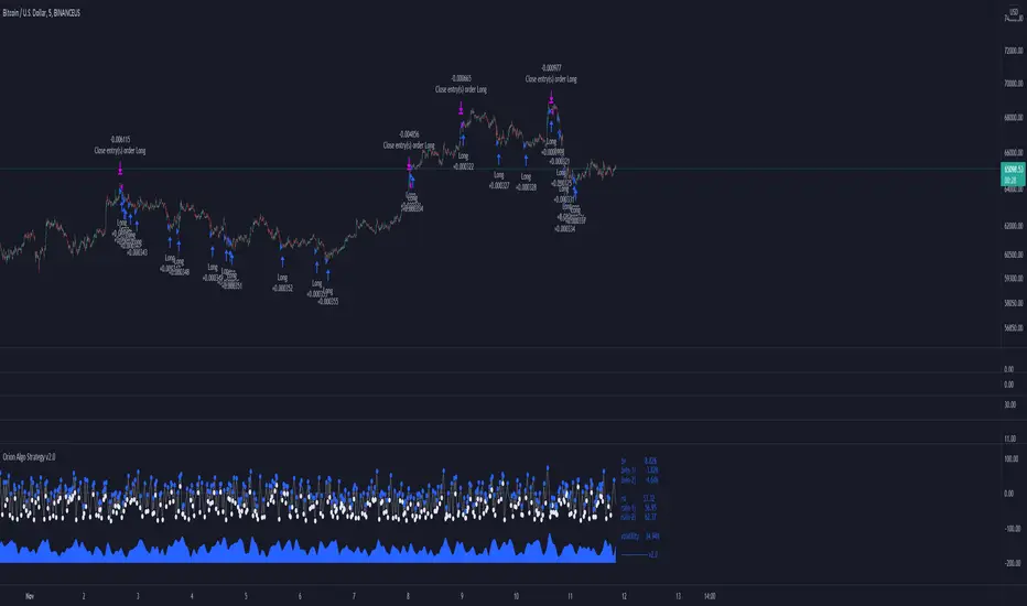
Orion Algo Strategy v2.0Hi everyone.
I decided to make the latest Orion Algo open to people. I don't have enough time to work on it lately, so I figured it would be best that everyone can have it to work on it. I took out some stuff from the original but it should give an idea on how things work. I made two strategies with this so far so you can use that to come up with your own. I recommend the DCA strategy because it gives you the most bang for Orion Algo's buck. It's pretty good at finding long entries.
Overall I hope you guys like this one. Also, Banano is the best crypto currency :)
-INFO-
Orion Algo is a trading algorithm designed to help traders find the highs and lows of the market before, during, and after they happen. We wanted to give an indicator to people that was simple to use. In fact we created the algorithm in such a way that it currently only needs a single input from the user. Since no indicator can predict the market perfectly, Orion should be used as just another tool (although quite a sharp one) for you to trade with. Fundamental knowledge of price action and TA should be used with Orion Algo.
Being an oscillator, Orion currently has a bias towards market volatility . So you will want to be trading markets over 30% volatility . We have plans to develop future versions that take this into account and adjust automatically for dead conditions. Also, while there are some similarities across all oscillators, what sets ours apart is the prediction curve. The prediction curve looks at the current signal values and gives it a relative score to approximate tops and bottoms 1-2 bars ahead of the signal curve. We also designed a velocity curve that attempts to predict the signal curve 2+ bars ahead. You can find the relative change in velocity in the Info panel. The bottom momentum wave is based on the signal curve and helps find overall market direction of higher time-frames while in a lower one.
Settings and How to Use them:
User Agreement – Orion Algo is a tool for you to use while trading. We aren’t responsible for losses OR the gains you make with it. By clicking the checkbox on the left you are agreeing to the terms.
Super Smooth – Smooths the main signal line based on the value inside the box. Lower values shift the pivot points to the left but also make things more noisy. Higher values move things to the right making it lag a bit more while creating a smoother signal. 8 is a good value to start with.
Theme – Changes the color scheme of Orion.
Dashboard – Turns on a dashboard with useful stats, such as Delta v, Volatility , Rsi , etc. Changing the value box will move the dashboard left and right.
Prediction – A secondary prediction model that attempts to predict a reversal before it happens (0-2bars). This can be noisy some times so make your best judgement. Curve will toggle a curve view of the prediction. Pivots will toggle bull/bear dots.
∆v – Delta v (change in velocity). This shows momentum of the signal. Crossing 0 signals a reversal. If you see the delta v changing direction, it may signify a reversal in the several bars depending on the overall momentum of the market.
Momentum Wave – Uses the signal as a macro trend indicator. Changes in direction of the wave can signify macro changes in the market. Average will toggle an averaging algorithm of the momentum waves and makes it easy to understand.
-STRATEGIES-
Simple - Just buy and sell on the dots
DCA - Uses the settings in the script for entries. If a buy dot appears then it will buy, if the price goes below the percentage it will wait for another dot before entering. This drastically improves DCA potential.
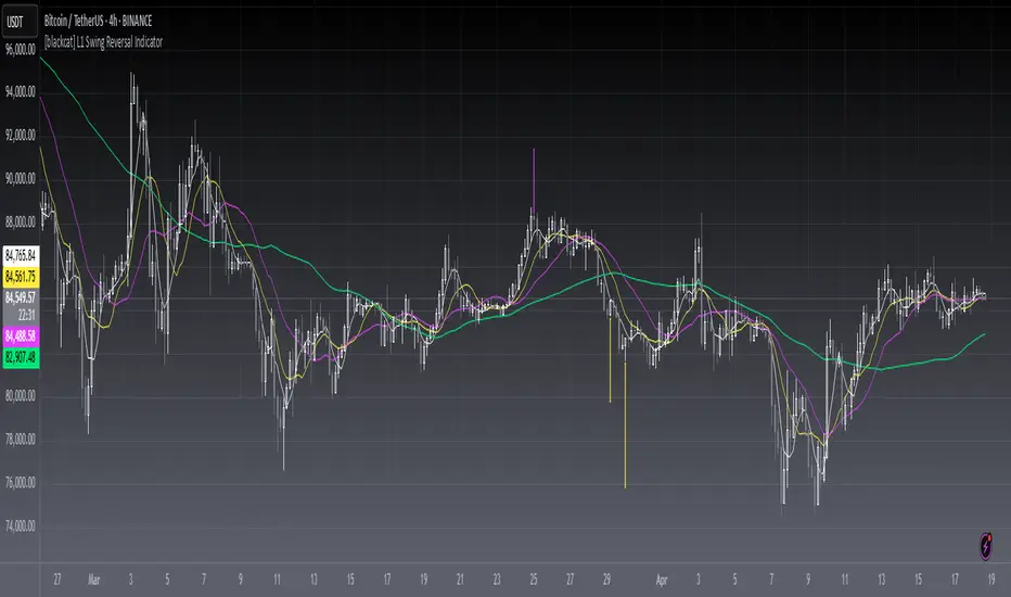
[blackcat] L1 Swing Reversal IndicatorLevel: 1
Background
Many asked me about swing reversal indicators. There are many but less of them can guarantee high win rate. Because market is complex, the reversals can be nested together, which means sub level reversals will be contained in higher level waves. This can be well explained by Elloit wave theory.
Function
Here it is a simple moving average based swing reversal indicator as an example for many others to improve it. Although it simple, it could be very powerful to dedicated trading pairs in specific time frame. One can adjust N1~N4 as SMA peiords from short to long to customized this indicator or even by trying different moving average types to enhance its accuracy.
Key Signal
N1~N4 --> SMA look back periods
OB --> Overbought Threshold
OS --> Oversold Threshold
Pros and Cons
Simpe but powerful. More feedbacks are appreciated.
Remarks
Easy to be customized or integrated to your trading system.
Readme
In real life, I am a prolific inventor. I have successfully applied for more than 60 international and regional patents in the past 12 years. But in the past two years or so, I have tried to transfer my creativity to the development of trading strategies. Tradingview is the ideal platform for me. I am selecting and contributing some of the hundreds of scripts to publish in Tradingview community. Welcome everyone to interact with me to discuss these interesting pine scripts.
The scripts posted are categorized into 5 levels according to my efforts or manhours put into these works.
Level 1 : interesting script snippets or distinctive improvement from classic indicators or strategy. Level 1 scripts can usually appear in more complex indicators as a function module or element.
Level 2 : composite indicator/strategy. By selecting or combining several independent or dependent functions or sub indicators in proper way, the composite script exhibits a resonance phenomenon which can filter out noise or fake trading signal to enhance trading confidence level.
Level 3 : comprehensive indicator/strategy. They are simple trading systems based on my strategies. They are commonly containing several or all of entry signal, close signal, stop loss, take profit, re-entry, risk management, and position sizing techniques. Even some interesting fundamental and mass psychological aspects are incorporated.
Level 4 : script snippets or functions that do not disclose source code. Interesting element that can reveal market laws and work as raw material for indicators and strategies. If you find Level 1~2 scripts are helpful, Level 4 is a private version that took me far more efforts to develop.
Level 5 : indicator/strategy that do not disclose source code. private version of Level 3 script with my accumulated script processing skills or a large number of custom functions. I had a private function library built in past two years. Level 5 scripts use many of them to achieve private trading strategy.
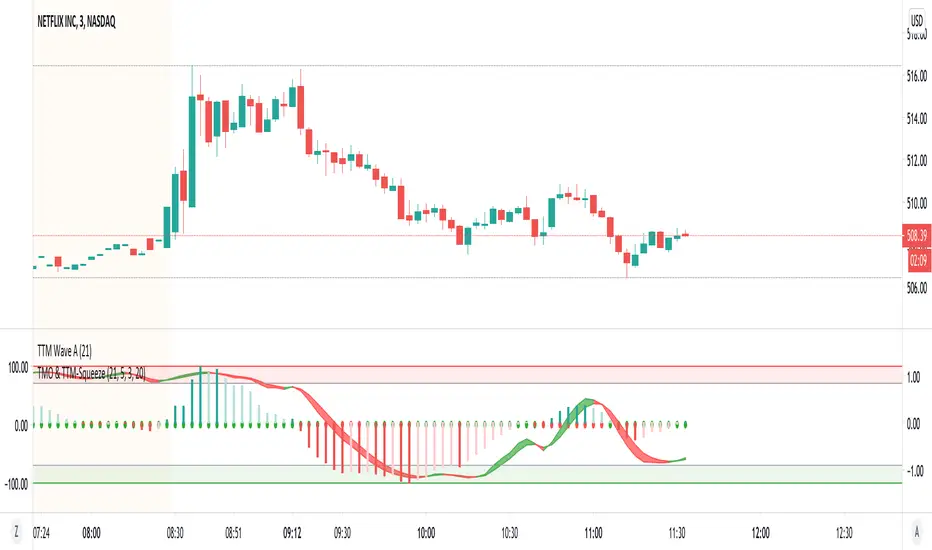
TMO with TTM SqueezeApplication of the TTM squeeze and the short-term momentum TTM Wave A in action. This is an example where the short-term wave will react faster than the TTM to give you a signal to start building your positions.
This indicator needs to be combined with "TTM Wave A" (add to existing pane).
The TTM Squeeze works like a better MACD. There is a zeroline and histogram bars above / below represent positive and negative momo. As the height of the bar decreases when above the zeroline, that is called decreasingly positive momo and as the height of the bar decreases when below the zeroline, that is called decreasingly negative momo. The dots on the TTM Squeeze: Red dots represent consolidation where Bollingers are inside the Keltner Channels and green dots represent a move out of consolidation or "squeeze fire". As price action comes out of consolidation there is a bigger move up/down depending on where momo is heading and where prices are (key support/resistance levels, fib areas). You want to use the TTM Squeeze and A wave TOGETHER - TTM Squeeze is your main momo and your A wave is a short-term momo wave that reacts faster and works as a leading gauge. You need to use them TOGETHER to gauge where price action may be heading. When the TTM Squeeze and A wave move lockstep together, let's say both are decreasingly positive, there is a good probability it continues to move in that direction to the next support levels. TWO bars on the TTM Squeeze of different heights is confirmation that in most cases means it will move in the direction of those bars. So if decreasingly positive, you'll see two darker bars. By the time you get your 2nd bar on the TTM Squeeze, it is often too late or you're losing profit. Way to counter that is after you get one darker bar in the opposite direction of current trend, use A wave to "predict" the next wave, the more A wave histogram bars going towards the other direction, the higher the certainty it will hit. Lastly, using these waves together works best when you look at it on MULTIPLE TIME FRAMES. (Credit for this details goes to Brady from Atlas).
[blackcat] L2 Ehlers Synthetic Prices CandlesLevel: 2
Background
John F. Ehlers create Synthetic Prices Using Random Numbers with Memory in his "Cycle Analytics for Traders" chapter 8 on 2013.
Function
Peter Swerling is best known for the class of statistically “fluctuating target” scattering models he developed in the early 1950s to characterize the performance of pulsed radar systems, referred to as Swerling targets. He noted that the return radar echoes were noisy because of semirandom reflections from different parts of the aircraft because of the changing aspect of aircraft relative to the radar transmitter. There were different kinds of fluctuations due to target shape and size, radar wavelength, and so on. Some fluctuations would occur pulse to pulse, and others would vary more slowly, such as from scan to scan of the antenna. In fact, his early work led to the design of modern stealthy aircraft. The noisy radar echoes were successfully modeled as a constant plus a random number with memory. In terms recognized by traders, the echoes were modeled as an exponential moving average (EMA) passes numbers. The time constant of the EMA was different for the various models, and more complex models included several EMAs. The Swerling model is entirely consistent with the 1/F α spectral model that uses random inputs with long-term memory.
Since there has been a mountain of opinion regarding the randomness of the market, it is reasonable to apply a Swerling-like model toward the generation of synthetic data. The result is subjective, but appears to be a reasonable approximation to real market movement. There is no relationship between the real prices and the synthetic prices. Since random numbers are used, the display will change every time the indicator is computed. Since synthetic prices created by taking an EMA of random numbers are a reasonable approximation to real market prices, the prices can be viewed as random numbers with memory. A logical extension is that we can gain insight into market activity by correlating current prices with prices in the recent history to take advantage of the memory part of the model. At least that was Dr. Ehlers premise.
Key Signal
Cls--> Synthetic Close Prices
Hgh--> Synthetic High Prices
Lw --> Synthetic Low Prices
Opn--> Synthetic Open Prices
Pros and Cons
I am sorry this script is NOT 100% as original Ehlers works but I modified it accordingly which demostrated with better visual effect.
Remarks
The 46th script for Blackcat1402 John F. Ehlers Week publication.
Courtesy of @ midtownsk8rguy for random number generation.
Readme
In real life, I am a prolific inventor. I have successfully applied for more than 60 international and regional patents in the past 12 years. But in the past two years or so, I have tried to transfer my creativity to the development of trading strategies. Tradingview is the ideal platform for me. I am selecting and contributing some of the hundreds of scripts to publish in Tradingview community. Welcome everyone to interact with me to discuss these interesting pine scripts.
The scripts posted are categorized into 5 levels according to my efforts or manhours put into these works.
Level 1 : interesting script snippets or distinctive improvement from classic indicators or strategy. Level 1 scripts can usually appear in more complex indicators as a function module or element.
Level 2 : composite indicator/strategy. By selecting or combining several independent or dependent functions or sub indicators in proper way, the composite script exhibits a resonance phenomenon which can filter out noise or fake trading signal to enhance trading confidence level.
Level 3 : comprehensive indicator/strategy. They are simple trading systems based on my strategies. They are commonly containing several or all of entry signal, close signal, stop loss, take profit, re-entry, risk management, and position sizing techniques. Even some interesting fundamental and mass psychological aspects are incorporated.
Level 4 : script snippets or functions that do not disclose source code. Interesting element that can reveal market laws and work as raw material for indicators and strategies. If you find Level 1~2 scripts are helpful, Level 4 is a private version that took me far more efforts to develop.
Level 5 : indicator/strategy that do not disclose source code. private version of Level 3 script with my accumulated script processing skills or a large number of custom functions. I had a private function library built in past two years. Level 5 scripts use many of them to achieve private trading strategy.

Combo Backtest 123 Reversal & Future Lines of Demarcation This is combo strategies for get a cumulative signal.
First strategy
This System was created from the Book "How I Tripled My Money In The
Futures Market" by Ulf Jensen, Page 183. This is reverse type of strategies.
The strategy buys at market, if close price is higher than the previous close
during 2 days and the meaning of 9-days Stochastic Slow Oscillator is lower than 50.
The strategy sells at market, if close price is lower than the previous close price
during 2 days and the meaning of 9-days Stochastic Fast Oscillator is higher than 50.
Second strategy
An FLD is a line that is plotted on the same scale as the price and is in fact the
price itself displaced to the right (into the future) by (approximately) half the
wavelength of the cycle for which the FLD is plotted. There are three FLD's that can be
plotted for each cycle:
An FLD based on the median price.
An FLD based on the high price.
An FLD based on the low price.
WARNING:
- For purpose educate only
- This script to change bars colors.

Combo Strategy 123 Reversal & Future Lines of Demarcation This is combo strategies for get a cumulative signal.
First strategy
This System was created from the Book "How I Tripled My Money In The
Futures Market" by Ulf Jensen, Page 183. This is reverse type of strategies.
The strategy buys at market, if close price is higher than the previous close
during 2 days and the meaning of 9-days Stochastic Slow Oscillator is lower than 50.
The strategy sells at market, if close price is lower than the previous close price
during 2 days and the meaning of 9-days Stochastic Fast Oscillator is higher than 50.
Second strategy
An FLD is a line that is plotted on the same scale as the price and is in fact the
price itself displaced to the right (into the future) by (approximately) half the
wavelength of the cycle for which the FLD is plotted. There are three FLD's that can be
plotted for each cycle:
An FLD based on the median price.
An FLD based on the high price.
An FLD based on the low price.
WARNING:
- For purpose educate only
- This script to change bars colors.

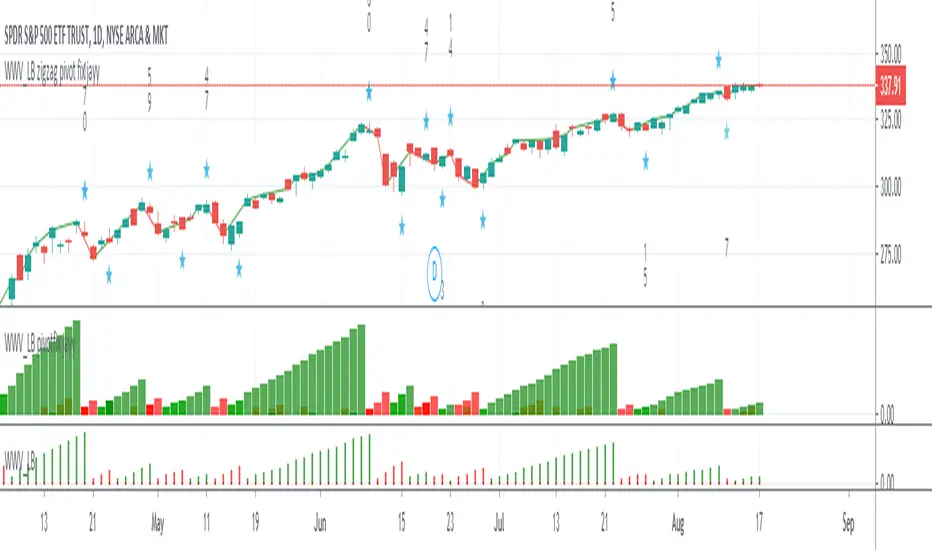
WWV_LB zigzag pivot fix jayyThis is a zigzag version of LazyBear's WWV_LB. In order to plot the WWV_LB as a zigzag, it made sense to me to set the zigzag pivot at the true WWV_LB low or high pivot bars as opposed to the "pivot" bars plotted by the original WWV_LB script. The pivot point identified in the WWV_LB script is actually the point at which a wave reversal is confirmed as opposed to the true script pivot point. Confirmation of a wave reversal can, at times, lag the true pivot by a few bars especially as trendDetectionLength values increase above "1". The WWV_LB script calculates cumulative volume from wave reversal confirmation bar to wave reversal confirmation bar as opposed to the actual/true WWV_LB reversal pivot bar to reversal pivot bar. As such the waves plotted by the original and this pivot fixed scripts not only look slightly different but can also have different cumulative volumes. Confirmation of a wave reversal can lag a few bars behind the true pivot point.
The following critical lines of the original WWV_LB script determine when a wave reverses, both the true pivot and the confirmation point:mov = close>close ? 1 : close
Price Action Trading System v0.3 by JustUncleL with modifcationsThe base of this script is the Price Action Trading System from JustUncle .
I have first combined it with script ADX and DI by BeikabuOyaji to indicate when the +DI is above the -DI and the ADX is above 20. This is represented by crosses at the top of the page: green indicating that the +DI is above the -DI and ADX above 20, and red if -DI is above the +DI and ADX above 20. If the ADX is increasing in slope while the +DI is above the -DI, an up green arrow is shown at the bottom of the page, indicating an increase in this trend, and the slope of the ADX is increasing and the -DI is above the +DI, a down arrow is shown at the bottom. One could think to a green cross with a green up arrow as a potential buy opportunity, and a red cross with a red down arrow as a potential sell opportunity.
Next, I have combined this script with the Indicator: WaveTrend Oscillator from Lazybear . If the oscillator has readings below -45 and the slope of the line is increasing, a green diamond appears above the chart. This indicates a potential buy opportunity. If the oscillator has readings above 50 and the slope of the line is decreasing, a red diamond appears above the chart. This indicates a potential sell opportunity. Now if the slope of the oscillator is rising significantly but does not hit the -45 threshold to start its increase, but is negative in value, a green flag appears at the top of the page. This represents a potential buy opportunity. If the slope of the oscillator is significantly decreasing and is positive in value, a red flag appears at the bottom of the page. This represents a potential sell opportunity.
The base of this script, the Price Action Trading System v0.3 by JustUncle , has many of its own features that I have kept. If the MACD is positive, the background colour is green. If it is negative, the colour is red. If the CCI and RSI indicate an oversold opportunity and the MACD is positive, you get an up olive arrow below the chart. If they indicate an overbought opportunity and the MACD is negative, you get a red down arrow above the chart. If the CCI value stays oversold after a green arrow, the candle chart turns turquoise, and if overbought, turns black after a red arrow.
You can use these indicators in combination to help you with your trading strategy.

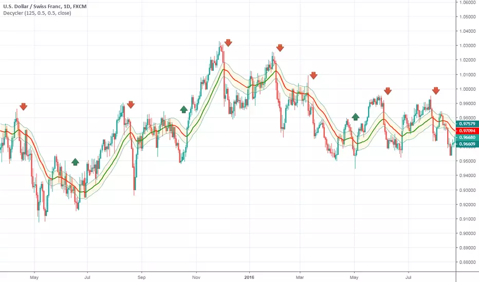
Ehlers Simple DecyclerThis indicator was originally developed by John F. Ehlers (Stocks & Commodities, V.33:10 (September, 2015): "Decyclers").
Mr. Ehlers suggested a way to improve trend identification using high-pass filters. The basic smoothers like SMA, low-pass filters, have considerable lag in their display. Mr. Ehlers applied the high-pass filter and subtracted the high-pass filter output from the time series input. Doing these steps he removed high-frequency short-wavelength components (the ones causing the wiggles) from the time series.
As a result he got a special series of the low-frequency components with virtually no lag - the Decycler.
The Decycler is plotted with two additional lines (the percent-shifts of Decycler) and together they form a hysteresis band.
If the prices are above the upper hysteresis line, then the market is in an uptrend . If the prices are below the low hysteresis line, then the market is in a downtrend . Prices within the hysteresis band are trend-neutral .
Simple TrenderOriginates from:
I was reading some Impulse Trading literature by A. Elder.. In it, someone named Kerry Lovvorn proposed "An End of Day Trend Following System" for someone lazy.
Originally it is just price closing above an 8 ema (low) for long. Exit when price closes below an 8 ema (low). The opposite for a short position.
Conditions: Buy when price closed below ema (low) for two bars or more, then closes above. Opposite for a short position. I do not follow this condition. Though it may help with whipsaw.
My condition is when price closes above the 26 ema (low) (works the best for me) I place orders above the initial crossing bars high. Opposite for lows.
I look for stocks that are low in price to go long on. I want the run from 2's to 15's
I look for stocks that are mid-teens/20's in price to go short on. I want the run from 20's to 2's
I look for stock with news and earnings that are already running (up or down) to play the pullback.
These conditions can easily be scanned for on thinkorswim
From first glance, the system looks like CMsling shotsystem. Although, I plagiarized some parts of the codes, because I am inept when it comes to that shit, it differs as it is not a moving average crossover system.
It is a price crossing over concept. A moving average VWAP is used for best entries on pullbacks.
Purpose:
--To catch the majority of a trend/wave/run.
--To identify pullback areas to go long or short while in midst of trend. To catch pullbacks off news and earning runners.
--To catch the initial start of trend with clear rules to enter
--Clear rules to exit
Issues
--possibilities of getting ninja sliced the fuck up. Can be mitigated by entering stocks with decent average volume. And also only going long above 200 ema and short below it. ADX won't work, at the initial start of the trend it will show not trending. Can look at blow off volume at the bottom followed by increase in buying for long and vice versa for short.
--Can give some huge gains away through gap ups or gap downs from news or earnings during trend. However, can get huge gain on gaps from news or earning. Nature of the game.
--Need some brass balls and a supply of pepto to stomach through some of the pullbacks. Gut wrenching seeing big gains dwindle. But they all even out at the end, you hope. (see NBEV and IGC, and CRON and others. shit don't go in straight lines, homie)
Pros
--It's simple and easy. Overall, you profit
--works with any security
Cons
--It can be stressful.
--does not work well on lower time frames. Do not recommend going below 15 minutes
--Possibility of working on 5 minutes with a time frame breakout strategy (15,30 min).
Couple it with LazyBear "Weis Wave Volume" indicator. Works well for pullback entries.
Enjoy. Ride some waves.

Godmode RSIbased on the popular Godmode Indicator with modifications by LEGION, LAZYBEAR, Ni6HTH4wK, xSilas, oh92, sco77m4r7in
All Credit belongs to them. THX Guys!
This is a Combination of a RSI and Godmode.
RSI has a Simple or Exponential Moving Average, Histogram Color Changes when the RSI reaches the Overbought/Oversold Zones.
Godmode is basicly the same as the Original one only scaled down a bit with slightly adjusted Caution Signal Zones which i like more. I also added the Option to adjust the Length of the 2nd Wavetrend SMA. Removed the Wavetrend Area because it doesnt have any use for me.
Hope you like it.