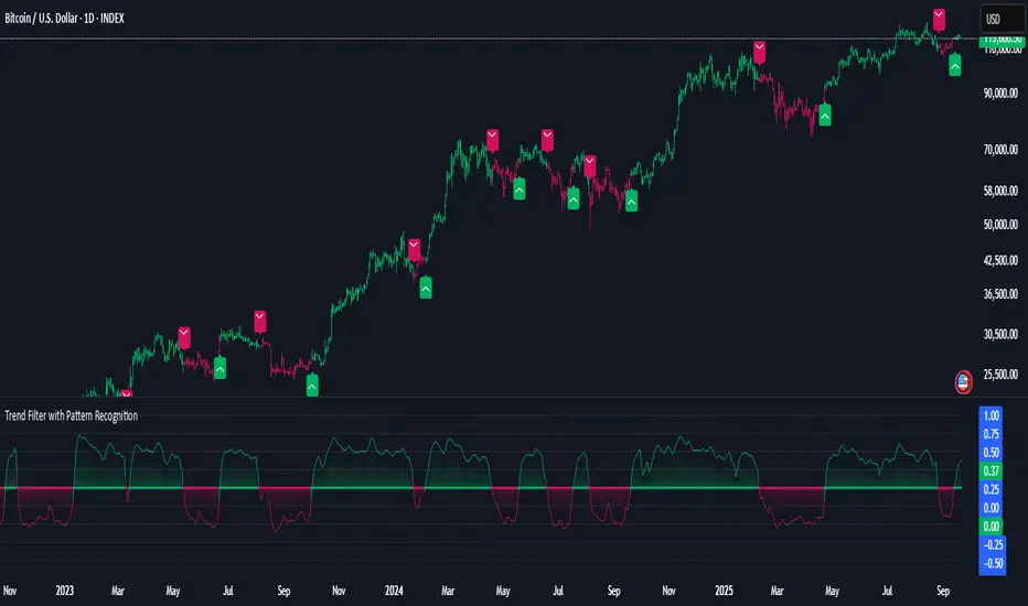
Wavelet-Trend ML Integration [Alpha Extract]Alpha-Extract Volatility Quality Indicator
The Alpha-Extract Volatility Quality (AVQ) Indicator provides traders with deep insights into market volatility by measuring the directional strength of price movements. This sophisticated momentum-based tool helps identify overbought and oversold conditions, offering actionable buy and sell signals based on volatility trends and standard deviation bands.
🔶 CALCULATION
The indicator processes volatility quality data through a series of analytical steps:
Bar Range Calculation: Measures true range (TR) to capture price volatility.
Directional Weighting: Applies directional bias (positive for bullish candles, negative for bearish) to the true range.
VQI Computation: Uses an exponential moving average (EMA) of weighted volatility to derive the Volatility Quality Index (VQI).
Smoothing: Applies an additional EMA to smooth the VQI for clearer signals.
Normalization: Optionally normalizes VQI to a -100/+100 scale based on historical highs and lows.
Standard Deviation Bands: Calculates three upper and lower bands using standard deviation multipliers for volatility thresholds.
Signal Generation: Produces overbought/oversold signals when VQI reaches extreme levels (±200 in normalized mode).
Formula:
Bar Range = True Range (TR)
Weighted Volatility = Bar Range × (Close > Open ? 1 : Close < Open ? -1 : 0)
VQI Raw = EMA(Weighted Volatility, VQI Length)
VQI Smoothed = EMA(VQI Raw, Smoothing Length)
VQI Normalized = ((VQI Smoothed - Lowest VQI) / (Highest VQI - Lowest VQI) - 0.5) × 200
Upper Band N = VQI Smoothed + (StdDev(VQI Smoothed, VQI Length) × Multiplier N)
Lower Band N = VQI Smoothed - (StdDev(VQI Smoothed, VQI Length) × Multiplier N)
🔶 DETAILS
Visual Features:
VQI Plot: Displays VQI as a line or histogram (lime for positive, red for negative).
Standard Deviation Bands: Plots three upper and lower bands (teal for upper, grayscale for lower) to indicate volatility thresholds.
Reference Levels: Horizontal lines at 0 (neutral), +100, and -100 (in normalized mode) for context.
Zone Highlighting: Overbought (⋎ above bars) and oversold (⋏ below bars) signals for extreme VQI levels (±200 in normalized mode).
Candle Coloring: Optional candle overlay colored by VQI direction (lime for positive, red for negative).
Interpretation:
VQI ≥ 200 (Normalized): Overbought condition, strong sell signal.
VQI 100–200: High volatility, potential selling opportunity.
VQI 0–100: Neutral bullish momentum.
VQI 0 to -100: Neutral bearish momentum.
VQI -100 to -200: High volatility, strong bearish momentum.
VQI ≤ -200 (Normalized): Oversold condition, strong buy signal.
🔶 EXAMPLES
Overbought Signal Detection: When VQI exceeds 200 (normalized), the indicator flags potential market tops with a red ⋎ symbol.
Example: During strong uptrends, VQI reaching 200 has historically preceded corrections, allowing traders to secure profits.
Oversold Signal Detection: When VQI falls below -200 (normalized), a lime ⋏ symbol highlights potential buying opportunities.
Example: In bearish markets, VQI dropping below -200 has marked reversal points for profitable long entries.
Volatility Trend Tracking: The VQI plot and bands help traders visualize shifts in market momentum.
Example: A rising VQI crossing above zero with widening bands indicates strengthening bullish momentum, guiding traders to hold or enter long positions.
Dynamic Support/Resistance: Standard deviation bands act as dynamic volatility thresholds during price movements.
Example: Price reversals often occur near the third standard deviation bands, providing reliable entry/exit points during volatile periods.
🔶 SETTINGS
Customization Options:
VQI Length: Adjust the EMA period for VQI calculation (default: 14, range: 1–50).
Smoothing Length: Set the EMA period for smoothing (default: 5, range: 1–50).
Standard Deviation Multipliers: Customize multipliers for bands (defaults: 1.0, 2.0, 3.0).
Normalization: Toggle normalization to -100/+100 scale and adjust lookback period (default: 200, min: 50).
Display Style: Switch between line or histogram plot for VQI.
Candle Overlay: Enable/disable VQI-colored candles (lime for positive, red for negative).
The Alpha-Extract Volatility Quality Indicator empowers traders with a robust tool to navigate market volatility. By combining directional price range analysis with smoothed volatility metrics, it identifies overbought and oversold conditions, offering clear buy and sell signals. The customizable standard deviation bands and optional normalization provide precise context for market conditions, enabling traders to make informed decisions across various market cycles.
Cerca negli script per "wave"
Parsifal.Swing.CompositeThe Parsifal.Swing.Composite indicator is a module within the Parsifal Swing Suite, which includes a set of swing indicators such as:
• Parsifal Swing TrendScore
• Parsifal Swing Composite
• Parsifal Swing RSI
• Parsifal Swing Flow
Each module serves as an indicator facilitating judgment of the current swing state in the underlying market.
________________________________________
Background
Market movements typically follow a time-varying trend channel within which prices oscillate. These oscillations—or swings—within the trend are inherently tradable.
They can be approached:
• One-sidedly, aligning with the trend (generally safer), or
• Two-sidedly, aiming to profit from mean reversions as well.
Note: Mean reversions in strong trends often manifest as sideways consolidations, making one-sided trades more stable.
________________________________________
The Parsifal Swing Suite
The modules aim to provide additional insights into the swing state within a trend and offer various trigger points to assist with entry decisions.
All modules in the suite act as weak oscillators, meaning they fluctuate within a range but are not bounded like true oscillators (e.g., RSI, which is constrained between 0% and 100%).
________________________________________
The Parsifal.Swing.Composite – Specifics
This module consolidates multiple insights into price swing behavior, synthesizing them into an indicator reflecting the current swing state.
It employs layered bagging and smoothing operations based on standard price inputs (OHLC) and classical technical indicators. The module integrates several slightly different sub-modules.
Process overview:
1. Per candle/bin, sub-modules collect directional signals (up/down), with each signal casting a vote.
2. These votes are aggregated via majority counting (bagging) into a single bin vote.
3. Bin votes are then smoothed, typically with short-term EMAs, to create a sub-module vote.
4. These sub-module votes are aggregated and smoothed again to generate the final module vote.
The final vote is a score indicating the module’s assessment of the current swing state. While it fluctuates in a range, it's not a true oscillator, as most inputs are normalized via Z-scores (value divided by standard deviation over a period).
• Historically high or low values correspond to high or low quantiles, suggesting potential overbought or oversold conditions.
• The chart displays a fast (orange) and slow (white) curve against a solid background state.
• Extreme values followed by curve reversals may signal upcoming mean-reversions.
Background Value:
• Value > 0: shaded green → bullish mode
• Value < 0: shaded red → bearish mode
• The absolute value indicates confidence in the mode.
________________________________________
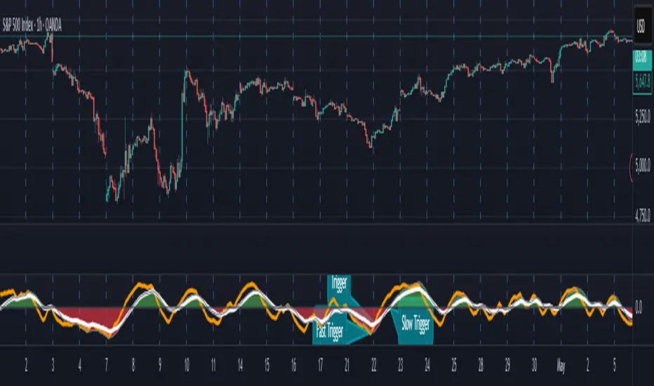
How to Use the Parsifal.Swing.Composite
Several change points in the indicator serve as potential entry triggers:
• Fast Trigger: change in slope of the fast curve
• Trigger: fast line crossing the slow line or change in the slow curve’s slope
• Slow Trigger: change in sign of the background value
These are illustrated in the introductory chart.
Additionally, market highs and lows aligned with swing values may act as pivot points, support, or resistance levels for evolving price processes.
________________________________________
As always, supplement this indicator with other tools and market information. While it provides valuable insights and potential entry points, it does not predict future prices. It reflects recent tendencies and should be used judiciously.
________________________________________
Extensions
All modules in the Parsifal Swing Suite are simple yet adaptable, whether used individually or in combination.
Customization options:
• Weights in EMAs for smoothing are adjustable
• Bin vote aggregation (currently via sum-of-experts) can be modified
• Alternative weighting schemes can be tested
Advanced options:
• Bagging weights may be historical, informational, or relevance-based
• Selection algorithms (e.g., ID3, C4.5, CAT) could replace the current bagging approach
• EMAs may be generalized into expectations relative to relevance-based probability
• Negative weights (akin to wavelet transforms) can be incorporated
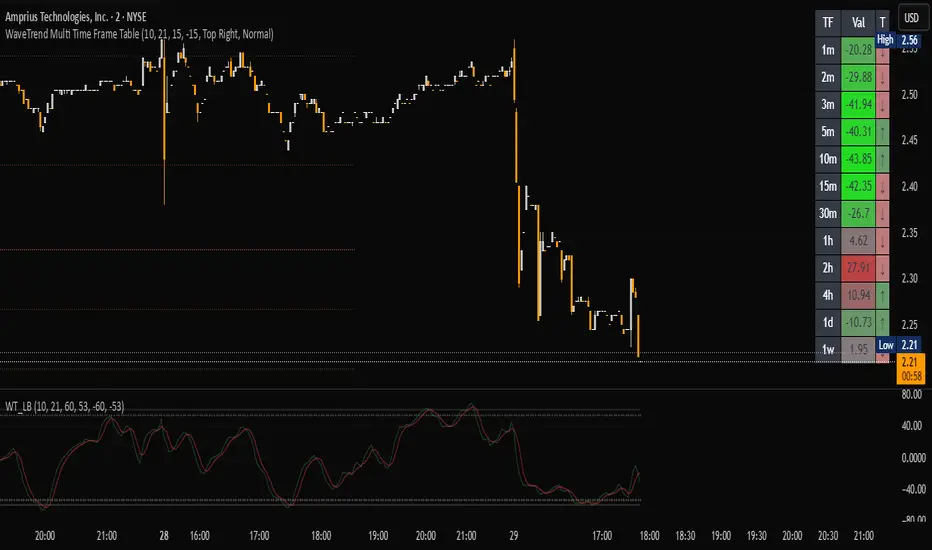
WaveTrend Matrix (1m-1w) – Custom ThresholdsA visual control panel for momentum exhaustion across ten key time-frames.
—
🧬 DNA
This is a fork of LazyBear’s original WaveTrend Oscillator .
The oscillator logic is 100 % intact; I simply stream the values into a compact table so that day- and swing-traders can see the “bigger picture” at a glance.
📈 What does it do?
Calculates WaveTrend on ten granularities: 1m, 3m, 5m, 15m, 30m, 1h, 2h, 4h, 1d, 1w.
Displays the current oscillator print in a color-coded matrix.
• Red = overbought (≥ high threshold)
• Green = oversold (≤ low threshold)
• Gray = neutral / in-range
All thresholds are user-adjustable.
Built on Pine v5, zero repainting, works on any symbol.
🛠 Parameters
Channel Length – WT “n1” (default 10)
Average Length – WT “n2” (default 21)
Red from – overbought cut-off (default +60)
Green under – oversold cut-off (default –60)
🚀 How to use it
1. Apply the indicator to your chart – no extra setup required.
2. Read the matrix top-down before every entry:
• Multiple deep-green rows → market broadly oversold → watch for longs.
• Multiple deep-red rows → market broadly overbought → watch for shorts or stay flat.
3. Combine with your trend filter (EMA-stack, VWAP, structure) to avoid counter-trend trades.
Market Structures + ZigZag [TradingFinder] CHoCH/BOS - MSS/MSB🟣 Introduction
🔵 Market Structure
Grasping market structure entails examining market behavior. Essentially, market structure refers to the formation and progression of the market within its trends.
Market structures are generally fractal and nested, leading us to classify them into internal (minor) and external (major) structures. There are several definitions of market structure, with differing perspectives such as Smart Money and ICT offering their own interpretations.
🔵 Zig Zag
The Zigzag indicator is a lagging tool that identifies points on a price chart where significant changes occur compared to the previous wave. By connecting these points, it helps traders detect trends.
This indicator minimizes random price fluctuations, aiming to clarify the primary price trend.
Pivots are points on a price chart where the direction changes. Also known as reversal points, pivots form when supply and demand forces overpower one another.
There are various types of technical analysis pivots, which can be divided into two categories: minor pivots and major pivots, each with distinct significance in analysis.
Major Pivot : These pivots signify substantial changes in the chart's direction and occur at the end of trends. Analysts focusing on primary analysis prioritize major pivot points. In fact, most technical analysis tools are evaluated and based on major pivots.
Minor Pivot : These pivots highlight smaller, subsidiary points and directions, appearing at the end of corrections. Analysts who focus on minor pivots represent small trends. It's important to note that minor pivots are not suitable for use in primary technical tools.
Identifying Minor and Major Pivots :
Minor pivots are formed between two major pivots and do not break the opposing major pivot. (Internal Pivot)
Major pivots are those that either successfully break the opposing pivot or move beyond the previous pivot of the same type. (External Pivot)
🟣 How to Use
🔵 Identifying Break of Structure (BOS)
In a given trend, such as a downtrend, a Break of Structure occurs when the price drops below the previous low and forms a new low (LL). In an uptrend, a BOS (MSB) happens when the price rises and exceeds the last high.
To confirm a trend, at least one BOS is required. The break above or below the previous high or low must be validated by the closing of at least one candle beyond that level.
🔵 Identifying Change of Character (CHOCH)
Change of Character (CHOCH) is an essential concept in market structure analysis, indicating a trend change. In other words, a trend concludes with a CHOCH (MSS). For example, in a downtrend, the price declines with BOS.
While BOS highlights the trend's strength, a CHOCH occurs when the price rises and surpasses the last high, signaling a transition from a downtrend to an uptrend.
This does not imply immediately entering a buy trade; instead, it is prudent to wait for a BOS in the upward direction to confirm the uptrend.
Unlike BOS, confirming a CHOCH does not require a candle to close; simply breaking above or below the previous high or low with the candle's wick is sufficient. The following examples illustrate bearish and bullish CHOCH.
Terms :
Market Structure Shift = MSS
Market Structure Break = MSB
🔵 Zig Zag
Based on identifying pivots and drawing zigzag lines, you can have different uses of this indicator.
Including :
Identifying pivot types along with major and minor recognition.
Identifying internal and external breakouts.
Identifying support and resistance levels.
Identifying Elliott Waves.
Identifying classic patterns.
Identifying pivots with higher validity.
Identifying trends and range areas.
🟣 Settings
Pivot Period Market Structure and ZigZag Line: Using this input, you can determine the pivot period for identifying swings.
Through the settings, you can customize the display, visibility, and color of each line as desired.

WaveTrendnel Oscillator [UAlgo]🔶Description:
The WaveTrendnel Oscillator, is a technical analysis tool designed for traders to identify potential trend reversals and overbought/oversold conditions in the market. It combines the concepts of wave analysis and trend analysis to generate signals based on the current market conditions. This indicator aims to provide traders with insights into the strength and direction of the prevailing trend, facilitating better decision-making in trading strategies.
🔶Key Features:
Customizable Parameters: Users can customize various parameters including the source data, channel length, average length, and signal length according to their trading preferences and market conditions.
Signal Display: The indicator offers the option to display buy and sell signals on the chart, helping traders to visually identify potential entry and exit points.
Wave and Kernel Analysis: The WaveTrendnel Oscillator utilizes a rational quadratic kernel function, which applies a mathematical approach known as the kernel method. This method analyzes historical price data by assigning weights to each data point based on its proximity to the current period, providing a smoother and more accurate representation of market trends.
Overbought/Oversold Levels: Traders can define overbought and oversold levels using customizable threshold parameters, enabling them to identify potential reversal points in the market.
🔶Credit:
The WaveTrendnel Oscillator indicator is a modification of the original WaveTrend Oscillator developed by @LazyBear on TradingView.
🔶Disclaimer:
Use with Caution: This indicator is provided for educational and informational purposes only and should not be considered as financial advice. Users should exercise caution and perform their own analysis before making trading decisions based on the indicator's signals.
Not Financial Advice: The information provided by this indicator does not constitute financial advice, and the creator (UAlgo) shall not be held responsible for any trading losses incurred as a result of using this indicator.
Backtesting Recommended: Traders are encouraged to backtest the indicator thoroughly on historical data before using it in live trading to assess its performance and suitability for their trading strategies.
Risk Management: Trading involves inherent risks, and users should implement proper risk management strategies, including but not limited to stop-loss orders and position sizing, to mitigate potential losses.
No Guarantees: The accuracy and reliability of the indicator's signals cannot be guaranteed, as they are based on historical price data and past performance may not be indicative of future results.

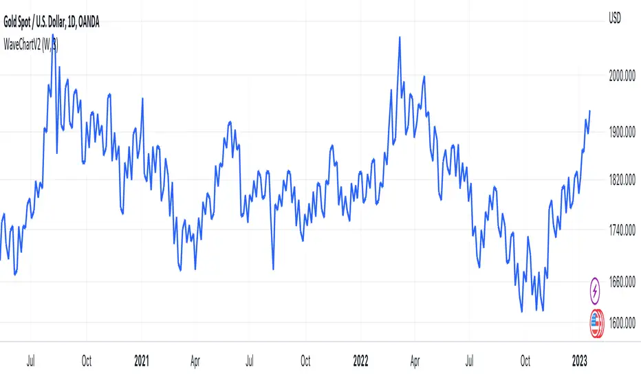
Wavechart v2 ##Wave Chart v2##
For analyzing Neo-wave theory
Plot the market's highs and lows in real-time order.
Then connect the highs and lows
with a diagonal line. Next, the last plot of one day (or bar) is connected with a straight line to the
first plot of the next day (or bar).
.236 FIB Extension ToolThis is a simple FIB extension tool that pulls from the start of a wave to the end of the wave. It extends FIB levels beyond the first wave making the assumption that the first wave was between 0.0 and .236 FIB levels. This often works as support and resistance in a multi-wave move. I see the price get to .65 or .786 often after clearing the initial .236 level. This works on any timeframe.

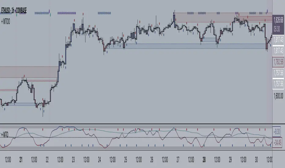
+ WaveTrend Oscillator OverlayAn overlay version of pertinent signals from my version of LazyBear's Wavetrend Oscillator.
Shows momentum of long period WTO as either background colors or symbols.
Shows continuation and reversal trade signals.
If Secondary WTO is above the center line (momentum is long), then symbols print across the top of the chart when the primary (faster) WTO comes into "oversold," a number associated with a horizontal line on the off-chart indicator. This number is selectable via a drop-down menu. Same thing for bearish momentum.
Conversely, reversal signals are printed along the bottom when conditions are met. Ex: if the Secondary WTO is showing momentum is bullish, then symbols will print along the bottom when the primary WTO is at "overbought" (or whatever number you deem overbought--again, via a similar drop-down menu).
Also, symbols are printed above and below candles for when the moving average of the primary WTO is crossed.
You could use these for taking profits, exiting a trade, or entering a trade.
Includes a moving average that is an average of the 200 EMA, SMA and Kijun.
Alerts.
Enjoy.
//p.s. I recommend using this in conjunction with my "+ Wavetrend Oscillator" at least starting out. Helps to have a visual
//reference when picking reversal and continuation numbers.
+ WaveTrend OscillatorI'm guessing most of you are familir with LazyBear's adaptation of the Wavetrend Oscillator; it's one of the most popular indicators on TradingView. I know others have done adaptations of it, but I thought I might as well, because that's kind of a thing I like doing.
In this version I've added a second Wavetrend plot. This is a thing I like to do. The longer plot gives you a longer timeframe momentum bias, and the shorter plot gives you entries and/or exits. Here we have one plot with a lookback period of 55, and another with the default set to 6 (change this to 14 if you think you might prefer something slower and that will plot similarly to the default RSI settings). With the traditional Wavetrend Oscillator there is a simple moving average on the WTO that is to help provide entries and exits. I've done away with this as there are already two plots, and I felt more would just clutter the indicator. Instead of plotting the SMA I've plotted the crosses along the bottom and top of the indicator. Also, as is not the case in LazyBear's version, this SMA length is adjustable. By default it is set to 3, which is the default setting on the original indicator.
I've also plotted background colors for when there is what I call a momentum shift. If one or the other oscillators crosses the centerline a colored bar is plotted. By default it is turned on for both WTOs, though in practice you might only want it on for the longer one.
I would say use of the indicator is similar to the original WTO or many other oscillators. Buying oversold and selling overbought, but being mindful of the momentum of the market. If the longer WTO is above the centerline it's best to be looking for dips to the centerline, or for an overbought signal by the faster WTO, and vice versa if the longer WTO is below the centerline. That said, you can also adjust the length of the SMA on the faster WTO to fine tune entries or exits, which is kind of how you would trade LazyBear's version. In this case you have that additional confirmation of market momentum.
You can set colored candles to either of the WTO plots via a dropdown menu.
There are alerts for overbought and oversold situations, centerline crosses, and Wavetrend crosses.
That's about it. Hope you enjoy this particular implementation of LazyBear's well known indicator.
Ah yes, last thing: Original version the source is set to hlc3. I've given you the opportunity to change that, so if you prefer using close you can, or whatever you want.

Wavetrend strategy with trading session for any time chartHello there
Today I am glad to provide you a strategy based on the wave trend oscillator. If you want to use it as an indicator, just disable long and short to not make any shops.
It works on all time frames.
The way it works its like an RSI .
We have overbought and oversold levels, and together with a channel and length we calculate the wave trend.
And then like in RSI, when we cross those lines we buy or sell depending on which lines we cross.
For risk management, so far its not implemented, but it can be done in many ways.
The only thing I applied is to always close a trade at the end of friday day. At the same time it can be applied the rule to sell when % of equity is lost, or at the end of a trading session like london,neywork and so on.
For any questions or doubts, let me know.
Hope you enjoy it :)

Stochastic Heat MapA series of 28 stochastic oscillators plotted horizontally and stacked vertically from bottom to top as the oscillator background.
Each oscillator has been interpreted and the value has been used to colour the lines in.
Lower lines are shorter term stochastics and higher lines are longer term stochastics.
The average of the 28 stochastics has been taken and then used to plot the fast oscillator line, which also has a slow oscillator line to follow.
The oscillator line can be used to colour in the candles.
Inputs:
MA: multiple smoothing methods
Theme: multiple colours
Increment: stochastic length start and increments
Smooth Fast: smooth fast length
Smooth Slow: smooth slow length
Paint Bars: colour candles
Waves: toggle method to weight/increment stochastics
Heat map shows momentum extremes:

WaveTrend By LimaIndicator packing both WaveTrend and RSI.
Source code for the WaveTrend belongs to LazyBear and RSI well, it is a Pinescript method.

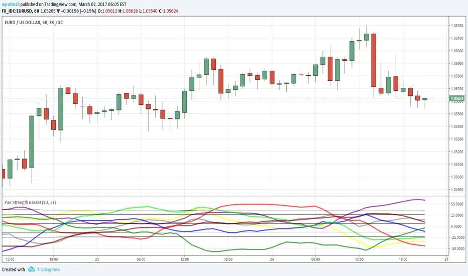
Pair Strength BasketAgain thanks to LazyBear for bringing over the wavetrend indicator and glaz for the idea of the basket of currencies. This is a power index based on the wavetrend indicator, I cut it down to 5 securities per currency since the limit of securities I could call was 40. I like to use to see which pair is the most OB/OS as it likely presents the best profit potential.
AUD = Yellow
CAD = Gray
CHF = Maroon
EUR = Blue
GBP = Red
JPY = Purple
NZD = Lime
USD = Green
STEEMSBD WaveTrendWaveTrend-Oscillator over synthetic STEEM/SBD based on STEEM/BTC and SBD/STB from Poloniex.
WaveTrend part is based on LazyBear's port of TS/MT indicator.

WaveTrend with Crosses [LazyBear]LazyBear's wavetrend oscillator enhanced with wavetrend cross visualization on the indicator as well as with bar color highlights.

Wave Smoother [WS]The Wave Smoother is a unique FIR filter built from the interaction of two trigonometric waves. A cosine carrier wave is modulated by a sine wave at half the carrier's period, creating smooth transitions and controlled undershoot. The Phase parameter (0° to 119°) adjusts the modulating wave's phase, affecting both response time and undershoot characteristics. At 30° phase the impulse response starts at 0.5 and exhibits gentle undershoot, providing balanced smoothing. Higher phase values reduce ramp-up time and increase undershoot - this undershoot in the impulse response creates overshooting behavior in the filter's output, which helps reduce lag and speed up the response. The default 70° phase setting provides maximum speed while maintaining stability, though practical settings can range from 30° to 70°. The filter's impulse response consists entirely of smooth curves, ensuring consistent behavior across all settings. This design offers traders flexible control over the smoothing-speed trade-off while maintaining reliable signal generation.

Wave Generator Library (WGL)Library "WaveGenerator"
Wave Generator Library
max(source)
max
Parameters:
source : is the input to take the maximum.
Returns: foat
min(source)
min
Parameters:
source : is the input to take the minimum.
Returns: foat
min_max(src, height)
min_max
Parameters:
src : is the input for the min/max
height
Returns: float
sine_wave(_wave_height, _wave_duration, _phase_shift, _phase_shift_2)
sine_wave
Parameters:
_wave_height : Maximum output level
_wave_duration : Wave length
_phase_shift : Number of harmonics
_phase_shift_2
Returns: float
triangle_wave(_wave_height, _wave_duration, _num_harmonics, _phase_shift)
triangle_wave
Parameters:
_wave_height : Maximum output level
_wave_duration : Wave length
_num_harmonics : Number of harmonics
_phase_shift : Phase shift
Returns: float
saw_wave(_wave_height, _wave_duration, _num_harmonics, _phase_shift)
saw_wave
Parameters:
_wave_height : Maximum output level
_wave_duration : Wave length
_num_harmonics : Number of harmonics
_phase_shift : Phase shift
Returns: float
ramp_saw_wave(_wave_height, _wave_duration, _num_harmonics, _phase_shift)
ramp_saw_wave
Parameters:
_wave_height : Maximum output level
_wave_duration : Wave length
_num_harmonics : Number of harmonics
_phase_shift : Phase shift
Returns: float
square_wave(_wave_height, _wave_duration, _num_harmonics, _phase_shift)
square_wave
Parameters:
_wave_height : Maximum output level
_wave_duration : Wave length
_num_harmonics : Number of harmonics
_phase_shift : Phase shift
Returns: float
wave_select(style, _wave_height, _wave_duration, _num_harmonics, _phase_shift)
wave_select
@peram style Select the style of wave. "Sine", "Triangle", "Saw", "Ramp Saw", "Square"
Parameters:
style
_wave_height : Maximum output level
_wave_duration : Wave length
_num_harmonics : Number of harmonics
_phase_shift : Phase shift
Returns: float
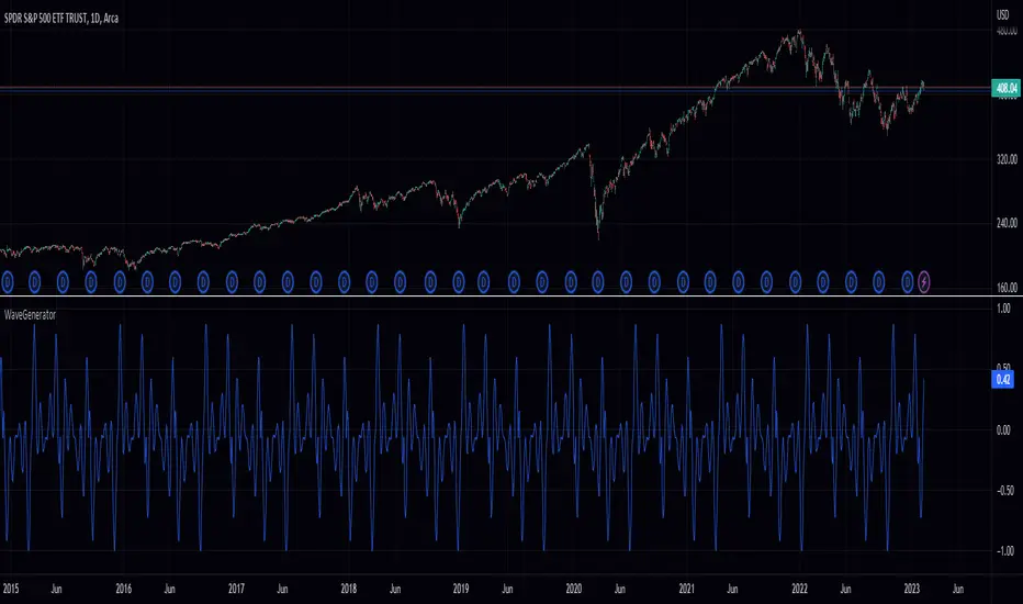
Wave Generator (WG)Pine Script Wave Generator Utility
Introduction:
The Pine Script Wave Generator Utility is a versatile tool that creates different wave patterns. The script provides the user with four different wave styles to choose from (Sine, Triangle, Saw, Square) with customizable parameters for the wave height, duration, number of harmonics, and phase shift.
Technical Details:
The script utilizes the mathematical functions sin, pi, and array.avg to generate wave patterns. The wave height and duration are the main inputs, and the number of harmonics and phase shift are additional inputs that add fine-tuning to the wave pattern.
The wave styles are created using different combinations of sine waves and are normalized so that the resulting wave always lies within a range of -1 to 1.
Usage:
The user can adjust the wave parameters using the input options in the script. The user can choose the wave style from the “Wave Select” option and set the wave height, wave duration, number of harmonics and phase shift by adjusting the corresponding input options.
Conclusion:
The Pine Script Wave Generator Utility is an efficient and effective tool for generating wave patterns. It can be used for a variety of purposes such as creating wave patterns for technical analysis, simulation, and testing purposes. The user can easily adjust the wave parameters to create custom wave patterns, making it a flexible and valuable tool.

WaveTrend & Supertrend Comparison/CombinedThis compares two reasonably reliable strategies and shows where they are in agreement.
When the top line is GREEN - Then consider BUYing
When the top line is RED - Then consider SELLing
There are also alerts available.
WaveTrend with Crosses [LazyBear]Optical Change
Source from LazyBear
With big Hugs for this Indicator

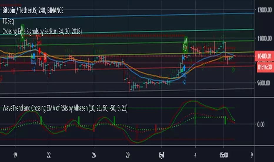
WaveTrend and Crossing EMA of RSIs by AlhazenLazyBear's WaveTrend Oscilator is simplified, and buy & sell signals are added. Green bars indicate SELL signal of WT, and Maroon bars indicate BUY signal of WT.
A new indicator added: Crossing EMA of two RSI's. RSI plots are shown with dotted lines. Lime bars indicate SELL signal of RSI, and Red bars indicate BUY signal of RSI.
You can combine WT and RSI together and decide to BUY or SELL.
WaveTrend mtfThis is based on Lazy Bear famous script of Wave trend
So in basic we do MTF on it
One can choose to use the signal of the MTF (circles red or green for buy and sell)
or the regular buy and sell by cross green /red
to the script one can add if it cross the 0 above or bellow (not done here)
the MTF is taken from pinescripter example how to avoid repainting , so it good also for using your indicator to make MTF scripts
alerts included

