@Complete Squeeze Cycle Detector v2.0 FINALDescription:
The Complete Squeeze Cycle Detector identifies and tracks the full lifecycle of squeeze formations, from pre-squeeze consolidation through active squeeze periods to squeeze completion. The indicator systematically detects the characteristic conditions that precede and accompany squeeze events.
The indicator monitors multiple factors associated with squeeze development including:
• Volatility compression relative to recent volume activity
• Elevated market stress conditions as measured by VIX levels
• Momentum compression through rate of change measurements across multiple time periods
• Alignment of multiple exponential moving averages indicating consolidation
The squeeze cycle is classified into three distinct phases: Pre-Squeeze Setup, Active Squeeze, and Squeeze Complete. Each phase is identified based on threshold levels of multiple compression metrics, with adjustable sensitivity settings to control the strictness of detection.
The indicator provides visual identification of each phase through labels, background coloring, and an optional dashboard, allowing users to distinguish between the preparation phase where volatility contracts, the active squeeze phase where compression reaches critical levels, and the completion phase where the squeeze releases and directional movement resumes.
This systematic approach enables users to identify squeeze formations throughout their complete development cycle rather than focusing only on the breakout phase.
Cerca negli script per "同花顺软件+美国+VIX+恐慌指数+行情代码"

Elite Correlation Matrix AIThe Elite Correlation Matrix AI indicator provides comprehensive real-time correlation analysis across multiple asset classes, displaying the interrelationships between equities, bonds, commodities, currencies, and volatility instruments.
The indicator calculates and displays correlation coefficients between a predefined set of major market indices and instruments, including:
• Major equity indices (SPY, QQQ, IWM)
• Long-term Treasury bonds (TLT)
• Gold (GLD)
• Crude oil (USO)
• Volatility (VIX)
• US Dollar Index (DXY)
• Bitcoin (BTCUSD)
Key features include:
• Rolling correlation calculations across user-defined periods to identify both short-term and longer-term relationships
• Visual correlation heat map showing the strength and direction of relationships between all tracked instruments
• Detection of correlation breakdowns, which often precede significant market regime shifts
• Dashboard display providing summary metrics of prevailing correlation patterns
The indicator enables users to monitor the current state of market relationships and identify when traditional correlations begin to break down, which frequently serves as an early warning of impending changes in market behavior. By tracking the degree of connectedness between different asset classes, the indicator provides insight into the current risk environment and the potential for diversification effectiveness.
This analysis is particularly valuable for understanding periods of market stress when asset relationships deviate from their normal patterns, as well as identifying environments where traditional correlations hold and where they are undergoing structural changes.

Risk On/Risk Off by Gary# Risk On/Risk Off Indicator (RORO)
## Overview
The Risk On/Risk Off (RORO) Indicator is a comprehensive market sentiment gauge that measures the balance between risk-seeking and risk-averse behavior across multiple asset classes. This indicator helps traders identify shifts in market sentiment and potential trend changes.
## How It Works
The RORO indicator aggregates normalized price movements (Z-scores) from eight major asset classes:
**Risk-On Assets (Bullish Sentiment):**
- Bitcoin Futures (BTC1!) - Cryptocurrency risk appetite
- WTI Crude Oil Futures (CL1!) - Energy sector strength
- AUD/JPY Exchange Rate - Carry trade indicator
- Emerging Markets ETF (EEM) - Global growth proxy
**Risk-Off Assets (Defensive Sentiment):**
- Gold Futures (GC1!) - Safe haven demand
- 10-Year Treasury Bonds (ZN1!) - Flight to quality
- US Dollar Index (DXY) - Reserve currency strength
- VIX Index - Market fear gauge (inverted)
## Key Features
- **Z-Score Normalization**: Standardizes different asset classes for fair comparison
- **Customizable Weights**: Adjust the influence of each asset class
- **Dynamic Coloring**: Green indicates rising risk appetite, red shows declining risk appetite
## Interpretation
- **Rising RORO (Green)**: Increasing risk appetite - favorable for equities, commodities, and growth assets
- **Falling RORO (Red)**: Decreasing risk appetite - rotation into safe havens
- **Divergences**: When RORO and price move in opposite directions, potential reversal signal
## Use Cases
1. **Market Regime Identification**: Determine current risk environment
2. **Divergence Trading**: Spot when price action contradicts underlying sentiment
3. **Portfolio Management**: Time defensive vs. aggressive positioning
4. **Confirmation Tool**: Validate breakouts and trend changes
## Settings
- **Lookback Period**: Controls Z-score calculation sensitivity (default: 50)
- **Asset Weights**: Fine-tune the contribution of each asset class
- **Color Scheme**: Customize rising/falling colors
## Best Practices
- Use on daily or higher timeframes for most reliable signals
- Combine with price action and volume analysis
- Watch for sustained moves rather than single-bar changes
---
*This indicator is designed for educational purposes. Always conduct your own analysis and risk management.*

Global Liquidity Score
Global Liquidity Score – Simple Risk-On / Risk-Off Gauge
This indicator measures overall market liquidity conditions using a single, normalized score.
It takes several macro and crypto variables, standardizes each one (z-score), and combines them into one clear Liquidity Score Line.
You only follow one line (your pink/white line).
The background color shows the current liquidity regime.
⸻
What the indicator measures
The algorithm looks at four major liquidity sources:
1. USD Liquidity (tightening or easing)
• DXY (strong dollar = tighter global liquidity)
• US10Y yield (higher yields = liquidity drain)
2. Risk Sentiment (risk-on vs risk-off)
• VIX index (volatility)
• S&P 500 index (SPX)
3. Credit Market Strength
• High-yield ETFs: HYG, JNK
• Investment-grade corporate credit: LQD
Stronger credit = easier liquidity.
Weaker credit = tightening risk.
4. Internal Crypto Liquidity
• USDT dominance (higher = risk-off in crypto)
• Bitcoin price
• TOTAL2 (crypto market cap excluding BTC)
These are all converted into z-scores and combined into one metric:
Total Liquidity Score =
USD Block + Risk Block − Credit Block − 0.5 × Crypto Block
⸻
How to read the colors
The indicator uses background colors to show the liquidity regime:
Color Meaning
Dark Red Severe liquidity tightening / strong risk-off
Red Mild-to-moderate tightening
Green Liquidity easing / soft risk-on
Dark Green Strong easing, high liquidity / risk-on
Your pink/white line = the final liquidity score.
You only need to follow that single line.
⸻
How to interpret the score
📉 Positive score → Liquidity Tightening (Risk-Off)
• USD stronger
• Yields rising
• Volatility rising
• Credit markets weakening
• Crypto rotating to stablecoins
📈 Negative score → Liquidity Easing (Risk-On)
• USD weakening
• Yields falling
• Stocks rising
• Volatility low
• Credit markets strong
• Crypto beta assets outperform
⸻
What this indicator is NOT
This is not a price predictor.
It does not follow BTC directly.
It tells you liquidity conditions, not immediate price direction.
It answers the macro question:
“Is liquidity flowing INTO the market or OUT of the market?”
If liquidity is tightening (red), crypto rallies are harder to sustain.
If liquidity is easing (green), crypto rallies have more fuel.

CNN Fear and Greed StrategyAdaptation of the CNN Fear and Greed Index Indicator (Original by EdgeTools)
The following changes have been implemented:
Put/Call Ratio Data Source: The data source for the Put/Call Ratio has been updated.
Bond Data Source: The data sources for the bond components (Safe Haven Demand and Junk Bond Demand) have been updated.
Normalization Adjustment: The normalization method has been adjusted to allow the CNN Fear and Greed Index to display over a longer historical period, optimizing it for backtesting purposes.
Style Modification: The display style has been modified for a simpler and cleaner appearance.
Strategy Logic Addition: Added a new strategy entry condition: index >= 25 AND index crosses over its 5-period Simple Moving Average (SMA), and a corresponding exit condition of holding the position for 252 bars (days).
CNN Fear & Greed Backtest Strategy (Adapted)
This script is an adaptation of the popular CNN Fear & Greed Index, originally created by EdgeTools, with significant modifications to optimize it for long-term backtesting on the TradingView platform.
The core function of the Fear & Greed Index is to measure the current emotional state of the stock market, ranging from 0 (Extreme Fear) to 100 (Extreme Greed). It operates on the principle that excessive fear drives prices too low (a potential buying opportunity), and excessive greed drives them too high (a potential selling opportunity).
Key Components of the Index (7 Factors)
The composite index is calculated as a weighted average of seven market indicators, each normalized to a score between 0 and 100:
Market Momentum: S&P 500's current level vs. its 125-day Moving Average.
Stock Price Strength: Stocks hitting 52-week highs vs. those hitting 52-week lows.
Stock Price Breadth: Measured by the McClellan Volume Summation Index (or similar volume/breadth metric).
Put/Call Ratio: The relationship between volume of put options (bearish bets) and call options (bullish bets).
Market Volatility: The CBOE VIX Index relative to its 50-day Moving Average.
Safe Haven Demand: The relative performance of stocks (S&P 500) vs. bonds.
Junk Bond Demand: The spread between high-yield (junk) bonds and U.S. Treasury yields.
Critical Adaptations for Backtesting
To improve the index's utility for quantitative analysis, the following changes were made:
Long-Term Normalization: The original normalization method (ta.stdev over a short LENGTH) has been replaced or adjusted to use longer historical data. This change ensures the index generates consistent and comparable sentiment scores across decades of market history, which is crucial for reliable backtesting results.
Updated Data Sources: Specific ticker requests for the Put/Call Ratio and Bond components (Safe Haven and Junk Bond Demand) have been updated to use the most reliable and long-running data available on TradingView, reducing data gaps and improving chart continuity.
Simplified Visuals: The chart display is streamlined, focusing only on the final Fear & Greed Index line and key threshold levels (25, 50, 75) for quick visual assessment.
Integrated Trading Strategy
This script also includes a simple, rules-based strategy designed to test the counter-trend philosophy of the index:
Entry Logic (Long Position): A long position is initiated when the market shows increasing fear, specifically when the index score is less than or equal to the configurable FEAR_LEVEL (default 25) and the index crosses above its own short-term 5-period Simple Moving Average (SMA). This crossover acts as a confirmation that sentiment may be starting to turn around from peak fear.
Exit Logic (Time-Based): All positions are subject to a time-based exit after holding for 252 trading days (approximately one year). This fixed holding period aims to capture the typical duration of a cyclical market recovery following a major panic event.

SVE Daily ATR + SDTR Context BandsSVE Daily ATR + SDTR Context Bands is a free companion overlay from The Volatility Engine™ ecosystem.
It plots daily ATR-based expansion levels and a Standardized Deviation Threshold Range (SDTR) to give traders a clean, quantitative view of where intraday price sits relative to typical daily movement and volatility extremes.
This module is designed as an SVE-compatible context layer—using discrete, RTH-aligned daily zones, expected-move bands, and a standardized volatility shell—so traders can build situational awareness even without the full SPX Volatility Engine™ (SVE).
It does not generate trade signals.
Its sole purpose is to provide a clear volatility framework you can combine with your own structure, Fibonacci, or signal logic (including SVE, if you use it).
🔍 What It Shows
* Daily ATR Bands (expHigh / expLow)
- Expected high/low based on smoothed daily ATR
- Updates at the RTH open
* Daily SDTR Bands (expHighSDTR / expLowSDTR)
- Standard deviation threshold range for volatility extremes
- Helps identify overextended conditions
Discrete RTH-aligned Zones
- Bands reset cleanly at each RTH session
No continuous carry-over from prior days
Daily ATR & SDTR stats label
Quick-reference box showing current ATR and SDTR values
🎯 Purpose
This tool helps traders:
- Gauge intraday context relative to expected daily movement
- Assess volatility state (quiet, normal, expanded, extreme)
- Identify likely exhaustion or expansion zones
- Frame intraday price action inside daily volatility rails
- Support decision-making with objective context rather than emotion
It complements any strategy and works on any intraday timeframe.
⚙️ Inputs
- ATR Lookback (default: 20 days)
- RTH Session Times
- SDTR Lookback
- Show/Hide Daily Stats Label
🧩 Part of the SVE Ecosystem
This module is part of the broader SPX Volatility Engine™ framework.
The full SVE system includes:
- Composite signal scoring
- Volatility compression logic
- Histogram slope and momentum analysis
- Internals (VIX / VVIX / TICK)
- Structural zone awareness
- Real-time bias selection
- High-clarity decision support
⚠️ Disclaimer
This tool is provided for educational and informational purposes only.
No performance claims are made or implied.
Not investment advice.

Sector Performance (2x12 Grid, labeled)Sector Performance Dashboard that tracks short-term and multi-interval returns for 24 major U.S. market ETFs. It renders a clean, color-coded performance grid directly on the chart, making sector rotation and broad-market strength/weakness easy to read at a glance.
The dashboard covers t wo full rows of liquid U.S. sector and thematic ETFs, including:
Row 1 (Core Market + GICS sectors)
SPY, QQQ, IWM, XLF, XLE, XLRE, XLY, XLU, XLP, XLI, XLV, XLB
Row 2 (Extended industries / themes)
XLF, XBI, XHB, CLOU, XOP, IGV, XME, SOXX, DIA, KRE, XLK, VIX (VX1!)
Key features include:
Time-interval selector (1–60 min, 1D, 1W, 1M, 3M, 12M)
Automatic rate-of-return calculation with inside/outside-bar detection
Two-row, twelve-column grid with dynamic layout anchoring (top/middle/bottom + left/center/right)
Uniform white text for clarity, while inside/outside candles retain custom colors
Adaptive transparency rules (heavy/avg/light) based on magnitude of % change
Ticker label normalization (cleans up prefixes like “CBOE_DLY:”)

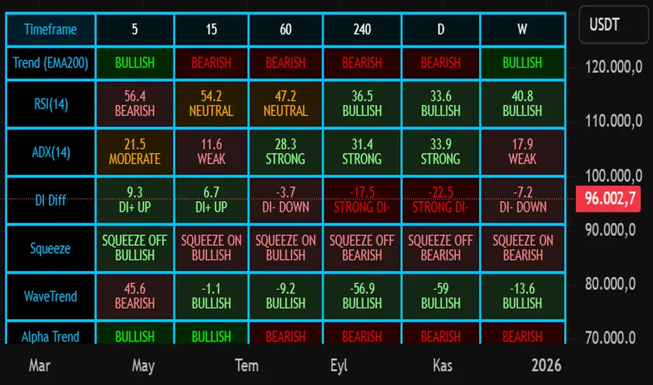
Nuh's Multi-Timeframe DashboardAll 10 indicators (EMA, RSI, ADX, RI, Squeezee, WaveTrend, Alpha Trend, SuperTrend, Stoch RSI, Vix Fix) across 7 time frames (5m, 15m, 1h, 2h, 4h, 1D, 1W) consolidated into a single table.
Algorithm Predator - ML-liteAlgorithm Predator - ML-lite
This indicator combines four specialized trading agents with an adaptive multi-armed bandit selection system to identify high-probability trade setups. It is designed for swing and intraday traders who want systematic signal generation based on institutional order flow patterns , momentum exhaustion , liquidity dynamics , and statistical mean reversion .
Core Architecture
Why These Components Are Combined:
The script addresses a fundamental challenge in algorithmic trading: no single detection method works consistently across all market conditions. By deploying four independent agents and using reinforcement learning algorithms to select or blend their outputs, the system adapts to changing market regimes without manual intervention.
The Four Trading Agents
1. Spoofing Detector Agent 🎭
Detects iceberg orders through persistent volume at similar price levels over 5 bars
Identifies spoofing patterns via asymmetric wick analysis (wicks exceeding 60% of bar range with volume >1.8× average)
Monitors order clustering using simplified Hawkes process intensity tracking (exponential decay model)
Signal Logic: Contrarian—fades false breakouts caused by institutional manipulation
Best Markets: Consolidations, institutional trading windows, low-liquidity hours
2. Exhaustion Detector Agent ⚡
Calculates RSI divergence between price movement and momentum indicator over 5-bar window
Detects VWAP exhaustion (price at 2σ bands with declining volume)
Uses VPIN reversals (volume-based toxic flow dissipation) to identify momentum failure
Signal Logic: Counter-trend—enters when momentum extreme shows weakness
Best Markets: Trending markets reaching climax points, over-extended moves
3. Liquidity Void Detector Agent 💧
Measures Bollinger Band squeeze (width <60% of 50-period average)
Identifies stop hunts via 20-bar high/low penetration with immediate reversal and volume spike
Detects hidden liquidity absorption (volume >2× average with range <0.3× ATR)
Signal Logic: Breakout anticipation—enters after liquidity grab but before main move
Best Markets: Range-bound pre-breakout, volatility compression zones
4. Mean Reversion Agent 📊
Calculates price z-scores relative to 50-period SMA and standard deviation (triggers at ±2σ)
Implements Ornstein-Uhlenbeck process scoring (mean-reverting stochastic model)
Uses entropy analysis to detect algorithmic trading patterns (low entropy <0.25 = high predictability)
Signal Logic: Statistical reversion—enters when price deviates significantly from statistical equilibrium
Best Markets: Range-bound, low-volatility, algorithmically-dominated instruments
Adaptive Selection: Multi-Armed Bandit System
The script implements four reinforcement learning algorithms to dynamically select or blend agents based on performance:
Thompson Sampling (Default - Recommended):
Uses Bayesian inference with beta distributions (tracks alpha/beta parameters per agent)
Balances exploration (trying underused agents) vs. exploitation (using proven winners)
Each agent's win/loss history informs its selection probability
Lite Approximation: Uses pseudo-random sampling from price/volume noise instead of true random number generation
UCB1 (Upper Confidence Bound):
Calculates confidence intervals using: average_reward + sqrt(2 × ln(total_pulls) / agent_pulls)
Deterministic algorithm favoring agents with high uncertainty (potential upside)
More conservative than Thompson Sampling
Epsilon-Greedy:
Exploits best-performing agent (1-ε)% of the time
Explores randomly ε% of the time (default 10%, configurable 1-50%)
Simple, transparent, easily tuned via epsilon parameter
Gradient Bandit:
Uses softmax probability distribution over agent preference weights
Updates weights via gradient ascent based on rewards
Best for Blend mode where all agents contribute
Selection Modes:
Switch Mode: Uses only the selected agent's signal (clean, decisive)
Blend Mode: Combines all agents using exponentially weighted confidence scores controlled by temperature parameter (smooth, diversified)
Lock Agent Feature:
Optional manual override to force one specific agent
Useful after identifying which agent dominates your specific instrument
Only applies in Switch mode
Four choices: Spoofing Detector, Exhaustion Detector, Liquidity Void, Mean Reversion
Memory System
Dual-Layer Architecture:
Short-Term Memory: Stores last 20 trade outcomes per agent (configurable 10-50)
Long-Term Memory: Stores episode averages when short-term reaches transfer threshold (configurable 5-20 bars)
Memory Boost Mechanism: Recent performance modulates agent scores by up to ±20%
Episode Transfer: When an agent accumulates sufficient results, averages are condensed into long-term storage
Persistence: Manual restoration of learned parameters via input fields (alpha, beta, weights, microstructure thresholds)
How Memory Works:
Agent generates signal → outcome tracked after 8 bars (performance horizon)
Result stored in short-term memory (win = 1.0, loss = 0.0)
Short-term average influences agent's future scores (positive feedback loop)
After threshold met (default 10 results), episode averaged into long-term storage
Long-term patterns (weighted 30%) + short-term patterns (weighted 70%) = total memory boost
Market Microstructure Analysis
These advanced metrics quantify institutional order flow dynamics:
Order Flow Toxicity (Simplified VPIN):
Measures buy/sell volume imbalance over 20 bars: |buy_vol - sell_vol| / (buy_vol + sell_vol)
Detects informed trading activity (institutional players with non-public information)
Values >0.4 indicate "toxic flow" (informed traders active)
Lite Approximation: Uses simple open/close heuristic instead of tick-by-tick trade classification
Price Impact Analysis (Simplified Kyle's Lambda):
Measures market impact efficiency: |price_change_10| / sqrt(volume_sum_10)
Low values = large orders with minimal price impact ( stealth accumulation )
High values = retail-dominated moves with high slippage
Lite Approximation: Uses simplified denominator instead of regression-based signed order flow
Market Randomness (Entropy Analysis):
Counts unique price changes over 20 bars / 20
Measures market predictability
High entropy (>0.6) = human-driven, chaotic price action
Low entropy (<0.25) = algorithmic trading dominance (predictable patterns)
Lite Approximation: Simple ratio instead of true Shannon entropy H(X) = -Σ p(x)·log₂(p(x))
Order Clustering (Simplified Hawkes Process):
Tracks self-exciting event intensity (coordinated order activity)
Decays at 0.9× per bar, spikes +1.0 when volume >1.5× average
High intensity (>0.7) indicates clustering (potential spoofing/accumulation)
Lite Approximation: Simple exponential decay instead of full λ(t) = μ + Σ α·exp(-β(t-tᵢ)) with MLE
Signal Generation Process
Multi-Stage Validation:
Stage 1: Agent Scoring
Each agent calculates internal score based on its detection criteria
Scores must exceed agent-specific threshold (adjusted by sensitivity multiplier)
Agent outputs: Signal direction (+1/-1/0) and Confidence level (0.0-1.0)
Stage 2: Memory Boost
Agent scores multiplied by memory boost factor (0.8-1.2 based on recent performance)
Successful agents get amplified, failing agents get dampened
Stage 3: Bandit Selection/Blending
If Adaptive Mode ON:
Switch: Bandit selects single best agent, uses only its signal
Blend: All agents combined using softmax-weighted confidence scores
If Adaptive Mode OFF:
Traditional consensus voting with confidence-squared weighting
Signal fires when consensus exceeds threshold (default 70%)
Stage 4: Confirmation Filter
Raw signal must repeat for consecutive bars (default 3, configurable 2-4)
Minimum confidence threshold: 0.25 (25%) enforced regardless of mode
Trend alignment check: Long signals require trend_score ≥ -2, Short signals require trend_score ≤ 2
Stage 5: Cooldown Enforcement
Minimum bars between signals (default 10, configurable 5-15)
Prevents over-trading during choppy conditions
Stage 6: Performance Tracking
After 8 bars (performance horizon), signal outcome evaluated
Win = price moved in signal direction, Loss = price moved against
Results fed back into memory and bandit statistics
Trading Modes (Presets)
Pre-configured parameter sets:
Conservative: 85% consensus, 4 confirmations, 15-bar cooldown
Expected: 60-70% win rate, 3-8 signals/week
Best for: Swing trading, capital preservation, beginners
Balanced: 70% consensus, 3 confirmations, 10-bar cooldown
Expected: 55-65% win rate, 8-15 signals/week
Best for: Day trading, most traders, general use
Aggressive: 60% consensus, 2 confirmations, 5-bar cooldown
Expected: 50-58% win rate, 15-30 signals/week
Best for: Scalping, high-frequency trading, active management
Elite: 75% consensus, 3 confirmations, 12-bar cooldown
Expected: 58-68% win rate, 5-12 signals/week
Best for: Selective trading, high-conviction setups
Adaptive: 65% consensus, 2 confirmations, 8-bar cooldown
Expected: Varies based on learning
Best for: Experienced users leveraging bandit system
How to Use
1. Initial Setup (5 Minutes):
Select Trading Mode matching your style (start with Balanced)
Enable Adaptive Learning (recommended for automatic agent selection)
Choose Thompson Sampling algorithm (best all-around performance)
Keep Microstructure Metrics enabled for liquid instruments (>100k daily volume)
2. Agent Tuning (Optional):
Adjust Agent Sensitivity multipliers (0.5-2.0):
<0.8 = Highly selective (fewer signals, higher quality)
0.9-1.2 = Balanced (recommended starting point)
1.3 = Aggressive (more signals, lower individual quality)
Monitor dashboard for 20-30 signals to identify dominant agent
If one agent consistently outperforms, consider using Lock Agent feature
3. Bandit Configuration (Advanced):
Blend Temperature (0.1-2.0):
0.3 = Sharp decisions (best agent dominates)
0.5 = Balanced (default)
1.0+ = Smooth (equal weighting, democratic)
Memory Decay (0.8-0.99):
0.90 = Fast adaptation (volatile markets)
0.95 = Balanced (most instruments)
0.97+ = Long memory (stable trends)
4. Signal Interpretation:
Green triangle (▲): Long signal confirmed
Red triangle (▼): Short signal confirmed
Dashboard shows:
Active agent (highlighted row with ► marker)
Win rate per agent (green >60%, yellow 40-60%, red <40%)
Confidence bars (█████ = maximum confidence)
Memory size (short-term buffer count)
Colored zones display:
Entry level (current close)
Stop-loss (1.5× ATR)
Take-profit 1 (2.0× ATR)
Take-profit 2 (3.5× ATR)
5. Risk Management:
Never risk >1-2% per signal (use ATR-based stops)
Signals are entry triggers, not complete strategies
Combine with your own market context analysis
Consider fundamental catalysts and news events
Use "Confirming" status to prepare entries (not to enter early)
6. Memory Persistence (Optional):
After 50-100 trades, check Memory Export Panel
Record displayed alpha/beta/weight values for each agent
Record VPIN and Kyle threshold values
Enable "Restore From Memory" and input saved values to continue learning
Useful when switching timeframes or restarting indicator
Visual Components
On-Chart Elements:
Spectral Layers: EMA8 ± 0.5 ATR bands (dynamic support/resistance, colored by trend)
Energy Radiance: Multi-layer glow boxes at signal points (intensity scales with confidence, configurable 1-5 layers)
Probability Cones: Projected price paths with uncertainty wedges (15-bar projection, width = confidence × ATR)
Connection Lines: Links sequential signals (solid = same direction continuation, dotted = reversal)
Kill Zones: Risk/reward boxes showing entry, stop-loss, and dual take-profit targets
Signal Markers: Triangle up/down at validated entry points
Dashboard (Configurable Position & Size):
Regime Indicator: 4-level trend classification (Strong Bull/Bear, Weak Bull/Bear)
Mode Status: Shows active system (Adaptive Blend, Locked Agent, or Consensus)
Agent Performance Table: Real-time win%, confidence, and memory stats
Order Flow Metrics: Toxicity and impact indicators (when microstructure enabled)
Signal Status: Current state (Long/Short/Confirming/Waiting) with confirmation progress
Memory Panel (Configurable Position & Size):
Live Parameter Export: Alpha, beta, and weight values per agent
Adaptive Thresholds: Current VPIN sensitivity and Kyle threshold
Save Reminder: Visual indicator if parameters should be recorded
What Makes This Original
This script's originality lies in three key innovations:
1. Genuine Meta-Learning Framework:
Unlike traditional indicator mashups that simply display multiple signals, this implements authentic reinforcement learning (multi-armed bandits) to learn which detection method works best in current conditions. The Thompson Sampling implementation with beta distribution tracking (alpha for successes, beta for failures) is statistically rigorous and adapts continuously. This is not post-hoc optimization—it's real-time learning.
2. Episodic Memory Architecture with Transfer Learning:
The dual-layer memory system mimics human learning patterns:
Short-term memory captures recent performance (recency bias)
Long-term memory preserves historical patterns (experience)
Automatic transfer mechanism consolidates knowledge
Memory boost creates positive feedback loops (successful strategies become stronger)
This architecture allows the system to adapt without retraining , unlike static ML models that require batch updates.
3. Institutional Microstructure Integration:
Combines retail-focused technical analysis (RSI, Bollinger Bands, VWAP) with institutional-grade microstructure metrics (VPIN, Kyle's Lambda, Hawkes processes) typically found in academic finance literature and professional trading systems, not standard retail platforms. While simplified for Pine Script constraints, these metrics provide insight into informed vs. uninformed trading , a dimension entirely absent from traditional technical analysis.
Mashup Justification:
The four agents are combined specifically for risk diversification across failure modes:
Spoofing Detector: Prevents false breakout losses from manipulation
Exhaustion Detector: Prevents chasing extended trends into reversals
Liquidity Void: Exploits volatility compression (different regime than trending)
Mean Reversion: Provides mathematical anchoring when patterns fail
The bandit system ensures the optimal tool is automatically selected for each market situation, rather than requiring manual interpretation of conflicting signals.
Why "ML-lite"? Simplifications and Approximations
This is the "lite" version due to necessary simplifications for Pine Script execution:
1. Simplified VPIN Calculation:
Academic Implementation: True VPIN uses volume bucketing (fixed-volume bars) and tick-by-tick buy/sell classification via Lee-Ready algorithm or exchange-provided trade direction flags
This Implementation: 20-bar rolling window with simple open/close heuristic (close > open = buy volume)
Impact: May misclassify volume during ranging/choppy markets; works best in directional moves
2. Pseudo-Random Sampling:
Academic Implementation: Thompson Sampling requires true random number generation from beta distributions using inverse transform sampling or acceptance-rejection methods
This Implementation: Deterministic pseudo-randomness derived from price and volume decimal digits: (close × 100 - floor(close × 100)) + (volume % 100) / 100
Impact: Not cryptographically random; may have subtle biases in specific price ranges; provides sufficient variation for agent selection
3. Hawkes Process Approximation:
Academic Implementation: Full Hawkes process uses maximum likelihood estimation with exponential kernels: λ(t) = μ + Σ α·exp(-β(t-tᵢ)) fitted via iterative optimization
This Implementation: Simple exponential decay (0.9 multiplier) with binary event triggers (volume spike = event)
Impact: Captures self-exciting property but lacks parameter optimization; fixed decay rate may not suit all instruments
4. Kyle's Lambda Simplification:
Academic Implementation: Estimated via regression of price impact on signed order flow over multiple time intervals: Δp = λ × Δv + ε
This Implementation: Simplified ratio: price_change / sqrt(volume_sum) without proper signed order flow or regression
Impact: Provides directional indicator of impact but not true market depth measurement; no statistical confidence intervals
5. Entropy Calculation:
Academic Implementation: True Shannon entropy requires probability distribution: H(X) = -Σ p(x)·log₂(p(x)) where p(x) is probability of each price change magnitude
This Implementation: Simple ratio of unique price changes to total observations (variety measure)
Impact: Measures diversity but not true information entropy with probability weighting; less sensitive to distribution shape
6. Memory System Constraints:
Full ML Implementation: Neural networks with backpropagation, experience replay buffers (storing state-action-reward tuples), gradient descent optimization, and eligibility traces
This Implementation: Fixed-size array queues with simple averaging; no gradient-based learning, no state representation beyond raw scores
Impact: Cannot learn complex non-linear patterns; limited to linear performance tracking
7. Limited Feature Engineering:
Advanced Implementation: Dozens of engineered features, polynomial interactions (x², x³), dimensionality reduction (PCA, autoencoders), feature selection algorithms
This Implementation: Raw agent scores and basic market metrics (RSI, ATR, volume ratio); minimal transformation
Impact: May miss subtle cross-feature interactions; relies on agent-level intelligence rather than feature combinations
8. Single-Instrument Data:
Full Implementation: Multi-asset correlation analysis (sector ETFs, currency pairs, volatility indices like VIX), lead-lag relationships, risk-on/risk-off regimes
This Implementation: Only OHLCV data from displayed instrument
Impact: Cannot incorporate broader market context; vulnerable to correlated moves across assets
9. Fixed Performance Horizon:
Full Implementation: Adaptive horizon based on trade duration, volatility regime, or profit target achievement
This Implementation: Fixed 8-bar evaluation window
Impact: May evaluate too early in slow markets or too late in fast markets; one-size-fits-all approach
Performance Impact Summary:
These simplifications make the script:
✅ Faster: Executes in milliseconds vs. seconds (or minutes) for full academic implementations
✅ More Accessible: Runs on any TradingView plan without external data feeds, APIs, or compute servers
✅ More Transparent: All calculations visible in Pine Script (no black-box compiled models)
✅ Lower Resource Usage: <500 bars lookback, minimal memory footprint
⚠️ Less Precise: Approximations may reduce statistical edge by 5-15% vs. academic implementations
⚠️ Limited Scope: Cannot capture tick-level dynamics, multi-order-book interactions, or cross-asset flows
⚠️ Fixed Parameters: Some thresholds hardcoded rather than dynamically optimized
When to Upgrade to Full Implementation:
Consider professional Python/C++ versions with institutional data feeds if:
Trading with >$100K capital where precision differences materially impact returns
Operating in microsecond-competitive environments (HFT, market making)
Requiring regulatory-grade audit trails and reproducibility
Backtesting with tick-level precision for strategy validation
Need true real-time adaptation with neural network-based learning
For retail swing/day trading and position management, these approximations provide sufficient signal quality while maintaining usability, transparency, and accessibility. The core logic—multi-agent detection with adaptive selection—remains intact.
Technical Notes
All calculations use standard Pine Script built-in functions ( ta.ema, ta.atr, ta.rsi, ta.bb, ta.sma, ta.stdev, ta.vwap )
VPIN and Kyle's Lambda use simplified formulas optimized for OHLCV data (see "Lite" section above)
Thompson Sampling uses pseudo-random noise from price/volume decimal digits for beta distribution sampling
No repainting: All calculations use confirmed bar data (no forward-looking)
Maximum lookback: 500 bars (set via max_bars_back parameter)
Performance evaluation: 8-bar forward-looking window for reward calculation (clearly disclosed)
Confidence threshold: Minimum 0.25 (25%) enforced on all signals
Memory arrays: Dynamic sizing with FIFO queue management
Limitations and Disclaimers
Not Predictive: This indicator identifies patterns in historical data. It cannot predict future price movements with certainty.
Requires Human Judgment: Signals are entry triggers, not complete trading strategies. Must be confirmed with your own analysis, risk management rules, and market context.
Learning Period Required: The adaptive system requires 50-100 bars minimum to build statistically meaningful performance data for bandit algorithms.
Overfitting Risk: Restoring memory parameters from one market regime to a drastically different regime (e.g., low volatility to high volatility) may cause poor initial performance until system re-adapts.
Approximation Limitations: Simplified calculations (see "Lite" section) may underperform academic implementations by 5-15% in highly efficient markets.
No Guarantee of Profit: Past performance, whether backtested or live-traded, does not guarantee future performance. All trading involves risk of loss.
Forward-Looking Bias: Performance evaluation uses 8-bar forward window—this creates slight look-ahead for learning (though not for signals). Real-time performance may differ from indicator's internal statistics.
Single-Instrument Limitation: Does not account for correlations with related assets or broader market regime changes.
Recommended Settings
Timeframe: 15-minute to 4-hour charts (sufficient volatility for ATR-based stops; adequate bar volume for learning)
Assets: Liquid instruments with >100k daily volume (forex majors, large-cap stocks, BTC/ETH, major indices)
Not Recommended: Illiquid small-caps, penny stocks, low-volume altcoins (microstructure metrics unreliable)
Complementary Tools: Volume profile, order book depth, market breadth indicators, fundamental catalysts
Position Sizing: Risk no more than 1-2% of capital per signal using ATR-based stop-loss
Signal Filtering: Consider external confluence (support/resistance, trendlines, round numbers, session opens)
Start With: Balanced mode, Thompson Sampling, Blend mode, default agent sensitivities (1.0)
After 30+ Signals: Review agent win rates, consider increasing sensitivity of top performers or locking to dominant agent
Alert Configuration
The script includes built-in alert conditions:
Long Signal: Fires when validated long entry confirmed
Short Signal: Fires when validated short entry confirmed
Alerts fire once per bar (after confirmation requirements met)
Set alert to "Once Per Bar Close" for reliability
Taking you to school. — Dskyz, Trade with insight. Trade with anticipation.

Quantum Rotational Field MappingQuantum Rotational Field Mapping (QRFM):
Phase Coherence Detection Through Complex-Plane Oscillator Analysis
Quantum Rotational Field Mapping applies complex-plane mathematics and phase-space analysis to oscillator ensembles, identifying high-probability trend ignition points by measuring when multiple independent oscillators achieve phase coherence. Unlike traditional multi-oscillator approaches that simply stack indicators or use boolean AND/OR logic, this system converts each oscillator into a rotating phasor (vector) in the complex plane and calculates the Coherence Index (CI) —a mathematical measure of how tightly aligned the ensemble has become—then generates signals only when alignment, phase direction, and pairwise entanglement all converge.
The indicator combines three mathematical frameworks: phasor representation using analytic signal theory to extract phase and amplitude from each oscillator, coherence measurement using vector summation in the complex plane to quantify group alignment, and entanglement analysis that calculates pairwise phase agreement across all oscillator combinations. This creates a multi-dimensional confirmation system that distinguishes between random oscillator noise and genuine regime transitions.
What Makes This Original
Complex-Plane Phasor Framework
This indicator implements classical signal processing mathematics adapted for market oscillators. Each oscillator—whether RSI, MACD, Stochastic, CCI, Williams %R, MFI, ROC, or TSI—is first normalized to a common scale, then converted into a complex-plane representation using an in-phase (I) and quadrature (Q) component. The in-phase component is the oscillator value itself, while the quadrature component is calculated as the first difference (derivative proxy), creating a velocity-aware representation.
From these components, the system extracts:
Phase (φ) : Calculated as φ = atan2(Q, I), representing the oscillator's position in its cycle (mapped to -180° to +180°)
Amplitude (A) : Calculated as A = √(I² + Q²), representing the oscillator's strength or conviction
This mathematical approach is fundamentally different from simply reading oscillator values. A phasor captures both where an oscillator is in its cycle (phase angle) and how strongly it's expressing that position (amplitude). Two oscillators can have the same value but be in opposite phases of their cycles—traditional analysis would see them as identical, while QRFM sees them as 180° out of phase (contradictory).
Coherence Index Calculation
The core innovation is the Coherence Index (CI) , borrowed from physics and signal processing. When you have N oscillators, each with phase φₙ, you can represent each as a unit vector in the complex plane: e^(iφₙ) = cos(φₙ) + i·sin(φₙ).
The CI measures what happens when you sum all these vectors:
Resultant Vector : R = Σ e^(iφₙ) = Σ cos(φₙ) + i·Σ sin(φₙ)
Coherence Index : CI = |R| / N
Where |R| is the magnitude of the resultant vector and N is the number of active oscillators.
The CI ranges from 0 to 1:
CI = 1.0 : Perfect coherence—all oscillators have identical phase angles, vectors point in the same direction, creating maximum constructive interference
CI = 0.0 : Complete decoherence—oscillators are randomly distributed around the circle, vectors cancel out through destructive interference
0 < CI < 1 : Partial alignment—some clustering with some scatter
This is not a simple average or correlation. The CI captures phase synchronization across the entire ensemble simultaneously. When oscillators phase-lock (align their cycles), the CI spikes regardless of their individual values. This makes it sensitive to regime transitions that traditional indicators miss.
Dominant Phase and Direction Detection
Beyond measuring alignment strength, the system calculates the dominant phase of the ensemble—the direction the resultant vector points:
Dominant Phase : φ_dom = atan2(Σ sin(φₙ), Σ cos(φₙ))
This gives the "average direction" of all oscillator phases, mapped to -180° to +180°:
+90° to -90° (right half-plane): Bullish phase dominance
+90° to +180° or -90° to -180° (left half-plane): Bearish phase dominance
The combination of CI magnitude (coherence strength) and dominant phase angle (directional bias) creates a two-dimensional signal space. High CI alone is insufficient—you need high CI plus dominant phase pointing in a tradeable direction. This dual requirement is what separates QRFM from simple oscillator averaging.
Entanglement Matrix and Pairwise Coherence
While the CI measures global alignment, the entanglement matrix measures local pairwise relationships. For every pair of oscillators (i, j), the system calculates:
E(i,j) = |cos(φᵢ - φⱼ)|
This represents the phase agreement between oscillators i and j:
E = 1.0 : Oscillators are in-phase (0° or 360° apart)
E = 0.0 : Oscillators are in quadrature (90° apart, orthogonal)
E between 0 and 1 : Varying degrees of alignment
The system counts how many oscillator pairs exceed a user-defined entanglement threshold (e.g., 0.7). This entangled pairs count serves as a confirmation filter: signals require not just high global CI, but also a minimum number of strong pairwise agreements. This prevents false ignitions where CI is high but driven by only two oscillators while the rest remain scattered.
The entanglement matrix creates an N×N symmetric matrix that can be visualized as a web—when many cells are bright (high E values), the ensemble is highly interconnected. When cells are dark, oscillators are moving independently.
Phase-Lock Tolerance Mechanism
A complementary confirmation layer is the phase-lock detector . This calculates the maximum phase spread across all oscillators:
For all pairs (i,j), compute angular distance: Δφ = |φᵢ - φⱼ|, wrapping at 180°
Max Spread = maximum Δφ across all pairs
If max spread < user threshold (e.g., 35°), the ensemble is considered phase-locked —all oscillators are within a narrow angular band.
This differs from entanglement: entanglement measures pairwise cosine similarity (magnitude of alignment), while phase-lock measures maximum angular deviation (tightness of clustering). Both must be satisfied for the highest-conviction signals.
Multi-Layer Visual Architecture
QRFM includes six visual components that represent the same underlying mathematics from different perspectives:
Circular Orbit Plot : A polar coordinate grid showing each oscillator as a vector from origin to perimeter. Angle = phase, radius = amplitude. This is a real-time snapshot of the complex plane. When vectors converge (point in similar directions), coherence is high. When scattered randomly, coherence is low. Users can see phase alignment forming before CI numerically confirms it.
Phase-Time Heat Map : A 2D matrix with rows = oscillators and columns = time bins. Each cell is colored by the oscillator's phase at that time (using a gradient where color hue maps to angle). Horizontal color bands indicate sustained phase alignment over time. Vertical color bands show moments when all oscillators shared the same phase (ignition points). This provides historical pattern recognition.
Entanglement Web Matrix : An N×N grid showing E(i,j) for all pairs. Cells are colored by entanglement strength—bright yellow/gold for high E, dark gray for low E. This reveals which oscillators are driving coherence and which are lagging. For example, if RSI and MACD show high E but Stochastic shows low E with everything, Stochastic is the outlier.
Quantum Field Cloud : A background color overlay on the price chart. Color (green = bullish, red = bearish) is determined by dominant phase. Opacity is determined by CI—high CI creates dense, opaque cloud; low CI creates faint, nearly invisible cloud. This gives an atmospheric "feel" for regime strength without looking at numbers.
Phase Spiral : A smoothed plot of dominant phase over recent history, displayed as a curve that wraps around price. When the spiral is tight and rotating steadily, the ensemble is in coherent rotation (trending). When the spiral is loose or erratic, coherence is breaking down.
Dashboard : A table showing real-time metrics: CI (as percentage), dominant phase (in degrees with directional arrow), field strength (CI × average amplitude), entangled pairs count, phase-lock status (locked/unlocked), quantum state classification ("Ignition", "Coherent", "Collapse", "Chaos"), and collapse risk (recent CI change normalized to 0-100%).
Each component is independently toggleable, allowing users to customize their workspace. The orbit plot is the most essential—it provides intuitive, visual feedback on phase alignment that no numerical dashboard can match.
Core Components and How They Work Together
1. Oscillator Normalization Engine
The foundation is creating a common measurement scale. QRFM supports eight oscillators:
RSI : Normalized from to using overbought/oversold levels (70, 30) as anchors
MACD Histogram : Normalized by dividing by rolling standard deviation, then clamped to
Stochastic %K : Normalized from using (80, 20) anchors
CCI : Divided by 200 (typical extreme level), clamped to
Williams %R : Normalized from using (-20, -80) anchors
MFI : Normalized from using (80, 20) anchors
ROC : Divided by 10, clamped to
TSI : Divided by 50, clamped to
Each oscillator can be individually enabled/disabled. Only active oscillators contribute to phase calculations. The normalization removes scale differences—a reading of +0.8 means "strongly bullish" regardless of whether it came from RSI or TSI.
2. Analytic Signal Construction
For each active oscillator at each bar, the system constructs the analytic signal:
In-Phase (I) : The normalized oscillator value itself
Quadrature (Q) : The bar-to-bar change in the normalized value (first derivative approximation)
This creates a 2D representation: (I, Q). The phase is extracted as:
φ = atan2(Q, I) × (180 / π)
This maps the oscillator to a point on the unit circle. An oscillator at the same value but rising (positive Q) will have a different phase than one that is falling (negative Q). This velocity-awareness is critical—it distinguishes between "at resistance and stalling" versus "at resistance and breaking through."
The amplitude is extracted as:
A = √(I² + Q²)
This represents the distance from origin in the (I, Q) plane. High amplitude means the oscillator is far from neutral (strong conviction). Low amplitude means it's near zero (weak/transitional state).
3. Coherence Calculation Pipeline
For each bar (or every Nth bar if phase sample rate > 1 for performance):
Step 1 : Extract phase φₙ for each of the N active oscillators
Step 2 : Compute complex exponentials: Zₙ = e^(i·φₙ·π/180) = cos(φₙ·π/180) + i·sin(φₙ·π/180)
Step 3 : Sum the complex exponentials: R = Σ Zₙ = (Σ cos φₙ) + i·(Σ sin φₙ)
Step 4 : Calculate magnitude: |R| = √
Step 5 : Normalize by count: CI_raw = |R| / N
Step 6 : Smooth the CI: CI = SMA(CI_raw, smoothing_window)
The smoothing step (default 2 bars) removes single-bar noise spikes while preserving structural coherence changes. Users can adjust this to control reactivity versus stability.
The dominant phase is calculated as:
φ_dom = atan2(Σ sin φₙ, Σ cos φₙ) × (180 / π)
This is the angle of the resultant vector R in the complex plane.
4. Entanglement Matrix Construction
For all unique pairs of oscillators (i, j) where i < j:
Step 1 : Get phases φᵢ and φⱼ
Step 2 : Compute phase difference: Δφ = φᵢ - φⱼ (in radians)
Step 3 : Calculate entanglement: E(i,j) = |cos(Δφ)|
Step 4 : Store in symmetric matrix: matrix = matrix = E(i,j)
The matrix is then scanned: count how many E(i,j) values exceed the user-defined threshold (default 0.7). This count is the entangled pairs metric.
For visualization, the matrix is rendered as an N×N table where cell brightness maps to E(i,j) intensity.
5. Phase-Lock Detection
Step 1 : For all unique pairs (i, j), compute angular distance: Δφ = |φᵢ - φⱼ|
Step 2 : Wrap angles: if Δφ > 180°, set Δφ = 360° - Δφ
Step 3 : Find maximum: max_spread = max(Δφ) across all pairs
Step 4 : Compare to tolerance: phase_locked = (max_spread < tolerance)
If phase_locked is true, all oscillators are within the specified angular cone (e.g., 35°). This is a boolean confirmation filter.
6. Signal Generation Logic
Signals are generated through multi-layer confirmation:
Long Ignition Signal :
CI crosses above ignition threshold (e.g., 0.80)
AND dominant phase is in bullish range (-90° < φ_dom < +90°)
AND phase_locked = true
AND entangled_pairs >= minimum threshold (e.g., 4)
Short Ignition Signal :
CI crosses above ignition threshold
AND dominant phase is in bearish range (φ_dom < -90° OR φ_dom > +90°)
AND phase_locked = true
AND entangled_pairs >= minimum threshold
Collapse Signal :
CI at bar minus CI at current bar > collapse threshold (e.g., 0.55)
AND CI at bar was above 0.6 (must collapse from coherent state, not from already-low state)
These are strict conditions. A high CI alone does not generate a signal—dominant phase must align with direction, oscillators must be phase-locked, and sufficient pairwise entanglement must exist. This multi-factor gating dramatically reduces false signals compared to single-condition triggers.
Calculation Methodology
Phase 1: Oscillator Computation and Normalization
On each bar, the system calculates the raw values for all enabled oscillators using standard Pine Script functions:
RSI: ta.rsi(close, length)
MACD: ta.macd() returning histogram component
Stochastic: ta.stoch() smoothed with ta.sma()
CCI: ta.cci(close, length)
Williams %R: ta.wpr(length)
MFI: ta.mfi(hlc3, length)
ROC: ta.roc(close, length)
TSI: ta.tsi(close, short, long)
Each raw value is then passed through a normalization function:
normalize(value, overbought_level, oversold_level) = 2 × (value - oversold) / (overbought - oversold) - 1
This maps the oscillator's typical range to , where -1 represents extreme bearish, 0 represents neutral, and +1 represents extreme bullish.
For oscillators without fixed ranges (MACD, ROC, TSI), statistical normalization is used: divide by a rolling standard deviation or fixed divisor, then clamp to .
Phase 2: Phasor Extraction
For each normalized oscillator value val:
I = val (in-phase component)
Q = val - val (quadrature component, first difference)
Phase calculation:
phi_rad = atan2(Q, I)
phi_deg = phi_rad × (180 / π)
Amplitude calculation:
A = √(I² + Q²)
These values are stored in arrays: osc_phases and osc_amps for each oscillator n.
Phase 3: Complex Summation and Coherence
Initialize accumulators:
sum_cos = 0
sum_sin = 0
For each oscillator n = 0 to N-1:
phi_rad = osc_phases × (π / 180)
sum_cos += cos(phi_rad)
sum_sin += sin(phi_rad)
Resultant magnitude:
resultant_mag = √(sum_cos² + sum_sin²)
Coherence Index (raw):
CI_raw = resultant_mag / N
Smoothed CI:
CI = SMA(CI_raw, smoothing_window)
Dominant phase:
phi_dom_rad = atan2(sum_sin, sum_cos)
phi_dom_deg = phi_dom_rad × (180 / π)
Phase 4: Entanglement Matrix Population
For i = 0 to N-2:
For j = i+1 to N-1:
phi_i = osc_phases × (π / 180)
phi_j = osc_phases × (π / 180)
delta_phi = phi_i - phi_j
E = |cos(delta_phi)|
matrix_index_ij = i × N + j
matrix_index_ji = j × N + i
entangle_matrix = E
entangle_matrix = E
if E >= threshold:
entangled_pairs += 1
The matrix uses flat array storage with index mapping: index(row, col) = row × N + col.
Phase 5: Phase-Lock Check
max_spread = 0
For i = 0 to N-2:
For j = i+1 to N-1:
delta = |osc_phases - osc_phases |
if delta > 180:
delta = 360 - delta
max_spread = max(max_spread, delta)
phase_locked = (max_spread < tolerance)
Phase 6: Signal Evaluation
Ignition Long :
ignition_long = (CI crosses above threshold) AND
(phi_dom > -90 AND phi_dom < 90) AND
phase_locked AND
(entangled_pairs >= minimum)
Ignition Short :
ignition_short = (CI crosses above threshold) AND
(phi_dom < -90 OR phi_dom > 90) AND
phase_locked AND
(entangled_pairs >= minimum)
Collapse :
CI_prev = CI
collapse = (CI_prev - CI > collapse_threshold) AND (CI_prev > 0.6)
All signals are evaluated on bar close. The crossover and crossunder functions ensure signals fire only once when conditions transition from false to true.
Phase 7: Field Strength and Visualization Metrics
Average Amplitude :
avg_amp = (Σ osc_amps ) / N
Field Strength :
field_strength = CI × avg_amp
Collapse Risk (for dashboard):
collapse_risk = (CI - CI) / max(CI , 0.1)
collapse_risk_pct = clamp(collapse_risk × 100, 0, 100)
Quantum State Classification :
if (CI > threshold AND phase_locked):
state = "Ignition"
else if (CI > 0.6):
state = "Coherent"
else if (collapse):
state = "Collapse"
else:
state = "Chaos"
Phase 8: Visual Rendering
Orbit Plot : For each oscillator, convert polar (phase, amplitude) to Cartesian (x, y) for grid placement:
radius = amplitude × grid_center × 0.8
x = radius × cos(phase × π/180)
y = radius × sin(phase × π/180)
col = center + x (mapped to grid coordinates)
row = center - y
Heat Map : For each oscillator row and time column, retrieve historical phase value at lookback = (columns - col) × sample_rate, then map phase to color using a hue gradient.
Entanglement Web : Render matrix as table cell with background color opacity = E(i,j).
Field Cloud : Background color = (phi_dom > -90 AND phi_dom < 90) ? green : red, with opacity = mix(min_opacity, max_opacity, CI).
All visual components render only on the last bar (barstate.islast) to minimize computational overhead.
How to Use This Indicator
Step 1 : Apply QRFM to your chart. It works on all timeframes and asset classes, though 15-minute to 4-hour timeframes provide the best balance of responsiveness and noise reduction.
Step 2 : Enable the dashboard (default: top right) and the circular orbit plot (default: middle left). These are your primary visual feedback tools.
Step 3 : Optionally enable the heat map, entanglement web, and field cloud based on your preference. New users may find all visuals overwhelming; start with dashboard + orbit plot.
Step 4 : Observe for 50-100 bars to let the indicator establish baseline coherence patterns. Markets have different "normal" CI ranges—some instruments naturally run higher or lower coherence.
Understanding the Circular Orbit Plot
The orbit plot is a polar grid showing oscillator vectors in real-time:
Center point : Neutral (zero phase and amplitude)
Each vector : A line from center to a point on the grid
Vector angle : The oscillator's phase (0° = right/east, 90° = up/north, 180° = left/west, -90° = down/south)
Vector length : The oscillator's amplitude (short = weak signal, long = strong signal)
Vector label : First letter of oscillator name (R = RSI, M = MACD, etc.)
What to watch :
Convergence : When all vectors cluster in one quadrant or sector, CI is rising and coherence is forming. This is your pre-signal warning.
Scatter : When vectors point in random directions (360° spread), CI is low and the market is in a non-trending or transitional regime.
Rotation : When the cluster rotates smoothly around the circle, the ensemble is in coherent oscillation—typically seen during steady trends.
Sudden flips : When the cluster rapidly jumps from one side to the opposite (e.g., +90° to -90°), a phase reversal has occurred—often coinciding with trend reversals.
Example: If you see RSI, MACD, and Stochastic all pointing toward 45° (northeast) with long vectors, while CCI, TSI, and ROC point toward 40-50° as well, coherence is high and dominant phase is bullish. Expect an ignition signal if CI crosses threshold.
Reading Dashboard Metrics
The dashboard provides numerical confirmation of what the orbit plot shows visually:
CI : Displays as 0-100%. Above 70% = high coherence (strong regime), 40-70% = moderate, below 40% = low (poor conditions for trend entries).
Dom Phase : Angle in degrees with directional arrow. ⬆ = bullish bias, ⬇ = bearish bias, ⬌ = neutral.
Field Strength : CI weighted by amplitude. High values (> 0.6) indicate not just alignment but strong alignment.
Entangled Pairs : Count of oscillator pairs with E > threshold. Higher = more confirmation. If minimum is set to 4, you need at least 4 pairs entangled for signals.
Phase Lock : 🔒 YES (all oscillators within tolerance) or 🔓 NO (spread too wide).
State : Real-time classification:
🚀 IGNITION: CI just crossed threshold with phase-lock
⚡ COHERENT: CI is high and stable
💥 COLLAPSE: CI has dropped sharply
🌀 CHAOS: Low CI, scattered phases
Collapse Risk : 0-100% scale based on recent CI change. Above 50% warns of imminent breakdown.
Interpreting Signals
Long Ignition (Blue Triangle Below Price) :
Occurs when CI crosses above threshold (e.g., 0.80)
Dominant phase is in bullish range (-90° to +90°)
All oscillators are phase-locked (within tolerance)
Minimum entangled pairs requirement met
Interpretation : The oscillator ensemble has transitioned from disorder to coherent bullish alignment. This is a high-probability long entry point. The multi-layer confirmation (CI + phase direction + lock + entanglement) ensures this is not a single-oscillator whipsaw.
Short Ignition (Red Triangle Above Price) :
Same conditions as long, but dominant phase is in bearish range (< -90° or > +90°)
Interpretation : Coherent bearish alignment has formed. High-probability short entry.
Collapse (Circles Above and Below Price) :
CI has dropped by more than the collapse threshold (e.g., 0.55) over a 5-bar window
CI was previously above 0.6 (collapsing from coherent state)
Interpretation : Phase coherence has broken down. If you are in a position, this is an exit warning. If looking to enter, stand aside—regime is transitioning.
Phase-Time Heat Map Patterns
Enable the heat map and position it at bottom right. The rows represent individual oscillators, columns represent time bins (most recent on left).
Pattern: Horizontal Color Bands
If a row (e.g., RSI) shows consistent color across columns (say, green for several bins), that oscillator has maintained stable phase over time. If all rows show horizontal bands of similar color, the entire ensemble has been phase-locked for an extended period—this is a strong trending regime.
Pattern: Vertical Color Bands
If a column (single time bin) shows all cells with the same or very similar color, that moment in time had high coherence. These vertical bands often align with ignition signals or major price pivots.
Pattern: Rainbow Chaos
If cells are random colors (red, green, yellow mixed with no pattern), coherence is low. The ensemble is scattered. Avoid trading during these periods unless you have external confirmation.
Pattern: Color Transition
If you see a row transition from red to green (or vice versa) sharply, that oscillator has phase-flipped. If multiple rows do this simultaneously, a regime change is underway.
Entanglement Web Analysis
Enable the web matrix (default: opposite corner from heat map). It shows an N×N grid where N = number of active oscillators.
Bright Yellow/Gold Cells : High pairwise entanglement. For example, if the RSI-MACD cell is bright gold, those two oscillators are moving in phase. If the RSI-Stochastic cell is bright, they are entangled as well.
Dark Gray Cells : Low entanglement. Oscillators are decorrelated or in quadrature.
Diagonal : Always marked with "—" because an oscillator is always perfectly entangled with itself.
How to use :
Scan for clustering: If most cells are bright, coherence is high across the board. If only a few cells are bright, coherence is driven by a subset (e.g., RSI and MACD are aligned, but nothing else is—weak signal).
Identify laggards: If one row/column is entirely dark, that oscillator is the outlier. You may choose to disable it or monitor for when it joins the group (late confirmation).
Watch for web formation: During low-coherence periods, the matrix is mostly dark. As coherence builds, cells begin lighting up. A sudden "web" of connections forming visually precedes ignition signals.
Trading Workflow
Step 1: Monitor Coherence Level
Check the dashboard CI metric or observe the orbit plot. If CI is below 40% and vectors are scattered, conditions are poor for trend entries. Wait.
Step 2: Detect Coherence Building
When CI begins rising (say, from 30% to 50-60%) and you notice vectors on the orbit plot starting to cluster, coherence is forming. This is your alert phase—do not enter yet, but prepare.
Step 3: Confirm Phase Direction
Check the dominant phase angle and the orbit plot quadrant where clustering is occurring:
Clustering in right half (0° to ±90°): Bullish bias forming
Clustering in left half (±90° to 180°): Bearish bias forming
Verify the dashboard shows the corresponding directional arrow (⬆ or ⬇).
Step 4: Wait for Signal Confirmation
Do not enter based on rising CI alone. Wait for the full ignition signal:
CI crosses above threshold
Phase-lock indicator shows 🔒 YES
Entangled pairs count >= minimum
Directional triangle appears on chart
This ensures all layers have aligned.
Step 5: Execute Entry
Long : Blue triangle below price appears → enter long
Short : Red triangle above price appears → enter short
Step 6: Position Management
Initial Stop : Place stop loss based on your risk management rules (e.g., recent swing low/high, ATR-based buffer).
Monitoring :
Watch the field cloud density. If it remains opaque and colored in your direction, the regime is intact.
Check dashboard collapse risk. If it rises above 50%, prepare for exit.
Monitor the orbit plot. If vectors begin scattering or the cluster flips to the opposite side, coherence is breaking.
Exit Triggers :
Collapse signal fires (circles appear)
Dominant phase flips to opposite half-plane
CI drops below 40% (coherence lost)
Price hits your profit target or trailing stop
Step 7: Post-Exit Analysis
After exiting, observe whether a new ignition forms in the opposite direction (reversal) or if CI remains low (transition to range). Use this to decide whether to re-enter, reverse, or stand aside.
Best Practices
Use Price Structure as Context
QRFM identifies when coherence forms but does not specify where price will go. Combine ignition signals with support/resistance levels, trendlines, or chart patterns. For example:
Long ignition near a major support level after a pullback: high-probability bounce
Long ignition in the middle of a range with no structure: lower probability
Multi-Timeframe Confirmation
Open QRFM on two timeframes simultaneously:
Higher timeframe (e.g., 4-hour): Use CI level to determine regime bias. If 4H CI is above 60% and dominant phase is bullish, the market is in a bullish regime.
Lower timeframe (e.g., 15-minute): Execute entries on ignition signals that align with the higher timeframe bias.
This prevents counter-trend trades and increases win rate.
Distinguish Between Regime Types
High CI, stable dominant phase (State: Coherent) : Trending market. Ignitions are continuation signals; collapses are profit-taking or reversal warnings.
Low CI, erratic dominant phase (State: Chaos) : Ranging or choppy market. Avoid ignition signals or reduce position size. Wait for coherence to establish.
Moderate CI with frequent collapses : Whipsaw environment. Use wider stops or stand aside.
Adjust Parameters to Instrument and Timeframe
Crypto/Forex (high volatility) : Lower ignition threshold (0.65-0.75), lower CI smoothing (2-3), shorter oscillator lengths (7-10).
Stocks/Indices (moderate volatility) : Standard settings (threshold 0.75-0.85, smoothing 5-7, oscillator lengths 14).
Lower timeframes (5-15 min) : Reduce phase sample rate to 1-2 for responsiveness.
Higher timeframes (daily+) : Increase CI smoothing and oscillator lengths for noise reduction.
Use Entanglement Count as Conviction Filter
The minimum entangled pairs setting controls signal strictness:
Low (1-2) : More signals, lower quality (acceptable if you have other confirmation)
Medium (3-5) : Balanced (recommended for most traders)
High (6+) : Very strict, fewer signals, highest quality
Adjust based on your trade frequency preference and risk tolerance.
Monitor Oscillator Contribution
Use the entanglement web to see which oscillators are driving coherence. If certain oscillators are consistently dark (low E with all others), they may be adding noise. Consider disabling them. For example:
On low-volume instruments, MFI may be unreliable → disable MFI
On strongly trending instruments, mean-reversion oscillators (Stochastic, RSI) may lag → reduce weight or disable
Respect the Collapse Signal
Collapse events are early warnings. Price may continue in the original direction for several bars after collapse fires, but the underlying regime has weakened. Best practice:
If in profit: Take partial or full profit on collapse
If at breakeven/small loss: Exit immediately
If collapse occurs shortly after entry: Likely a false ignition; exit to avoid drawdown
Collapses do not guarantee immediate reversals—they signal uncertainty .
Combine with Volume Analysis
If your instrument has reliable volume:
Ignitions with expanding volume: Higher conviction
Ignitions with declining volume: Weaker, possibly false
Collapses with volume spikes: Strong reversal signal
Collapses with low volume: May just be consolidation
Volume is not built into QRFM (except via MFI), so add it as external confirmation.
Observe the Phase Spiral
The spiral provides a quick visual cue for rotation consistency:
Tight, smooth spiral : Ensemble is rotating coherently (trending)
Loose, erratic spiral : Phase is jumping around (ranging or transitional)
If the spiral tightens, coherence is building. If it loosens, coherence is dissolving.
Do Not Overtrade Low-Coherence Periods
When CI is persistently below 40% and the state is "Chaos," the market is not in a regime where phase analysis is predictive. During these times:
Reduce position size
Widen stops
Wait for coherence to return
QRFM's strength is regime detection. If there is no regime, the tool correctly signals "stand aside."
Use Alerts Strategically
Set alerts for:
Long Ignition
Short Ignition
Collapse
Phase Lock (optional)
Configure alerts to "Once per bar close" to avoid intrabar repainting and noise. When an alert fires, manually verify:
Orbit plot shows clustering
Dashboard confirms all conditions
Price structure supports the trade
Do not blindly trade alerts—use them as prompts for analysis.
Ideal Market Conditions
Best Performance
Instruments :
Liquid, actively traded markets (major forex pairs, large-cap stocks, major indices, top-tier crypto)
Instruments with clear cyclical oscillator behavior (avoid extremely illiquid or manipulated markets)
Timeframes :
15-minute to 4-hour: Optimal balance of noise reduction and responsiveness
1-hour to daily: Slower, higher-conviction signals; good for swing trading
5-minute: Acceptable for scalping if parameters are tightened and you accept more noise
Market Regimes :
Trending markets with periodic retracements (where oscillators cycle through phases predictably)
Breakout environments (coherence forms before/during breakout; collapse occurs at exhaustion)
Rotational markets with clear swings (oscillators phase-lock at turning points)
Volatility :
Moderate to high volatility (oscillators have room to move through their ranges)
Stable volatility regimes (sudden VIX spikes or flash crashes may create false collapses)
Challenging Conditions
Instruments :
Very low liquidity markets (erratic price action creates unstable oscillator phases)
Heavily news-driven instruments (fundamentals may override technical coherence)
Highly correlated instruments (oscillators may all reflect the same underlying factor, reducing independence)
Market Regimes :
Deep, prolonged consolidation (oscillators remain near neutral, CI is chronically low, few signals fire)
Extreme chop with no directional bias (oscillators whipsaw, coherence never establishes)
Gap-driven markets (large overnight gaps create phase discontinuities)
Timeframes :
Sub-5-minute charts: Noise dominates; oscillators flip rapidly; coherence is fleeting and unreliable
Weekly/monthly: Oscillators move extremely slowly; signals are rare; better suited for long-term positioning than active trading
Special Cases :
During major economic releases or earnings: Oscillators may lag price or become decorrelated as fundamentals overwhelm technicals. Reduce position size or stand aside.
In extremely low-volatility environments (e.g., holiday periods): Oscillators compress to neutral, CI may be artificially high due to lack of movement, but signals lack follow-through.
Adaptive Behavior
QRFM is designed to self-adapt to poor conditions:
When coherence is genuinely absent, CI remains low and signals do not fire
When only a subset of oscillators aligns, entangled pairs count stays below threshold and signals are filtered out
When phase-lock cannot be achieved (oscillators too scattered), the lock filter prevents signals
This means the indicator will naturally produce fewer (or zero) signals during unfavorable conditions, rather than generating false signals. This is a feature —it keeps you out of low-probability trades.
Parameter Optimization by Trading Style
Scalping (5-15 Minute Charts)
Goal : Maximum responsiveness, accept higher noise
Oscillator Lengths :
RSI: 7-10
MACD: 8/17/6
Stochastic: 8-10, smooth 2-3
CCI: 14-16
Others: 8-12
Coherence Settings :
CI Smoothing Window: 2-3 bars (fast reaction)
Phase Sample Rate: 1 (every bar)
Ignition Threshold: 0.65-0.75 (lower for more signals)
Collapse Threshold: 0.40-0.50 (earlier exit warnings)
Confirmation :
Phase Lock Tolerance: 40-50° (looser, easier to achieve)
Min Entangled Pairs: 2-3 (fewer oscillators required)
Visuals :
Orbit Plot + Dashboard only (reduce screen clutter for fast decisions)
Disable heavy visuals (heat map, web) for performance
Alerts :
Enable all ignition and collapse alerts
Set to "Once per bar close"
Day Trading (15-Minute to 1-Hour Charts)
Goal : Balance between responsiveness and reliability
Oscillator Lengths :
RSI: 14 (standard)
MACD: 12/26/9 (standard)
Stochastic: 14, smooth 3
CCI: 20
Others: 10-14
Coherence Settings :
CI Smoothing Window: 3-5 bars (balanced)
Phase Sample Rate: 2-3
Ignition Threshold: 0.75-0.85 (moderate selectivity)
Collapse Threshold: 0.50-0.55 (balanced exit timing)
Confirmation :
Phase Lock Tolerance: 30-40° (moderate tightness)
Min Entangled Pairs: 4-5 (reasonable confirmation)
Visuals :
Orbit Plot + Dashboard + Heat Map or Web (choose one)
Field Cloud for regime backdrop
Alerts :
Ignition and collapse alerts
Optional phase-lock alert for advance warning
Swing Trading (4-Hour to Daily Charts)
Goal : High-conviction signals, minimal noise, fewer trades
Oscillator Lengths :
RSI: 14-21
MACD: 12/26/9 or 19/39/9 (longer variant)
Stochastic: 14-21, smooth 3-5
CCI: 20-30
Others: 14-20
Coherence Settings :
CI Smoothing Window: 5-10 bars (very smooth)
Phase Sample Rate: 3-5
Ignition Threshold: 0.80-0.90 (high bar for entry)
Collapse Threshold: 0.55-0.65 (only significant breakdowns)
Confirmation :
Phase Lock Tolerance: 20-30° (tight clustering required)
Min Entangled Pairs: 5-7 (strong confirmation)
Visuals :
All modules enabled (you have time to analyze)
Heat Map for multi-bar pattern recognition
Web for deep confirmation analysis
Alerts :
Ignition and collapse
Review manually before entering (no rush)
Position/Long-Term Trading (Daily to Weekly Charts)
Goal : Rare, very high-conviction regime shifts
Oscillator Lengths :
RSI: 21-30
MACD: 19/39/9 or 26/52/12
Stochastic: 21, smooth 5
CCI: 30-50
Others: 20-30
Coherence Settings :
CI Smoothing Window: 10-14 bars
Phase Sample Rate: 5 (every 5th bar to reduce computation)
Ignition Threshold: 0.85-0.95 (only extreme alignment)
Collapse Threshold: 0.60-0.70 (major regime breaks only)
Confirmation :
Phase Lock Tolerance: 15-25° (very tight)
Min Entangled Pairs: 6+ (broad consensus required)
Visuals :
Dashboard + Orbit Plot for quick checks
Heat Map to study historical coherence patterns
Web to verify deep entanglement
Alerts :
Ignition only (collapses are less critical on long timeframes)
Manual review with fundamental analysis overlay
Performance Optimization (Low-End Systems)
If you experience lag or slow rendering:
Reduce Visual Load :
Orbit Grid Size: 8-10 (instead of 12+)
Heat Map Time Bins: 5-8 (instead of 10+)
Disable Web Matrix entirely if not needed
Disable Field Cloud and Phase Spiral
Reduce Calculation Frequency :
Phase Sample Rate: 5-10 (calculate every 5-10 bars)
Max History Depth: 100-200 (instead of 500+)
Disable Unused Oscillators :
If you only want RSI, MACD, and Stochastic, disable the other five. Fewer oscillators = smaller matrices, faster loops.
Simplify Dashboard :
Choose "Small" dashboard size
Reduce number of metrics displayed
These settings will not significantly degrade signal quality (signals are based on bar-close calculations, which remain accurate), but will improve chart responsiveness.
Important Disclaimers
This indicator is a technical analysis tool designed to identify periods of phase coherence across an ensemble of oscillators. It is not a standalone trading system and does not guarantee profitable trades. The Coherence Index, dominant phase, and entanglement metrics are mathematical calculations applied to historical price data—they measure past oscillator behavior and do not predict future price movements with certainty.
No Predictive Guarantee : High coherence indicates that oscillators are currently aligned, which historically has coincided with trending or directional price movement. However, past alignment does not guarantee future trends. Markets can remain coherent while prices consolidate, or lose coherence suddenly due to news, liquidity changes, or other factors not captured by oscillator mathematics.
Signal Confirmation is Probabilistic : The multi-layer confirmation system (CI threshold + dominant phase + phase-lock + entanglement) is designed to filter out low-probability setups. This increases the proportion of valid signals relative to false signals, but does not eliminate false signals entirely. Users should combine QRFM with additional analysis—support and resistance levels, volume confirmation, multi-timeframe alignment, and fundamental context—before executing trades.
Collapse Signals are Warnings, Not Reversals : A coherence collapse indicates that the oscillator ensemble has lost alignment. This often precedes trend exhaustion or reversals, but can also occur during healthy pullbacks or consolidations. Price may continue in the original direction after a collapse. Use collapses as risk management cues (tighten stops, take partial profits) rather than automatic reversal entries.
Market Regime Dependency : QRFM performs best in markets where oscillators exhibit cyclical, mean-reverting behavior and where trends are punctuated by retracements. In markets dominated by fundamental shocks, gap openings, or extreme low-liquidity conditions, oscillator coherence may be less reliable. During such periods, reduce position size or stand aside.
Risk Management is Essential : All trading involves risk of loss. Use appropriate stop losses, position sizing, and risk-per-trade limits. The indicator does not specify stop loss or take profit levels—these must be determined by the user based on their risk tolerance and account size. Never risk more than you can afford to lose.
Parameter Sensitivity : The indicator's behavior changes with input parameters. Aggressive settings (low thresholds, loose tolerances) produce more signals with lower average quality. Conservative settings (high thresholds, tight tolerances) produce fewer signals with higher average quality. Users should backtest and forward-test parameter sets on their specific instruments and timeframes before committing real capital.
No Repainting by Design : All signal conditions are evaluated on bar close using bar-close values. However, the visual components (orbit plot, heat map, dashboard) update in real-time during bar formation for monitoring purposes. For trade execution, rely on the confirmed signals (triangles and circles) that appear only after the bar closes.
Computational Load : QRFM performs extensive calculations, including nested loops for entanglement matrices and real-time table rendering. On lower-powered devices or when running multiple indicators simultaneously, users may experience lag. Use the performance optimization settings (reduce visual complexity, increase phase sample rate, disable unused oscillators) to improve responsiveness.
This system is most effective when used as one component within a broader trading methodology that includes sound risk management, multi-timeframe analysis, market context awareness, and disciplined execution. It is a tool for regime detection and signal confirmation, not a substitute for comprehensive trade planning.
Technical Notes
Calculation Timing : All signal logic (ignition, collapse) is evaluated using bar-close values. The barstate.isconfirmed or implicit bar-close behavior ensures signals do not repaint. Visual components (tables, plots) render on every tick for real-time feedback but do not affect signal generation.
Phase Wrapping : Phase angles are calculated in the range -180° to +180° using atan2. Angular distance calculations account for wrapping (e.g., the distance between +170° and -170° is 20°, not 340°). This ensures phase-lock detection works correctly across the ±180° boundary.
Array Management : The indicator uses fixed-size arrays for oscillator phases, amplitudes, and the entanglement matrix. The maximum number of oscillators is 8. If fewer oscillators are enabled, array sizes shrink accordingly (only active oscillators are processed).
Matrix Indexing : The entanglement matrix is stored as a flat array with size N×N, where N is the number of active oscillators. Index mapping: index(row, col) = row × N + col. Symmetric pairs (i,j) and (j,i) are stored identically.
Normalization Stability : Oscillators are normalized to using fixed reference levels (e.g., RSI overbought/oversold at 70/30). For unbounded oscillators (MACD, ROC, TSI), statistical normalization (division by rolling standard deviation) is used, with clamping to prevent extreme outliers from distorting phase calculations.
Smoothing and Lag : The CI smoothing window (SMA) introduces lag proportional to the window size. This is intentional—it filters out single-bar noise spikes in coherence. Users requiring faster reaction can reduce the smoothing window to 1-2 bars, at the cost of increased sensitivity to noise.
Complex Number Representation : Pine Script does not have native complex number types. Complex arithmetic is implemented using separate real and imaginary accumulators (sum_cos, sum_sin) and manual calculation of magnitude (sqrt(real² + imag²)) and argument (atan2(imag, real)).
Lookback Limits : The indicator respects Pine Script's maximum lookback constraints. Historical phase and amplitude values are accessed using the operator, with lookback limited to the chart's available bar history (max_bars_back=5000 declared).
Visual Rendering Performance : Tables (orbit plot, heat map, web, dashboard) are conditionally deleted and recreated on each update using table.delete() and table.new(). This prevents memory leaks but incurs redraw overhead. Rendering is restricted to barstate.islast (last bar) to minimize computational load—historical bars do not render visuals.
Alert Condition Triggers : alertcondition() functions evaluate on bar close when their boolean conditions transition from false to true. Alerts do not fire repeatedly while a condition remains true (e.g., CI stays above threshold for 10 bars fires only once on the initial cross).
Color Gradient Functions : The phaseColor() function maps phase angles to RGB hues using sine waves offset by 120° (red, green, blue channels). This creates a continuous spectrum where -180° to +180° spans the full color wheel. The amplitudeColor() function maps amplitude to grayscale intensity. The coherenceColor() function uses cos(phase) to map contribution to CI (positive = green, negative = red).
No External Data Requests : QRFM operates entirely on the chart's symbol and timeframe. It does not use request.security() or access external data sources. All calculations are self-contained, avoiding lookahead bias from higher-timeframe requests.
Deterministic Behavior : Given identical input parameters and price data, QRFM produces identical outputs. There are no random elements, probabilistic sampling, or time-of-day dependencies.
— Dskyz, Engineering precision. Trading coherence.

J.P. Morgan Efficiente 5 IndexJ.P. MORGAN EFFICIENTE 5 INDEX REPLICATION
Walk into any retail trading forum and you'll find the same scene playing out thousands of times a day: traders huddled over their screens, drawing trendlines on candlestick charts, hunting for the perfect entry signal, convinced that the next RSI crossover will unlock the path to financial freedom. Meanwhile, in the towers of lower Manhattan and the City of London, portfolio managers are doing something entirely different. They're not drawing lines. They're not hunting patterns. They're building fortresses of diversification, wielding mathematical frameworks that have survived decades of market chaos, and most importantly, they're thinking in portfolios while retail thinks in positions.
This divide is not just philosophical. It's structural, mathematical, and ultimately, profitable. The uncomfortable truth that retail traders must confront is this: while you're obsessing over whether the 50-day moving average will cross the 200-day, institutional investors are solving quadratic optimization problems across thirteen asset classes, rebalancing monthly according to Markowitz's Nobel Prize-winning framework, and targeting precise volatility levels that allow them to sleep at night regardless of what the VIX does tomorrow. The game you're playing and the game they're playing share the same field, but the rules are entirely different.
The question, then, is not whether retail traders can access institutional strategies. The question is whether they're willing to fundamentally change how they think about markets. Are you ready to stop painting lines and start building portfolios?
THE INSTITUTIONAL FRAMEWORK: HOW THE PROFESSIONALS ACTUALLY THINK
When Harry Markowitz published "Portfolio Selection" in The Journal of Finance in 1952, he fundamentally altered how sophisticated investors approach markets. His insight was deceptively simple: returns alone mean nothing. Risk-adjusted returns mean everything. For this revelation, he would eventually receive the Nobel Prize in Economics in 1990, and his framework would become the foundation upon which trillions of dollars are managed today (Markowitz, 1952).
Modern Portfolio Theory, as it came to be known, introduced a revolutionary concept: through diversification across imperfectly correlated assets, an investor could reduce portfolio risk without sacrificing expected returns. This wasn't about finding the single best asset. It was about constructing the optimal combination of assets. The mathematics are elegant in their logic: if two assets don't move in perfect lockstep, combining them creates a portfolio whose volatility is lower than the weighted average of the individual volatilities. This "free lunch" of diversification became the bedrock of institutional investment management (Elton et al., 2014).
But here's where retail traders miss the point entirely: this isn't about having ten different stocks instead of one. It's about systematic, mathematically rigorous allocation across asset classes with fundamentally different risk drivers. When equity markets crash, high-quality government bonds often rally. When inflation surges, commodities may provide protection even as stocks and bonds both suffer. When emerging markets are in vogue, developed markets may lag. The professional investor doesn't predict which scenario will unfold. Instead, they position for all of them simultaneously, with weights determined not by gut feeling but by quantitative optimization.
This is what J.P. Morgan Asset Management embedded into their Efficiente Index series. These are not actively managed funds where a portfolio manager makes discretionary calls. They are rules-based, systematic strategies that execute the Markowitz framework in real-time, rebalancing monthly to maintain optimal risk-adjusted positioning across global equities, fixed income, commodities, and defensive assets (J.P. Morgan Asset Management, 2016).
THE EFFICIENTE 5 STRATEGY: DECONSTRUCTING INSTITUTIONAL METHODOLOGY
The Efficiente 5 Index, specifically, targets a 5% annualized volatility. Let that sink in for a moment. While retail traders routinely accept 20%, 30%, or even 50% annual volatility in pursuit of returns, institutional allocators have determined that 5% volatility provides an optimal balance between growth potential and capital preservation. This isn't timidity. It's mathematics. At higher volatility levels, the compounding drag from large drawdowns becomes mathematically punishing. A 50% loss requires a 100% gain just to break even. The institutional solution: constrain volatility at the portfolio level, allowing the power of compounding to work unimpeded (Damodaran, 2008).
The strategy operates across thirteen exchange-traded funds spanning five distinct asset classes: developed equity markets (SPY, IWM, EFA), fixed income across the risk spectrum (TLT, LQD, HYG), emerging markets (EEM, EMB), alternatives (IYR, GSG, GLD), and defensive positioning (TIP, BIL). These aren't arbitrary choices. Each ETF represents a distinct factor exposure, and together they provide access to the primary drivers of global asset returns (Fama and French, 1993).
The methodology, as detailed in replication research by Jungle Rock (2025), follows a precise monthly cadence. At the end of each month, the strategy recalculates expected returns and volatilities for all thirteen assets using a 126-day rolling window. This six-month lookback balances responsiveness to changing market conditions against the noise of short-term fluctuations. The optimization engine then solves for the portfolio weights that maximize expected return subject to the 5% volatility target, with additional constraints to prevent excessive concentration.
These constraints are critical and reveal institutional wisdom that retail traders typically ignore. No single ETF can exceed 20% of the portfolio, except for TIP and BIL which can reach 50% given their defensive nature. At the asset class level, developed equities are capped at 50%, bonds at 50%, emerging markets at 25%, and alternatives at 25%. These aren't arbitrary limits. They're guardrails preventing the optimization from becoming too aggressive during periods when recent performance might suggest concentrating heavily in a single area that's been hot (Jorion, 1992).
After optimization, there's one final step that appears almost trivial but carries profound implications: weights are rounded to the nearest 5%. In a world of fractional shares and algorithmic execution, why round to 5%? The answer reveals institutional practicality over mathematical purity. A portfolio weight of 13.7% and 15.0% are functionally similar in their risk contribution, but the latter is vastly easier to communicate, to monitor, and to execute at scale. When you're managing billions, parsimony matters.
WHY THIS MATTERS FOR RETAIL: THE GAP BETWEEN APPROACH AND EXECUTION
Here's the uncomfortable reality: most retail traders are playing a different game entirely, and they don't even realize it. When a retail trader says "I'm bullish on tech," they buy QQQ and that's their entire technology exposure. When they say "I need some diversification," they buy ten different stocks, often in correlated sectors. This isn't diversification in the Markowitzian sense. It's concentration with extra steps.
The institutional approach represented by the Efficiente 5 is fundamentally different in several ways. First, it's systematic. Emotions don't drive the allocation. The mathematics do. When equities have rallied hard and now represent 55% of the portfolio despite a 50% cap, the system sells equities and buys bonds or alternatives, regardless of how bullish the headlines feel. This forced contrarianism is what retail traders know they should do but rarely execute (Kahneman and Tversky, 1979).
Second, it's forward-looking in its inputs but backward-looking in its process. The strategy doesn't try to predict the next crisis or the next boom. It simply measures what volatility and returns have been recently, assumes the immediate future resembles the immediate past more than it resembles some forecast, and positions accordingly. This humility regarding prediction is perhaps the most institutional characteristic of all.
Third, and most critically, it treats the portfolio as a single organism. Retail traders typically view their holdings as separate positions, each requiring individual management. The institutional approach recognizes that what matters is not whether Position A made money, but whether the portfolio as a whole achieved its risk-adjusted return target. A position can lose money and still be a valuable contributor if it reduced portfolio volatility or provided diversification during stress periods.
THE MATHEMATICAL FOUNDATION: MEAN-VARIANCE OPTIMIZATION IN PRACTICE
At its core, the Efficiente 5 strategy solves a constrained optimization problem each month. In technical terms, this is a quadratic programming problem: maximize expected portfolio return subject to a volatility constraint and position limits. The objective function is straightforward: maximize the weighted sum of expected returns. The constraint is that the weighted sum of variances and covariances must not exceed the volatility target squared (Markowitz, 1959).
The challenge, and this is crucial for understanding the Pine Script implementation, is that solving this problem properly requires calculating a covariance matrix. This 13x13 matrix captures not just the volatility of each asset but the correlation between every pair of assets. Two assets might each have 15% volatility, but if they're negatively correlated, combining them reduces portfolio risk. If they're positively correlated, it doesn't. The covariance matrix encodes these relationships.
True mean-variance optimization requires matrix algebra and quadratic programming solvers. Pine Script, by design, lacks these capabilities. The language doesn't support matrix operations, and certainly doesn't include a QP solver. This creates a fundamental challenge: how do you implement an institutional strategy in a language not designed for institutional mathematics?
The solution implemented here uses a pragmatic approximation. Instead of solving the full covariance problem, the indicator calculates a Sharpe-like ratio for each asset (return divided by volatility) and uses these ratios to determine initial weights. It then applies the individual and asset-class constraints, renormalizes, and produces the final portfolio. This isn't mathematically equivalent to true mean-variance optimization, but it captures the essential spirit: weight assets according to their risk-adjusted return potential, subject to diversification constraints.
For retail implementation, this approximation is likely sufficient. The difference between a theoretically optimal portfolio and a very good approximation is typically modest, and the discipline of systematic rebalancing across asset classes matters far more than the precise weights. Perfect is the enemy of good, and a good approximation executed consistently will outperform a perfect solution that never gets implemented (Arnott et al., 2013).
RETURNS, RISKS, AND THE POWER OF COMPOUNDING
The Efficiente 5 Index has, historically, delivered on its promise of 5% volatility with respectable returns. While past performance never guarantees future results, the framework reveals why low-volatility strategies can be surprisingly powerful. Consider two portfolios: Portfolio A averages 12% returns with 20% volatility, while Portfolio B averages 8% returns with 5% volatility. Which performs better over time?
The arithmetic return favors Portfolio A, but compound returns tell a different story. Portfolio A will experience occasional 20-30% drawdowns. Portfolio B rarely draws down more than 10%. Over a twenty-year horizon, the geometric return (what you actually experience) for Portfolio B may match or exceed Portfolio A, simply because it never gives back massive gains. This is the power of volatility management that retail traders chronically underestimate (Bernstein, 1996).
Moreover, low volatility enables behavioral advantages. When your portfolio draws down 35%, as it might with a high-volatility approach, the psychological pressure to sell at the worst possible time becomes overwhelming. When your maximum drawdown is 12%, as might occur with the Efficiente 5 approach, staying the course is far easier. Behavioral finance research has consistently shown that investor returns lag fund returns primarily due to poor timing decisions driven by emotional responses to volatility (Dalbar, 2020).
The indicator displays not just target and actual portfolio weights, but also tracks total return, portfolio value, and realized volatility. This isn't just data. It's feedback. Retail traders can see, in real-time, whether their actual portfolio volatility matches their target, whether their risk-adjusted returns are improving, and whether their allocation discipline is holding. This transparency transforms abstract concepts into concrete metrics.
WHAT RETAIL TRADERS MUST LEARN: THE MINDSET SHIFT
The path from retail to institutional thinking requires three fundamental shifts. First, stop thinking in positions and start thinking in portfolios. Your question should never be "Should I buy this stock?" but rather "How does this position change my portfolio's expected return and volatility?" If you can't answer that question quantitatively, you're not ready to make the trade.
Second, embrace systematic rebalancing even when it feels wrong. Perhaps especially when it feels wrong. The Efficiente 5 strategy rebalances monthly regardless of market conditions. If equities have surged and now exceed their target weight, the strategy sells equities and buys bonds or alternatives. Every retail trader knows this is what you "should" do, but almost none actually do it. The institutional edge isn't in having better information. It's in having better discipline (Swensen, 2009).
Third, accept that volatility is not your friend. The retail mythology that "higher risk equals higher returns" is true on average across assets, but it's not true for implementation. A 15% return with 30% volatility will compound more slowly than a 12% return with 10% volatility due to the mathematics of return distributions. Institutions figured this out decades ago. Retail is still learning.
The Efficiente 5 replication indicator provides a bridge. It won't solve the problem of prediction no indicator can. But it solves the problem of allocation, which is arguably more important. By implementing institutional methodology in an accessible format, it allows retail traders to see what professional portfolio construction actually looks like, not in theory but in executable code. The the colorful lines that retail traders love to draw, don't disappear. They simply become less central to the process. The portfolio becomes central instead.
IMPLEMENTATION CONSIDERATIONS AND PRACTICAL REALITY
Running this indicator on TradingView provides a dynamic view of how institutional allocation would evolve over time. The labels on each asset class line show current weights, updated continuously as prices change and rebalancing occurs. The dashboard displays the full allocation across all thirteen ETFs, showing both target weights (what the optimization suggests) and actual weights (what the portfolio currently holds after price movements).
Several key insights emerge from watching this process unfold. First, the strategy is not static. Weights change monthly as the optimization recalibrates to recent volatility and returns. What worked last month may not be optimal this month. Second, the strategy is not market-timing. It doesn't try to predict whether stocks will rise or fall. It simply measures recent behavior and positions accordingly. If volatility has risen, the strategy shifts toward defensive assets. If correlations have changed, the diversification benefits adjust.
Third, and perhaps most importantly for retail traders, the strategy demonstrates that sophistication and complexity are not synonyms. The Efficiente 5 methodology is sophisticated in its framework but simple in its execution. There are no exotic derivatives, no complex market-timing rules, no predictions of future scenarios. Just systematic optimization, monthly rebalancing, and discipline. This simplicity is a feature, not a bug.
The indicator also highlights limitations that retail traders must understand. The Pine Script implementation uses an approximation of true mean-variance optimization, as discussed earlier. Transaction costs are not modeled. Slippage is ignored. Tax implications are not considered. These simplifications mean the indicator is educational and analytical, not a fully operational trading system. For actual implementation, traders would need to account for these real-world factors.
Moreover, the strategy requires access to all thirteen ETFs and sufficient capital to hold meaningful positions in each. With 5% as the rounding increment, practical implementation probably requires at least $10,000 to avoid having positions that are too small to matter. The strategy is also explicitly designed for a 5% volatility target, which may be too conservative for younger investors with long time horizons or too aggressive for retirees living off their portfolio. The framework is adaptable, but adaptation requires understanding the trade-offs.
CAN RETAIL TRULY COMPETE WITH INSTITUTIONS?
The honest answer is nuanced. Retail traders will never have the same resources as institutions. They won't have Bloomberg terminals, proprietary research, or armies of analysts. But in portfolio construction, the resource gap matters less than the mindset gap. The mathematics of Markowitz are available to everyone. ETFs provide liquid, low-cost access to institutional-quality building blocks. Computing power is essentially free. The barriers are not technological or financial. They're conceptual.
If a retail trader understands why portfolios matter more than positions, why systematic discipline beats discretionary emotion, and why volatility management enables compounding, they can build portfolios that rival institutional allocation in their elegance and effectiveness. Not in their scale, not in their execution costs, but in their conceptual soundness. The Efficiente 5 framework proves this is possible.
What retail traders must recognize is that competing with institutions doesn't mean day-trading better than their algorithms. It means portfolio-building better than their average client. And that's achievable because most institutional clients, despite having access to the best managers, still make emotional decisions, chase performance, and abandon strategies at the worst possible times. The retail edge isn't in outsmarting professionals. It's in out-disciplining amateurs who happen to have more money.
The J.P. Morgan Efficiente 5 Index Replication indicator serves as both a tool and a teacher. As a tool, it provides a systematic framework for multi-asset allocation based on proven institutional methodology. As a teacher, it demonstrates daily what portfolio thinking actually looks like in practice. The colorful lines remain on the chart, but they're no longer the focus. The portfolio is the focus. The risk-adjusted return is the focus. The systematic discipline is the focus.
Stop painting lines. Start building portfolios. The institutions have been doing it for seventy years. It's time retail caught up.
REFERENCES
Arnott, R. D., Hsu, J., & Moore, P. (2013). Fundamental Indexation. Financial Analysts Journal, 61(2), 83-99.
Bernstein, W. J. (1996). The Intelligent Asset Allocator. New York: McGraw-Hill.
Dalbar, Inc. (2020). Quantitative Analysis of Investor Behavior. Boston: Dalbar.
Damodaran, A. (2008). Strategic Risk Taking: A Framework for Risk Management. Upper Saddle River: Pearson Education.
Elton, E. J., Gruber, M. J., Brown, S. J., & Goetzmann, W. N. (2014). Modern Portfolio Theory and Investment Analysis (9th ed.). Hoboken: John Wiley & Sons.
Fama, E. F., & French, K. R. (1993). Common risk factors in the returns on stocks and bonds. Journal of Financial Economics, 33(1), 3-56.
Jorion, P. (1992). Portfolio optimization in practice. Financial Analysts Journal, 48(1), 68-74.
J.P. Morgan Asset Management. (2016). Guide to the Markets. New York: J.P. Morgan.
Jungle Rock. (2025). Institutional Asset Allocation meets the Efficient Frontier: Replicating the JPMorgan Efficiente 5 Strategy. Working Paper.
Kahneman, D., & Tversky, A. (1979). Prospect Theory: An Analysis of Decision under Risk. Econometrica, 47(2), 263-291.
Markowitz, H. (1952). Portfolio Selection. The Journal of Finance, 7(1), 77-91.
Markowitz, H. (1959). Portfolio Selection: Efficient Diversification of Investments. New York: John Wiley & Sons.
Swensen, D. F. (2009). Pioneering Portfolio Management: An Unconventional Approach to Institutional Investment. New York: Free Press.

Real Time UVXY Spike Level TrackerKey Features
Real Time All-Time Low Tracking: Continuously updates the ATL using daily timeframe data.
Multiple Spike Levels: Displays +20%, +50%, +75%, and +100% levels above the ATL.
Real-Time Spike Percentage: Shows current distance from ATL in an easy-to-read table.
Understanding the Chart Lines
Red Line (ATL): The all-time low baseline. This is your reference point for measuring volatility spikes.
Yellow Line (+20%): First level of moderate volatility increase. Minor market stress or routine volatility expansion.
Blue Line (+50%): Significant volatility event. Indicates elevated market concern or technical dislocation.
Purple Line (+75%): Major volatility spike. Typically coincides with substantial market selloffs or uncertainty.
Fuchsia Line (+100%): Extreme volatility event. Rare occurrences associated with market crashes, black swan events, or severe panic.
The Data Table Displays: Current Spike %: Real-time percentage showing how far price is above the ATL (highlighted in green)
Level Column: Each spike threshold level
Price Column: Exact price at each level for quick reference
Understanding UVXY spike levels is valuable for several reasons:
Market Timing & Entry/Exit Points UVXY typically experiences extreme spikes during market panics or crashes. Knowing historical spike levels helps you:
Identify extreme fear levels - When UVXY hits unusually high levels, it often signals peak panic and potential market bottoms
Avoid chasing volatility - Understanding what constitutes an "extreme" spike prevents buying in after the move is already exhausted Mean Reversion Trading
UVXY has a strong tendency to decay over time due to its leveraged structure and the contango in VIX futures. Spike levels matter because:
High probability reversals - When UVXY reaches extreme levels (say 2-3x normal), there's historically been a high probability of reversion
Risk/reward assessment - You can better evaluate whether a short position or volatility-selling strategy makes sense Leveraged ETF enthusiasts and volatility traders often use specific spike percentages as triggers to open short positions. For example, some traders might short when UVXY spikes 5-50%+ in a week or reaches certain percentage thresholds, betting on the inevitable decay back down

OPEX VIXEX datesUpdated ohlocracy's OPEX script till 2030
These dates are for standard equity, index, and ETF options expiration managed by OCC, with monthly expirations usually on the third Friday and weekly expirations on other Fridays, except holidays which cause adjustments to Thursdays or nearby trading days.
Quarterly options expiration dates in the US stock market are on the last trading day of the quarter, usually the last business day of March, June, September, and December.
These dates are the last trading day of each quarter, accounting for weekends and holidays when the market is closed. When the last calendar day falls on a weekend, the expiration is set to the last prior trading day.
The VIX monthly expiration is on the Wednesday prior to the stock market monthly opex (third Friday). When holidays affect these days, the expiration shifts to the business day before.

Multi-Signal IndikatorHier ist eine professionelle Beschreibung für deinen Indikator auf Englisch:
Multi-Signal Trading Indicator - Complete Market Analysis
This comprehensive trading indicator combines multiple technical analysis tools into one powerful dashboard, providing traders with all essential market information at a glance.
Key Features:
Trend Analysis: Three EMAs (9, 21, 50) with automatic trend detection and Golden/Death Cross signals
Momentum Indicators: RSI with overbought/oversold zones and visual alerts
Trend Strength: ADX indicator with DI+ and DI- showing the power of bullish and bearish movements
Market Fear Gauge: VIX (Volatility Index) integration displaying market sentiment from calm to panic levels
Volume Confirmation: Smart volume analysis comparing current activity against 20-period average
Support & Resistance: Automatic pivot point detection with dynamic S/R lines
Buy/Sell Signals: Combined signals only trigger when trend, RSI, and volume align perfectly
Visual Dashboard: Color-coded info panel showing all metrics in real-time with intuitive emoji indicators
Perfect for: Day traders, swing traders, and investors who want a complete market overview without cluttering their charts with multiple indicators.
Customizable settings allow you to adjust all parameters to match your trading style.
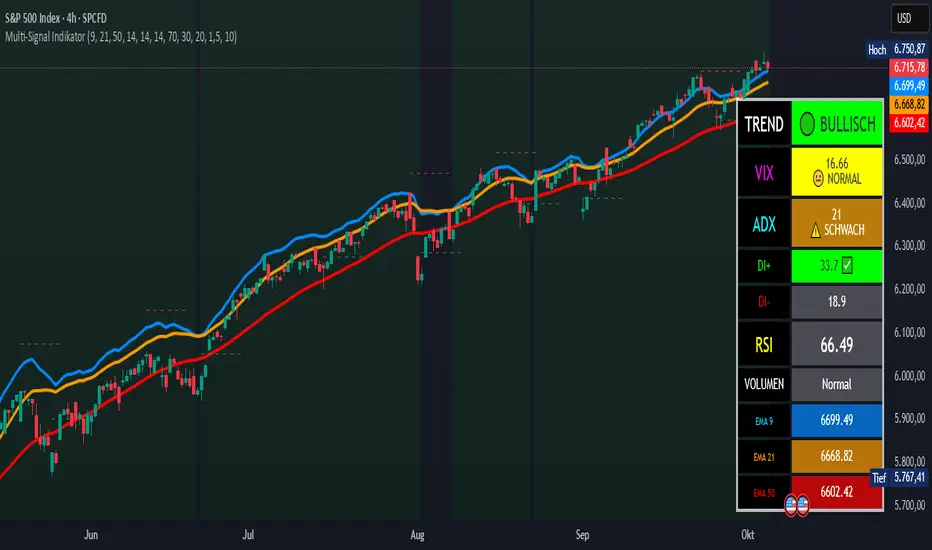
BTC 5-MA Multi Cross Strategy By Hardik Prajapati Ai TradelabThis strategy is built around the five most powerful and commonly used moving averages in crypto trading — 5, 20, 50, 100, and 200-period SMAs (Simple Moving Averages) — applied on a 1-hour Bitcoin chart.
Core Idea:
The strategy aims to identify strong bullish trends by confirming when the price action crosses above all key moving averages. This alignment of multiple MAs indicates momentum shift and helps filter out false breakouts.
⸻
⚙️ How It Works:
1. Calculates 5 Moving Averages:
• 5 MA → Short-term momentum (fastest signal)
• 20 MA → Near-term trend confirmation
• 50 MA → Mid-term trend filter
• 100 MA → Long-term trend foundation
• 200 MA → Macro-trend direction (strongest support/resistance)
2. Buy Condition (Entry):
• A Buy is triggered when:
• The price crosses above the 5 MA, and
• The closing price remains above all other MAs (20, 50, 100, 200)
This signals that momentum is aligned across all time horizons — a strong uptrend confirmation.
3. Sell Condition (Exit):
• The position is closed when price crosses below the 20 MA, showing weakness in short-term momentum.
4. Visual Signals:
• 🟢 BUY triangle below candles → Entry signal
• 🔴 SELL triangle above candles → Exit signal
• Colored MAs plotted for trend clarity.
⸻
📈 Recommended Usage:
• Chart: BTC/USDT
• Timeframe: 1 Hour
• Type: Trend-following crossover strategy
• Ideal for: Identifying major breakout moves and confirming trend reversals.
⸻
⚠️ Notes:
• This script is meant for educational and backtesting purposes only.
• Always apply additional confirmation tools (like RSI, Volume, or VIX-style filters) before live trading.
• Works best during trending markets; may produce whipsaws in sideways zones.

Flat Day PredictorAdvanced technical indicator that predicts low-volatility "flat" trading days using multi-factor analysis. Designed for day traders and scalpers who need to identify when markets are likely to trade sideways.
Key Features:
Real-time flat day probability calculation (0-100%)
8-factor scoring system combining volatility, volume, and momentum indicators
Visual table displaying all indicator values and overall signal strength
Color-coded alerts for high-probability flat day signals
Works on all timeframes, optimized for intraday trading
Indicators Analyzed:
VIX volatility levels
Bollinger Band width compression
RSI momentum neutrality
ATR trend declining
Volume below average
Daily range percentage
Price action patterns
Market regime detection
Signal Levels:
75%+ = VERY HIGH flat probability (Red alert)
62-74% = HIGH flat probability (Orange)
50-61% = MODERATE flat probability (Yellow)
Below 50% = Trending day likely (Green)
Usage:
Add to any chart and monitor the probability percentage. Higher scores indicate increased likelihood of sideways price action. Use for position sizing, strategy selection, and risk management during low-volatility periods.

Opening Range IndicatorComplete Trading Guide: Opening Range Breakout Strategy
What Are Opening Ranges?
Opening ranges capture the high and low prices during the first few minutes of market open. These levels often act as key support and resistance throughout the trading day because:
Heavy volume occurs at market open as overnight orders execute
Institutional activity is concentrated during opening minutes
Price discovery happens as market participants react to overnight news
Psychological levels are established that traders watch all day
Understanding the Three Timeframes
OR5 (5-Minute Range: 9:30-9:35 AM)
Most sensitive - captures immediate market reaction
Quick signals but higher false breakout rate
Best for scalping and momentum trading
Use for early entry when conviction is high
OR15 (15-Minute Range: 9:30-9:45 AM)
Balanced approach - most popular among day traders
Moderate sensitivity with better reliability
Good for swing trades lasting several hours
Primary timeframe for most strategies
OR30 (30-Minute Range: 9:30-10:00 AM)
Most reliable but slower signals
Lower false breakout rate
Best for position trades and trend following
Use when looking for major moves
Core Trading Strategies
Strategy 1: Basic Breakout
Setup:
Wait for price to break above OR15 high or below OR15 low
Enter on the breakout candle close
Stop loss: Opposite side of the range
Target: 2-3x the range size
Example:
OR15 range: $100.00 - $102.00 (Range = $2.00)
Long entry: Break above $102.00
Stop loss: $99.50 (below OR15 low)
Target: $104.00+ (2x range size)
Strategy 2: Multiple Confirmation
Setup:
Wait for OR5 break first (early signal)
Confirm with OR15 break in same direction
Enter on OR15 confirmation
Stop: Below OR30 if available, or OR15 opposite level
Why it works:
Multiple timeframe confirmation reduces false signals and increases probability of sustained moves.
Strategy 3: Failed Breakout Reversal
Setup:
Price breaks OR15 level but fails to hold
Wait for re-entry into the range
Enter reversal trade toward opposite OR level
Stop: Recent breakout high/low
Target: Opposite side of range + extension
Key insight: Failed breakouts often lead to strong moves in the opposite direction.
Advanced Techniques
Range Quality Assessment
High-Quality Ranges (Trade these):
Range size: 0.5% - 2% of stock price
Clean boundaries (not choppy)
Volume spike during range formation
Clear rejection at range levels
Low-Quality Ranges (Avoid these):
Very narrow ranges (<0.3% of stock price)
Extremely wide ranges (>3% of stock price)
Choppy, overlapping candles
Low volume during formation
Volume Confirmation
For Breakouts:
Look for volume spike (2x+ average) on breakout
Declining volume often signals false breakout
Rising volume during range formation shows interest
Market Context Filters
Best Conditions:
Trending market days (SPY/QQQ with clear direction)
Earnings reactions or news-driven moves
High-volume stocks with good liquidity
Volatility above average (VIX considerations)
Avoid Trading When:
Extremely low volume days
Major economic announcements pending
Holidays or half-days
Choppy, sideways market conditions
Risk Management Rules
Position Sizing
Conservative: Risk 0.5% of account per trade
Moderate: Risk 1% of account per trade
Aggressive: Risk 2% maximum per trade
Stop Loss Placement
Inside the range: Quick exit but higher stop-out rate
Outside opposite level: More room but larger risk
ATR-based: 1.5-2x Average True Range below entry
Profit Taking
Target 1: 1x range size (take 50% off)
Target 2: 2x range size (take 25% off)
Runner: Trail remaining 25% with moving stops
Specific Entry Techniques
Breakout Entry Methods
Method 1: Immediate Entry
Enter as soon as price closes above/below range
Fastest entry but highest false signal rate
Best for strong momentum situations
Method 2: Pullback Entry
Wait for breakout, then pullback to range level
Enter when price bounces off former resistance/support
Better risk/reward but may miss some moves
Method 3: Volume Confirmation
Wait for breakout + volume spike
Enter after volume confirmation candle
Reduces false signals significantly
Multiple Timeframe Entries
Aggressive: OR5 break → immediate entry
Conservative: OR5 + OR15 + OR30 all align → enter
Balanced: OR15 break with OR30 support → enter
Common Mistakes to Avoid
1. Trading Poor-Quality Ranges
❌ Don't trade ranges that are too narrow or too wide
✅ Focus on clean, well-defined ranges with good volume
2. Ignoring Volume
❌ Don't chase breakouts without volume confirmation
✅ Always check for volume spike on breakouts
3. Over-Trading
❌ Don't force trades when ranges are unclear
✅ Wait for high-probability setups only
4. Poor Risk Management
❌ Don't risk more than planned or use tight stops in volatile conditions
✅ Stick to predetermined risk levels
5. Fighting the Trend
❌ Don't fade breakouts in strongly trending markets
✅ Align trades with overall market direction
Daily Trading Routine
Pre-Market (8:00-9:30 AM)
Check overnight news and earnings
Review major indices (SPY, QQQ, IWM)
Identify potential opening range candidates
Set alerts for range breakouts
Market Open (9:30-10:00 AM)
Watch opening range formation
Note volume and price action quality
Mark key levels on charts
Prepare for breakout signals
Trading Session (10:00 AM - 4:00 PM)
Execute breakout strategies
Manage existing positions
Trail stops as profits develop
Look for additional setups
Post-Market Review
Analyze winning and losing trades
Review range quality vs. outcomes
Identify improvement areas
Prepare for next session
Best Stocks/ETFs for Opening Range Trading
Large Cap Stocks (Best for beginners):
AAPL, MSFT, GOOGL, AMZN, TSLA
High liquidity, predictable behavior
Good range formation most days
ETFs (Consistent patterns):
SPY, QQQ, IWM, XLF, XLE
Excellent liquidity
Clear range boundaries
Mid-Cap Growth (Advanced traders):
Stocks with good volume (1M+ shares daily)
Recent news catalysts
Clean technical patterns
Performance Optimization
Track These Metrics:
Win rate by range type (OR5 vs OR15 vs OR30)
Average R/R (risk vs reward ratio)
Best performing market conditions
Time of day performance
Continuous Improvement:
Keep detailed trade journal
Review failed breakouts for patterns
Adjust position sizing based on win rate
Refine entry timing based on backtesting
Final Tips for Success
Start small - Paper trade or use tiny positions initially
Focus on quality - Better to miss trades than take bad ones
Stay disciplined - Stick to your rules even during losing streaks
Adapt to conditions - What works in trending markets may fail in choppy conditions
Keep learning - Markets evolve, so should your approach
The opening range strategy is powerful because it captures natural market behavior, but like all strategies, it requires practice, discipline, and proper risk management to be profitable long-term.

IV Rank (tasty-style) — VIXFix / HV ProxyIV Rank (tasty-style) — VIXFix / HV Proxy
Overview
This indicator replicates tastytrade’s IV Rank calculation—but built entirely inside TradingView.
Because TradingView does not expose live option-chain implied volatility, the script lets you choose between two widely used price-based IV proxies:
VIXFix (Williams VIX Fix): a fast-reacting volatility estimate derived from price extremes.
HV(30): 30-day annualized historical volatility of daily log returns.
The goal is to approximate the “rich vs. cheap” option volatility environment that traders use to decide whether to sell or buy premium.
Formula
IV Rank answers the question: Where is current implied volatility relative to its own 1-year range?
𝐼
𝑉
𝑅
=
𝐼
𝑉
𝑐
𝑢
𝑟
𝑟
𝑒
𝑛
𝑡
−
𝐼
𝑉
1
𝑦
𝐿
𝑜
𝑤
𝐼
𝑉
1
𝑦
𝐻
𝑖
𝑔
ℎ
−
𝐼
𝑉
1
𝑦
𝐿
𝑜
𝑤
×
100
IVR=
IV
1yHigh
−IV
1yLow
IV
current
−IV
1yLow
×100
IVcurrent: Current value of the chosen IV proxy.
IV1yHigh/Low: Highest and lowest proxy values over the user-defined lookback (default 252 trading days ≈ 1 year).
IVR = 0 → Current IV equals its 1-year low
IVR = 100 → Current IV equals its 1-year high
IVR ≈ 50 → Current IV sits mid-range
How to Use
High IV Rank (≥50–60%)
Options are relatively expensive → short-premium strategies (credit spreads, iron condors, straddles) may be more attractive.
Low IV Rank (≤20%)
Options are relatively cheap → long-premium strategies (debit spreads, calendars, diagonals) may offer better risk/reward.
Combine with your own analysis, liquidity checks, and risk management.
Inputs & Customization
IV Source: Choose “VIXFix” or “HV(30)” as the volatility proxy.
IVR Lookback: Rolling window for 1-year high/low (default 252 trading days).
VIXFix Parameters: Length and stdev multiplier to fine-tune sensitivity.
Info Label: Optional on-chart label displays current IV proxy, 1-year high/low, and IV Rank.
Alerts: Optional alerts when IVR crosses 50, falls below 20, or rises above 80.
Notes & Limitations
This indicator does not pull real option-chain IV.
It provides a close structural analogue to tastytrade’s IV Rank using price-derived proxies for markets where options data is not directly available.
For live option IV, use broker platforms or third-party data feeds alongside this script.
Tags: IV Rank, Implied Volatility, Tastytrade, VIXFix, Historical Volatility, Options, Premium Selling, Debit Spreads, Market Volatility
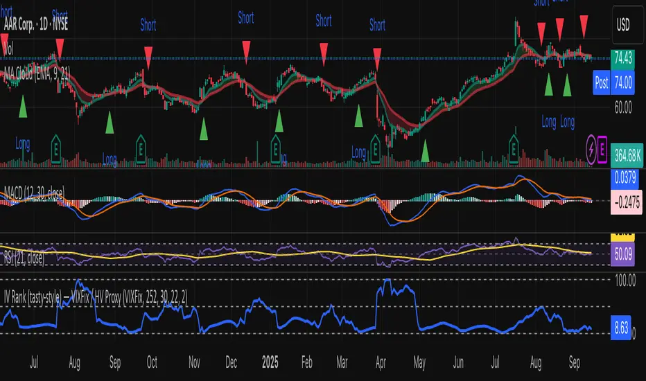
B3 – VIX + Breadth + SR + Projeção 14dA comprehensive technical analysis tool that combines volatility proxies (HV, ATR, BB Width, composite VolIndex), market breadth (internal and multi-timeframe), pivot-based support/resistance with strength and confluence, and a 14-day linear regression projection with confidence bands. Designed to provide a holistic view of trend, risk, and key price levels for swing and medium-term trading decisions.

BTC Macro Composite Global liquidity Index -OffsetThis indicator is based on the thesis that Bitcoin price movements are heavily influenced by macro liquidity trends. It calculates a weighted composite index based on the following components:
• Global Liquidity (41%): Sum of central bank balance sheets (Fed , ECB , BoJ , and PBoC ), adjusted to USD.
• Investor Risk Appetite (22%): Derived from the Copper/Gold ratio, inverse VIX (as a risk-on signal), and the spread between High Yield and Investment Grade bonds (HY vs IG OAS).
• Gold Sensitivity (15–20%): Combines the XAUUSD price with BTC/Gold ratio to reflect the historical influence of gold on Bitcoin pricing.
Each component is normalized and then offset forward by 90 days to attempt predictive alignment with Bitcoin’s price.
The goal is to identify macro inflection points with high predictive value for BTC. It is not a trading signal generator but rather a macro trend context indicator.
❗ Important: This script should be used with caution. It does not account for geopolitical shocks, regulatory events, or internal BTC market structure (e.g., miner behavior, on-chain metrics).
💡 How to use:
• Use on the 1D timeframe.
• Look for divergences between BTC price and the macro index.
• Apply in confluence with other technical or fundamental frameworks.
🔍 Originality:
While similar components exist in macro dashboards, this script combines them uniquely using time-forward offsets and custom weighting specifically tailored for BTC behavior.
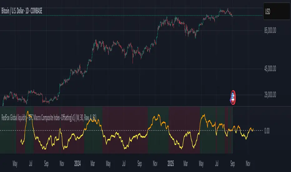
Overnight Gap Dominance Indicator (OGDI)The Overnight Gap Dominance Indicator (OGDI) measures the relative volatility of overnight price gaps versus intraday price movements for a given security, such as SPY or SPX. It uses a rolling standard deviation of absolute overnight percentage changes divided by the standard deviation of absolute intraday percentage changes over a customizable window. This helps traders identify periods where overnight gaps predominate, suggesting potential opportunities for strategies leveraging extended market moves.
Instructions
A
pply the indicator to your TradingView chart for the desired security (e.g., SPY or SPX).
Adjust the "Rolling Window" input to set the lookback period (default: 60 bars).
Modify the "1DTE Threshold" and "2DTE+ Threshold" inputs to tailor the levels at which you switch from 0DTE to 1DTE or multi-DTE strategies (default: 0.5 and 0.6).
Observe the OGDI line: values above the 1DTE threshold suggest favoring 1DTE strategies, while values above the 2DTE+ threshold indicate multi-DTE strategies may be more effective.
Use in conjunction with low VIX environments and uptrend legs for optimal results.
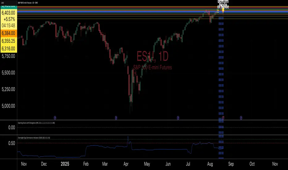
Information-Geometric Market DynamicsInformation-Geometric Market Dynamics
The Information Field: A Geometric Approach to Market Dynamics
By: DskyzInvestments
Foreword: Beyond the Shadows on the Wall
If you have traded for any length of time, you know " the feeling ." It is the frustration of a perfect setup that fails, the whipsaw that stops you out just before the real move, the nagging sense that the chart is telling you only half the story. For decades, technical analysis has relied on interpreting the shadows—the patterns left behind by price. We draw lines on these shadows, apply indicators to them, and hope they reveal the future.
But what if we could stop looking at the shadows and, instead, analyze the object casting them?
This script introduces a new paradigm for market analysis: Information-Geometric Market Dynamics (IGMD) . The core premise of IGMD is that the price chart is merely a one-dimensional projection of a much richer, higher-dimensional reality—an " information field " generated by the collective actions and beliefs of all market participants.
This is not just another collection of indicators. It is a unified framework for measuring the geometry of the market's information field—its memory, its complexity, its uncertainty, its causal flows—and making high-probability decisions based on that deeper reality. By fusing advanced mathematical and informational concepts, IGMD provides a multi-faceted lens through which to view market behavior, moving beyond simple price action into the very structure of market information itself.
Prepare to move beyond the flatland of the price chart. Welcome to the information field.
The IGMD Framework: A Multi-Kernel Approach
What is a Kernel? The Heart of Transformation
In mathematics and data science, a kernel is a powerful and elegant concept. At its core, a kernel is a function that takes complex, often inscrutable data and transforms it into a more useful format. Think of it as a specialized lens or a mathematical "probe." You cannot directly measure abstract concepts like "market memory" or "trend quality" by looking at a price number. First, you must process the raw price data through a specific mathematical machine—a kernel—that is designed to output a measurement of that specific property. Kernels operate by performing a sort of "similarity test," projecting data into a higher-dimensional space where hidden patterns and relationships become visible and measurable.
Why do creators use them? We use kernels to extract features —meaningful pieces of information—that are not explicitly present in the raw data. They are the essential tools for moving beyond surface-level analysis into the very DNA of market behavior. A simple moving average can tell you the average price; a suite of well-chosen kernels can tell you about the character of the price action itself.
The Alchemist's Challenge: The Art of Fusion
Using a single kernel is a challenge. Using five distinct, computationally demanding mathematical engines in unison is an immense undertaking. The true difficulty—and artistry—lies not just in using one kernel, but in fusing the outputs of many . Each kernel provides a different perspective, and they can often give conflicting signals. One kernel might detect a strong trend, while another signals rising chaos and uncertainty. The IGMD script's greatest strength is its ability to act as this alchemist, synthesizing these disparate viewpoints through a weighted fusion process to produce a single, coherent picture of the market's state. It required countless hours of testing and calibration to balance the influence of these five distinct analytical engines so they work in harmony rather than cacophony.
The Five Kernels of Market Dynamics
The IGMD script is built upon a foundation of five distinct kernels, each chosen to probe a unique and critical dimension of the market's information field.
1. The Wavelet Kernel (The "Microscope")
What it is: The Wavelet Kernel is a signal processing function designed to decompose a signal into different frequency scales. Unlike a Fourier Transform that analyzes the entire signal at once, the wavelet slides across the data, providing information about both what frequencies are present and when they occurred.
The Kernels I Use:
Haar Kernel: The simplest wavelet, a square-wave shape defined by the coefficients . It excels at detecting sharp, sudden changes.
Daubechies 2 (db2) Kernel: A more complex and smoother wavelet shape that provides a better balance for analyzing the nuanced ebb and flow of typical market trends.
How it Works in the Script: This kernel is applied iteratively. It first separates the finest "noise" (detail d1) from the first level of trend (approximation a1). It then takes the trend a1 and repeats the process, extracting the next level of cycle (d2) and trend (a2), and so on. This hierarchical decomposition allows us to separate short-term noise from the long-term market "thesis."
2. The Hurst Exponent Kernel (The "Memory Gauge")
What it is: The Hurst Exponent is derived from a statistical analysis kernel that measures the "long-term memory" or persistence of a time series. It is the definitive measure of whether a series is trending (H > 0.5), mean-reverting (H < 0.5), or random (H = 0.5).
How it Works in the Script: The script employs a method based on Rescaled Range (R/S) analysis. It calculates the average range of price movements over increasingly larger time lags (m1, m2, m4, m8...). The slope of the line plotting log(range) vs. log(lag) is the Hurst Exponent. Applying this complex statistical analysis not to the raw price, but to the clean, wavelet-decomposed trend lines, is a key innovation of IGMD.
3. The Fractal Dimension Kernel (The "Complexity Compass")
What it is: This kernel measures the geometric complexity or "jaggedness" of a price path, based on the principles of fractal geometry. A straight line has a dimension of 1; a chaotic, space-filling line approaches a dimension of 2.
How it Works in the Script: We use a version based on Ehlers' Fractal Dimension Index (FDI). It calculates the rate of price change over a full lookback period (N3) and compares it to the sum of the rates of change over the two halves of that period (N1 + N2). The formula d = (log(N1 + N2) - log(N3)) / log(2) quantifies how much "longer" and more convoluted the price path was than a simple straight line. This kernel is our primary filter for tradeable (low complexity) vs. untradeable (high complexity) conditions.
4. The Shannon Entropy Kernel (The "Uncertainty Meter")
What it is: This kernel comes from Information Theory and provides the purest mathematical measure of information, surprise, or uncertainty within a system. It is not a measure of volatility; a market moving predictably up by 10 points every bar has high volatility but zero entropy .
How it Works in the Script: The script normalizes price returns by the ATR, categorizes them into a discrete number of "bins" over a lookback window, and forms a probability distribution. The Shannon Entropy H = -Σ(p_i * log(p_i)) is calculated from this distribution. A low H means returns are predictable. A high H means returns are chaotic. This kernel is our ultimate gauge of market conviction.
5. The Transfer Entropy Kernel (The "Causality Probe")
What it is: This is by far the most advanced and computationally intensive kernel in the script. Transfer Entropy is a non-parametric measure of directed information flow between two time series. It moves beyond correlation to ask: "Does knowing the past of Volume genuinely reduce our uncertainty about the future of Price?"
How it Works in the Script: To make this work, the script discretizes both price returns and the chosen "driver" (e.g., OBV) into three states: "up," "down," or "neutral." It then builds complex conditional probability tables to measure the flow of information in both directions. The Net Transfer Entropy (TE Driver→Price minus TE Price→Driver) gives us a direct measure of causality . A positive score means the driver is leading price, confirming the validity of the move. This is a profound leap beyond traditional indicator analysis.
Chapter 3: Fusion & Interpretation - The Field Score & Dashboard
Each kernel is a specialist providing a piece of the puzzle. The Field Score is where they are fused into a single, comprehensive reading. It's a weighted sum of the normalized scores from all five kernels, producing a single number from -1 (maximum bearish information field) to +1 (maximum bullish information field). This is the ultimate "at-a-glance" metric for the market's net state, and it is interpreted through the dashboard.
The Dashboard: Your Mission Control
Field Score & Regime: The master metric and its plain-English interpretation ("Uptrend Field", "Downtrend Field", "Transitional").
Kernel Readouts (Wave Align, H(w), FDI, etc.): The live scores of each individual kernel. This allows you to see why the Field Score is what it is. A high Field Score with all components in agreement (all green or red) is a state of High Coherence and represents a high-quality setup.
Market Context: Standard metrics like RSI and Volume for additional confluence.
Signals: The raw and adjusted confluence counts and the final, calculated probability scores for potential long and short entries.
Pattern: Shows the dominant candlestick pattern detected within the currently forming APEX range box and its calculated confidence percentage.
Chapter 4: Mastering the Controls - The Inputs Menu
Every parameter is a lever to fine-tune the IGMD engine.
📊 Wavelet Transform: Kernel ( Haar for sharp moves, db2 for smooth trends) and Scales (depth of analysis) let you tune the script's core microscope to your asset's personality.
📈 Hurst Exponent: The Window determines if you're assessing short-term or long-term market memory.
🔍 Fractal Dimension & ⚡ Entropy Volatility: Adjust the lookback windows to make these kernels more or less sensitive to recent price action. Always keep "Normalize by ATR" enabled for Entropy for consistent results.
🔄 Transfer Entropy: Driver lets you choose what causal force to measure (e.g., OBV, Volume, or even an external symbol like VIX). The throttle setting is a crucial performance tool, allowing you to balance precision with script speed.
⚡ Field Fusion • Weights: This is where you can customize the model's "brain." Increase the weights for the kernels that best align with your trading philosophy (e.g., w_hurst for trend followers, w_fdi for chop avoiders).
📊 Signal Engine: Mode offers presets from Conservative to Aggressive . Min Confluence sets your evidence threshold. Dynamic Confluence is a powerful feature that automatically adapts this threshold to the market regime.
🎨 Visuals & 📏 Support/Resistance: These inputs give you full control over the chart's appearance, allowing you to toggle every visual element for a setup that is as clean or as data-rich as you desire.
Chapter 5: Reading the Battlefield - On-Chart Visuals
Pattern Boxes (The Large Rectangles): These are not simple range boxes. They appear when the Field Score crosses a significance threshold, signaling a potential ignition point.
Color: The color reflects the dominant candlestick pattern that has occurred within that box's duration (e.g., green for Bull Engulf).
Label: Displays the dominant pattern, its duration in bars, and a calculated Confidence % based on field strength and pattern clarity.
Bar Pattern Boxes (The Small Boxes): If enabled, these highlight individual, significant candlestick patterns ( BE for Bull Engulf, H for Hammer) on a bar-by-bar basis.
Signal Markers (▲ and ▼): These appear only when the Signal Engine's criteria are all met. The number is the calculated Probability Score .
RR Rails (Dashed Lines): When a signal appears, these lines automatically plot the Entry, Stop Loss (based on ATR), and two Take Profit targets (based on Risk/Reward ratios). They dynamically break and disappear as price touches each level.
Support & Resistance Lines: Plots of the highest high ( Resistance ) and lowest low ( Support ) over a lookback, providing key structural levels.
Chapter 6: Development Philosophy & A Final Word
One single question: " What is the market really doing? " It represents a triumph of complexity, blending concepts from signal processing, chaos theory, and information theory into a cohesive framework. It is offered for educational and analytical purposes and does not constitute financial advice. Its goal is to elevate your analysis from interpreting flat shadows to measuring the rich, geometric reality of the market's information field.
As the great mathematician Benoit Mandelbrot , father of fractal geometry, noted:
"Clouds are not spheres, mountains are not cones, coastlines are not circles, and bark is not smooth, nor does lightning travel in a straight line."
Neither does the market. IGMD is a tool designed to navigate that beautiful, complex, and fractal reality.
— Dskyz, Trade with insight. Trade with anticipation.

US Macro Cycle (Z-Score Model)US Macro Cycle (Z-Score Model)
This indicator tracks the US economic cycle in real time using a weighted composite of seven macro and market-based indicators, each converted into a rolling Z-score for comparability. The model identifies the current phase of the cycle — Expansion, Peak, Contraction, or Recovery — and suggests sector tilts based on historical performance in each phase.
Core Components:
Yield Curve (10y–2y): Positive & steepening = growth; inverted = slowdown risk.
Credit Spreads (HYG/LQD): Tightening = risk-on; widening = risk-off.
Sector Leadership (Cyclicals vs. Defensives): Measures market leadership regime.
Copper/Gold Ratio: Higher copper = growth signal; higher gold = defensive.
SPY vs. 200-day MA: Equity trend strength.
SPY/IEF Ratio: Stocks vs. bonds relative strength.
VIX (Inverted): Low/falling volatility = supportive; high/rising = risk-off.
Methodology:
Each series is transformed into a rolling Z-score over the selected lookback period (optionally using median/MAD for robustness and winsorization to clip outliers).
Z-scores are combined using user-defined weights and normalized.
The smoothed composite is compared against phase thresholds to classify the macro environment.
Features:
Customizable Weights: Emphasize the indicators most relevant to your strategy.
Adjustable Thresholds: Fine-tune cycle phase definitions.
Background Coloring: Visual cue for the current phase.
Summary Table: Displays composite Z, confidence %, and individual Z-scores.
Alerts: Trigger when the phase changes, with details on the composite score and recommended tilt.
Use Cases:
Align sector rotation or relative strength strategies with the macro backdrop.
Identify favorable or defensive phases for tactical allocation.
Monitor macro turning points to manage portfolio risk.
It's doesn't fill nan gaps so there is quite a bit of zeroes, non-repainting.