Z-Score Trend Monitor [EdgeTerminal]The Z-Score Trend Monitor measures how far the short-term moving average deviates from the long-term moving average using the spread difference of the two — in standardized units. It’s designed to detect overextension, momentum exhaustion, and potential mean-reversion points by converting the spread between two moving averages into a normalized Z-score and tracking its change and direction over time.
The idea behind this is to catch the changes in the direction of a trend earlier than the usual and lagging moving average lines, allowing you to react faster.
The math behind the indicator itself is very simple. We take the simple moving average of the spread between a long term and short term moving average, and divide it by the difference between the spread and spread mean.
This results in a relatively accurate and early acting trend detector that can easily identify overbought and oversold levels in any timeframe. From our own testing, we recommend using this indicator as a trend confirmation tool.
How to Use It:
Keep an eye on the Z-Score or the blue line. When it goes over 2, it indicates an overbought or near top level, and when it goes below -2, it indicates an oversold or near bottom.
When Z-Score returns to zero or grey line, it suggests mean reversion is in progress.
You can also change the Z-Score criteria from 2 and -2 in the settings to any number you’d like for tighter or wider levels.
For scalping and fast trading setups, we recommend shorter SMAs, such as 5 and 20, and for longer trading setups such as swing trades, we recommend 20 and 100.
Settings:
Short SMA: Lookback period of short term simple moving average for the lower side of the SMA spread.
Short Term Weight: Additional weight or multiplier to suppress the short term SMA calculation. This is used to refine the SMA calculation for more granular and edge cases when needed, usually left at 1, meaning it will take the entire given value in the short SMA field.
Long SMA: Lookback period of long term simple moving average for the upper side of the SMA spread.
Long Term Weight: Additional weight or multiplier to suppress the long term SMA calculation. This is used to refine the long SMA calculation for more granular and edge cases when needed, usually left at 1, meaning it will take the entire given value in the long SMA field.
Z-Score Threshold: The threshold for upper (oversold) and lower (overbought) levels. This can also be set individually from the style page.
Z-Score Lookback Window: The lookback period to calculate spread mean and spread standard deviation
Cerca negli script per "如何用wind搜索股票的发行价和份数"

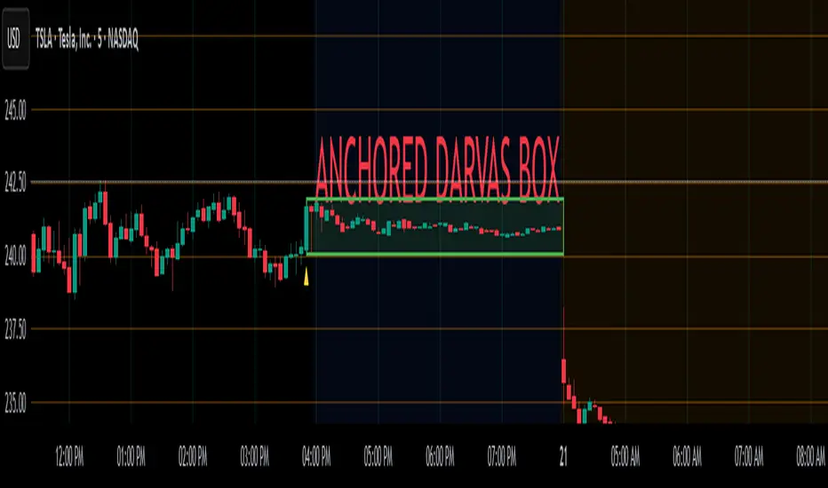
Anchored Darvas Box## ANCHORED DARVAS BOX
---
### OVERVIEW
**Anchored Darvas Box** lets you drop a single timestamp on your chart and build a Darvas-style consolidation zone forward from that exact candle. The indicator freezes the first user-defined number of bars to establish the range, verifies that price respects that range for another user-defined number of bars, then waits for the first decisive breakout. The resulting rectangle captures every tick of the accumulation phase and the exact moment of expansion—no manual drawing, complete timestamp precision.
---
### HISTORICAL BACKGROUND
Nicolas Darvas’s 1950s box theory tracked institutional accumulation by hand-drawing rectangles around tight price ranges. A trade was triggered only when price escaped the rectangle.
The anchored version preserves Darvas’s logic but pins the entire sequence to a user-chosen candle: perfect for analysing a market open, an earnings release, FOMC minute, or any other catalytic bar.
---
### ALGORITHM DETAIL
1. **ANCHOR BAR**
*You provide a timestamp via the settings panel.* The script waits until the chart reaches that bar and records its index as **startBar**.
2. **RANGE DEFINITION — BARS 1-7**
• `rangeHigh` = highest high of bars 1-7 plus optional tolerance.
• `rangeLow` = lowest low of bars 1-7 minus optional tolerance.
3. **RANGE VALIDATION — BARS 8-14**
• Price must stay inside ` `.
• Any violation aborts the test; no box is created.
4. **ARMED STATE**
• If bars 8-14 hold the range, two live guide-lines appear:
– **Green** at `rangeHigh`
– **Red** at `rangeLow`
• The script is now “armed,” waiting indefinitely for the first true breakout.
5. **BREAKOUT & BOX CREATION**
• **Up breakout** =`high > rangeHigh` → rectangle drawn in **green**.
• **Down breakout**=`low < rangeLow` → rectangle drawn in **red**.
• Box extends from **startBar** to the breakout bar and never updates again.
• Optional labels print the dollar and percentage height of the box at its left edge.
6. **OPTIONAL COOLDOWN**
• After the box is painted the script can stay silent for a user-defined number of bars, letting you study the fallout without another range immediately arming on top of it.
---
### INPUT PARAMETERS
• **ANCHOR TIME** – Precise yyyy-mm-dd HH:MM:SS that seeds the sequence.
• **BARS TO DEFINE RANGE** – Default 7; affects both definition and validation windows.
• **OPTIONAL TOLERANCE** – Absolute price buffer to ignore micro-wicks.
• **COOLDOWN BARS AFTER BREAKOUT** – Pause length before the indicator is allowed to re-anchor (set to zero to disable).
• **SHOW BOX DISTANCE LABELS** – Toggle to print Δ\$ and Δ% on every completed box.
---
### USER WORKFLOW
1. Add the indicator, open settings, and set **ANCHOR TIME** to the candle you care about (e.g., “2025-04-23 09:30:00” for NYSE open).
2. Watch live as the script:
– Paints the seven-bar range.
– Draws validation lines.
– Locks in the box on breakout.
3. Use the box boundaries as structural stops, targets, or context for further trades.
---
### PRACTICAL APPLICATIONS
• **OPENING RANGE BREAKOUTS** – Anchor at the first second of the session; capture the initial 7-bar range and trade the first clean break.
• **EVENT STUDIES** – Anchor at a news candle to measure immediate post-event volatility.
• **VOLUME PROFILE FUSION** – Combine the anchored box with VPVR to see if the breakout occurs at a high-volume node or a low-liquidity pocket.
• **RISK DISCIPLINE** – Stop-loss can sit just inside the opposite edge of the anchored range, enforcing objective risk.
---
### ADVANCED CUSTOMISATION IDEAS
• **MULTIPLE ANCHORS** – Clone the indicator and anchor several boxes (e.g., London open, New York open).
• **DYNAMIC WINDOW** – Switch the 7-bar fixed length to a volatility-scaled length (ATR percentile).
• **STRATEGY WRAPPER** – Turn the indicator into a `strategy{}` script and back-test anchored boxes on decades of data.
---
### FINAL THOUGHTS
Anchored Darvas Boxes give you Darvas’s timeless range-break methodology anchored to any candle of interest—perfect for dissecting openings, economic releases, or your own bespoke “important” bars with laboratory precision.
Express Generator StrategyExpress Generator Strategy
Pine Script™ v6
The Express Generator Strategy is an algorithmic trading system that harnesses confluence from multiple technical indicators to optimize trade entries and dynamic risk management. Developed in Pine Script v6, it is designed to operate within a user-defined backtesting period—ensuring that trades are executed only during chosen historical windows for targeted analysis.
How It Works:
- Entry Conditions:
The strategy relies on a dual confirmation approach:- A moving average crossover system where a fast (default 9-period SMA) crossing above or below a slower (default 21-period SMA) average signals a potential trend reversal.
- MACD confirmation; trades are only initiated when the MACD line crosses its signal line in the direction of the moving average signal.
- An RSI filter refines these signals by preventing entries when the market might be overextended—ensuring that long entries only occur when the RSI is below an overbought level (default 70) and short entries when above an oversold level (default 30).
- Risk Management & Dynamic Position Sizing:
The strategy takes a calculated approach to risk by enabling the adjustment of position sizes using:- A pre-defined percentage of equity risk per trade (default 1%, adjustable between 0.5% to 3%).
- A stop-loss set in pips (default 100 pips, with customizable ranges), which is then adjusted by market volatility measured through the ATR.
- Trailing stops (default 50 pips) to help protect profits as the market moves favorably.
This combination of volatility-adjusted risk and equity-based position sizing aims to harmonize trade exposure with prevailing market conditions.
- Backtest Period Flexibility:
Users can define the start and end dates for backtesting (e.g., January 1, 2020 to December 31, 2025). This ensures that the strategy only opens trades within the intended analysis window. Moreover, if the strategy is still holding a position outside this period, it automatically closes all trades to prevent unwanted exposure.
- Visual Insights:
For clarity, the strategy plots the fast (blue) and slow (red) moving averages directly on the chart, allowing for visual confirmation of crossovers and trend shifts.
By integrating multiple technical indicators with robust risk management and adaptable position sizing, the Express Generator Strategy provides a comprehensive framework for capturing trending moves while prudently managing downside risk. It’s ideally suited for traders looking to combine systematic entries with a disciplined and dynamic risk approach.

Volume and Volatility Ratio Indicator-WODI该指标名为“交易量与波动率比例指标-WODI”,主要基于交易量和价格波动率构造一个复合指数,帮助识别市场内可能存在的异常或转折信号。具体实现如下:
用户自定义参数
用户可以设置交易量均线长度(vol_length)、指数的短期与长期均线长度(index_short_length、index_long_length)、均线敏感度(index_magnification)、阈值放大因子(index_threshold_magnification)以及检测K线形态的区间(lookback_bars)。这些参数为后续计算提供了灵活性,允许用户根据不同市场环境自定义指标的敏感度和响应速度。
交易量均线与百分比计算
首先通过 ta.sma 计算指定长度的交易量简单均线(vol_ma)。
接下来,将当前交易量与均线进行比较,计算出当前交易量占均线的百分比(vol_percent),这反映了短期内交易量的相对活跃程度。
波动率的衡量
使用当前K线的最高价和最低价计算振幅,再除以收盘价乘以100得到波动率(volatility),从而反映市场价格波动的幅度。
构建交易量/波动率指数
将交易量百分比与波动率相乘,形成了“交易量/波动率指数”(volatility_index)。该指数能够同时反映市场的交易活跃度和价格波动性,两者的联合作用帮助捕捉市场的“热度”。
计算指标均线与阈值
对交易量/波动率指数分别计算短期均线(index_short_ma)和长期均线(index_long_ma),并通过乘以一个敏感度参数(index_magnification)进行调整。
同时,依据长期均线计算一个阈值(index_threshold),起到过滤噪音的作用。当指数突破该阈值时,可能预示着市场的重要变化。
K线形态与反转模式检测
通过遍历最近几根K线(由lookback_bars控制),指标会检测是否符合一系列预定条件(涉及交易量、价格振幅、K线形态等),以判断是否存在反转模式。若符合条件,则标记为反转模式,从而为潜在的转折点提供提示。
图表展示
最终在独立窗口中绘制多个元素:
指数短均线与长均线:经过敏感度调整后显示,用于分析指数趋势。
交易量/波动率指数:采用阶梯线风格绘制,直观展示指数变化。
阈值线:作为参考水平,便于判断指数是否突破常规范围。
交易量柱状图:当当前交易量高于均线时,通过不同颜色显示;当检测到反转模式时,颜色会进一步强化,帮助用户迅速识别潜在信号。
English Description
This indicator, titled “Volume and Volatility Ratio Indicator - WODI”, is designed to construct a composite index based on trading volume and price volatility, aiding in the identification of abnormal market conditions or potential reversal signals. Its functionality is broken down as follows:
User-Defined Parameters
The indicator allows users to set parameters such as the moving average length for volume (vol_length), the short and long moving average lengths for the index (index_short_length and index_long_length), a sensitivity multiplier (index_magnification), a threshold magnification factor (index_threshold_magnification), and the number of bars for pattern detection (lookback_bars). These parameters provide flexibility to adjust the sensitivity and responsiveness of the indicator based on different market conditions.
Volume Moving Average and Percentage Calculation
A simple moving average (SMA) of volume is computed over the specified length (vol_ma) using the ta.sma function.
The current volume is then compared to its moving average to calculate the volume percentage (vol_percent), reflecting the relative trading intensity in the short term.
Measuring Volatility
Volatility is calculated based on the current bar’s high and low prices, normalized by the closing price and multiplied by 100, which provides a measure of the market’s price fluctuation magnitude.
Constructing the Volume/Volatility Index
The index (volatility_index) is derived by multiplying the volume percentage by the calculated volatility. This composite metric reflects both market activity and price movement, effectively capturing the overall “heat” of the market.
Calculating the Index Moving Averages and Threshold
Two moving averages for the volatility_index are computed: one short-term (index_short_ma) and one long-term (index_long_ma). These are then adjusted by the sensitivity multiplier (index_magnification).
A threshold level (index_threshold) is calculated based on the long-term moving average multiplied by the threshold magnification factor, serving to filter out market noise. When the index exceeds this threshold, it may signal significant market shifts.
Detection of Reversal Patterns
The indicator iterates through the recent bars (as determined by lookback_bars) to check whether a set of predetermined conditions (involving trends in the volatility_index, volume comparisons, price closes, and K-line patterns) are met. If these conditions are satisfied, it flags a reversal pattern, which may serve as a warning for a potential market turnaround.
Visualization on the Chart
The final display includes several elements plotted in a separate indicator window:
The short-term and long-term moving averages of the index (after sensitivity adjustment) which help visualize the trend of the composite index.
The volatility index itself is drawn using a step-line style for clarity.
A threshold line is plotted to provide a reference level against which index movements can be compared.
A volume histogram is also displayed, where bars are colored differently when the current volume exceeds the moving average; the color is further enhanced if a reversal pattern is detected, making it easy for users to quickly spot potential signals.
MACD Crossover Breakout Rays with VWAP & Breakout ConfirmationOverview
This script is designed to highlight potential strong breakout moves by combining MACD crossovers, VWAP confirmation, and price action breakouts. It helps traders identify momentum shifts and filter high-probability trade setups.
How It Works
1. MACD Crossover Detection
- The script detects bullish crossovers (MACD line crossing above the signal line) and bearish crossovers (MACD line crossing below the signal line).
- A horizontal ray is drawn at the high (bullish) or low (bearish) of the crossover candle.
2. Multi-Timeframe MACD Confirmation
- A secondary MACD crossover is checked on a lower timeframe (default: 5 minutes) to confirm the strength of the move.
- The script ensures alignment between the primary and lower timeframe MACD crossovers before signaling a strong move.
3. VWAP Confirmation
- A bullish breakout is valid only if the price is above the VWAP.
- A bearish breakout is valid only if the price is below the VWAP.
4. Breakout Validation
- The script waits for price action confirmation—a breakout is only valid when a candle closes above (bullish) or below (bearish) the horizontal ray.
- Once confirmed, the ray color changes to blue to signal a strong move.
5. Label Alerts for Strong Moves
- When all conditions align, the script prints "STRONG 💪 MOVE" above or below the breakout candle.
- The previous label is automatically removed to keep the chart clean.
Customization Options
- MACD Settings: Adjust fast/slow lengths and signal smoothing.
- Lower Timeframe Confirmation: Choose a different timeframe for multi-timeframe MACD validation.
- VWAP Filtering: Ensure breakouts align with volume-weighted trends.
- Ray Length & Colors: Customize the horizontal ray length, width, and colors.
- Breakout Confirmation Window: Adjust how many bars to check for MACD alignment.
Best Use Cases
✅ Identifying high-probability breakouts with trend confirmation.
✅ Filtering out false signals by requiring multi-timeframe agreement.
✅ Helping traders stay in momentum-driven moves with strong confirmation.
⚠ Note: This script is for educational purposes only and does not constitute financial advice. Always conduct your own analysis before making trading decisions.

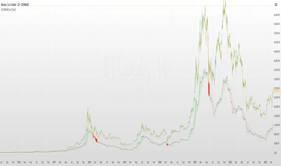
iD EMARSI on ChartSCRIPT OVERVIEW
The EMARSI indicator is an advanced technical analysis tool that maps RSI values directly onto price charts. With adaptive scaling capabilities, it provides a unique visualization of momentum that flows naturally with price action, making it particularly valuable for FOREX and low-priced securities trading.
KEY FEATURES
1 PRICE MAPPED RSI VISUALIZATION
Unlike traditional RSI that displays in a separate window, EMARSI plots the RSI directly on the price chart, creating a flowing line that identifies momentum shifts within the context of price action:
// Map RSI to price chart with better scaling
mappedRsi = useAdaptiveScaling ?
median + ((rsi - 50) / 50 * (pQH - pQL) / 2 * math.min(1.0, 1/scalingFactor)) :
down == pQL ? pQH : up == pQL ? pQL : median - (median / (1 + up / down))
2 ADAPTIVE SCALING SYSTEM
The script features an intelligent scaling system that automatically adjusts to different market conditions and price levels:
// Calculate adaptive scaling factor based on selected method
scalingFactor = if scalingMethod == "ATR-Based"
math.min(maxScalingFactor, math.max(1.0, minTickSize / (atrValue/avgPrice)))
else if scalingMethod == "Price-Based"
math.min(maxScalingFactor, math.max(1.0, math.sqrt(100 / math.max(avgPrice, 0.01))))
else // Volume-Based
math.min(maxScalingFactor, math.max(1.0, math.sqrt(1000000 / math.max(volume, 100))))
3 MODIFIED RSI CALCULATION
EMARSI uses a specially formulated RSI calculation that works with an adaptive base value to maintain consistency across different price ranges:
// Adaptive RSI Base based on price levels to improve flow
adaptiveRsiBase = useAdaptiveScaling ? rsiBase * scalingFactor : rsiBase
// Calculate RSI components with adaptivity
up = ta.rma(math.max(ta.change(rsiSourceInput), adaptiveRsiBase), emaSlowLength)
down = ta.rma(-math.min(ta.change(rsiSourceInput), adaptiveRsiBase), rsiLengthInput)
// Improved RSI calculation with value constraint
rsi = down == 0 ? 100 : up == 0 ? 0 : 100 - (100 / (1 + up / down))
4 MOVING AVERAGE CROSSOVER SYSTEM
The indicator creates a smooth moving average of the RSI line, enabling a crossover system that generates trading signals:
// Calculate MA of mapped RSI
rsiMA = ma(mappedRsi, emaSlowLength, maTypeInput)
// Strategy entries
if ta.crossover(mappedRsi, rsiMA)
strategy.entry("RSI Long", strategy.long)
if ta.crossunder(mappedRsi, rsiMA)
strategy.entry("RSI Short", strategy.short)
5 VISUAL REFERENCE FRAMEWORK
The script includes visual guides that help interpret the RSI movement within the context of recent price action:
// Calculate pivot high and low
pQH = ta.highest(high, hlLen)
pQL = ta.lowest(low, hlLen)
median = (pQH + pQL) / 2
// Plotting
plot(pQH, "Pivot High", color=color.rgb(82, 228, 102, 90))
plot(pQL, "Pivot Low", color=color.rgb(231, 65, 65, 90))
med = plot(median, style=plot.style_steplinebr, linewidth=1, color=color.rgb(238, 101, 59, 90))
6 DYNAMIC COLOR SYSTEM
The indicator uses color fills to clearly visualize the relationship between the RSI and its moving average:
// Color fills based on RSI vs MA
colUp = mappedRsi > rsiMA ? input.color(color.rgb(128, 255, 0), '', group= 'RSI > EMA', inline= 'up') :
input.color(color.rgb(240, 9, 9, 95), '', group= 'RSI < EMA', inline= 'dn')
colDn = mappedRsi > rsiMA ? input.color(color.rgb(0, 230, 35, 95), '', group= 'RSI > EMA', inline= 'up') :
input.color(color.rgb(255, 47, 0), '', group= 'RSI < EMA', inline= 'dn')
fill(rsiPlot, emarsi, mappedRsi > rsiMA ? pQH : rsiMA, mappedRsi > rsiMA ? rsiMA : pQL, colUp, colDn)
7 REAL TIME PARAMETER MONITORING
A transparent information panel provides real-time feedback on the adaptive parameters being applied:
// Information display
var table infoPanel = table.new(position.top_right, 2, 3, bgcolor=color.rgb(0, 0, 0, 80))
if barstate.islast
table.cell(infoPanel, 0, 0, "Current Scaling Factor", text_color=color.white)
table.cell(infoPanel, 1, 0, str.tostring(scalingFactor, "#.###"), text_color=color.white)
table.cell(infoPanel, 0, 1, "Adaptive RSI Base", text_color=color.white)
table.cell(infoPanel, 1, 1, str.tostring(adaptiveRsiBase, "#.####"), text_color=color.white)
BENEFITS FOR TRADERS
INTUITIVE MOMENTUM VISUALIZATION
By mapping RSI directly onto the price chart, traders can immediately see the relationship between momentum and price without switching between different indicator windows.
ADAPTIVE TO ANY MARKET CONDITION
The three scaling methods (ATR-Based, Price-Based, and Volume-Based) ensure the indicator performs consistently across different market conditions, volatility regimes, and price levels.
PREVENTS EXTREME VALUES
The adaptive scaling system prevents the RSI from generating extreme values that exceed chart boundaries when trading low-priced securities or during high volatility periods.
CLEAR TRADING SIGNALS
The RSI and moving average crossover system provides clear entry signals that are visually reinforced through color changes, making it easy to identify potential trading opportunities.
SUITABLE FOR MULTIPLE TIMEFRAMES
The indicator works effectively across multiple timeframes, from intraday to daily charts, making it versatile for different trading styles and strategies.
TRANSPARENT PARAMETER ADJUSTMENT
The information panel provides real-time feedback on how the adaptive system is adjusting to current market conditions, helping traders understand why the indicator is behaving as it is.
CUSTOMIZABLE VISUALIZATION
Multiple visualization options including Bollinger Bands, different moving average types, and customizable colors allow traders to adapt the indicator to their personal preferences.
CONCLUSION
The EMARSI indicator represents a significant advancement in RSI visualization by directly mapping momentum onto price charts with adaptive scaling. This approach makes momentum shifts more intuitive to identify and helps prevent the scaling issues that commonly affect RSI-based indicators when applied to low-priced securities or volatile markets.
ValueAtTime█ OVERVIEW
This library is a Pine Script® programming tool for accessing historical values in a time series using UNIX timestamps . Its data structure and functions index values by time, allowing scripts to retrieve past values based on absolute timestamps or relative time offsets instead of relying on bar index offsets.
█ CONCEPTS
UNIX timestamps
In Pine Script®, a UNIX timestamp is an integer representing the number of milliseconds elapsed since January 1, 1970, at 00:00:00 UTC (the UNIX Epoch ). The timestamp is a unique, absolute representation of a specific point in time. Unlike a calendar date and time, a UNIX timestamp's meaning does not change relative to any time zone .
This library's functions process series values and corresponding UNIX timestamps in pairs , offering a simplified way to identify values that occur at or near distinct points in time instead of on specific bars.
Storing and retrieving time-value pairs
This library's `Data` type defines the structure for collecting time and value information in pairs. Objects of the `Data` type contain the following two fields:
• `times` – An array of "int" UNIX timestamps for each recorded value.
• `values` – An array of "float" values for each saved timestamp.
Each index in both arrays refers to a specific time-value pair. For instance, the `times` and `values` elements at index 0 represent the first saved timestamp and corresponding value. The library functions that maintain `Data` objects queue up to one time-value pair per bar into the object's arrays, where the saved timestamp represents the bar's opening time .
Because the `times` array contains a distinct UNIX timestamp for each item in the `values` array, it serves as a custom mapping for retrieving saved values. All the library functions that return information from a `Data` object use this simple two-step process to identify a value based on time:
1. Perform a binary search on the `times` array to find the earliest saved timestamp closest to the specified time or offset and get the element's index.
2. Access the element from the `values` array at the retrieved index, returning the stored value corresponding to the found timestamp.
Value search methods
There are several techniques programmers can use to identify historical values from corresponding timestamps. This library's functions include three different search methods to locate and retrieve values based on absolute times or relative time offsets:
Timestamp search
Find the value with the earliest saved timestamp closest to a specified timestamp.
Millisecond offset search
Find the value with the earliest saved timestamp closest to a specified number of milliseconds behind the current bar's opening time. This search method provides a time-based alternative to retrieving historical values at specific bar offsets.
Period offset search
Locate the value with the earliest saved timestamp closest to a defined period offset behind the current bar's opening time. The function calculates the span of the offset based on a period string . The "string" must contain one of the following unit tokens:
• "D" for days
• "W" for weeks
• "M" for months
• "Y" for years
• "YTD" for year-to-date, meaning the time elapsed since the beginning of the bar's opening year in the exchange time zone.
The period string can include a multiplier prefix for all supported units except "YTD" (e.g., "2W" for two weeks).
Note that the precise span covered by the "M", "Y", and "YTD" units varies across time. The "1M" period can cover 28, 29, 30, or 31 days, depending on the bar's opening month and year in the exchange time zone. The "1Y" period covers 365 or 366 days, depending on leap years. The "YTD" period's span changes with each new bar, because it always measures the time from the start of the current bar's opening year.
█ CALCULATIONS AND USE
This library's functions offer a flexible, structured approach to retrieving historical values at or near specific timestamps, millisecond offsets, or period offsets for different analytical needs.
See below for explanations of the exported functions and how to use them.
Retrieving single values
The library includes three functions that retrieve a single stored value using timestamp, millisecond offset, or period offset search methods:
• `valueAtTime()` – Locates the saved value with the earliest timestamp closest to a specified timestamp.
• `valueAtTimeOffset()` – Finds the saved value with the earliest timestamp closest to the specified number of milliseconds behind the current bar's opening time.
• `valueAtPeriodOffset()` – Finds the saved value with the earliest timestamp closest to the period-based offset behind the current bar's opening time.
Each function has two overloads for advanced and simple use cases. The first overload searches for a value in a user-specified `Data` object created by the `collectData()` function (see below). It returns a tuple containing the found value and the corresponding timestamp.
The second overload maintains a `Data` object internally to store and retrieve values for a specified `source` series. This overload returns a tuple containing the historical `source` value, the corresponding timestamp, and the current bar's `source` value, making it helpful for comparing past and present values from requested contexts.
Retrieving multiple values
The library includes the following functions to retrieve values from multiple historical points in time, facilitating calculations and comparisons with values retrieved across several intervals:
• `getDataAtTimes()` – Locates a past `source` value for each item in a `timestamps` array. Each retrieved value's timestamp represents the earliest time closest to one of the specified timestamps.
• `getDataAtTimeOffsets()` – Finds a past `source` value for each item in a `timeOffsets` array. Each retrieved value's timestamp represents the earliest time closest to one of the specified millisecond offsets behind the current bar's opening time.
• `getDataAtPeriodOffsets()` – Finds a past value for each item in a `periods` array. Each retrieved value's timestamp represents the earliest time closest to one of the specified period offsets behind the current bar's opening time.
Each function returns a tuple with arrays containing the found `source` values and their corresponding timestamps. In addition, the tuple includes the current `source` value and the symbol's description, which also makes these functions helpful for multi-interval comparisons using data from requested contexts.
Processing period inputs
When writing scripts that retrieve historical values based on several user-specified period offsets, the most concise approach is to create a single text input that allows users to list each period, then process the "string" list into an array for use in the `getDataAtPeriodOffsets()` function.
This library includes a `getArrayFromString()` function to provide a simple way to process strings containing comma-separated lists of periods. The function splits the specified `str` by its commas and returns an array containing every non-empty item in the list with surrounding whitespaces removed. View the example code to see how we use this function to process the value of a text area input .
Calculating period offset times
Because the exact amount of time covered by a specified period offset can vary, it is often helpful to verify the resulting times when using the `valueAtPeriodOffset()` or `getDataAtPeriodOffsets()` functions to ensure the calculations work as intended for your use case.
The library's `periodToTimestamp()` function calculates an offset timestamp from a given period and reference time. With this function, programmers can verify the time offsets in a period-based data search and use the calculated offset times in additional operations.
For periods with "D" or "W" units, the function calculates the time offset based on the absolute number of milliseconds the period covers (e.g., `86400000` for "1D"). For periods with "M", "Y", or "YTD" units, the function calculates an offset time based on the reference time's calendar date in the exchange time zone.
Collecting data
All the `getDataAt*()` functions, and the second overloads of the `valueAt*()` functions, collect and maintain data internally, meaning scripts do not require a separate `Data` object when using them. However, the first overloads of the `valueAt*()` functions do not collect data, because they retrieve values from a user-specified `Data` object.
For cases where a script requires a separate `Data` object for use with these overloads or other custom routines, this library exports the `collectData()` function. This function queues each bar's `source` value and opening timestamp into a `Data` object and returns the object's ID.
This function is particularly useful when searching for values from a specific series more than once. For instance, instead of using multiple calls to the second overloads of `valueAt*()` functions with the same `source` argument, programmers can call `collectData()` to store each bar's `source` and opening timestamp, then use the returned `Data` object's ID in calls to the first `valueAt*()` overloads to reduce memory usage.
The `collectData()` function and all the functions that collect data internally include two optional parameters for limiting the saved time-value pairs to a sliding window: `timeOffsetLimit` and `timeframeLimit`. When either has a non-na argument, the function restricts the collected data to the maximum number of recent bars covered by the specified millisecond- and timeframe-based intervals.
NOTE : All calls to the functions that collect data for a `source` series can execute up to once per bar or realtime tick, because each stored value requires a unique corresponding timestamp. Therefore, scripts cannot call these functions iteratively within a loop . If a call to these functions executes more than once inside a loop's scope, it causes a runtime error.
█ EXAMPLE CODE
The example code at the end of the script demonstrates one possible use case for this library's functions. The code retrieves historical price data at user-specified period offsets, calculates price returns for each period from the retrieved data, and then populates a table with the results.
The example code's process is as follows:
1. Input a list of periods – The user specifies a comma-separated list of period strings in the script's "Period list" input (e.g., "1W, 1M, 3M, 1Y, YTD"). Each item in the input list represents a period offset from the latest bar's opening time.
2. Process the period list – The example calls `getArrayFromString()` on the first bar to split the input list by its commas and construct an array of period strings.
3. Request historical data – The code uses a call to `getDataAtPeriodOffsets()` as the `expression` argument in a request.security() call to retrieve the closing prices of "1D" bars for each period included in the processed `periods` array.
4. Display information in a table – On the latest bar, the code uses the retrieved data to calculate price returns over each specified period, then populates a two-row table with the results. The cells for each return percentage are color-coded based on the magnitude and direction of the price change. The cells also include tooltips showing the compared daily bar's opening date in the exchange time zone.
█ NOTES
• This library's architecture relies on a user-defined type (UDT) for its data storage format. UDTs are blueprints from which scripts create objects , i.e., composite structures with fields containing independent values or references of any supported type.
• The library functions search through a `Data` object's `times` array using the array.binary_search_leftmost() function, which is more efficient than looping through collected data to identify matching timestamps. Note that this built-in works only for arrays with elements sorted in ascending order .
• Each function that collects data from a `source` series updates the values and times stored in a local `Data` object's arrays. If a single call to these functions were to execute in a loop , it would store multiple values with an identical timestamp, which can cause erroneous search behavior. To prevent looped calls to these functions, the library uses the `checkCall()` helper function in their scopes. This function maintains a counter that increases by one each time it executes on a confirmed bar. If the count exceeds the total number of bars, indicating the call executes more than once in a loop, it raises a runtime error .
• Typically, when requesting higher-timeframe data with request.security() while using barmerge.lookahead_on as the `lookahead` argument, the `expression` argument should be offset with the history-referencing operator to prevent lookahead bias on historical bars. However, the call in this script's example code enables lookahead without offsetting the `expression` because the script displays results only on the last historical bar and all realtime bars, where there is no future data to leak into the past. This call ensures the displayed results use the latest data available from the context on realtime bars.
Look first. Then leap.
█ EXPORTED TYPES
Data
A structure for storing successive timestamps and corresponding values from a dataset.
Fields:
times (array) : An "int" array containing a UNIX timestamp for each value in the `values` array.
values (array) : A "float" array containing values corresponding to the timestamps in the `times` array.
█ EXPORTED FUNCTIONS
getArrayFromString(str)
Splits a "string" into an array of substrings using the comma (`,`) as the delimiter. The function trims surrounding whitespace characters from each substring, and it excludes empty substrings from the result.
Parameters:
str (series string) : The "string" to split into an array based on its commas.
Returns: (array) An array of trimmed substrings from the specified `str`.
periodToTimestamp(period, referenceTime)
Calculates a UNIX timestamp representing the point offset behind a reference time by the amount of time within the specified `period`.
Parameters:
period (series string) : The period string, which determines the time offset of the returned timestamp. The specified argument must contain a unit and an optional multiplier (e.g., "1Y", "3M", "2W", "YTD"). Supported units are:
- "Y" for years.
- "M" for months.
- "W" for weeks.
- "D" for days.
- "YTD" (Year-to-date) for the span from the start of the `referenceTime` value's year in the exchange time zone. An argument with this unit cannot contain a multiplier.
referenceTime (series int) : The millisecond UNIX timestamp from which to calculate the offset time.
Returns: (int) A millisecond UNIX timestamp representing the offset time point behind the `referenceTime`.
collectData(source, timeOffsetLimit, timeframeLimit)
Collects `source` and `time` data successively across bars. The function stores the information within a `Data` object for use in other exported functions/methods, such as `valueAtTimeOffset()` and `valueAtPeriodOffset()`. Any call to this function cannot execute more than once per bar or realtime tick.
Parameters:
source (series float) : The source series to collect. The function stores each value in the series with an associated timestamp representing its corresponding bar's opening time.
timeOffsetLimit (simple int) : Optional. A time offset (range) in milliseconds. If specified, the function limits the collected data to the maximum number of bars covered by the range, with a minimum of one bar. If the call includes a non-empty `timeframeLimit` value, the function limits the data using the largest number of bars covered by the two ranges. The default is `na`.
timeframeLimit (simple string) : Optional. A valid timeframe string. If specified and not empty, the function limits the collected data to the maximum number of bars covered by the timeframe, with a minimum of one bar. If the call includes a non-na `timeOffsetLimit` value, the function limits the data using the largest number of bars covered by the two ranges. The default is `na`.
Returns: (Data) A `Data` object containing collected `source` values and corresponding timestamps over the allowed time range.
method valueAtTime(data, timestamp)
(Overload 1 of 2) Retrieves value and time data from a `Data` object's fields at the index of the earliest timestamp closest to the specified `timestamp`. Callable as a method or a function.
Parameters:
data (series Data) : The `Data` object containing the collected time and value data.
timestamp (series int) : The millisecond UNIX timestamp to search. The function returns data for the earliest saved timestamp that is closest to the value.
Returns: ( ) A tuple containing the following data from the `Data` object:
- The stored value corresponding to the identified timestamp ("float").
- The earliest saved timestamp that is closest to the specified `timestamp` ("int").
valueAtTime(source, timestamp, timeOffsetLimit, timeframeLimit)
(Overload 2 of 2) Retrieves `source` and time information for the earliest bar whose opening timestamp is closest to the specified `timestamp`. Any call to this function cannot execute more than once per bar or realtime tick.
Parameters:
source (series float) : The source series to analyze. The function stores each value in the series with an associated timestamp representing its corresponding bar's opening time.
timestamp (series int) : The millisecond UNIX timestamp to search. The function returns data for the earliest bar whose timestamp is closest to the value.
timeOffsetLimit (simple int) : Optional. A time offset (range) in milliseconds. If specified, the function limits the collected data to the maximum number of bars covered by the range, with a minimum of one bar. If the call includes a non-empty `timeframeLimit` value, the function limits the data using the largest number of bars covered by the two ranges. The default is `na`.
timeframeLimit (simple string) : (simple string) Optional. A valid timeframe string. If specified and not empty, the function limits the collected data to the maximum number of bars covered by the timeframe, with a minimum of one bar. If the call includes a non-na `timeOffsetLimit` value, the function limits the data using the largest number of bars covered by the two ranges. The default is `na`.
Returns: ( ) A tuple containing the following data:
- The `source` value corresponding to the identified timestamp ("float").
- The earliest bar's timestamp that is closest to the specified `timestamp` ("int").
- The current bar's `source` value ("float").
method valueAtTimeOffset(data, timeOffset)
(Overload 1 of 2) Retrieves value and time data from a `Data` object's fields at the index of the earliest saved timestamp closest to `timeOffset` milliseconds behind the current bar's opening time. Callable as a method or a function.
Parameters:
data (series Data) : The `Data` object containing the collected time and value data.
timeOffset (series int) : The millisecond offset behind the bar's opening time. The function returns data for the earliest saved timestamp that is closest to the calculated offset time.
Returns: ( ) A tuple containing the following data from the `Data` object:
- The stored value corresponding to the identified timestamp ("float").
- The earliest saved timestamp that is closest to `timeOffset` milliseconds before the current bar's opening time ("int").
valueAtTimeOffset(source, timeOffset, timeOffsetLimit, timeframeLimit)
(Overload 2 of 2) Retrieves `source` and time information for the earliest bar whose opening timestamp is closest to `timeOffset` milliseconds behind the current bar's opening time. Any call to this function cannot execute more than once per bar or realtime tick.
Parameters:
source (series float) : The source series to analyze. The function stores each value in the series with an associated timestamp representing its corresponding bar's opening time.
timeOffset (series int) : The millisecond offset behind the bar's opening time. The function returns data for the earliest bar's timestamp that is closest to the calculated offset time.
timeOffsetLimit (simple int) : Optional. A time offset (range) in milliseconds. If specified, the function limits the collected data to the maximum number of bars covered by the range, with a minimum of one bar. If the call includes a non-empty `timeframeLimit` value, the function limits the data using the largest number of bars covered by the two ranges. The default is `na`.
timeframeLimit (simple string) : Optional. A valid timeframe string. If specified and not empty, the function limits the collected data to the maximum number of bars covered by the timeframe, with a minimum of one bar. If the call includes a non-na `timeOffsetLimit` value, the function limits the data using the largest number of bars covered by the two ranges. The default is `na`.
Returns: ( ) A tuple containing the following data:
- The `source` value corresponding to the identified timestamp ("float").
- The earliest bar's timestamp that is closest to `timeOffset` milliseconds before the current bar's opening time ("int").
- The current bar's `source` value ("float").
method valueAtPeriodOffset(data, period)
(Overload 1 of 2) Retrieves value and time data from a `Data` object's fields at the index of the earliest timestamp closest to a calculated offset behind the current bar's opening time. The calculated offset represents the amount of time covered by the specified `period`. Callable as a method or a function.
Parameters:
data (series Data) : The `Data` object containing the collected time and value data.
period (series string) : The period string, which determines the calculated time offset. The specified argument must contain a unit and an optional multiplier (e.g., "1Y", "3M", "2W", "YTD"). Supported units are:
- "Y" for years.
- "M" for months.
- "W" for weeks.
- "D" for days.
- "YTD" (Year-to-date) for the span from the start of the current bar's year in the exchange time zone. An argument with this unit cannot contain a multiplier.
Returns: ( ) A tuple containing the following data from the `Data` object:
- The stored value corresponding to the identified timestamp ("float").
- The earliest saved timestamp that is closest to the calculated offset behind the bar's opening time ("int").
valueAtPeriodOffset(source, period, timeOffsetLimit, timeframeLimit)
(Overload 2 of 2) Retrieves `source` and time information for the earliest bar whose opening timestamp is closest to a calculated offset behind the current bar's opening time. The calculated offset represents the amount of time covered by the specified `period`. Any call to this function cannot execute more than once per bar or realtime tick.
Parameters:
source (series float) : The source series to analyze. The function stores each value in the series with an associated timestamp representing its corresponding bar's opening time.
period (series string) : The period string, which determines the calculated time offset. The specified argument must contain a unit and an optional multiplier (e.g., "1Y", "3M", "2W", "YTD"). Supported units are:
- "Y" for years.
- "M" for months.
- "W" for weeks.
- "D" for days.
- "YTD" (Year-to-date) for the span from the start of the current bar's year in the exchange time zone. An argument with this unit cannot contain a multiplier.
timeOffsetLimit (simple int) : Optional. A time offset (range) in milliseconds. If specified, the function limits the collected data to the maximum number of bars covered by the range, with a minimum of one bar. If the call includes a non-empty `timeframeLimit` value, the function limits the data using the largest number of bars covered by the two ranges. The default is `na`.
timeframeLimit (simple string) : Optional. A valid timeframe string. If specified and not empty, the function limits the collected data to the maximum number of bars covered by the timeframe, with a minimum of one bar. If the call includes a non-na `timeOffsetLimit` value, the function limits the data using the largest number of bars covered by the two ranges. The default is `na`.
Returns: ( ) A tuple containing the following data:
- The `source` value corresponding to the identified timestamp ("float").
- The earliest bar's timestamp that is closest to the calculated offset behind the current bar's opening time ("int").
- The current bar's `source` value ("float").
getDataAtTimes(timestamps, source, timeOffsetLimit, timeframeLimit)
Retrieves `source` and time information for each bar whose opening timestamp is the earliest one closest to one of the UNIX timestamps specified in the `timestamps` array. Any call to this function cannot execute more than once per bar or realtime tick.
Parameters:
timestamps (array) : An array of "int" values representing UNIX timestamps. The function retrieves `source` and time data for each element in this array.
source (series float) : The source series to analyze. The function stores each value in the series with an associated timestamp representing its corresponding bar's opening time.
timeOffsetLimit (simple int) : Optional. A time offset (range) in milliseconds. If specified, the function limits the collected data to the maximum number of bars covered by the range, with a minimum of one bar. If the call includes a non-empty `timeframeLimit` value, the function limits the data using the largest number of bars covered by the two ranges. The default is `na`.
timeframeLimit (simple string) : Optional. A valid timeframe string. If specified and not empty, the function limits the collected data to the maximum number of bars covered by the timeframe, with a minimum of one bar. If the call includes a non-na `timeOffsetLimit` value, the function limits the data using the largest number of bars covered by the two ranges. The default is `na`.
Returns: ( ) A tuple of the following data:
- An array containing a `source` value for each identified timestamp (array).
- An array containing an identified timestamp for each item in the `timestamps` array (array).
- The current bar's `source` value ("float").
- The symbol's description from `syminfo.description` ("string").
getDataAtTimeOffsets(timeOffsets, source, timeOffsetLimit, timeframeLimit)
Retrieves `source` and time information for each bar whose opening timestamp is the earliest one closest to one of the time offsets specified in the `timeOffsets` array. Each offset in the array represents the absolute number of milliseconds behind the current bar's opening time. Any call to this function cannot execute more than once per bar or realtime tick.
Parameters:
timeOffsets (array) : An array of "int" values representing the millisecond time offsets used in the search. The function retrieves `source` and time data for each element in this array. For example, the array ` ` specifies that the function returns data for the timestamps closest to one day and one week behind the current bar's opening time.
source (float) : (series float) The source series to analyze. The function stores each value in the series with an associated timestamp representing its corresponding bar's opening time.
timeOffsetLimit (simple int) : Optional. A time offset (range) in milliseconds. If specified, the function limits the collected data to the maximum number of bars covered by the range, with a minimum of one bar. If the call includes a non-empty `timeframeLimit` value, the function limits the data using the largest number of bars covered by the two ranges. The default is `na`.
timeframeLimit (simple string) : Optional. A valid timeframe string. If specified and not empty, the function limits the collected data to the maximum number of bars covered by the timeframe, with a minimum of one bar. If the call includes a non-na `timeOffsetLimit` value, the function limits the data using the largest number of bars covered by the two ranges. The default is `na`.
Returns: ( ) A tuple of the following data:
- An array containing a `source` value for each identified timestamp (array).
- An array containing an identified timestamp for each offset specified in the `timeOffsets` array (array).
- The current bar's `source` value ("float").
- The symbol's description from `syminfo.description` ("string").
getDataAtPeriodOffsets(periods, source, timeOffsetLimit, timeframeLimit)
Retrieves `source` and time information for each bar whose opening timestamp is the earliest one closest to a calculated offset behind the current bar's opening time. Each calculated offset represents the amount of time covered by a period specified in the `periods` array. Any call to this function cannot execute more than once per bar or realtime tick.
Parameters:
periods (array) : An array of period strings, which determines the time offsets used in the search. The function retrieves `source` and time data for each element in this array. For example, the array ` ` specifies that the function returns data for the timestamps closest to one day, week, and month behind the current bar's opening time. Each "string" in the array must contain a unit and an optional multiplier. Supported units are:
- "Y" for years.
- "M" for months.
- "W" for weeks.
- "D" for days.
- "YTD" (Year-to-date) for the span from the start of the current bar's year in the exchange time zone. An argument with this unit cannot contain a multiplier.
source (float) : (series float) The source series to analyze. The function stores each value in the series with an associated timestamp representing its corresponding bar's opening time.
timeOffsetLimit (simple int) : Optional. A time offset (range) in milliseconds. If specified, the function limits the collected data to the maximum number of bars covered by the range, with a minimum of one bar. If the call includes a non-empty `timeframeLimit` value, the function limits the data using the largest number of bars covered by the two ranges. The default is `na`.
timeframeLimit (simple string) : Optional. A valid timeframe string. If specified and not empty, the function limits the collected data to the maximum number of bars covered by the timeframe, with a minimum of one bar. If the call includes a non-na `timeOffsetLimit` value, the function limits the data using the largest number of bars covered by the two ranges. The default is `na`.
Returns: ( ) A tuple of the following data:
- An array containing a `source` value for each identified timestamp (array).
- An array containing an identified timestamp for each period specified in the `periods` array (array).
- The current bar's `source` value ("float").
- The symbol's description from `syminfo.description` ("string").

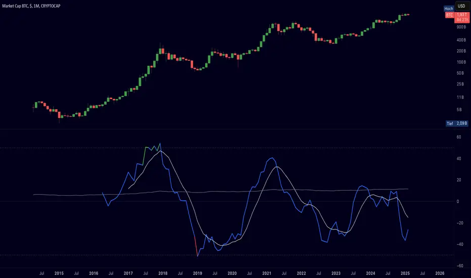
Cryptolabs Global Liquidity Cycle Momentum IndicatorCryptolabs Global Liquidity Cycle Momentum Indicator (LMI-BTC)
This open-source indicator combines global central bank liquidity data with Bitcoin price movements to identify medium- to long-term market cycles and momentum phases. It is designed for traders who want to incorporate macroeconomic factors into their Bitcoin analysis.
How It Works
The script calculates a Liquidity Index using balance sheet data from four central banks (USA: ECONOMICS:USCBBS, Japan: FRED:JPNASSETS, China: ECONOMICS:CNCBBS, EU: FRED:ECBASSETSW), augmented by the Dollar Index (TVC:DXY) and Chinese 10-year bond yields (TVC:CN10Y). This index is:
- Logarithmically scaled (math.log) to better represent large values like central bank balances and Bitcoin prices.
- Normalized over a 50-period range to balance fluctuations between minimum and maximum values.
- Compared to prior-year values, with the number of bars dynamically adjusted based on the timeframe (e.g., 252 for 1D, 52 for 1W), to compute percentage changes.
The liquidity change is analyzed using a Chande Momentum Oscillator (CMO) (period: 24) to measure momentum trends. A Weighted Moving Average (WMA) (period: 10) acts as a signal line. The Bitcoin price is also plotted logarithmically to highlight parallels with liquidity cycles.
Usage
Traders can use the indicator to:
- Identify global liquidity cycles influencing Bitcoin price trends, such as expansive or restrictive monetary policies.
- Detect momentum phases: Values above 50 suggest overbought conditions, below -50 indicate oversold conditions.
- Anticipate trend reversals by observing CMO crossovers with the signal line.
It performs best on higher timeframes like daily (1D) or weekly (1W) charts. The visualization includes:
- CMO line (green > 50, red < -50, blue neutral), signal line (white), Bitcoin price (gray).
- Horizontal lines at 50, 0, and -50 for improved readability.
Originality
This indicator stands out from other momentum tools like RSI or basic price analysis due to:
- Unique Data Integration: Combines four central bank datasets, DXY, and CN10Y as macroeconomic proxies for Bitcoin.
- Dynamic Prior-Year Analysis: Calculates liquidity changes relative to historical values, adjustable by timeframe.
- Logarithmic Normalization: Enhances visibility of extreme values, critical for cryptocurrencies and macro data.
This combination offers a rare perspective on the interplay between global liquidity and Bitcoin, unavailable in other open-source scripts.
Settings
- CMO Period: Default 24, adjustable for faster/slower signals.
- Signal WMA: Default 10, for smoothing the CMO line.
- Normalization Window: Default 50 periods, customizable.
Users can modify these parameters in the Pine Editor to tailor the indicator to their strategy.
Note
This script is designed for medium- to long-term analysis, not scalping. For optimal results, combine it with additional analyses (e.g., on-chain data, support/resistance levels). It does not guarantee profits but supports informed decisions based on macroeconomic trends.
Data Sources
- Bitcoin: INDEX:BTCUSD
- Liquidity: ECONOMICS:USCBBS, FRED:JPNASSETS, ECONOMICS:CNCBBS, FRED:ECBASSETSW
- Additional: TVC:DXY, TVC:CN10Y
Adaptive Supply and Demand [EdgeTerminal]Adaptive Supply and Demand is a dynamic supply and demand indicator with a few unique twists. It considers volume pressure, volatility-based adjustments and multi-time frame momentum for confidence scoring (multi-step confirmation) to generate dynamic lines that adjust based on the market and also to generate dynamic support/resistance levels for the supply and demand lines.
The dynamic support and resistance lines shown gives you a better situational awareness of the current state of the market and add more context to why the market is moving into a certain direction.
> Trading Scenarios
When the confidence score is over 80%, strong volume pressure in trend direction (up or down), volatility is low and momentum is aligned across timeframes, there is an indication of a strong upward or downward trend.
When the supply and demand line crossover, the confidence score is over 75% and the volume pressure is shifting, this can be an indicator of trend reversal. Use tight initial stops, scale into position as trend develops, monitor the volume pressure for continuation and wait for confidence confirmation.
When the confiance score is below 60%, the volume pressure is choppy, volatility is high, you want to avoid trading or reduce position size, wait for confidence improvements, use support and resistance for entries/exits and use tighter stops due to market conditions. This is an indication of a ranging market.
Another scenario is when there is a sudden volume pressure increase, and a raising confidence score, the volatility is expanding and the bar momentum is aligning the volatility direction. This can indicate a breakout scenario.
> How it Works
1. Volume Pressure Analysis
Volume Pressure Analysis is a key component that measures the true buying and selling force in the market. Here's a detailed breakdown. The idea is to standardize volume to prevent large spikes from skewing results.
The indicator employs an adaptive volume normalization technique to detect genuine buying and selling pressure.
It takes current volume and divides it by average volume.
If normVol > 1: Current volume is above average
If normVol < 1: Current volume is below average
An example if this would be If current volume is 1500 and average is 1000, normVol = 1.5 (50% above average)
Another component of the volume pressure analysis is the Price Change Calculation sub-module. The purpose of this is to measure price movement relative to recent average.
It works by subtracting the average price from the current price. If the value is positive, price is average and if negative, price is below average.
Finally, the volume pressure is calculated to combine volume and price for true pressure reading.
2. Savitzky-Golay Filtering
SG filtering implements advanced signal smoothing while preserving important trend features. It uses weighted moving average approximation, preserves higher moments of data and reduces noise while maintaining signal integrity.
This results in smoother signal lines, reduced false crossovers and better trend identification. Traditional moving averages tend to lag and smooth out important features. Additionally, simple moving averages can miss critical turning points and regular smoothing can delay signal generation.
SG filtering preserves higher moments such as peaks, valleys and trends, reduces noise while maintaining signal sharpness.
It works by creating a symmetric weighting scheme. This way center points get the highest weights while edge points get the lowest weight.
3. Parkinson's Volatility
Parkinson's Volatility is an advanced volatility measurement formula using high-low range data. It uses high-low range for volatility calculation, incorporates logarithmic returns and annualized the volatility measure.
This results in more accurate volatility measurement, better risk assessment and dynamic signal sensitivity.
4. Multi-timeframe Momentum
This combines signals from each module for each timeframe to calculate momentum across three timeframes. It also applies weighted importance to each timeframe and generates a composite momentum signal.
This results in a more comprehensive trend analysis, reduced timeframe bias and better trend confirmation.
> Indicator Settings
Short-term Period:
Lower values makes it more sensitive, meaning it will generate more signals. Higher values makes it less sensitive, resulting in fewer signals. We recommend a 5 to 15 range for day trading, and 10 to 20 for swing trading
Medium-term Period:
Lower values result in faster trend confirmation and higher values show slower and more reliable confirmation. We recommend a range of 15-25 for day trading and 20-30 for swing trading.
Long-term Period:
Lower values makes it more responsive to trend changes and higher values are better for major trend identification. We recommend a range of 40-60 for day trading and 50-100 for swing trading.
Volume Analysis Window:
Lower values result in more sensitivity to volume changes and higher values result in smoother volume analysis. The optimal range is 15-25 for most trading styles.
Confidence Threshold:
Lower values generate more signals but quality decreases. Higher values generate fewer signals but accuracy increases.The optimal range is 0.65-0.8 for most trading conditions.

Session Bar/Candle ColoringChange the color of candles within a user-defined trading session. Borders and wicks can be changed as well, not just the body color.
PREFACE
This script can be used an educational resource for those who are interested in learning Pine Script. Therefore, the script is published open source and is organized in a manner that follows the recommended Style Guide .
While the main premise of the indicator is rather simple, the script showcases various things that can be achieved such as conditional plotting, alignment of indicator settings, user input validation, script optimization, and more. The script also has examples of taking into consideration the chart timeframe and/or different chart types (Heikin Ashi, Renko, etc.) that a user might be running it on. Note: for complete beginners, I strongly suggest going through the Pine Script User Manual (possibly more than once).
FEATURES
Besides being able to select a specific time window, the indicator also provides additional color settings for changing the background color or changing the colors of neutral/indecisive candles, as shown in the image below.
This allows for a higher level of customization beyond the TradingView chart settings or other similar scripts that are currently available.
HOW TO USE
First, define the intraday trading session that will contain the candles to modify. The session can be limited to specific days of the week.
Next, select the parts of the candles that should be modified: Body, Borders, Wick, and/or Background.
For each of the candle parts that were enabled, you can select the colors that will be used depending on whether a candle is bullish (⇧), bearish (⇩), or neutral (⇆).
All other indicator settings will have a detailed tooltip to describe its usage and/or effect.
LIMITATIONS
The indicator is not intended to function on Daily or higher timeframes due to the intraday nature of session time windows.
The indicator cannot always automatically detect the chart type being used, therefore the user is requested to manually input the chart type via the " Chart Style " setting.
Depending on the available historical data and the selected choice for the " Portion of bar in session " setting, the indicator may not be able to update very old candles on the chart.
EXAMPLE USAGE
This section will show examples of different scenarios that the indicator can be used for.
Emphasizing a main trading session.
Defining a "Pre/post market hours background" like is available for some symbols (e.g., NASDAQ:AAPL ).
Highlighting in which bar the midnight candle occurs.
Hiding indecision bars (neutral candles).
Showing only "Regular Trading Hours" for a chart that does not have the option to toggle ETH/RTH. To achieve this, the actual chart data is hidden, and only the indicator is visible; alternatively, a 2nd instance of the indicator could change colors to match the chart background.
Using a combination of Bars and Japanese Candlesticks. Alternatively, this could be done by hiding the main chart data and using 2 instances of the indicator (one with " Chart Style " setting as Bars , and the other set to Candles ).
Using a combination of thin and thick bars on Range charts. Note: requires disabling the "Thin Bars" setting for Bar charts in the TradingView chart settings.
NOTES
If using more than one instance of this indicator on the same chart, you can use the TradingView "Save Indicator Template" feature to avoid having to re-configure the multiple indicators at a later time.
This indicator is intended to work "out-of-the-box" thanks to the behind_chart option introduced to Pine Script in October 2024. But you can always manually bring the indicator to the front just in case the color changes are not being seen (using the "More" option in the indicator status line: More > Visual Order > Bring to front ).
Many thanks to fikira for their help and inspiring me to create open source scripts.
Any feedback including bug reports or suggestions for improving the indicator (or source code itself) are always welcome in the comments section.

Time-Based VWAP (TVWAP)(TVWAP) Indicator
The Time-Based Volume Weighted Average Price (TVWAP) indicator is a customized version of VWAP designed for intraday trading sessions with defined start and end times. Unlike the traditional VWAP, which calculates the volume-weighted average price over an entire trading day, this indicator allows you to focus on specific time periods, such as ICT kill zones (e.g., London Open, New York Open, Power Hour). It helps crypto scalpers and advanced traders identify price deviations relative to volume during key trading windows.
Key Features:
Custom Time Interval:
You can set the exact start and end times for the VWAP calculation using input settings for hours and minutes (24-hour format).
Ideal for analyzing short, high-liquidity periods.
Dynamic Accumulation of Price and Volume:
The indicator resets at the beginning of the specified session and accumulates price-volume data until the end of the session.
Ensures that the TVWAP reflects the weighted average price specific to the chosen session.
Visual Representation:
The indicator plots the TVWAP line only during the specified time window, providing a clear visual reference for price action during that period.
Outside the session, the TVWAP line is hidden (na).
Use Cases:
ICT Scalp Trading:
Monitor price rebalances or potential liquidity sweeps near TVWAP during important trading sessions.
Mean Reversion Strategies:
Detect pullbacks toward the session’s average price for potential entry points.
Breakout Confirmation:
Confirm price direction relative to TVWAP during kill zones or high-volume times to determine if a breakout is supported by volume.
Inputs:
Start Hour/Minute: The time when the TVWAP calculation starts.
End Hour/Minute: The time when the TVWAP calculation ends.
Technical Explanation:
The indicator uses the timestamp function to create time markers for the session start and end.
During the session, the price-volume (close * volume) is accumulated along with the total volume.
TVWAP is calculated as:
TVWAP = (Sum of (Price × Volume)) ÷ (Sum of Volume)
Once the session ends, the TVWAP resets for the next trading period.
Customization Ideas:
Alerts: Add notifications when the price touches or deviates significantly from TVWAP.
Different Colors: Use different line colors based on upward or downward trends.
Multiple Sessions: Add support for multiple TVWAP lines for different time periods (e.g., London + New York).

Golden Time ErfanThe "Golden Time" Indicator is a custom-built TradingView tool designed to assist traders by highlighting two critical trading time windows: the New York session open and a specific strategy-based time known as Golden Time.

GMO (Gyroscopic Momentum Oscillator) GMO
Overview
This indicator fuses multiple advanced concepts to give traders a comprehensive view of market momentum, volatility, and potential turning points. It leverages the Gyroscopic Momentum Oscillator (GMO) foundation and layers on IQR-based bands, dynamic ATR-adjusted OB/OS levels, torque filtering, and divergence detection. The outcome is a versatile tool that can assist in identifying both short-term squeezes and long-term reversal zones while detecting subtle shifts in momentum acceleration.
Key Components:
Gyroscopic Momentum Oscillator (GMO) – A physics-inspired metric capturing trend stability and momentum by treating price dynamics as “angle,” “angular velocity,” and “inertia.”
IQR Bands – Highlight statistically typical oscillation ranges, providing insight into short-term squeezes and potential near-term trend shifts.
ATR-Adjusted OB/OS Levels – Dynamic thresholds for overbought/oversold conditions, adapting to volatility, aiding in identifying long-term potential reversal zones.
Torque Filtering & Scaling – Smooths and thresholds torque (the rate of change of momentum) and visually scales it for clarity, indicating sudden force changes that may precede volatility adjustments.
Divergence Detection – Highlights potential reversal cues by comparing oscillator swings against price swings, revealing regular and hidden bullish/bearish divergences.
Conceptual Insights
IQR Bands (Short-Term Squeeze & Trend Direction):
Short-Term Momentum and Squeeze: The IQR (Interquartile Range) bands show where the oscillator tends to “live” statistically. When the GMO line hovers within compressed IQR bands, it can signal a momentum squeeze phase. Exiting these tight ranges often correlates with short-term breakout opportunities.
Trend Reversals: If the oscillator pushes beyond these IQR ranges, it may indicate an emerging short-term trend change. Traders can watch for GMO escaping the IQR “comfort zone” to anticipate a new directional move.
Dynamic OB/OS Levels (Long-Term Reversal Zones):
ATR-Based Adaptive Thresholds: Instead of static overbought/oversold lines, this tool uses ATR to adjust OB/OS boundaries. In calm markets, these lines remain closer to ±90. As volatility rises, they approach ±100, reflecting greater permissible swings.
Long-Term Trend Reversal Potential: If GMO hits these dynamically adjusted OB/OS extremes, it suggests conditions ripe for possible long-term trend reversals. Traders seeking major inflection points may find these adaptive levels more reliable than fixed thresholds.
Torque (Sudden Force & Directional Shifts):
Momentum Acceleration Insight: Torque represents the second derivative of momentum, highlighting how quickly momentum is changing. High positive torque suggests a rapidly strengthening bullish force, while high negative torque warns of sudden bearish pressure.
Early Warning & Stability/Volatility Adjustments: By monitoring torque spikes, traders can anticipate momentum shifts before price fully confirms them. This can signal imminent changes in stability or increased volatility phases.
Indicator Parameters and Usage
GMO-Related Inputs:
lenPivot (Default 100): Length for calculating the pivot line (slow market axis).
lenSmoothAngle (Default 200): Smooths the angle measure, reducing noise.
lenATR (Default 14): ATR period for scaling factor, linking price changes to volatility.
useVolatility (Default true): If true, volatility (ATR) influences inertia, adjusting momentum calculations.
useVolume (Default false): If true, volume affects inertia, adding a liquidity dimension to momentum.
lenVolSmoothing (Default 50): Smooths volume calculations if useVolume is enabled.
lenMomentumSmooth (Default 20): EMA smoothing of GMO for a cleaner oscillator line.
normalizeRange (Default true): Normalizes GMO to a fixed range for consistent interpretation.
lenNorm (Default 100): Length for normalization window, ensuring GMO’s scale adapts to recent extremes.
IQR Bands Settings:
iqrLength (Default 14): Period to compute the oscillator’s statistical IQR.
iqrMult (Default 1.5): Multiplier to define the upper and lower IQR-based bands.
ATR-Adjusted OB/OS Settings:
baseOBLevel (Fixed at 90) and baseOSLevel (Fixed at 90): Base lines for OB/OS.
atrPeriodForOBOS (Default 50): ATR length for adjusting OB/OS thresholds dynamically.
atrScaling (Default 0.2): Controls how strongly volatility affects OB/OS lines.
Torque Filtering & Visualization:
torqueSmoothLength (Default 10): EMA length to smooth raw torque values.
atrPeriodForTorque (Default 14): ATR period to determine torque threshold.
atrTorqueScaling (Default 0.5): Scales ATR for determining torque’s “significant” threshold.
torqueScaleFactor (Default 10.0): Multiplies the torque values for better visual prominence on the chart.
Divergence Inputs:
showDivergences (Default true): Toggles divergence signals.
lbR, lbL (Defaults 5): Pivot lookback periods to identify swing highs and lows.
rangeUpper, rangeLower: Bar constraints to validate potential divergences.
plotBull, plotHiddenBull, plotBear, plotHiddenBear: Toggles for each divergence type.
Visual Elements on the Chart
GMO Line (Blue) & Zero Line (Gray):
GMO line oscillates around zero. Positive territory hints bullish momentum, negative suggests bearish.
IQR Bands (Teal Lines & Yellow Fill):
Upper/lower bands form a statistical “normal range” for GMO. The median line (purple) provides a central reference. Contraction near these bands indicates a short-term squeeze, expansions beyond them can signal emerging short-term trend changes.
Dynamic OB/OS (Red & Green Lines):
Red line near +90 to +100: Overbought zone (dynamic).
Green line near -90 to -100: Oversold zone (dynamic).
Movement into these zones may mark significant, longer-term reversal potential.
Torque Histogram (Colored Bars):
Plotted below GMO. Green bars = torque above positive threshold (bullish acceleration).
Red bars = torque below negative threshold (bearish acceleration).
Gray bars = neutral range.
This provides early warnings of momentum shifts before price responds fully.
Precession (Orange Line):
Scaled for visibility, adds context to long-term angular shifts in the oscillator.
Divergence Signals (Shapes):
Circles and offset lines highlight regular or hidden bullish/bearish divergences, offering potential reversal signals.
Practical Interpretation & Strategy
Short-Term Opportunities (IQR Focus):
If GMO compresses within IQR bands, the market might be “winding up.” A break above/below these bands can signal a short-term trade opportunity.
Long-Term Reversal Zones (Dynamic OB/OS):
When GMO approaches these dynamically adjusted extremes, conditions may be ripe for a major trend shift. This is particularly useful for swing or position traders looking for significant turnarounds.
Monitoring Torque for Acceleration Cues:
Torque spikes can precede price action, serving as an early catalyst signal. If torque turns strongly positive, anticipate bullish acceleration; strongly negative torque may warn of upcoming bearish pressure.
Confirm with Divergences:
Divergences between price and GMO reinforce potential reversal or continuation signals identified by IQR, OB/OS, or torque. Use them to increase confidence in setups.
Tips and Best Practices
Combine with Price & Volume Action:
While the indicator is powerful, always confirm signals with actual price structure, volume patterns, or other trend-following tools.
Adjust Lengths & Periods as Needed:
Shorter lengths = more responsiveness but more noise. Longer lengths = smoother signals but greater lag. Tune parameters to match your trading style and timeframe.
Use ATR and Volume Settings Wisely:
If markets are highly volatile, consider useVolatility to refine momentum readings. If liquidity is key, enable useVolume.
Scaling Torque:
If torque bars are hard to read, increase torqueScaleFactor further. The scaling doesn’t affect logic—only visibility.
Conclusion
The “GMO + IQR Bands + ATR-Adjusted OB/OS + Torque Filtering (Scaled)” indicator presents a holistic framework for understanding market momentum across multiple timescales and conditions. By interpreting short-term squeezes via IQR bands, long-term reversal zones via adaptive OB/OS, and subtle acceleration changes through torque, traders can gain advanced insights into when to anticipate breakouts, manage risk around potential reversals, and fine-tune timing for entries and exits.
This integrated approach helps navigate complex market dynamics, making it a valuable addition to any technical analysis toolkit.
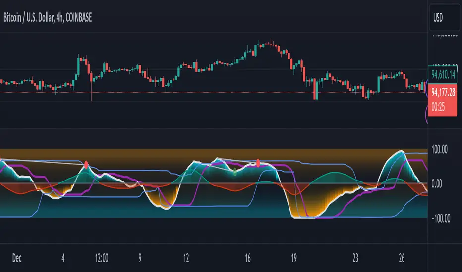
Custom ATR with Paranormal Bar FilterCustom ATR with Paranormal Bar Filter
Description:
This indicator calculates a custom ATR (Average True Range) by filtering out bars with unusually large or small price ranges. It helps provide a more accurate measure of market volatility by ignoring outliers.
How it works:
True Range Calculation:
The price range for each bar is calculated.
Bars with ranges much larger or smaller than typical are excluded.
Filtered ATR:
The ATR is calculated using only the bars that pass the filter.
Current Bar Progress:
Measures how much the current bar has moved compared to the filtered ATR, based on the difference between its opening and closing prices.
Display:
A line represents the filtered ATR.
A table shows the filtered ATR, the current bar's range, and its progress relative to the ATR.
Input Settings:
ATR Period: Number of bars used to calculate the ATR.
Filter Window: Number of recent bars used to determine the typical range.
Filter Threshold: Sensitivity of the filter. A higher value allows more bars to pass.
How to Use:
Monitor Volatility:
Use the filtered ATR to understand market volatility while ignoring unusual price movements.
Track Current Bar Progress:
See how much of the ATR the current bar has completed.
Adjust Filter Settings:
Fine-tune the filter to match your trading timeframe and strategy.
This indicator is designed for traders who want to track market volatility without being misled by extreme outlier bars.

High/Low Location Frequency [LuxAlgo]The High/Low Location Frequency tool provides users with probabilities of tops and bottoms at user-defined periods, along with advanced filters that offer deep and objective market information about the likelihood of a top or bottom in the market.
🔶 USAGE
There are four different time periods that traders can select for analysis of probabilities:
HOUR OF DAY: Probability of occurrence of top and bottom prices for each hour of the day
DAY OF WEEK: Probability of occurrence of top and bottom prices for each day of the week
DAY OF MONTH: Probability of occurrence of top and bottom prices for each day of the month
MONTH OF YEAR: Probability of occurrence of top and bottom prices for each month
The data is displayed as a dashboard, which users can position according to their preferences. The dashboard includes useful information in the header, such as the number of periods and the date from which the data is gathered. Additionally, users can enable active filters to customize their view. The probabilities are displayed in one, two, or three columns, depending on the number of elements.
🔹 Advanced Filters
Advanced Filters allow traders to exclude specific data from the results. They can choose to use none or all filters simultaneously, inputting a list of numbers separated by spaces or commas. However, it is not possible to use both separators on the same filter.
The tool is equipped with five advanced filters:
HOURS OF DAY: The permitted range is from 0 to 23.
DAYS OF WEEK: The permitted range is from 1 to 7.
DAYS OF MONTH: The permitted range is from 1 to 31.
MONTHS: The permitted range is from 1 to 12.
YEARS: The permitted range is from 1000 to 2999.
It should be noted that the DAYS OF WEEK advanced filter has been designed for use with tickers that trade every day, such as those trading in the crypto market. In such cases, the numbers displayed will range from 1 (Sunday) to 7 (Saturday). Conversely, for tickers that do not trade over the weekend, the numbers will range from 1 (Monday) to 5 (Friday).
To illustrate the application of this filter, we will exclude results for Mondays and Tuesdays, the first five days of each month, January and February, and the years 2020, 2021, and 2022. Let us review the results:
DAYS OF WEEK: `2,3` or `2 3` (for crypto) or `1,2` or `1 2` (for the rest)
DAYS OF MONTH: `1,2,3,4,5` or `1 2 3 4 5`
MONTHS: `1,2` or `1 2`
YEARS: `2020,2021,2022` or `2020 2021 2022`
🔹 High Probability Lines
The tool enables traders to identify the next period with the highest probability of a top (red) and/or bottom (green) on the chart, marked with two horizontal lines indicating the location of these periods.
🔹 Top/Bottom Labels and Periods Highlight
The tool is capable of indicating on the chart the upper and lower limits of each selected period, as well as the commencement of each new period, thus providing traders with a convenient reference point.
🔶 SETTINGS
Period: Select how many bars (hours, days, or months) will be used to gather data from, max value as default.
Execution Window: Select how many bars (hours, days, or months) will be used to gather data from
🔹 Advanced Filters
Hours of day: Filter which hours of the day are excluded from the data, it accepts a list of hours from 0 to 23 separated by commas or spaces, users can not mix commas or spaces as a separator, must choose one
Days of week: Filter which days of the week are excluded from the data, it accepts a list of days from 1 to 5 for tickers not trading weekends, or from 1 to 7 for tickers trading all week, users can choose between commas or spaces as a separator, but can not mix them on the same filter.
Days of month: Filter which days of the month are excluded from the data, it accepts a list of days from 1 to 31, users can choose between commas or spaces as separator, but can not mix them on the same filter.
Months: Filter months to exclude from data. Accepts months from 1 to 12. Choose one separator: comma or space.
Years: Filter years to exclude from data. Accepts years from 1000 to 2999. Choose one separator: comma or space.
🔹 Dashboard
Dashboard Location: Select both the vertical and horizontal parameters for the desired location of the dashboard.
Dashboard Size: Select size for dashboard.
🔹 Style
High Probability Top Line: Enable/disable `High Probability Top` vertical line and choose color
High Probability Bottom Line: Enable/disable `High Probability Bottom` vertical line and choose color
Top Label: Enable/disable period top labels, choose color and size.
Bottom Label: Enable/disable period bottom labels, choose color and size.
Highlight Period Changes: Enable/disable vertical highlight at start of period

Larry Williams Valuation Index [tradeviZion]Larry Williams Valuation Index
Welcome to the Larry Williams Valuation Index by tradeviZion! This script is an interpretation of Larry Williams' famous WillVal (Valuation) Index, originally developed in 1990 to help traders determine whether a market or asset is overvalued or undervalued. We've extended it to support multiple securities and offer alerts for different valuation levels, helping you make more informed trading decisions.
What is the Valuation Index?
The Valuation Index measures how a security's current price compares to its historical price action. It helps identify whether the security is overvalued (priced too high), undervalued (priced too low), or in a normal range.
This version supports multiple securities and uses valuation parameters to help you assess the relative valuation of three securities simultaneously. It can help you determine the best times to enter (buy) or exit (sell) the market.
Key Features
Multi-Security Analysis: Analyze up to three securities simultaneously to get a broader view of market conditions.
Valuation Levels: Automatically calculate overvaluation and undervaluation levels or set manual levels for consistent analysis.
Custom Alerts: Create custom alerts when securities move between overvalued, undervalued, or normal ranges.
Customizable Table Display: Display a table with valuation values and their status on the chart.
Getting Started
Step 1: Adding the Script to Your Chart
First, add the Larry Williams Valuation Index script to your chart on TradingView. The script is designed to work with any timeframe, but for best results, use weekly or daily timeframes for a longer-term perspective.
Step 2: Configuring Securities
The script allows you to analyze up to three different securities :
Security 1 (Default: DXY)
Security 2 (Default: GC1!)
Security 3 (Default: ZB1!)
You can enable or disable each security individually.
Custom Timeframe Option: You have the option to select a custom timeframe for analysis. This allows you to see whether the security is overvalued or undervalued in lower or higher timeframes. Note that this feature is experimental and has not been extensively tested. Larry Williams originally used the weekly timeframe to determine if a stock was overvalued or undervalued. By default, the indicator compares the current price with the security based on the selected timeframe, except if you choose to use a custom timeframe.
Pro Tip : New users can start with the default securities to understand the concept before using other assets.
Step 3: Valuation Index Settings
Short EMA Length : This is the short-term average used for calculations. A lower value makes it more responsive to recent price changes.
Long EMA Length : This is the long-term average, used to smooth the valuation over time.
Valuation Length (Default: 156) : Represents approximately three years of daily bars (as recommended by Larry Williams).
How is the Valuation Index Calculated?
The valuation calculation is done using a method called WVI (WillVal Index), which compares the current price of a security to the price of another correlated security. Here’s a step-by-step explanation:
1. Data Collection: The script takes the closing price of the security you are analyzing and the closing price of the correlated security.
2. Ratio Calculation : The ratio of the two prices is calculated:
Price Ratio = (Price of your security) / (Price of correlated security) * 100.
This ratio helps determine how expensive or cheap your security is compared to the correlated one.
3. Exponential Moving Averages (EMAs) : The price ratio is used to calculate short-term and long-term EMAs (Exponential Moving Averages). EMAs are used to create smooth lines that represent the average price of a security over a specific period of time, with more weight given to recent data. By calculating both short-term and long-term EMAs, we can identify the trend direction and how the security is performing compared to its historical averages.
4. Valuation Index Calculation:
The Valuation Index is calculated as the difference between the short-term EMA and the long-term EMA. This difference helps to determine if the security is currently overvalued or undervalued:
A positive value indicates that the price is above its longer-term trend, suggesting potential overvaluation.
A negative value indicates that the price is below its longer-term trend, suggesting potential undervaluation.
5. Normalization:
To make the valuation easier to interpret, the calculated valuation index is then normalized using the highest and lowest values over the selected valuation length (e.g., 156 bars).
This normalization process converts the index into a percentage between 0 and 100, where higher values indicate overvaluation and lower values indicate undervaluation.
Step 4: Understanding Valuation Levels
The valuation levels indicate whether a security is currently undervalued, overvalued, or in a normal range.
Manual Levels : You can manually set the overvaluation and undervaluation thresholds (default is 85 for overvalued and 15 for undervalued).
Auto Levels : The script can automatically calculate these levels based on recent price action, allowing you to adapt to changing market conditions.
Auto Levels Calculation Explained:
The Auto Levels are calculated by taking the average of the valuation indices for all three securities (e.g., index1, index2, and index3).
The script then looks at the highest and lowest values of this average over a selected number of recent bars (e.g., 50 bars).
The overvaluation level is determined by taking the highest value and multiplying it by a multiplier (e.g., 5). Similarly, the undervaluation level is calculated using the lowest value and the multiplier.
These dynamic levels adjust according to recent price action, providing an adaptive approach to identifying overvalued and undervalued conditions.
Step 5: How to Use the Script to Make Trading Decisions
For new users, here's a step-by-step trading strategy you can use with the Valuation Index:
1. Identify Undervalued Opportunities
When two or more securities are in the undervalued range (below 15 for manual or below automatically calculated undervalue levels), wait for at least two of these securities to turn from undervalued to normal .
This transition indicates a potential buy opportunity .
2. Buying Signal
When at least two securities transition from undervalued to normal, you can consider buying the asset.
This indicates that the market may be recovering from undervalued conditions and could be moving into a growth phase.
3. Selling Signal
Exit when the price high closes below the EMA 21 (21-day exponential moving average).
Alternatively, if the valuation index reaches overvalued levels (above 85 manually or auto-calculated), wait for it to drop back to normal . This can be another point to exit the trade .
You can also use any other sell condition based on your r isk management strategy .
Alerts for Valuation Levels
The script includes alerts to notify you of changing market conditions:
To activate these alerts, follow these steps, referring to the provided screenshot with detailed steps:
1. Enable Alerts : Click on the settings gear icon on the script title in your chart. In the settings menu, scroll to the section labeled Alerts Settings .
Enable Alerts by checking the Enable Alerts box.
Set the Required Securities for Alert (default is 2 securities).
Choose the Alert Frequency : Selecting Once Per Bar Close will trigger alerts only at the close of each bar, ensuring you receive confirmed signals rather than potentially noisy intermediate signals.
2. Select Alert Type : Choose the type of alert you want to activate, such as Alert on Overvalued, Alert on Undervalued, Alert on Over to Normal , or Alert on Under to Normal .
3. Save Settings : Click OK to save your alert settings.
4. Add Alert on Indicator : Click the "..." (More button) next to the indicator name on the chart and select " Add alert on tradeviZion - WillVal ".
5. Create Alert : In the Create Alert window:
Set Condition to tradeviZion - WillVal .
Ensure Any alert() function call is selected.
Set the Alert Name and select your Expiration preferences.
6. Set Notification Preferences : Go to the Notifications tab and select how you want to receive notifications, such as via app notification, toast notification, email , or sound alert . Adjust these preferences to best suit your needs.
7. Click Create : Finally, click Create to activate the alert.
These alerts will help you stay informed about key market conditions and take action accordingly, ensuring you do not miss critical trading opportunities.
Understanding the Table Display
The script includes an interactive table on the chart to show the valuation status of each security:
Security : The name of the security being analyzed.
Value : The current valuation index value.
Status : Indicates whether the security is overvalued, undervalued , or in a normal range.
Color: Displays a color code for easy identification of status:
Red for overvalued.
Green for undervalued.
Other colors represent normal valuation levels.
Empowering Messages : Motivational messages are displayed to encourage disciplined trading. These messages will change periodically, helping keep a positive trading mindset.
Acknowledgment
This tool builds upon the foundational work of Larry Williams, who developed the WillVal (Valuation) Index concept. It also incorporates enhancements to extend multi-security analysis, valuation normalization, and advanced alerting features, providing a more versatile and powerful indicator. The Larry Williams Valuation Index [ tradeviZion ] helps traders make informed decisions by assessing overvalued and undervalued conditions for multiple securities simultaneously.
Note : Always practice proper risk management and thoroughly test the indicator to ensure it aligns with your trading strategy. Past performance is not indicative of future results.
Trade smarter with TradeVizion—unlock your trading potential today!

The Vet [TFO]In collaboration with @mickey1984 , "The Vet" was created to showcase various statistical measures of price.
The first core measurement utilizes the Defining Range (DR) concept on a weekly basis. For example, we might track the session from 09:30-10:30 on Mondays to get the DR high, DR low, IDR high, and IDR low. The DR high and low are the highest high and lowest low of the session, respectively, whereas the IDR high and low would be the highest candle body level (open or close) and lowest candle body level, respectively, during this window of time.
From this data, we use the IDR range (from IDR high to IDR low) to extrapolate several, custom projections of this range from its high and low so that we can collect data on how often these levels are hit, from the close of one DR session to the open of the next one.
This information is displayed in the Range Projection Table with a few main columns of information:
- The leftmost column indicates each level that is projected from the IDR range, where (+) indicates a projection above the range high, and (-) indicates a projection below the range low
- The "First Touch" column indicates how often price has reached these levels in the past at any point until the next weekly DR session
- The "Other Side Touch" column indicates how often price has reached a given level, then reversed to hit the opposing level of the same magnitude. For example, the above chart shows that if price hit the +1 projection, ~33% of instances also hit the -1 projection before the next weekly DR session. For this reason, the probabilities will be the same for projection levels of the same but opposite magnitude (+1 would be the same as -1, +3 would be the same as -3, etc.)
- The "Next Level Touch" column provides insight into how often price reaches the next greatest projection level. For example, in the above chart, the red box in the projection table is highlighting that once price hits the -2 projection, ~86% of instances reached the -3 projection before the next weekly DR session
- The last columns, "Within ADR" and "Within AWR" show if any of the projection levels are within the current Average Daily Range, or Average Weekly Range, respectively, which can both be enabled from the Average Range section
The next section, Distributions, primarily measures and displays the average price movements from specified intraday time windows. The option to Show Distribution Boxes will overlay a box showing each respective session's average range, while adjusting itself to encapsulate the price action of that session until the average range is met/exceeded. Users can choose to display the range average by Day of Week, or the Total average from all days. Values for average ranges can either be shown as point or percent values. We can also show a table to display this information about price's average ranges for each given session, and show labels displaying the current range vs its average.
The final section, Average Range, simply offers the ability to plot the Average Daily Range (ADR) and Average Weekly Range (AWR) of a specified length. An ADR of 10 for example would take the average of the last 10 days, from high to low, while an AWR of 10 would take the average of the last 10 weeks (if the current chart provides enough data to support this). Similarly, we can also show the Average Range Table to indicate what these ADR/AWR values are, what our current range is and how it compares to those values, as well as some simple statistics on how often these levels are hit. As an example, "Hit +/- ADR: 40%/35%" in this table would indicate that price has hit the upper ADR limit 40% of the time, and the lower limit 35% of the time, for the amount of data available on the current chart.
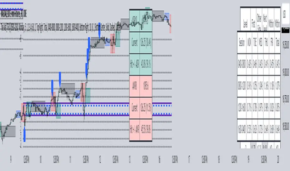
Price Action Smart Money Concepts [BigBeluga]THE SMART MONEY CONCEPTS Toolkit
The Smart Money Concepts [ BigBeluga ] is a comprehensive toolkit built around the principles of "smart money" behavior, which refers to the actions and strategies of institutional investors.
The Smart Money Concepts Toolkit brings together a suite of advanced indicators that are all interconnected and built around a unified concept: understanding and trading like institutional investors, or "smart money." These indicators are not just randomly chosen tools; they are features of a single overarching framework, which is why having them all in one place creates such a powerful system.
This all-in-one toolkit provides the user with a unique experience by automating most of the basic and advanced concepts on the chart, saving them time and improving their trading ideas.
Real-time market structure analysis simplifies complex trends by pinpointing key support, resistance, and breakout levels.
Advanced order block analysis leverages detailed volume data to pinpoint high-demand zones, revealing internal market sentiment and predicting potential reversals. This analysis utilizes bid/ask zones to provide supply/demand insights, empowering informed trading decisions.
Imbalance Concepts (FVG and Breakers) allows traders to identify potential market weaknesses and areas where price might be attracted to fill the gap, creating opportunities for entry and exit.
Swing failure patterns help traders identify potential entry points and rejection zones based on price swings.
Liquidity Concepts, our advanced liquidity algorithm, pinpoints high-impact events, allowing you to predict market shifts, strong price reactions, and potential stop-loss hunting zones. This gives traders an edge to make informed trading decisions based on liquidity dynamics.
🔵 FEATURES
The indicator has quite a lot of features that are provided below:
Swing market structure
Internal market structure
Mapping structure
Adjustable market structure
Strong/Weak H&L
Sweep
Volumetric Order block / Breakers
Fair Value Gaps / Breakers (multi-timeframe)
Swing Failure Patterns (multi-timeframe)
Deviation area
Equal H&L
Liquidity Prints
Buyside & Sellside
Sweep Area
Highs and Lows (multi-timeframe)
🔵 BASIC DEMONSTRATION OF ALL FEATURES
1. MARKET STRUCTURE
The preceding image illustrates the market structure functionality within the Smart Money Concepts indicator.
➤ Solid lines: These represent the core indicator's internal structure, forming the foundation for most other components. They visually depict the overall market direction and identify major reversal points marked by significant price movements (denoted as 'x').
➤ Internal Structure: These represent an alternative internal structure with the potential to drive more rapid market shifts. This is particularly relevant when a significant gap exists in the established swing structure, specifically between the Break of Structure (BOS) and the most recent Change of High/Low (CHoCH). Identifying these formations can offer opportunities for quicker entries and potential short-term reversals.
➤ Sweeps (x): These signify potential turning points in the market where liquidity is removed from the structure. This suggests a possible trend reversal and presents crucial entry opportunities. Sweeps are identified within both swing and internal structures, providing valuable insights for informed trading decisions.
➤ Mapping structure: A tool that automatically identifies and connects significant price highs and lows, creating a zig-zag pattern. It visualizes market structure, highlights trends, support/resistance levels, and potential breakouts. Helps traders quickly grasp price action patterns and make informed decisions.
➤ Color-coded candles based on market structure: These colors visually represent the underlying market structure, making it easier for traders to quickly identify trends.
➤ Extreme H&L: It visualizes market structure with extreme high and lows, which gives perspective for macro Market Structure.
2. VOLUMETRIC ORDER BLOCKS
Order blocks are specific areas on a financial chart where significant buying or selling activity has occurred. These are not just simple zones; they contain valuable information about market dynamics. Within each of these order blocks, volume bars represent the actual buying and selling activity that took place. These volume bars offer deeper insights into the strength of the order block by showing how much buying or selling power is concentrated in that specific zone.
Additionally, these order blocks can be transformed into Breaker Blocks. When an order block fails—meaning the price breaks through this zone without reversing—it becomes a breaker block. Breaker blocks are particularly useful for trading breakouts, as they signal that the market has shifted beyond a previously established zone, offering opportunities for traders to enter in the direction of the breakout.
Here's a breakdown:
➤ Bear Order Blocks (Red): These are zones where a lot of selling happened. Traders see these areas as places where sellers were strong, pushing the price down. When the price returns to these zones, it might face resistance and drop again.
➤ Bull Order Blocks (Green): These are zones where a lot of buying happened. Traders see these areas as places where buyers were strong, pushing the price up. When the price returns to these zones, it might find support and rise again.
These Order Blocks help traders identify potential areas for entering or exiting trades based on past market activity. The volume bars inside blocks show the amount of trading activity that occurred in these blocks, giving an idea of the strength of buying or selling pressure.
➤ Breaker Block: When an order block fails, meaning the price breaks through this zone without reversing, it becomes a breaker block. This indicates a significant shift in market liquidity and structure.
➤ A bearish breaker block occurs after a bullish order block fails. This typically happens when there's an upward trend, and a certain level that was expected to support the market's rise instead gives way, leading to a sharp decline. This decline indicates that sellers have overcome the buyers, absorbing liquidity and shifting the sentiment from bullish to bearish.
Conversely, a bullish breaker block is formed from the failure of a bearish order block. In a downtrend, when a level that was expected to act as resistance is breached, and the price shoots up, it signifies that buyers have taken control, overpowering the sellers.
3. FAIR VALUE GAPS:
A fair value gap (FVG), also referred to as an imbalance, is an essential concept in Smart Money trading. It highlights the supply and demand dynamics. This gap arises when there's a notable difference between the volume of buy and sell orders. FVGs can be found across various asset classes, including forex, commodities, stocks, and cryptocurrencies.
FVGs in this toolkit have the ability to detect raids of FVG which helps to identify potential price reversals.
Mitigation option helps to change from what source FVGs will be identified: Close, Wicks or AVG.
4. SWING FAILURE PATTERN (SFP):
The Swing Failure Pattern is a liquidity engineering pattern, generally used to fill large orders. This means, the SFP generally occurs when larger players push the price into liquidity pockets with the sole objective of filling their own positions.
SFP is a technical analysis tool designed to identify potential market reversals. It works by detecting instances where the price briefly breaks a previous high or low but fails to maintain that breakout, quickly reversing direction.
How it works:
Pattern Detection: The indicator scans for price movements that breach recent highs or lows.
Reversal Confirmation: If the price quickly reverses after breaching these levels, it's identified as an SFP.
➤ SFP Display:
Bullish SFP: Marked with a green symbol when price drops below a recent low before reversing upwards.
Bearish SFP: Marked with a red symbol when price rises above a recent high before reversing downwards.
➤ Deviation Levels: After detecting an SFP, the indicator projects white lines showing potential price deviation:
For bullish SFPs, the deviation line appears above the current price.
For bearish SFPs, the deviation line appears below the current price.
These deviation levels can serve as a potential trading opportunity or areas where the reversal might lose momentum.
With Volume Threshold and Filtering of SFP traders can adjust their trading style:
Volume Threshold: This setting allows traders to filter SFPs based on the volume of the reversal candle. By setting a higher volume threshold, traders can focus on potentially more significant reversals that are backed by higher trading activity.
SFP Filtering: This feature enables traders to filter SFP detection. It includes parameters such as:
5. LIQUIDITY CONCEPTS:
➤ Equal Lows (EQL) and Equal Highs (EQH) are important concepts in liquidity-based trading.
EQL: A series of two or more swing lows that occur at approximately the same price level.
EQH: A series of two or more swing highs that occur at approximately the same price level.
EQLs and EQHs are seen as potential liquidity pools where a large number of stop loss orders or limit orders may be clustered. They can be used as potential reverse points for trades.
This multi-period feature allows traders to select less and more significant EQL and EQH:
➤ Liquidity wicks:
Liquidity wicks are a minor representation of a stop-loss hunt during the retracement of a pivot point:
➤ Buy and Sell side liquidity:
The buy side liquidity represents a concentration of potential buy orders below the current price level. When price moves into this area, it can lead to increased buying pressure due to the execution of these orders.
The sell side liquidity indicates a pool of potential sell orders below the current price level. Price movement into this area can result in increased selling pressure as these orders are executed.
➤ Sweep Liquidation Zones:
Sweep Liquidation Zones are crucial for understanding market structure and potential future price movements. They provide insights into areas where significant market participants have been forced out of their positions, potentially setting up new trading opportunities.
🔵 USAGE & EXAMPLES
The core principle behind the success of this toolkit lies in identifying "confluence." This refers to the convergence of multiple trading indicators all signaling the same information at a specific point or area. By seeking such alignment, traders can significantly enhance the likelihood of successful trades.
MS + OBs
The chart illustrates a highly bullish setup where the price is rejecting from a bullish order block (POC), while simultaneously forming a bullish Swing Failure Pattern (SFP). This occurs after an internal structure change, marked by a bullish Change of Character (CHoCH). The price broke through a bearish order block, transforming it into a breaker block, further confirming the bullish momentum.
The combination of these elements—bullish order blocks, SFP, and CHoCH—creates a powerful bullish signal, reinforcing the potential for upward movement in the market.
SFP + Bear OB
This chart above displays a bearish setup with a high probability of a price move lower. The price is currently rejecting from a bear order block, which represents a key resistance area where significant selling pressure has previously occurred. A Swing Failure Pattern (SFP) has also formed near this bear order block, indicating that the price briefly attempted to break above a recent high but failed to sustain that upward movement. This failure suggests that buyers are losing momentum, and the market could be preparing for a move to the downside.
Additionally, we can toggle on the Deviation Area in the SFP section to highlight potential levels where price deviation might occur. These deviation areas represent zones where the price is likely to react after the Swing Failure Pattern:
BUY – SELL sides + EQL
The chart showcases a bullish setup with a high probability of price breaking out of the current sell-side resistance level. The market structure indicates a formation of Equal Lows (EQL), which often suggests a build-up of liquidity that could drive the price higher.
The presence of strong buy-side pressure (69%), indicated by the green zone at the bottom, reinforces this bullish outlook. This area represents a key support zone where buyers are outpacing sellers, providing the foundation for a potential upward breakout.
EQL + Bull ChoCh
This chart illustrates a potential bullish setup, driven by the formation of Equal Lows (EQL) followed by a bullish Change of Character (CHoCH). The presence of Equal Lows often signals a liquidity build-up, which can lead to a reversal when combined with additional bullish signals.
Liquidity grab + Bull ChoCh + FVGs
This chart demonstrates a strong bullish scenario, where several important market dynamics are at play. The price begins its upward momentum from Liquidity grab following a bullish Change of Character (CHoCH), signaling the transition from a bearish phase to a bullish one.
As the price progresses, it performs liquidity grabs, which serve to gather the necessary fuel for further movement. These liquidity grabs often occur before significant price surges, as large market participants exploit these areas to accumulate positions before pushing the price higher.
The chart also highlights a market imbalance area, showing strong momentum as the price moves swiftly through this zone.
In this examples, we see how the combination of multiple “smart money” tools helps identify a potential trade opportunities. This is just one of the many scenarios that traders can spot using this toolkit. Other combinations—such as order blocks, liquidity grabs, fair value gaps, and Swing Failure Patterns (SFPs)—can also be layered on top of these concepts to further refine your trading strategy.
🔵 SETTINGS
Window: limit calculation period
Swing: limit drawing function
Mapping structure: show structural points
Algorithmic Logic: (Extreme-Adjusted) Use max high/low or pivot point calculation
Algorithmic loopback: pivot point look back
Show Last: Amount of Order block to display
Hide Overlap: hide overlapping order blocks
Construction: Size of the order blocks
Fair value gaps: Choose between normal FVG or Breaker FVG
Mitigation: (close - wick - avg) point to mitigate the order block/imbalance
SFP lookback: find a higher / lower point to improve accuracy
Threshold: remove less relevant SFP
Equal H&L: (short-mid-long term) display longer term
Liquidity Prints: Shows wicks of candles where liquidity was grabbed
Sweep Area: Identify Sweep Liquidation areas
By combining these indicators in one toolkit, traders are equipped with a comprehensive suite of tools that address every angle of the Smart Money Concept. Instead of relying on disparate tools spread across various platforms, having them integrated into a single, cohesive system allows traders to easily see confluence and make more informed trading decisions.

Momentum Alligator 4h Bitcoin StrategyOverview
The Momentum Alligator 4h Bitcoin Strategy is a trend-following trading system that operates on dual time frames. It utilizes the 1D Williams Alligator indicator to identify the prevailing major price trend and seeks trading opportunities on the 4-hour (4h) time frame when the momentum is turning up. The strategy is designed to close trades if the trend fails to develop or holding position if price continues increasing without any significant correction. Note that this strategy is specifically tailored for the 4-hour time frame.
Unique Features
2-layers market noise filtering system: Trades are only initiated in the direction of the 1D trend, determined by the Williams Alligator indicator. This higher time frame confirmation filters out minor trade signals, focusing on more substantial opportunities. At the same time, strategy has additional filter on 4h time frame with Awesome Oscillator which is showing the current price momentum.
Flexible Risk Management: The strategy exclusively opens long positions, resulting in fewer trades during bear markets. It incorporates a dynamic stop-loss mechanism, which can either follow the jaw line of the 4h Alligator or a user-defined fixed stop-loss. This flexibility helps manage risk and avoid non-trending markets.
Methodology
The strategy initiates a long position when the d-line of Stochastic RSI crosses up it's k-line. It means that there is a high probability that price momentum reversed from down to up. To avoid overtrading in potentially choppy markets, it skips the next two trades following a winning trade, anticipating sideways movement after a significant price surge.
This strategy has two layers trades filtering system: 4h and 1D time frames. The first one is awesome oscillator. It shall be increasing and value has to be higher than it's 5-period SMA. This is an additional confirmation that long trade is opened in the direction of the current momentum. As it was mentioned above, all entry signals are validated against the 1D Williams Alligator indicator. A trade is only opened if the price is above all three lines of the 1D Alligator, ensuring alignment with the major trend.
A trade is closed if the price hits the 4h jaw line of the Alligator or reaches the user-defined stop-loss level.
Risk Management
The strategy employs a combined approach to risk management:
It allows positions to ride the trend as long as the price continues to move favorably, aiming to capture significant price movements. It features a user-defined stop-loss parameter to mitigate risks based on individual risk tolerance. By default, this stop-loss is set to a 2% drop from the entry point, but it can be adjusted according to the trader's preferences.
Justification of Methodology
This strategy leverages Stochastic RSI on 4h time frame to open long trade when momentum started reversing to the upside. On the one hand, Stochastic RSI is one of the most sensitive indicator, which allows to react fast on the potential trend reversal. On the other hand, this indicator can be too sensitive and provide a lot of false trend changing signals. To eliminate this weakness we use two-layers trades filtering system.
The first layer is the 4h Awesome oscillator. This is less sensitive momentum indicator. Usually it starts increasing when price has already passed significant distance from the actual reversal point. The strategy opens long trade only is Awesome oscillator is increasing and above it's 5-period SMA. This approach increases the probability to filter the false signals during the choppy market or if the reversal is false.
The second layer filter is the Williams Alligator indicator on 1D time frame. The 1D Alligator serves as a filter for identifying the primary trend and increases probability to avoid the trades with low potential because trading against major trend usually is more risky. It's much better to catch the trend continuation than local bounce.
Last but not least feature of this strategy is close trades condition. It uses the flexible approach. First of all, user can set up the fixed stop-loss according to his own risk-tolerance, by default this value is 2% of price movement. It restricts the potential loss at the moment when trade has just been opened. Moreover strategy utilizes the 4h Williams Alligator's jaw line to exit the trade. If price fell below it trade is closed. This approach helps to not keep open trade if trend is not developing and hold it if price continues going up.
Backtest Results:
Operating window: Date range of backtests is 2021.01.01 - 2024.05.01. It is chosen to let the strategy to close all opened positions.
Commission and Slippage: Includes a standard Binance commission of 0.1% and accounts for possible slippage over 5 ticks.
Initial capital: 10000 USDT
Percent of capital used in every trade: 50%
Maximum Single Position Loss: -3.04%
Maximum Single Profit: +29.67%
Net Profit: +6228.01 USDT (+62.28%)
Total Trades: 118 (24.58% win rate)
Profit Factor: 1.71
Maximum Accumulated Loss: 1527.69 USDT (-11.52%)
Average Profit per Trade: 52.78 USDT (+0.89%)
Average Trade Duration: 60 hours
These results are obtained with realistic parameters representing trading conditions observed at major exchanges such as Binance and with realistic trading portfolio usage parameters.
How to Use:
Add the script to favorites for easy access.
Apply to the 4h timeframe desired chart (optimal performance observed on the BTC/USDT).
Configure settings using the dropdown choice list in the built-in menu.
Set up alerts to automate strategy positions through web hook with the text: {{strategy.order.alert_message}}
Disclaimer:
Educational and informational tool reflecting Skyrex commitment to informed trading. Past performance does not guarantee future results. Test strategies in a simulated environment before live implementation
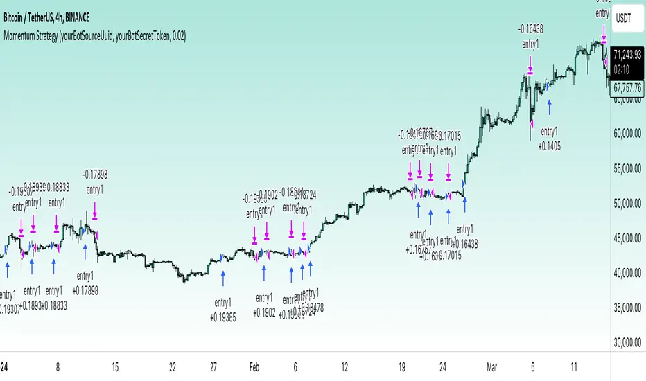
AI Momentum [YinYang]Overview:
AI Momentum is a kernel function based momentum Indicator. It uses Rational Quadratics to help smooth out the Moving Averages, this may give them a more accurate result. This Indicator has 2 main uses, first it displays ‘Zones’ that help you visualize the potential movement areas and when the price is out of bounds (Overvalued or Undervalued). Secondly it creates signals that display the momentum of the current trend.
The Zones are composed of the Highest Highs and Lowest lows turned into a Rational Quadratic over varying lengths. These create our Rational High and Low zones. There is however a second zone. The second zone is composed of the avg of the Inner High and Inner Low zones (yellow line) and the Rational Quadratic of the current Close. This helps to create a second zone that is within the High and Low bounds that may represent momentum changes within these zones. When the Rationalized Close crosses above the High and Low Zone Average it may signify a bullish momentum change and vice versa when it crosses below.
There are 3 different signals created to display momentum:
Bullish and Bearish Momentum. These signals display when there is current bullish or bearish momentum happening within the trend. When the momentum changes there will likely be a lull where there are neither Bullish or Bearish momentum signals. These signals may be useful to help visualize when the momentum has started and stopped for both the bulls and the bears. Bullish Momentum is calculated by checking if the Rational Quadratic Close > Rational Quadratic of the Highest OHLC4 smoothed over a VWMA. The Bearish Momentum is calculated by checking the opposite.
Overly Bullish and Bearish Momentum. These signals occur when the bar has Bullish or Bearish Momentum and also has an Rationalized RSI greater or less than a certain level. Bullish is >= 57 and Bearish is <= 43. There is also the option to ‘Factor Volume’ into these signals. This means, the Overly Bullish and Bearish Signals will only occur when the Rationalized Volume > VWMA Rationalized Volume as well as the previously mentioned factors above. This can be useful for removing ‘clutter’ as volume may dictate when these momentum changes will occur, but it can also remove some of the useful signals and you may miss the swing too if the volume just was low. Overly Bullish and Bearish Momentum may dictate when a momentum change will occur. Remember, they are OVERLY Bullish and Bearish, meaning there is a chance a correction may occur around these signals.
Bull and Bear Crosses. These signals occur when the Rationalized Close crosses the Gaussian Close that is 2 bars back. These signals may show when there is a strong change in momentum, but be careful as more often than not they’re predicting that the momentum may change in the opposite direction.
Tutorial:
As we can see in the example above, generally what happens is we get the regular Bullish or Bearish momentum, followed by the Rationalized Close crossing the Zone average and finally the Overly Bullish or Bearish signals. This is normally the order of operations but isn’t always how it happens as sometimes momentum changes don’t make it that far; also the Rationalized Close and Zone Average don’t follow any of the same math as the Signals which can result in differing appearances. The Bull and Bear Crosses are also quite sporadic in appearance and don’t generally follow any sort of order of operations. However, they may occur as a Predictor between Bullish and Bearish momentum, signifying the beginning of the momentum change.
The Bull and Bear crosses may be a Predictor of momentum change. They generally happen when there is no Bullish or Bearish momentum happening; and this helps to add strength to their prediction. When they occur during momentum (orange circle) there is a less likely chance that it will happen, and may instead signify the exact opposite; it may help predict a large spike in momentum in the direction of the Bullish or Bearish momentum. In the case of the orange circle, there is currently Bearish Momentum and therefore the Bull Cross may help predict a large momentum movement is about to occur in favor of the Bears.
We have disabled signals here to properly display and talk about the zones. As you can see, Rationalizing the Highest Highs and Lowest Lows over 2 different lengths creates inner and outer bounds that help to predict where parabolic movement and momentum may move to. Our Inner and Outer zones are great for seeing potential Support and Resistance locations.
The secondary zone, which can cross over and change from Green to Red is also a very important zone. Let's zoom in and talk about it specifically.
The Middle Zone Crosses may help deduce where parabolic movement and strong momentum changes may occur. Generally what may happen is when the cross occurs, you will see parabolic movement to the High / Low zones. This may be the Inner zone but can sometimes be the outer zone too. The hard part is sometimes it can be a Fakeout, like displayed with the Blue Circle. The Cross doesn’t mean it may move to the opposing side, sometimes it may just be predicting Parabolic movement in a general sense.
When we turn the Momentum Signals back on, we can see where the Fakeout occurred that it not only almost hit the Inner Low Zone but it also exhibited 2 Overly Bearish Signals. Remember, Overly bearish signals mean a momentum change in favor of the Bulls may occur soon and overly Bullish signals mean a momentum change in favor of the Bears may occur soon.
You may be wondering, well what does “may occur soon” mean and how do we tell?
The purpose of the momentum signals is not only to let you know when Momentum has occurred and when it is still prevalent. It also matters A LOT when it has STOPPED!
In this example above, we look at when the Overly Bullish and Bearish Momentum has STOPPED. As you can see, when the Overly Bullish or Bearish Momentum stopped may be a strong predictor of potential momentum change in the opposing direction.
We will conclude our Tutorial here, hopefully this Indicator has been helpful for showing you where momentum is occurring and help predict how far it may move. We have been dabbling with and are planning on releasing a Strategy based on this Indicator shortly.
Settings:
1. Momentum:
Show Signals: Sometimes it can be difficult to visualize the zones with signals enabled.
Factor Volume: Factor Volume only applies to Overly Bullish and Bearish Signals. It's when the Volume is > VWMA Volume over the Smoothing Length.
Zone Inside Length: The Zone Inside is the Inner zone of the High and Low. This is the length used to create it.
Zone Outside Length: The Zone Outside is the Outer zone of the High and Low. This is the length used to create it.
Smoothing length: Smoothing length is the length used to smooth out our Bullish and Bearish signals, along with our Overly Bullish and Overly Bearish Signals.
2. Kernel Settings:
Lookback Window: The number of bars used for the estimation. This is a sliding value that represents the most recent historical bars. Recommended range: 3-50.
Relative Weighting: Relative weighting of time frames. As this value approaches zero, the longer time frames will exert more influence on the estimation. As this value approaches infinity, the behavior of the Rational Quadratic Kernel will become identical to the Gaussian kernel. Recommended range: 0.25-25.
Start Regression at Bar: Bar index on which to start regression. The first bars of a chart are often highly volatile, and omission of these initial bars often leads to a better overall fit. Recommended range: 5-25.
If you have any questions, comments, ideas or concerns please don't hesitate to contact us.
HAPPY TRADING!
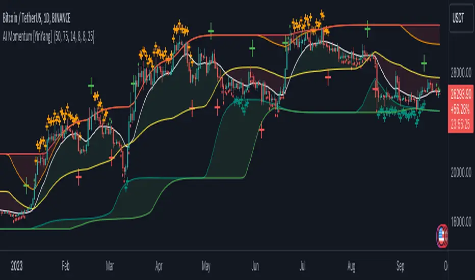
Value At RiskThe Value at Risk Channel (VaR Channel) is a trading indicator designed to assist traders in managing their risk exposure effectively. By allowing users to select a specific time period and a probability value, this indicator generates upper and lower limits that the price might potentially attain within the chosen timeframe and probability range.
CONCEPTS
This indicator employs the concept of Value at Risk (VaR) calculation, a crucial metric in risk management. VaR quantifies the potential financial loss within a position, portfolio, or company over a defined time period. Financial institutions like banks and investment firms use VaR to estimate the extent and likelihood of potential losses in their portfolios.
The "historical method" is utilized to compute VaR within the indicator. This method analyzes the historical performance of returns and constructs a histogram representing the statistical distribution of past returns. Assuming returns adhere to a normal distribution, probabilities are assigned to different return values based on their position in the distribution percentile.
HOW TO USE
Suppose you wish to plot upper and lower price limits for a 4-hour period with a 5% probability. Access the indicator's Settings tab and set the Timeframe parameter to "4 hours" while configuring the Probability parameter to 5.0.
The indicator serves as a tool to determine appropriate Stop-Loss levels triggering with low probability. Additionally, it helps gauge the likelihood of triggering such levels.
Likewise, you can assess the probability of your desired Take-Profit level being reached within a specified time frame. For instance, if you anticipate your target to be achieved within a week, set the Timeframe parameter to "1 week" and adjust the Probability parameter to align the VaR channel's limits with your Take-Profit level. The resulting Probability parameter value reflects the likelihood of your target being met within the expected time frame.
This indicator proves valuable for evaluating and managing risk, as well as refining trading strategies. If you discover other applications for this indicator, feel free to share them in the comments!
SETTINGS
Timeframe: Designates the time period within which the price might touch the VaR channel's upper or lower boundary, considering the specified Probability parameter.
Probability: Defines the likelihood of the price reaching the VaR channel's upper or lower limit during the timeframe determined by the Timeframe parameter.
Window: Establishes the historical period (number of past bars) utilized for VaR calculation.

Fair value bands / quantifytools— Overview
Fair value bands, like other band tools, depict dynamic points in price where price behaviour is normal or abnormal, i.e. trading at/around mean (price at fair value) or deviating from mean (price outside fair value). Unlike constantly readjusting standard deviation based bands, fair value bands are designed to be smooth and constant, based on typical historical deviations. The script calculates pivots that take place above/below fair value basis and forms median deviation bands based on this information. These points are then multiplied up to 3, representing more extreme deviations.
By default, the script uses OHLC4 and SMA 20 as basis for the bands. Users can form their preferred fair value basis using following options:
Price source
- Standard OHLC values
- HL2 (High + low / 2)
- OHLC4 (Open + high + low + close / 4)
- HLC3 (High + low + close / 3)
- HLCC4 (High + low + close + close / 4)
Smoothing
- SMA
- EMA
- HMA
- RMA
- WMA
- VWMA
- Median
Once fair value basis is established, some additional customization options can be employed:
Trend mode
Direction based
Cross based
Trend modes affect fair value basis color that indicates trend direction. Direction based trend considers only the direction of the defined fair value basis, i.e. pointing up is considered an uptrend, vice versa for downtrend. Cross based trends activate when selected source (same options as price source) crosses fair value basis. These sources can be set individually for uptrend/downtrend cross conditions. By default, the script uses cross based trend mode with low and high as sources.
Cross based (downtrend not triggered) vs. direction based (downtrend triggered):
Threshold band
Threshold band is calculated using typical deviations when price is trading at fair value basis. In other words, a little bit of "wiggle room" is added around the mean based on expected deviation. This feature is useful for cross based trends, as it allows filtering insignificant crosses that are more likely just noise. By default, threshold band is calculated based on 1x median deviation from mean. Users can increase/decrease threshold band width via input menu for more/less noise filtering, e.g. 2x threshold band width would require price to cross wiggle room that is 2x wider than typical, 0x erases threshold band altogether.
Deviation bands
Width of deviation bands by default is based on 1x median deviations and can be increased/decreased in a similar manner to threshold bands.
Each combination of customization options produces varying behaviour in the bands. To measure the behaviour and finding fairest representation of fair and unfair value, some data is gathered.
— Fair value metrics
Space between each band is considered a lot, named +3, +2, +1, -1, -2, -3. For each lot, time spent and volume relative to volume moving average (SMA 20) is recorded each time price is trading in a given lot:
Depending on the asset, timeframe and chosen fair value basis, shape of the distributions vary. However, practically always time is distributed in a normal bell curve shape, being highest at lots +1 to -1, gradually decreasing the further price is from the mean. This is hardly surprising, but it allows accurately determining dynamic areas of normal and abnormal price behaviour (i.e. low risk area between +1 and -1, high risk area between +-2 to +-3). Volume on the other hand is typically distributed the other way around, being lowest at lots +1 to -1 and highest at +-2 to +-3. When time and volume are distributed like so, we can conclude that 1) price being outside fair value is a rare event and 2) the more price is outside fair value, the more anomaly behaviour in volume we tend to find.
Viewing metric calculations
Metric calculation highlights can be enabled from the input menu, resulting in a lot based coloring and visibility of each lot counter (time, cumulative relative volume and average relative volume) in data window:
— Alerts
Available alerts are the following:
Individual
- High crossing deviation band (bands +1 to +3 )
- Low crossing deviation band (bands -1 to -3 )
- Low at threshold band in an uptrend
- High at threshold band in a downtrend
- New uptrend
- New downtrend
Grouped
- New uptrend or downtrend
- Deviation band cross (+1 or -1)
- Deviation band cross (+2 or -2)
- Deviation band cross (+3 or -3)
— Practical guide
Example #1 : Risk on/risk off trend following
Ideal trend stays inside fair value and provides sufficient cool offs between the moves. When this is the case, fair value bands can be used for sensible entry/exit levels within the trend.
Example #2 : Mean reversions
When price shows exuberance into an extreme deviation, followed by a stall and signs of exhaustion (wicks), an opportunity for mean reversion emerges. The higher the deviation, the more volatility in the move, the more signalling of exhaustion, the better.
Example #3 : Tweaking bands for desired behaviour
The faster the length of fair value basis, the more momentum price needs to hit extreme deviation levels, as bands too are moving faster alongside price. Decreasing fair value basis length typically leads to more quick and aggressive deviations and less steady trends outside fair value.

base16Library "base16"
Base16 Syntax Theme Collection. dark/light Pairs placed into 2 matched groups.
included is tool for assembling your own themes, as well as all themes String names
to create your own Input menus / add to your own theme matrix, and theme selectors
addToMatrix(_mtx, _title, _choices, _theme)
To create a theme matrix with string index, use a color matrix global
add theme name to string array of theme titles
and last input a theme from above, or create your own theme arrays.
Parameters:
_mtx : (color ) matrix for storage
_title : (string ) Name of theme being added
_choices : (string ) name index
_theme : (color ) colors being added
Returns: void
addToMatrix(_mtx, _theme)
Add theme to color matrix Non-indexed
Parameters:
_mtx : (color ) matrix for storage
_theme : (color ) colors being added
dark()
Dark Themne Selection (With light Equivalent in same location)
Returns: Color matrix of dark themes
light()
light Themne Selection (With dark Equivalent in same location)
Returns: Color matrix of light themes
selectTheme(_mtx, _themes, _theme)
Get a Theme By Name
Parameters:
_mtx : (Matrix color) Name of Theme
_themes : (Array string) Array with Names of Themes
_theme : (string ) Name of Theme to select
selectTheme(_mtx, _theme)
Get a Theme By Number
Parameters:
_mtx : (Matrix color) Name of Theme
_theme : (int ) Number of Theme to select
/// all themes included:
3024
apathy
apprentice
ashes
atelier_cave_light
atelier_cave
atelier_dune_light
atelier_dune
atelier_estuary_light
atelier_estuary
atelier_forest_light
atelier_forest
atelier_heath_light
atelier_heath
atelier_lakeside_light
atelier_lakeside
atelier_plateau_light
atelier_plateau
atelier_savanna_light
atelier_savanna
atelier_seaside_light
atelier_seaside
atelier_sulphurpool_light
atelier_sulphurpool
atlas
ayu_dark
ayu_light
ayu_mirage
bespin
black_metal_bathory
black_metal_burzum
black_metal_dark_funeral
black_metal_gorgoroth
black_metal_immortal
black_metal_khold
black_metal_marduk
black_metal_mayhem
black_metal_nile
black_metal_venom
black_metal
blue_forest
blueish
brewer
bright
brogrammer
brush_trees_dark
brush_trees
catppuccin
chalk
circus
classic_dark
classic_light
codeschool
clrs
cupcake
cupertino
da_one_black
da_one_gray
da_one_ocean
da_one_paper
da_one_sea
da_one_white
danqing_light
danqing
darcula
darkmoss
darktooth
dark_violet
decaf
default_dark
default_light
dirtysea
dracula
edge_dark
edge_light
eighties
embers
emil
equilibrium_dark
equilibrium_gray_dark
equilibrium_gray_light
equilibrium_light
espresso
eva_dim
eva
everforest
flat
framer
fruit_soda
gigavolt
github
google_dark
google_light
gotham
grayscale_dark
grayscale_light
green_screen
gruber
gruvbox_dark_hard
gruvbox_dark_medium
gruvbox_dark_pale
gruvbox_dark_soft
gruvbox_light_hard
gruvbox_light_medium
gruvbox_light_soft
gruvbox_material_dark_hard
gruvbox_material_dark_medium
gruvbox_material_dark_soft
gruvbox_material_light_hard
gruvbox_material_light_medium
gruvbox_material_light_soft
hardcore
harmonic16_dark
harmonic16_light
heetch_light
heetch_dark
helios
hopscotch
horizon_dark
horizon_light
horizon_terminal_dark
horizon_terminal_light
humanoid_dark
humanoid_light
ia_dark
ia_light
icy_dark
ir_black
isotope
kanagawa
katy
kimber
lime
macintosh
marrakesh
materia
material_darker
material_lighter
material_palenight
material_vivid
material
mellow_purple
mexico_light
mocha
monokai
Nebula
nord
nova
ocean
oceanicnext
one_light
onedark
outrun_dark
pandora
papercolor_dark
papercolor_light
paraiso
pasque
phd
pico
pinky
pop
porple
primer_dark_dimmed
primer_dark
primer_light
purpledream
qualia
railscasts
rebecca
rose_pine_dawn
rose_pine_moon
rose_pine
sagelight
sakura
sandcastle
seti_ui
shades_of_purple
shadesmear_dark
shadesmear_light
shapeshifter
silk_dark
silk_light
snazzy
solar_flare_light
solar_flare
solarized_dark
solarized_light
spaceduck
spacemacs
stella
still_alive
summercamp
summerfruit_dark
summerfruit_light
synth_midnight_terminal_dark
synth_midnight_terminal_light
tango
tender
tokyo_city_dark
tokyo_city_light
tokyo_city_terminal_dark
tokyo_city_terminal_light
tokyo_night_dark
tokyo_night_light
tokyo_night_storm
tokyo_night_terminal_dark
tokyo_night_terminal_light
tokyo_night_terminal_storm
tokyodark_terminal
tokyodark
tomorrow_night_eighties
tomorrow_night
tomorrow
london_tube
twilight
unikitty_dark
unikitty_light
unikitty_reversible
uwunicorn
vice
vulcan
windows_10_light
windows_10
windows_95_light
windows_95
windows_high_contrast_light
windows_high_contrast
windows_nt_light
windows_nt
woodland
xcode_dusk
zenburn
