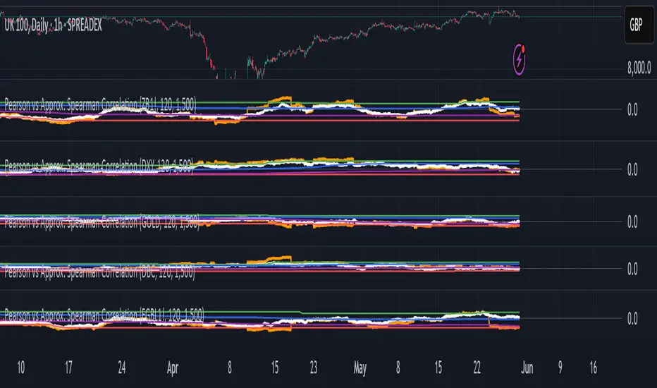
Pearson vs Approx. Spearman CorrelationThis indicator displays the rolling Pearson and approximate Spearman correlation between the chart's asset and a second user-defined asset, based on log returns over a customizable window.
Features:
- Pearson correlation of log returns (standard linear dependency measure)
- Approximate Spearman correlation, using percentile ranks to better capture nonlinear and monotonic relationships
/ Horizontal lines showing:
Maximum and minimum correlation values over a statistical window
1st quartile (25%) and 3rd quartile (75%) — helpful for identifying statistically high or low regimes
This script is useful for identifying dynamic co-movements, regime changes, or correlation breakdowns between assets — applicable in risk management, portfolio construction, and pairs trading strategies.
Cerca negli script per "如何用wind搜索股票的发行价和份数"
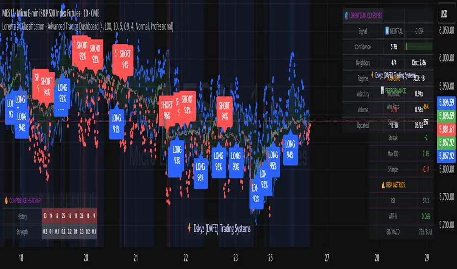
Lorentzian Classification - Advanced Trading DashboardLorentzian Classification - Relativistic Market Analysis
A Journey from Theory to Trading Reality
What began as fascination with Einstein's relativity and Lorentzian geometry has evolved into a practical trading tool that bridges theoretical physics and market dynamics. This indicator represents months of wrestling with complex mathematical concepts, debugging intricate algorithms, and transforming abstract theory into actionable trading signals.
The Theoretical Foundation
Lorentzian Distance in Market Space
Traditional Euclidean distance treats all feature differences equally, but markets don't behave uniformly. Lorentzian distance, borrowed from spacetime geometry, provides a more nuanced similarity measure:
d(x,y) = Σ ln(1 + |xi - yi|)
This logarithmic formulation naturally handles:
Scale invariance: Large price moves don't overwhelm small but significant patterns
Outlier robustness: Extreme values are dampened rather than dominating
Non-linear relationships: Captures market behavior better than linear metrics
K-Nearest Neighbors with Relativistic Weighting
The algorithm searches historical market states for patterns similar to current conditions. Each neighbor receives weight inversely proportional to its Lorentzian distance:
w = 1 / (1 + distance)
This creates a "gravitational" effect where closer patterns have stronger influence on predictions.
The Implementation Challenge
Creating meaningful market features required extensive experimentation:
Price Features: Multi-timeframe momentum (1, 2, 3, 5, 8 bar lookbacks) Volume Features: Relative volume analysis against 20-period average
Volatility Features: ATR and Bollinger Band width normalization Momentum Features: RSI deviation from neutral and MACD/price ratio
Each feature undergoes min-max normalization to ensure equal weighting in distance calculations.
The Prediction Mechanism
For each current market state:
Feature Vector Construction: 12-dimensional representation of market conditions
Historical Search: Scan lookback period for similar patterns using Lorentzian distance
Neighbor Selection: Identify K nearest historical matches
Outcome Analysis: Examine what happened N bars after each match
Weighted Prediction: Combine outcomes using distance-based weights
Confidence Calculation: Measure agreement between neighbors
Technical Hurdles Overcome
Array Management: Complex indexing to prevent look-ahead bias
Distance Calculations: Optimizing nested loops for performance
Memory Constraints: Balancing lookback depth with computational limits
Signal Filtering: Preventing clustering of identical signals
Advanced Dashboard System
Main Control Panel
The primary dashboard provides real-time market intelligence:
Signal Status: Current prediction with confidence percentage
Neighbor Analysis: How many historical patterns match current conditions
Market Regime: Trend strength, volatility, and volume analysis
Temporal Context: Real-time updates with timestamp
Performance Analytics
Comprehensive tracking system monitors:
Win Rate: Percentage of successful predictions
Signal Count: Total predictions generated
Streak Analysis: Current winning/losing sequence
Drawdown Monitoring: Maximum equity decline
Sharpe Approximation: Risk-adjusted performance estimate
Risk Assessment Panel
Multi-dimensional risk analysis:
RSI Positioning: Overbought/oversold conditions
ATR Percentage: Current volatility relative to price
Bollinger Position: Price location within volatility bands
MACD Alignment: Momentum confirmation
Confidence Heatmap
Visual representation of prediction reliability:
Historical Confidence: Last 10 periods of prediction certainty
Strength Analysis: Magnitude of prediction values over time
Pattern Recognition: Color-coded confidence levels for quick assessment
Input Parameters Deep Dive
Core Algorithm Settings
K Nearest Neighbors (1-20): More neighbors create smoother but less responsive signals. Optimal range 5-8 for most markets.
Historical Lookback (50-500): Deeper history improves pattern recognition but reduces adaptability. 100-200 bars optimal for most timeframes.
Feature Window (5-30): Longer windows capture more context but reduce sensitivity. Match to your trading timeframe.
Feature Selection
Price Changes: Essential for momentum and reversal detection Volume Profile: Critical for institutional activity recognition Volatility Measures: Key for regime change detection Momentum Indicators: Vital for trend confirmation
Signal Generation
Prediction Horizon (1-20): How far ahead to predict. Shorter horizons for scalping, longer for swing trading.
Signal Threshold (0.5-0.9): Confidence required for signal generation. Higher values reduce false signals but may miss opportunities.
Smoothing (1-10): EMA applied to raw predictions. More smoothing reduces noise but increases lag.
Visual Design Philosophy
Color Themes
Professional: Corporate blue/red for institutional environments Neon: Cyberpunk cyan/magenta for modern aesthetics
Matrix: Green/red hacker-inspired palette Classic: Traditional trading colors
Information Hierarchy
The dashboard system prioritizes information by importance:
Primary Signals: Largest, most prominent display
Confidence Metrics: Secondary but clearly visible
Supporting Data: Detailed but unobtrusive
Historical Context: Available but not distracting
Trading Applications
Signal Interpretation
Long Signals: Prediction > threshold with high confidence
Look for volume confirmation
- Check trend alignment
- Verify support levels
Short Signals: Prediction < -threshold with high confidence
Confirm with resistance levels
- Check for distribution patterns
- Verify momentum divergence
- Market Regime Adaptation
Trending Markets: Higher confidence in directional signals
Ranging Markets: Focus on reversal signals at extremes
Volatile Markets: Require higher confidence thresholds
Low Volume: Reduce position sizes, increase caution
Risk Management Integration
Confidence-Based Sizing: Larger positions for higher confidence signals
Regime-Aware Stops: Wider stops in volatile regimes
Multi-Timeframe Confirmation: Align signals across timeframes
Volume Confirmation: Require volume support for major signals
Originality and Innovation
This indicator represents genuine innovation in several areas:
Mathematical Approach
First application of Lorentzian geometry to market pattern recognition. Unlike Euclidean-based systems, this naturally handles market non-linearities.
Feature Engineering
Sophisticated multi-dimensional feature space combining price, volume, volatility, and momentum in normalized form.
Visualization System
Professional-grade dashboard system providing comprehensive market intelligence in intuitive format.
Performance Tracking
Real-time performance analytics typically found only in institutional trading systems.
Development Journey
Creating this indicator involved overcoming numerous technical challenges:
Mathematical Complexity: Translating theoretical concepts into practical code
Performance Optimization: Balancing accuracy with computational efficiency
User Interface Design: Making complex data accessible and actionable
Signal Quality: Filtering noise while maintaining responsiveness
The result is a tool that brings institutional-grade analytics to individual traders while maintaining the theoretical rigor of its mathematical foundation.
Best Practices
- Parameter Optimization
- Start with default settings and adjust based on:
Market Characteristics: Volatile vs. stable
Trading Timeframe: Scalping vs. swing trading
Risk Tolerance: Conservative vs. aggressive
Signal Confirmation
Never trade on Lorentzian signals alone:
Price Action: Confirm with support/resistance
Volume: Verify with volume analysis
Multiple Timeframes: Check higher timeframe alignment
Market Context: Consider overall market conditions
Risk Management
Position Sizing: Scale with confidence levels
Stop Losses: Adapt to market volatility
Profit Targets: Based on historical performance
Maximum Risk: Never exceed 2-3% per trade
Disclaimer
This indicator is for educational and research purposes only. It does not constitute financial advice or guarantee profitable trading results. The Lorentzian classification system reveals market patterns but cannot predict future price movements with certainty. Always use proper risk management, conduct your own analysis, and never risk more than you can afford to lose.
Market dynamics are inherently uncertain, and past performance does not guarantee future results. This tool should be used as part of a comprehensive trading strategy, not as a standalone solution.
Bringing the elegance of relativistic geometry to market analysis through sophisticated pattern recognition and intuitive visualization.
Thank you for sharing the idea. You're more than a follower, you're a leader!
@vasanthgautham1221
Trade with precision. Trade with insight.
— Dskyz , for DAFE Trading Systems
Multi-Session ORBThe Multi-Session ORB Indicator is a customizable Pine Script (version 6) tool designed for TradingView to plot Opening Range Breakout (ORB) levels across four major trading sessions: Sydney, Tokyo, London, and New York. It allows traders to define specific ORB durations and session times in Central Daylight Time (CDT), making it adaptable to various trading strategies.
Key Features:
1. Customizable ORB Duration: Users can set the ORB duration (default: 15 minutes) via the inputMax parameter, determining the time window for calculating the high and low of each session’s opening range.
2. Flexible Session Times: The indicator supports user-defined session and ORB times for:
◦ Sydney: Default ORB (17:00–17:15 CDT), Session (17:00–01:00 CDT)
◦ Tokyo: Default ORB (19:00–19:15 CDT), Session (19:00–04:00 CDT)
◦ London: Default ORB (02:00–02:15 CDT), Session (02:00–11:00 CDT)
◦ New York: Default ORB (08:30–08:45 CDT), Session (08:30–16:00 CDT)
3. Session-Specific ORB Levels: For each session, the indicator calculates and tracks the high and low prices during the specified ORB period. These levels are updated dynamically if new highs or lows occur within the ORB timeframe.
4. Visual Representation:
◦ ORB high and low lines are plotted only during their respective session times, ensuring clarity.
◦ Each session’s lines are color-coded for easy identification:
▪ Sydney: Light Yellow (high), Dark Yellow (low)
▪ Tokyo: Light Pink (high), Dark Pink (low)
▪ London: Light Blue (high), Dark Blue (low)
▪ New York: Light Purple (high), Dark Purple (low)
◦ Lines are drawn with a linewidth of 2 and disappear when the session ends or if the timeframe is not intraday (or exceeds the ORB duration).
5. Intraday Compatibility: The indicator is optimized for intraday timeframes (e.g., 1-minute to 15-minute charts) and only displays when the chart’s timeframe multiplier is less than or equal to the ORB duration.
How It Works:
• Session Detection: The script uses the time() function to check if the current bar falls within the user-defined ORB or session time windows, accounting for all days of the week.
• ORB Logic: At the start of each session’s ORB period, the script initializes the high and low based on the first bar’s prices. It then updates these levels if subsequent bars within the ORB period exceed the current high or fall below the current low.
• Plotting: ORB levels are plotted as horizontal lines during the respective session, with visibility controlled to avoid clutter outside session times or on incompatible timeframes.
Use Case:
Traders can use this indicator to identify key breakout levels for each trading session, facilitating strategies based on price action around the opening range. The flexibility to adjust ORB and session times makes it suitable for various markets (e.g., forex, stocks, or futures) and time zones.
Limitations:
• The indicator is designed for intraday timeframes and may not display on higher timeframes (e.g., daily or weekly) or if the timeframe multiplier exceeds the ORB duration.
• Time inputs are in CDT, requiring users to adjust for their local timezone or market requirements.
• If you need to use this for GC/CL/SPY/QQQ you have to adjust the times by one hour.
This indicator is ideal for traders focusing on session-based breakout strategies, offering clear visualization and customization for global market sessions.

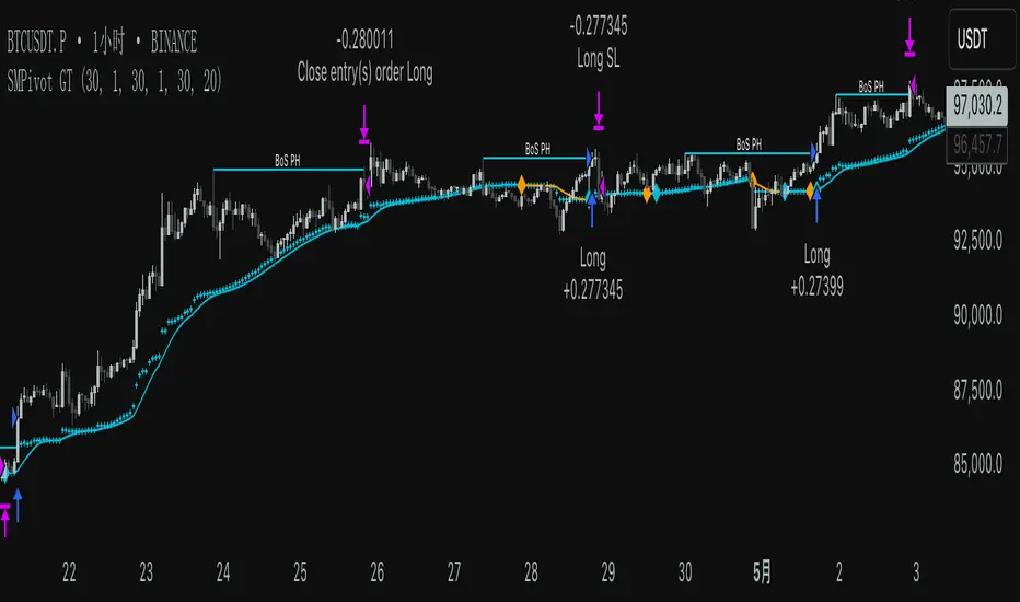
SMPivot Gaussian Trend Strategy [Js.K]This open-source strategy combines a Gaussian-weighted moving average with “Smart Money” swing-pivot breaks (BoS = Break-of-Structure) to capture trend continuations and early reversals. It is intended for educational and research purposes only and must not be interpreted as financial advice.
How the logic works
-------------------
1. Gaussian Moving Average (GMA)
• A custom Gaussian kernel (length = 30 by default) smooths price while preserving turning points.
• A second pass (“Smoothed GMA”) further filters noise; only its direction is used for bias.
2. Swing-Pivot detection
• High/Low pivots are found with a symmetric look-back/forward window (Pivot Length = 20).
• The most recent confirmed pivot creates a dynamic structure level (UpdatedHigh / UpdatedLow).
3. Entry rules
Long
• Price closes above the most recent pivot high **and** above Smoothed GMA.
Short
• Price closes below the most recent pivot low **and** below Smoothed GMA.
4. Exit rules
• Fixed stop-loss and take-profit in percent of current price (user-defined).
• Separate parameters and on/off switches for longs and shorts.
5. Visuals
• GMA (dots) and Smoothed GMA (line).
• Structure break lines plus “BoS PH/PL” labels at the midpoint between pivot and break.
Inputs
------
Gaussian
• Gaussian Length (default 30) – smoothing window.
• Gaussian Scatterplot – toggle GMA dots.
Smart-Money Pivot
• Pivot Length (default 20).
• Bull / Bear colors.
Risk settings
• Long / Short enable.
• Individual SL % and TP % (default 1 % SL, 30 % TP).
• Strategy uses percent-of-equity sizing; initial capital defaults to 10 000 USD.
Adjust these to reflect your own account size, realistic commission and slippage.
Best practice & compliance notes
--------------------------------
• Test on a data sample that yields ≥ 100 trades to obtain statistically relevant results.
• Keep risk per trade below 5–10 % of equity; the default values comply with this guideline.
• Explain any custom settings you publish that differ from the defaults.
• Do **not** remove the code header or licence notice (MPL-2.0).
• Include realistic commission and slippage in your back-test before publishing.
• The script does **not** repaint; orders are processed on bar close.
Usage
-----
1. Add the script to any symbol / timeframe; intraday and swing timeframes both work—adjust lengths accordingly.
2. Configure SL/TP and position size to match your personal risk management.
3. Run “List of trades” and the performance summary to evaluate expectancy; forward-test before live use.
Disclaimer
----------
Trading involves substantial risk. Past performance based on back-testing is not necessarily indicative of future results. The author is **not** responsible for any financial losses arising from the use of this script.
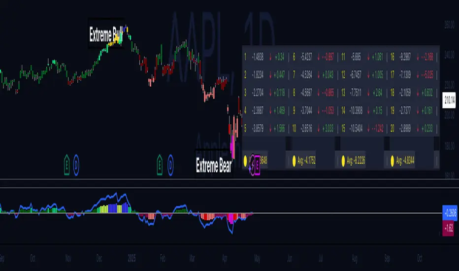
Hippo Battlefield - Bulls VS Bears 20 bars## Hippo Battlefield – Bulls VS Bears (20 Bars)
**What it is**
A multi-dimensional momentum-and-sentiment oscillator that combines classic Bull/Bear Power with ATR- or peak-normalization, then layers on RSI and MACD-derived metrics into:
1. **A colored bar series** showing net Bull+Bear Power strength over the last 20 bars,
2. **A dynamic table** of each of those 20 BBP values (grouped into four 5-bar “quartals”), with symbols, per-bar change, and rolling averages, and
3. **A composite “Weighted BBP” histogram** blending normalized RSI, MACD, and BBP into a single view.
---
### Key Inputs
- **Length (EMA)** – look-back for the underlying EMA (default 60)
- **Normalization Length** – look-back window for peak-normalization (default 60)
- **Use ATR for Norm.** – toggle ATR-based normalization vs. highest-abs(BBP)
- **Show Tables** – toggle the bottom-right 21×11 grid of raw and average BBP values
---
### What You See
#### 1. Colored Bars (Overlay = false)
- Bars are colored by normalized BBP intensity:
- Extreme Bull (≥+10): deep blue
- Strong Bull (+5 to +10): green/yellow
- Weak Bull (+0 to +5): dark green
- Weak Bear (–0 to –5): dark red
- Strong Bear (–5 to –10): pink/red
- Extreme Bear (<–10): magenta
#### 2. Bottom-Right Table (20 Bars of Data)
- Divided into four columns (0–4, 5–9, 10–14, 15–19 bars ago) and one “average” row.
- Each cell shows:
1. Bar index (1–20),
2. Normalized BBP value (to four decimals),
3. Direction symbol (↑/↓/=),
4. Bar-to-bar change (± value),
5. A separator “|”.
- At the very bottom, each column’s 5-bar average is displayed as “Avg: X.XXXX” with a dot marker.
#### 3. Top-Center Mini-Table
- When ≥20 bars have elapsed, shows the date at 20 bars ago and the average BBP across the full 20-bar window.
#### 4. Normalized RSI Line
- Rescales the classic 14-period RSI into a –20…+20 band to align with BBP.
#### 5. MACD Lines (Hidden) & Composite Histogram
- MACD and signal lines are calculated but not plotted by default.
- A “Weighted BBP” histogram combines:
- 20% normalized RSI,
- 20% average of (MACD + signal + normalized BBP),
- 60% normalized BBP
- Plotted as columns, color-coded by strength using the same palette as the main bars.
#### 6. Middle Reference Line
- A horizontal zero line to anchor over/under-zero readings.
---
### How to Use It
- **Trend confirmation**: Strong blue/green bars alongside a rising histogram suggest bull conviction; strong reds/magentas signal bear dominance.
- **Divergence spotting**: Watch for price making new highs/lows while BBP or the histogram fails to follow.
- **Quartal analysis**: The 5-bar group averages can reveal whether recent momentum is accelerating or waning.
- **Cross-indicator weighting**: Because RSI, MACD, and raw BBP all feed into the final histogram, you get a smoothed, blended view of momentum shifts.
---
**Tip:** Tweak the EMA and normalization length to suit your preferred timeframe (e.g. shorter for intraday scalps, longer for swing trades). Enable/disable the table if you prefer a cleaner pane.
Aggregate PDH High Break Alert**Aggregate PDH High Break Alert**
**Overview**
The “Aggregate PDH High Break Alert” is a lightweight Pine Script v6 indicator designed to instantly notify you when today’s price breaks above any prior-day high in a user-defined lookback window. Instead of manually scanning dozens of daily highs, this script automatically loops through the last _N_ days (up to 100) and fires a single-bar alert the moment price eclipses a specific day’s high.
**Key Features**
- **Dynamic Lookback**: Choose any lookback period from 1 to 100 days via a single `High-Break Lookback` input.
- **Single Security Call**: Efficiently retrieves the entire daily-high series in one call to avoid TradingView’s 40-call security limit.
- **Automatic Looping**: Internally loops through each prior-day high, so there’s no need to manually code dozens of lines.
- **Custom Alerts**: Generates a clear, formatted alert message—e.g. “Crossed high from 7 day(s) ago”—for each breakout.
- **Lightweight & Maintainable**: Compact codebase (<15 lines) makes tweaking and debugging a breeze.
**Inputs**
- **High-Break Lookback (days)**: Number of past days to monitor for high breaks. Valid range: 1–100.
**How to Use**
1. **Add to Chart**: Open TradingView, click “Indicators,” then “Create,” and paste in the code.
2. **Configure Lookback**: In the script’s settings, set your desired lookback window (e.g., 20 for the past 20 days).
3. **Enable Alerts**: Right-click the indicator’s name on your chart, select “Add Alert on Aggregate PDH High Break Alert,” and choose “Once per bar close.”
4. **Receive Notifications**: Whenever price crosses above any of the specified prior-day highs, you’ll get an on-screen and/or mobile push alert with the exact number of days ago.
**Use Cases**
- **Trend Confirmation**: Confirm fresh bullish momentum when today’s high outpaces any of the last _N_ days.
- **Breakout Trading**: Automate entries off multi-day highs without manual chart scanning.
- **System Integration**: Integrate with alerts to trigger orders in third-party bots or webhook receivers.
**Disclaimer**
Breakouts alone do not guarantee sustained moves. Combine with your preferred risk management, volume filters, and other indicators for higher-probability setups. Use on markets and timeframes where daily breakout behavior aligns with your strategy.

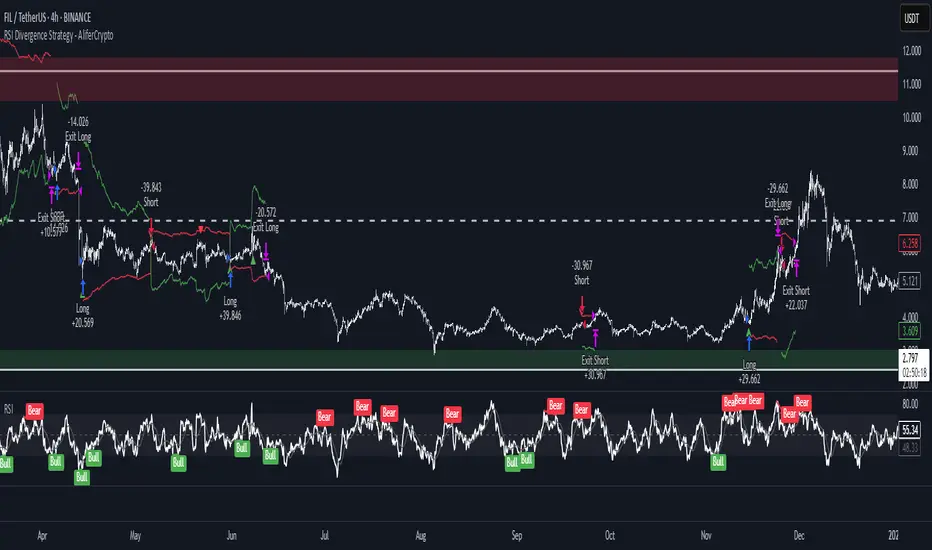
RSI Divergence Strategy - AliferCryptoStrategy Overview
The RSI Divergence Strategy is designed to identify potential reversals by detecting regular bullish and bearish divergences between price action and the Relative Strength Index (RSI). It automatically enters positions when a divergence is confirmed and manages risk with configurable stop-loss and take-profit levels.
Key Features
Automatic Divergence Detection: Scans for RSI pivot lows/highs vs. price pivots using user-defined lookback windows and bar ranges.
Dual SL/TP Methods:
- Swing-based: Stops placed a configurable percentage beyond the most recent swing high/low.
- ATR-based: Stops placed at a multiple of Average True Range, with a separate risk/reward multiplier.
Long and Short Entries: Buys on bullish divergences; sells short on bearish divergences.
Fully Customizable: Input groups for RSI, divergence, swing, ATR, and general SL/TP settings.
Visual Plotting: Marks divergences on chart and plots stop-loss (red) and take-profit (green) lines for active trades.
Alerts: Built-in alert conditions for both bullish and bearish RSI divergences.
Detailed Logic
RSI Calculation: Computes RSI of chosen source over a specified period.
Pivot Detection:
- Identifies RSI pivot lows/highs by scanning a lookback window to the left and right.
- Uses ta.barssince to ensure pivots are separated by a minimum/maximum number of bars.
Divergence Confirmation:
- Bullish: Price makes a lower low while RSI makes a higher low.
- Bearish: Price makes a higher high while RSI makes a lower high.
Entry:
- Opens a Long position when bullish divergence is true.
- Opens a Short position when bearish divergence is true.
Stop-Loss & Take-Profit:
- Swing Method: Computes the recent swing high/low then adjusts by a percentage margin.
- ATR Method: Uses the current ATR × multiplier applied to the entry price.
- Take-Profit: Calculated as entry price ± (risk × R/R ratio).
Exit Orders: Uses strategy.exit to place bracket orders (stop + limit) for both long and short positions.
Inputs and Configuration
RSI Settings: Length & price source for the RSI.
Divergence Settings: Pivot lookback parameters and valid bar ranges.
SL/TP Settings: Choice between Swing or ATR method.
Swing Settings: Swing lookback length, margin (%), and risk/reward ratio.
ATR Settings: ATR length, stop multiplier, and risk/reward ratio.
Usage Notes
Adjust the Pivot Lookback and Range values to suit the volatility and timeframe of your market.
Use higher ATR multipliers for wider stops in choppy conditions, or tighten swing margins in trending markets.
Backtest different R/R ratios to find the balance between win rate and reward.
Disclaimer
This script is for educational purposes only and does not constitute financial advice. Trading carries significant risk and you may lose more than your initial investment. Always conduct your own research and consider consulting a professional before making any trading decisions.
ICT SMC Liquidity Grabs and OBsICT SMC Liquidity Grabs + Order Blocks + Fibonacci OTE Levels
A High-Probability Entry Engine for Smart Money Concept Traders
This script combines three powerful Smart Money Concepts (SMC) into a single tool: Liquidity Grabs, Order Block Zones, and Fibonacci OTE Levels, allowing traders to identify institutional entry models with clean, rule-based visual signals.
It’s designed to simplify SMC trading by highlighting confluence zones where price is likely to reverse or continue — with clear visual zones, entry arrows, and take profit projections.
🔍 What This Script Does:
Detects Liquidity Grabs
Identifies when price sweeps above/below the highest high or lowest low within a user-defined lookback period and closes back inside.
Plots orange labels on the chart to signal potential liquidity events (LG-H / LG-L).
Plots Order Blocks After Liquidity Grabs
After a liquidity grab, the script looks for displacement candles (strong bullish or bearish moves) and draws highlighted OB zones extending several bars to the right.
These zones represent potential institutional footprints for price reversals.
Draws Fibonacci OTE Levels (Optimal Trade Entry)
Uses recent swing high and low pivots to automatically calculate OTE zones (default: 62% and 75% retracement levels).
Draws these retracement zones for both bullish and bearish setups.
Marks Valid OTE Entry Zones
Buy/Sell zones only trigger when:
A liquidity grab occurs,
Price enters the OTE zone,
And a strong confirming candle is present.
Plots green/red arrows for valid buy/sell OTE entries.
Auto-Draws Take Profit Zones
TP1 = Previous swing high/low
TP2 = Risk-based R-multiplied extension (e.g., 1.5R — customizable)
Alerts
Triggers alerts when valid buy or sell OTE setups are detected.
⚙️ Customization Features:
Toggle each feature: Liquidity Grabs, Order Blocks, Fibonacci OTE levels
Set Fibonacci retracement percentages (e.g., 0.62 / 0.75)
Adjust lookback window for liquidity detection
Customize the take-profit multiplier (R-based)
Full control over visuals: colors, labels, and lines
💡 How to Use:
Use this script to scan for high-confluence trade setups based on Smart Money principles.
Combine with session timing (e.g., New York open), major swing structure, or Kill Zone windows for maximum edge.
Look for arrows inside OB zones or OTE levels following liquidity sweeps for cleaner entries.
🔗 Works Best With:
✅ First FVG — Opening Range Fair Value Gap Detector: Identify early inefficiencies to set the narrative for the day.
✅ Liquidity Levels — Smart Swing Lows: Spot key structural lows that can fuel stop hunts and reversals.
✅ ICT Turtle Soup — Liquidity Reversal: Add a classic reversal pattern to your toolkit to catch fakeouts cleanly.
Together, these tools build a complete Smart Money ecosystem for entry precision, risk management, and price behavior forecasting.

ICT Liquidity Sweep MAX RETRI (ALERT)Strategy Description: SMC + ICT Reversal Sniper | 5-Min | R2 TP
This strategy applies Smart Money Concepts (SMC) and ICT methodology to identify high-probability reversal trades using a clean, rule-based system designed for the 5-minute timeframe.
⸻
Core Logic:
• Liquidity Sweep: Identifies stop hunts beyond recent swing highs/lows using a configurable lookback window.
• Break of Structure (BOS): Validates a directional shift after the sweep.
• Fixed R2 Risk-Reward: Entry is followed by a 2:1 take-profit target. Stop loss is set at the sweep candle’s high/low.
• No Entry Between 8 PM–12 AM NY Time: Avoids the manipulation-prone and illiquid zone.
• Discreet SL Handling: SL hits close trades silently — no labels or visuals.
⸻
Entry Precision & Timing Notes:
• The strategy may occasionally fire before a confirmed liquidity sweep — this is expected. If a sweep occurs later, you may still re-enter toward equilibrium, with take profit also targeted at equilibrium.
• Alerts or trades that trigger near 9:30 AM NY often align with real direction, but this time can be volatile.
• For more reliable and lower-risk entries, focus on the 1:30 PM to 2:00 PM silver bullet window, which tends to produce cleaner setups with more favorable flow. 🖤

ICT MACRO MAX RETRI ( ALERT )🖤 ICT Reversal Detector – Minimalist Edition
This indicator is designed for traders who follow Inner Circle Trader (ICT) concepts, particularly focused on liquidity sweeps and displacement reversals.
It detects:
• Swing Highs & Lows that occur during the most reactive windows of each hour
→ Specifically the last 20 minutes and first 15 minutes
(ICT teaches these moments often reveal macro-level reversals. I’ve expanded the window slightly to give the indicator more room to catch valid setups.)
• Liquidity Sweeps of previous highs/lows
• Displacement (State Change): defined as a manipulation wick followed by 1–3 strong candles closing in the opposite direction
Visually:
• Clean black lines pointing right from the liquidity sweep wick
• White triangle markers inside black label boxes only when valid displacement occurs
• No clutter, no unnecessary shapes — just focused signal
Built for:
• 5-minute charts, especially NASDAQ (NAS100) and S&P 500 (SPX500)
• Confirm setups manually on the 15-minute chart for extra precision
This is a partial automation tool for ICT-style reversal traders who prefer clarity, minimalism, and sharp intuition over noise.
Let it alert you to setups — then decide like a sniper.

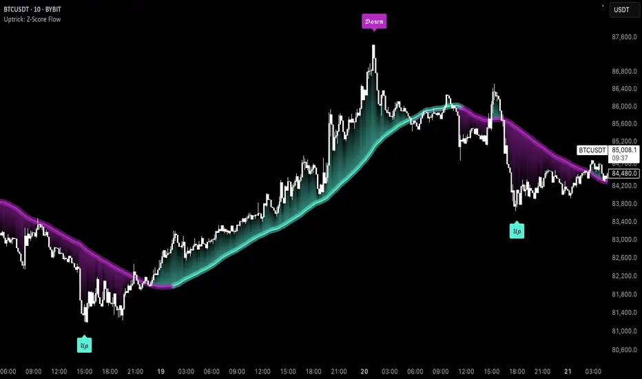
Uptrick: Z-Score FlowOverview
Uptrick: Z-Score Flow is a technical indicator that integrates trend-sensitive momentum analysi s with mean-reversion logic derived from Z-Score calculations. Its primary objective is to identify market conditions where price has either stretched too far from its mean (overbought or oversold) or sits at a statistically “normal” range, and then cross-reference this observation with trend direction and RSI-based momentum signals. The result is a more contextual approach to trade entry and exit, emphasizing precision, clarity, and adaptability across varying market regimes.
Introduction
Financial instruments frequently transition between trending modes, where price extends strongly in one direction, and ranging modes, where price oscillates around a central value. A simple statistical measure like Z-Score can highlight price extremes by comparing the current price against its historical mean and standard deviation. However, such extremes alone can be misleading if the broader market structure is trending forcefully. Uptrick: Z-Score Flow aims to solve this gap by combining Z-Score with an exponential moving average (EMA) trend filter and a smoothed RSI momentum check, thus filtering out signals that contradict the prevailing market environment.
Purpose
The purpose of this script is to help traders pinpoint both mean-reversion opportunities and trend-based pullbacks in a way that is statistically grounded yet still mindful of overarching price action. By pairing Z-Score thresholds with supportive conditions, the script reduces the likelihood of acting on random price spikes or dips and instead focuses on movements that are significant within both historical and current contextual frameworks.
Originality and Uniquness
Layered Signal Verification: Signals require the fulfillment of multiple layers (Z-Score extreme, EMA trend bias, and RSI momentum posture) rather than merely breaching a statistical threshold.
RSI Zone Lockout: Once RSI enters an overbought/oversold zone and triggers a signal, the script locks out subsequent signals until RSI recovers above or below those zones, limiting back-to-back triggers.
Controlled Cooldown: A dedicated cooldown mechanic ensures that the script waits a specified number of bars before issuing a new signal in the opposite direction.
Gradient-Based Visualization: Distinct gradient fills between price and the Z-Mean line enhance readability, showing at a glance whether price is trading above or below its statistical average.
Comprehensive Metrics Panel: An optional on-chart table summarizes the Z-Score’s key metrics, streamlining the process of verifying current statistical extremes, mean levels, and momentum directions.
Why these indicators were merged
Z-Score measurements excel at identifying when price deviates from its mean, but they do not intrinsically reveal whether the market’s trajectory supports a reversion or if price might continue along its trend. The EMA, commonly used for spotting trend directions, offers valuable insight into whether price is predominantly ascending or descending. However, relying solely on a trend filter overlooks the intensity of price moves. RSI then adds a dedicated measure of momentum, helping confirm if the market’s energy aligns with a potential reversal (for example, price is statistically low but RSI suggests looming upward momentum). By uniting these three lenses—Z-Score for statistical context, EMA for trend direction, and RSI for momentum force—the script offers a more comprehensive and adaptable system, aiming to avoid false positives caused by focusing on just one aspect of price behavior.
Calculations
The core calculation begins with a simple moving average (SMA) of price over zLen bars, referred to as the basis. Next, the script computes the standard deviation of price over the same window. Dividing the difference between the current price and the basis by this standard deviation produces the Z-Score, indicating how many standard deviations the price is from its mean. A positive Z-Score reveals price is above its average; a negative reading indicates the opposite.
To detect overall market direction, the script calculates an exponential moving average (emaTrend) over emaTrendLen bars. If price is above this EMA, the script deems the market bullish; if below, it’s considered bearish. For momentum confirmation, the script computes a standard RSI over rsiLen bars, then applies a smoothing EMA over rsiEmaLen bars. This smoothed RSI (rsiEma) is monitored for both its absolute level (oversold or overbought) and its slope (the difference between the current and previous value). Finally, slopeIndex determines how many bars back the script compares the basis to check whether the Z-Mean line is generally rising, falling, or flat, which then informs the coloring scheme on the chart.
Calculations and Rational
Simple Moving Average for Baseline: An SMA is used for the core mean because it places equal weight on each bar in the lookback period. This helps maintain a straightforward interpretation of overbought or oversold conditions in the context of a uniform historical average.
Standard Deviation for Volatility: Standard deviation measures the variability of the data around the mean. By dividing price’s difference from the mean by this value, the Z-Score can highlight whether price is unusually stretched given typical volatility.
Exponential Moving Average for Trend: Unlike an SMA, an EMA places more emphasis on recent data, reacting quicker to new price developments. This quicker response helps the script promptly identify trend shifts, which can be crucial for filtering out signals that go against a strong directional move.
RSI for Momentum Confirmation: RSI is an oscillator that gauges price movement strength by comparing average gains to average losses over a set period. By further smoothing this RSI with another EMA, short-lived oscillations become less influential, making signals more robust.
SlopeIndex for Slope-Based Coloring: To clarify whether the market’s central tendency is rising or falling, the script compares the basis now to its level slopeIndex bars ago. A higher current reading indicates an upward slope; a lower reading, a downward slope; and similar readings, a flat slope. This is visually represented on the chart, providing an immediate sense of the directionality.
Inputs
zLen (Z-Score Period)
Specifies how many bars to include for computing the SMA and standard deviation that form the basis of the Z-Score calculation. Larger values produce smoother but slower signals; smaller values catch quick changes but may generate noise.
emaTrendLen (EMA Trend Filter)
Sets the length of the EMA used to detect the market’s primary direction. This is pivotal for distinguishing whether signals should be considered (price aligning with an uptrend or downtrend) or filtered out.
rsiLen (RSI Length)
Defines the window for the initial RSI calculation. This RSI, when combined with the subsequent smoothing EMA, forms the foundation for momentum-based signal confirmations.
rsiEmaLen (EMA of RSI Period)
Applies an exponential moving average over the RSI readings for additional smoothing. This step helps mitigate rapid RSI fluctuations that might otherwise produce whipsaw signals.
zBuyLevel (Z-Score Buy Threshold)
Determines how negative the Z-Score must be for the script to consider a potential oversold signal. If the Z-Score dives below this threshold (and other criteria are met), a buy signal is generated.
zSellLevel (Z-Score Sell Threshold)
Determines how positive the Z-Score must be for a potential overbought signal. If the Z-Score surpasses this threshold (and other checks are satisfied), a sell signal is generated.
cooldownBars (Cooldown (Bars))
Enforces a bar-based delay between opposite signals. Once a buy signal has fired, the script must wait the specified number of bars before registering a new sell signal, and vice versa.
slopeIndex (Slope Sensitivity (Bars))
Specifies how many bars back the script compares the current basis for slope coloration. A bigger slopeIndex highlights larger directional trends, while a smaller number emphasizes shorter-term shifts.
showMeanLine (Show Z-Score Mean Line)
Enables or disables the plotting of the Z-Mean and its slope-based coloring. Traders who prefer minimal chart clutter may turn this off while still retaining signals.
Features
Statistical Core (Z-Score Detection):
This feature computes the Z-Score by taking the difference between the current price and the basis (SMA) and dividing by the standard deviation. In effect, it translates price fluctuations into a standardized measure that reveals how significant a move is relative to the typical variation seen over the lookback. When the Z-Score crosses predefined thresholds (zBuyLevel for oversold and zSellLevel for overbought), it signals that price could be at an extreme.
How It Works: On each bar, the script updates the SMA and standard deviation. The Z-Score is then refreshed accordingly. Traders can interpret particularly large negative or positive Z-Score values as scenarios where price is abnormally low or high.
EMA Trend Filter:
An EMA over emaTrendLen bars is used to classify the market as bullish if the price is above it and bearish if the price is below it. This classification is applied to the Z-Score signals, accepting them only when they align with the broader price direction.
How It Works: If the script detects a Z-Score below zBuyLevel, it further checks if price is actually in a downtrend (below EMA) before issuing a buy signal. This might seem counterintuitive, but a “downtrend” environment plus an oversold reading often signals a potential bounce or a mean-reversion play. Conversely, for sell signals, the script checks if the market is in an uptrend first. If it is, an overbought reading aligns with potential profit-taking.
RSI Momentum Confirmation with Oversold/Overbought Lockout:
RSI is calculated over rsiLen, then smoothed by an EMA over rsiEmaLen. If this smoothed RSI dips below a certain threshold (for example, 30) and then begins to slope upward, the indicator treats it as a potential sign of recovering momentum. Similarly, if RSI climbs above a certain threshold (for instance, 70) and starts to slope downward, that suggests dwindling momentum. Additionally, once RSI is in these zones, the indicator locks out repetitive signals until RSI fully exits and re-enters those extreme territories.
How It Works: Each bar, the script measures whether RSI has dropped below the oversold threshold (like 30) and has a positive slope. If it does, the buy side is considered “unlocked.” For sell signals, RSI must exceed an overbought threshold (70) and slope downward. The combination of threshold and slope helps confirm that a reversal is genuinely in progress instead of issuing signals while momentum remains weak or stuck in extremes.
Cooldown Mechanism:
The script features a custom bar-based cooldown that prevents issuing new signals in the opposite direction immediately after one is triggered. This helps avoid whipsaw situations where the market quickly flips from oversold to overbought or vice versa.
How It Works: When a buy signal fires, the indicator notes the bar index. If the Z-Score and RSI conditions later suggest a sell, the script compares the current bar index to the last buy signal’s bar index. If the difference is within cooldownBars, the signal is disallowed. This ensures a predefined “quiet period” before switching signals.
Slope-Based Coloring (Z-Mean Line and Shadow):
The script compares the current basis value to its value slopeIndex bars ago. A higher reading now indicates a generally upward slope, while a lower reading indicates a downward slope. The script then shades the Z-Mean line in a corresponding bullish or bearish color, or remains neutral if little change is detected.
How It Works: This slope calculation is refreshingly straightforward: basis – basis . If the result is positive, the line is colored bullish; if negative, it is colored bearish; if approximately zero, it remains neutral. This provides a quick visual cue of the medium-term directional bias.
Gradient Overlays:
With gradient fills, the script highlights where price stands in relation to the Z-Mean. When price is above the basis, a purple-shaded region is painted, visually indicating a “bearish zone” for potential overbought conditions. When price is below, a teal-like overlay is used, suggesting a “bullish zone” for potential oversold conditions.
How It Works: Each bar, the script checks if price is above or below the basis. It then applies a fill between close and basis, using distinct colors to show whether the market is trading above or below its mean. This creates an immediate sense of how extended the market might be.
Buy and Sell Labels (with Alerts):
When a legitimate buy or sell condition passes every check (Z-Score threshold, EMA trend alignment, RSI gating, and cooldown clearance), the script plots a corresponding label directly on the chart. It also fires an alert (if alerts are set up), making it convenient for traders who want timely notifications.
How It Works: If rawBuy or rawSell conditions are met (refined by RSI, EMA trend, and cooldown constraints), the script calls the respective plot function to paint an arrow label on the chart. Alerts are triggered simultaneously, carrying easily recognizable messages.
Metrics Table:
The optional on-chart table (activated by showMetrics) presents real-time Z-Score data, including the current Z-Score, its rolling mean, the maximum and minimum Z-Score values observed over the last zLen bars, a percentile position, and a short-term directional note (rising, falling, or flat).
Current – The present Z-Score reading
Mean – Average Z-Score over the zLen period
Min/Max – Lowest and highest Z-Score values within zLen
Position – Where the current Z-Score sits between the min and max (as a percentile)
Trend – Whether the Z-Score is increasing, decreasing, or flat
Conclusion
Uptrick: Z-Score Flow offers a versatile solution for traders who need a statistically informed perspective on price extremes combined with practical checks for overall trend and momentum. By leveraging a well-defined combination of Z-Score, EMA trend classification, RSI-based momentum gating, slope-based visualization, and a cooldown mechanic, the script reduces the occurrence of false or premature signals. Its gradient fills and optional metrics table contribute further clarity, ensuring that users can quickly assess market posture and make more confident trading decisions in real time.
Disclaimer
This script is intended solely for informational and educational purposes. Trading in any financial market comes with substantial risk, and there is no guarantee of success or the avoidance of loss. Historical performance does not ensure future results. Always conduct thorough research and consider professional guidance prior to making any investment or trading decisions.
[GYTS-CE] Market Regime Detector🧊 Market Regime Detector (Community Edition)
🌸 Part of GoemonYae Trading System (GYTS) 🌸
🌸 --------- INTRODUCTION --------- 🌸
💮 What is the Market Regime Detector?
The Market Regime Detector is an advanced, consensus-based indicator that identifies the current market state to increase the probability of profitable trades. By distinguishing between trending (bullish or bearish) and cyclic (range-bound) market conditions, this detector helps you select appropriate tactics for different environments. Instead of forcing a single strategy across all market conditions, our detector allows you to adapt your approach based on real-time market behaviour.
💮 The Importance of Market Regimes
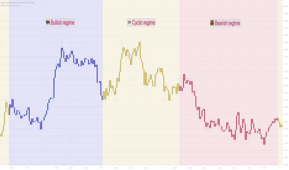
Markets constantly shift between different behavioural states or "regimes":
• Bullish trending markets - characterised by sustained upward price movement
• Bearish trending markets - characterised by sustained downward price movement
• Cyclic markets - characterised by range-bound, oscillating behaviour
Each regime requires fundamentally different trading approaches. Trend-following strategies excel in trending markets but fail in cyclic ones, while mean-reversion strategies shine in cyclic markets but underperform in trending conditions. Detecting these regimes is essential for successful trading, which is why we've developed the Market Regime Detector to accurately identify market states using complementary detection methods.
🌸 --------- KEY FEATURES --------- 🌸
💮 Consensus-Based Detection
Rather than relying on a single method, our detector employs two complementary detection methodologies that analyse different aspects of market behaviour:
• Dominant Cycle Average (DCA) - analyzes price movement relative to its lookback period, a proxy for the dominant cycle
• Volatility Channel - examines price behaviour within adaptive volatility bands
These diverse perspectives are synthesised into a robust consensus that minimises false signals while maintaining responsiveness to genuine regime changes.
💮 Dominant Cycle Framework
The Market Regime Detector uses the concept of dominant cycles to establish a reference framework. You can input the dominant cycle period that best represents the natural rhythm of your market, providing a stable foundation for regime detection across different timeframes.
💮 Intuitive Parameter System
We've distilled complex technical parameters into intuitive controls that traders can easily understand:
• Adaptability - how quickly the detector responds to changing market conditions
• Sensitivity - how readily the detector identifies transitions between regimes
• Consensus requirement - how much agreement is needed among detection methods
This approach makes the detector accessible to traders of all experience levels while preserving the power of the underlying algorithms.
💮 Visual Market Feedback
The detector provides clear visual feedback about the current market regime through:
• Colour-coded chart backgrounds (purple shades for bullish, pink for bearish, yellow for cyclic)
• Colour-coded price bars
• Strength indicators showing the degree of consensus
• Customizable colour schemes to match your preferences or trading system
💮 Integration in the GYTS suite
The Market Regime Detector is compatible with the GYTS Suite , i.e. it passes the regime into the 🎼 Order Orchestrator where you can set how to trade the trending and cyclic regime.
🌸 --------- CONFIGURATION SETTINGS --------- 🌸
💮 Adaptability
Controls how quickly the Market Regime detector adapts to changing market conditions. You can see it as a low-frequency, long-term change parameter:
Very Low: Very slow adaptation, most stable but may miss regime changes
Low: Slower adaptation, more stability but less responsiveness
Normal: Balanced between stability and responsiveness
High: Faster adaptation, more responsive but less stable
Very High: Very fast adaptation, highly responsive but may generate false signals
This setting affects lookback periods and filter parameters across all detection methods.
💮 Sensitivity
Controls how sensitive the detector is to market regime transitions. This acts as a high-frequency, short-term change parameter:
Very Low: Requires substantial evidence to identify a regime change
Low: Less sensitive, reduces false signals but may miss some transitions
Normal: Balanced sensitivity suitable for most markets
High: More sensitive, detects subtle regime changes but may have more noise
Very High: Very sensitive, detects minor fluctuations but may produce frequent changes
This setting affects thresholds for regime detection across all methods.
💮 Dominant Cycle Period
This parameter allows you to specify the market's natural rhythm in bars. This represents a complete market cycle (up and down movement). Finding the right value for your specific market and timeframe might require some experimentation, but it's a crucial parameter that helps the detector accurately identify regime changes. Most of the times the cycle is between 20 and 40 bars.
💮 Consensus Mode
Determines how the signals from both detection methods are combined to produce the final market regime:
• Any Method (OR) : Signals bullish/bearish if either method detects that regime. If methods conflict (one bullish, one bearish), the stronger signal wins. More sensitive, catches more regime changes but may produce more false signals.
• All Methods (AND) : Signals only when both methods agree on the regime. More conservative, reduces false signals but might miss some legitimate regime changes.
• Weighted Decision : Balances both methods with equal weighting. Provides a middle ground between sensitivity and stability.
Each mode also calculates a continuous regime strength value that's used for colour intensity in the 'unconstrained' display mode.
💮 Display Mode
Choose how to display the market regime colours:
• Unconstrained regime: Shows the regime strength as a continuous gradient. This provides more nuanced visualisation where the intensity of the colour indicates the strength of the trend.
• Consensus only: Shows only the final consensus regime with fixed colours based on the detected regime type.
The background and bar colours will change to indicate the current market regime:
• Purple shades: Bullish trending market (darker purple indicates stronger bullish trend)
• Pink shades: Bearish trending market (darker pink indicates stronger bearish trend)
• Yellow: Cyclic (range-bound) market
💮 Custom Colour Options
The Market Regime Detector allows you to customize the colour scheme to match your personal preferences or to coordinate with other indicators:
• Use custom colours: Toggle to enable your own colour choices instead of the default scheme
• Transparency: Adjust the transparency level of all regime colours
• Bullish colours: Define custom colours for strong, medium, weak, and very weak bullish trends
• Bearish colours: Define custom colours for strong, medium, weak, and very weak bearish trends
• Cyclic colour: Define a custom colour for cyclic (range-bound) market conditions
🌸 --------- DETECTION METHODS --------- 🌸
💮 Dominant Cycle Average (DCA)
The Dominant Cycle Average method forms a key part of our detection system:
1. Theoretical Foundation :
The DCA method builds on cycle analysis and the observation that in trending markets, price consistently remains on one side of a moving average calculated using the dominant cycle period. In contrast, during cyclic markets, price oscillates around this average.
2. Calculation Process :
• We calculate a Simple Moving Average (SMA) using the specified lookback period - a proxy for the dominant cycle period
• We then analyse the proportion of time that price spends above or below this SMA over a lookback window. The theory is that the price should cross the SMA each half cycle, assuming that the dominant cycle period is correct and price follows a sinusoid.
• This lookback window is adaptive, scaling with the dominant cycle period (controlled by the Adaptability setting)
• The different values are standardised and normalised to possess more resolving power and to be more robust to noise.
3. Regime Classification :
• When the normalised proportion exceeds a positive threshold (determined by Sensitivity setting), the market is classified as bullish trending
• When it falls below a negative threshold, the market is classified as bearish trending
• When the proportion remains between these thresholds, the market is classified as cyclic
💮 Volatility Channel
The Volatility Channel method complements the DCA method by focusing on price movement relative to adaptive volatility bands:
1. Theoretical Foundation :
This method is based on the observation that trending markets tend to sustain movement outside of normal volatility ranges, while cyclic markets tend to remain contained within these ranges. By creating adaptive bands that adjust to current market volatility, we can detect when price behaviour indicates a trending or cyclic regime.
2. Calculation Process :
• We first calculate a smooth base channel center using a low pass filter, creating a noise-reduced centreline for price
• True Range (TR) is used to measure market volatility, which is then smoothed and scaled by the deviation factor (controlled by Sensitivity)
• Upper and lower bands are created by adding and subtracting this scaled volatility from the centreline
• Price is smoothed using an adaptive A2RMA filter, which has a very flat and stable behaviour, to reduce noise while preserving trend characteristics
• The position of this smoothed price relative to the bands is continuously monitored
3. Regime Classification :
• When smoothed price moves above the upper band, the market is classified as bullish trending
• When smoothed price moves below the lower band, the market is classified as bearish trending
• When price remains between the bands, the market is classified as cyclic
• The magnitude of price's excursion beyond the bands is used to determine trend strength
4. Adaptive Behaviour :
• The smoothing periods and deviation calculations automatically adjust based on the Adaptability setting
• The measured volatility is calculated over a period proportional to the dominant cycle, ensuring the detector works across different timeframes
• Both the center line and the bands adapt dynamically to changing market conditions, making the detector responsive yet stable
This method provides a unique perspective that complements the DCA approach, with the consensus mechanism synthesising insights from both methods.
🌸 --------- USAGE GUIDE --------- 🌸
💮 Starting with Default Settings
The default settings (Normal for Adaptability and Sensitivity, Weighted Decision for Consensus Mode) provide a balanced starting point suitable for most markets and timeframes. Begin by observing how these settings identify regimes in your preferred instruments.
💮 Finding the Optimal Dominant Cycle
The dominant cycle period is a critical parameter. Here are some approaches to finding an appropriate value:
• Start with typical values, usually something around 25 works well
• Visually identify the average distance between significant peaks and troughs
• Experiment with different values and observe which provides the most stable regime identification
• Consider using cycle-finding indicators to help identify the natural rhythm of your market
💮 Adjusting Parameters
• If you notice too many regime changes → Decrease Sensitivity or increase Consensus requirement
• If regime changes seem delayed → Increase Adaptability
• If a trending regime is not detected, the market is automatically assigned to be in a cyclic state
• If you want to see more nuanced regime transitions → Try the "unconstrained" display mode (note that this will not affect the output to other indicators)
💮 Trading Applications
Regime-Specific Strategies:
• Bullish Trending Regime - Use trend-following strategies, trail stops wider, focus on breakouts, consider holding positions longer, and emphasize buying dips
• Bearish Trending Regime - Consider shorts, tighter stops, focus on breakdown points, sell rallies, implement downside protection, and reduce position sizes
• Cyclic Regime - Apply mean-reversion strategies, trade range boundaries, apply oscillators, target definable support/resistance levels, and use profit-taking at extremes
Strategy Switching:
Create a set of rules for each market regime and switch between them based on the detector's signal. This approach can significantly improve performance compared to applying a single strategy across all market conditions.
GYTS Suite Integration:
• In the GYTS 🎼 Order Orchestrator, select the '🔗 STREAM-int 🧊 Market Regime' as the market regime source
• Note that the consensus output (i.e. not the "unconstrained" display) will be used in this stream
• Create different strategies for trending (bullish/bearish) and cyclic regimes. The GYTS 🎼 Order Orchestrator is specifically made for this.
• The output stream is actually very simple, and can possibly be used in indicators and strategies as well. It outputs 1 for bullish, -1 for bearish and 0 for cyclic regime.
🌸 --------- FINAL NOTES --------- 🌸
💮 Development Philosophy
The Market Regime Detector has been developed with several key principles in mind:
1. Robustness - The detection methods have been rigorously tested across diverse markets and timeframes to ensure reliable performance.
2. Adaptability - The detector automatically adjusts to changing market conditions, requiring minimal manual intervention.
3. Complementarity - Each detection method provides a unique perspective, with the collective consensus being more reliable than any individual method.
4. Intuitiveness - Complex technical parameters have been abstracted into easily understood controls.
💮 Ongoing Refinement
The Market Regime Detector is under continuous development. We regularly:
• Fine-tune parameters based on expanded market data
• Research and integrate new detection methodologies
• Optimise computational efficiency for real-time analysis
Your feedback and suggestions are very important in this ongoing refinement process!
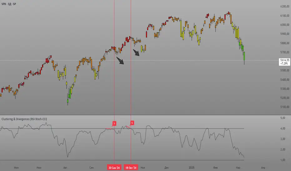
Clustering & Divergences (RSI-Stoch-CCI) [Sam SDF-Solutions]The Clustering & Divergences (RSI-Stoch-CCI) indicator is a comprehensive technical analysis tool that consolidates three popular oscillators—Relative Strength Index (RSI), Stochastic, and Commodity Channel Index (CCI)—into one unified metric called the Score. This Score offers traders an aggregated view of market conditions, allowing them to quickly identify whether the market is oversold, balanced, or overbought.
Functionality:
Oscillator Clustering: The indicator calculates the values of RSI, Stochastic, and CCI using user-defined periods. These oscillator values are then normalized using one of three available methods: MinMax, Z-Score, or Z-Bins.
Score Calculation: Each normalized oscillator value is multiplied by its respective weight (which the user can adjust), and the weighted values are summed to generate an overall Score. This Score serves as a single, interpretable metric representing the combined oscillator behavior.
Market Clustering: The indicator performs clustering on the Score over a configurable window. By dividing the Score range into a set number of clusters (also configurable), the tool visually represents the market’s state. Each cluster is assigned a unique color so that traders can quickly see if the market is trending toward oversold, balanced, or overbought conditions.
Divergence Detection: The script automatically identifies both Regular and Hidden divergences between the price action and the Score. By using pivot detection on both price and Score data, the indicator marks potential reversal signals on the chart with labels and connecting lines. This helps in pinpointing moments when the price and the underlying oscillator dynamics diverge.
Customization Options: Users have full control over the indicator’s behavior. They can adjust:
The periods for each oscillator (RSI, Stochastic, CCI).
The weights applied to each oscillator in the Score calculation.
The normalization method and its manual boundaries.
The number of clusters and whether to invert the cluster order.
Parameters for divergence detection (such as pivot sensitivity and the minimum/maximum bar distance between pivots).
Visual Enhancements:
Depending on the user’s preference, either the Score or the Cluster Index (derived from the clustering process) is plotted on the chart. Additionally, the script changes the color of the price bars based on the identified cluster, providing an at-a-glance visual cue of the current market regime.
Logic & Methodology:
Input Parameters: The script starts by accepting user inputs for clustering settings, oscillator periods, weights, divergence detection, and manual boundary definitions for normalization.
Oscillator Calculation & Normalization: It computes RSI, Stochastic, and CCI values from the price data. These values are then normalized using either the MinMax method (scaling between a lower and upper band) or the Z-Score method (standardizing based on mean and standard deviation), or using Z-Bins for an alternative scaling approach.
Score Computation: Each normalized oscillator is multiplied by its corresponding weight. The sum of these products results in the overall Score that represents the combined oscillator behavior.
Clustering Algorithm: The Score is evaluated over a moving window to determine its minimum and maximum values. Using these values, the script calculates a cluster index that divides the Score into a predefined number of clusters. An option to invert the cluster calculation is provided to adjust the interpretation of the clustering.
Divergence Analysis: The indicator employs pivot detection (using left and right bar parameters) on both the price and the Score. It then compares recent pivot values to detect regular and hidden divergences. When a divergence is found, the script plots labels and optional connecting lines to highlight these key moments on the chart.
Plotting: Finally, based on the user’s selection, the indicator plots either the Score or the Cluster Index. It also overlays manual boundary lines (for the chosen normalization method) and adjusts the bar colors according to the cluster to provide clear visual feedback on market conditions.
_________
By integrating multiple oscillator signals into one cohesive tool, the Clustering & Divergences (RSI-Stoch-CCI) indicator helps traders minimize subjective analysis. Its dynamic clustering and automated divergence detection provide a streamlined method for assessing market conditions and potentially enhancing the accuracy of trading decisions.
For further details on using this indicator, please refer to the guide available at:
2:30 [LuciTech]this is a technical analysis tool designed to highlight key price levels and patterns during a specific trading window, based on UK time (Europe/London). It overlays visual elements on the chart, including a 12 PM reference line, Buy Side Liquidity (BSL) and Sell Side Liquidity (SSL) levels, a highlighted 2:30 PM candle, and Engulfing Fair Value Gaps (FVGs). This indicator is intended for traders who focus on intraday price action and liquidity zones.
Features
The 12 PM Line displays a vertical line at 12:00 PM (UK time) to mark the start of the session. It’s customizable, allowing you to enable or disable it and adjust its color.
BSL/SSL Lines track the highest high (BSL) and lowest low (SSL) from 12:00 PM to 2:00 PM (UK time). These lines extend horizontally until 3:30 PM, after which they remain static at their last recorded levels. You can customize them by enabling or disabling visibility, adjusting colors, choosing a line style (solid, dashed, or dotted), and setting the width.
The 2:30 PM Candle highlights the candle at 2:30 PM (UK time) with a distinct color. It’s customizable, with options to enable or disable it and change its color.
Engulfing FVG (Fair Value Gap) identifies bullish and bearish engulfing patterns with a gap from the prior candle’s range. It draws a shaded box over the FVG area, and you can customize it by enabling or disabling it and adjusting the box color.
How It Works
The indicator operates within a session starting at 12:00 PM (UK time). BSL/SSL levels update between 12:00 PM and 2:00 PM, with lines extending until 3:30 PM. After 3:30 PM, these lines freeze.
BSL/SSL lines show the highest price (BSL) and lowest price (SSL) reached during the 12:00 PM to 2:00 PM window. After 3:30 PM, they remain static, marking the final range boundaries.
The 2:30 PM candle emphasizes a key timestamp, often of interest to intraday traders.
Engulfing FVGs detect significant price gaps created by engulfing candles, which may indicate potential reversal or continuation zones.
Settings
12 PM Line Settings let you toggle visibility and set the line color.
BSL/SSL Line Settings allow you to toggle visibility, set BSL and SSL colors, choose a line style (Solid, Dashed, Dotted), and adjust width (1-4).
2:30 Candle Settings let you toggle visibility and set the candle color.
Engulfing FVG Settings allow you to toggle visibility and set the box color.
Interpretation
The 12 PM Line serves as a reference for the session start.
BSL/SSL Lines may act as potential support or resistance zones or highlight liquidity areas. After 3:30 PM, they remain static, showing the session’s final range.
The 2:30 PM Candle can be monitored for price action signals, such as reversals or breakouts.
Engulfing FVGs shaded areas may indicate imbalances in supply and demand, useful for identifying trade opportunities or stop-loss placement.
Notes
The timezone is set to Europe/London (UK time). Ensure your chart’s timezone aligns for accurate results.
This indicator is best used on intraday timeframes, such as 1-minute or 5-minute charts.
It provides visual aids for analysis and does not generate buy or sell signals on its own.

CBC Strategy with Trend Confirmation & Separate Stop LossCBC Flip Strategy with Trend Confirmation and ATR-Based Targets
This strategy is based on the CBC Flip concept taught by MapleStax and inspired by the original CBC Flip indicator by AsiaRoo. It focuses on identifying potential reversals or trend continuation points using a combination of candlestick patterns (CBC Flips), trend filters, and a time-based entry window. This approach helps traders avoid false signals and increase trade accuracy.
What is a CBC Flip?
The CBC Flip is a candlestick-based pattern that identifies moments when the market is likely to change direction or strengthen its trend. It checks for a shift in price behavior between consecutive candles, signaling a bullish (upward) or bearish (downward) move.
However, not all flips are created equal! This strategy differentiates between Strong Flips and All Flips, allowing traders to choose between a more conservative or aggressive approach.
Strong Flips vs. All Flips
Strong Flips
A Strong Flip is a high-probability setup that occurs only after liquidity is swept from the previous candle’s high or low.
What is a liquidity sweep? This happens when the price briefly moves beyond the high or low of the previous candle, triggering stop-losses and trapping traders in the wrong direction. These sweeps often create fuel for the next move, making them powerful reversal signals.
Examples:
Long Setup: The price dips below the previous candle’s low (sweeping liquidity) and then closes higher, signaling a potential bullish move.
Short Setup: The price moves above the previous candle’s high and then closes lower, signaling a potential bearish move.
Why Use Strong Flips?
They provide fewer signals, but the accuracy is generally higher.
Ideal for trending markets where liquidity sweeps often mark key turning points.
All Flips
All Flips are less selective, offering both Strong Flips and additional signals without requiring a liquidity sweep.
This approach gives traders more frequent opportunities but comes with a higher risk of false signals, especially in sideways markets.
Examples:
Long Setup: A CBC flip occurs without sweeping the previous low, but the trend direction is confirmed (slow EMA is still above VWAP).
Short Setup: A CBC flip occurs without sweeping the previous high, but the trend is still bearish (slow EMA below VWAP).
Why Use All Flips?
Provides more frequent entries for active or aggressive traders.
Works well in trending markets but requires caution during consolidation periods.
How This Strategy Works
The strategy combines CBC Flips with multiple filters to ensure better trade quality:
Trend Confirmation: The slow EMA (20-period) must be positioned relative to the VWAP to confirm the overall trend direction.
Long Trades: Slow EMA must be above VWAP (upward trend).
Short Trades: Slow EMA must be below VWAP (downward trend).
Time-Based Filter: Traders can specify trading hours to limit entries to a particular time window, helping avoid low-volume or high-volatility periods.
Profit Target and Stop-Loss:
Profit Target: Defined as a multiple of the 14-period ATR (Average True Range). For example, if the ATR is 10 points and the profit target multiplier is set to 1.5, the strategy aims for a 15-point profit.
Stop-Loss: Uses a dynamic, candle-based stop-loss:
Long Trades: The trade closes if the market closes below the low of two candles ago.
Short Trades: The trade closes if the market closes above the high of two candles ago.
This approach adapts to recent price behavior and protects against unexpected reversals.
Customizable Settings
Strong Flips vs. All Flips: Choose between a more selective or aggressive entry style.
Profit Target Multiplier: Adjust the ATR multiplier to control the distance for profit targets.
Entry Time Range: Define specific trading hours for the strategy.
Indicators and Visuals
Fast EMA (10-Period) – Black Line
Slow EMA (20-Period) – Red Line
VWAP (Volume-Weighted Average Price) – Orange Line
Visual Labels:
▵ (Triangle Up) – Marks long entries (buy signals).
▿ (Triangle Down) – Marks short entries (sell signals).
Credits
CBC Flip Concept: Inspired by MapleStax, who teaches this concept.
Original Indicator: Developed by AsiaRoo, this strategy builds on the CBC Flip framework with additional features for improved trade management.
Risks and Disclaimer
This strategy is for educational purposes only and does not constitute financial advice.
Trading involves significant risk and may result in the loss of capital. Past performance does not guarantee future results. Use this strategy in a simulated environment before applying it to live trading.

JJ Highlight Time Ranges with First 5 Minutes and LabelsTo effectively use this Pine Script as a day trader , here’s how the various elements can help you manage trades, track time sessions, and monitor price movements:
Key Components for a Day Trader:
1. First 5-Minute Highlight:
- Purpose: Day traders often rely on the first 5 minutes of the trading session to gauge market sentiment, watch for opening price gaps, or plan entries. This script draws a horizontal line at the high or low of the first 5 minutes, which can act as a key level for the rest of the day.
- How to Use: If the price breaks above or below the first 5-minute line, it can signal momentum. You might enter a long position if the price breaks above the first 5-minute high or a short if it breaks below the first 5-minute low.
2. Session Time Highlights:
- Morning Session (9:15–10:30 AM): The market often shows its strongest price action during the first hour of trading. This session is highlighted in yellow. You can use this highlight to focus on the most volatile period, as this is when large institutional moves tend to occur.
- Afternoon Session (12:30–2:55 PM): The blue highlight helps you track the mid-afternoon session, where liquidity may decrease, and price action can sometimes be choppier. Day traders should be more cautious during this period.
- How to Use: By highlighting these key times, you can:
- Focus on key breakouts during the morning session.
- Be more conservative in your trades during the afternoon, as market volatility may drop.
3. Dynamic Labels:
- Top/Bottom Positioning: The script places labels dynamically based on the selected position (Top or Bottom). This allows you to quickly glance at the session's start and identify where you are in terms of time.
- How to Use: Use these labels to remind yourself when major time segments (morning or afternoon) begin. You can adjust your trading strategy depending on the session, e.g., being more aggressive in the morning and more cautious in the afternoon.
Trading Strategy Suggestions:
1. Momentum Trades:
- After the first 5 minutes, use the high/low of that period to set up breakout trades.
- Long Entry: If the price breaks the high of the first 5 minutes (especially if there's a strong trend).
- Short Entry: If the price breaks the low of the first 5 minutes, signaling a potential downtrend.
2. Session-Based Strategy:
- Morning Session (9:15–10:30 AM):
- Look for strong breakout patterns such as support/resistance levels, moving average crossovers, or candlestick patterns (like engulfing candles or pin bars).
- This is a high liquidity period, making it ideal for executing quick trades.
- Afternoon Session (12:30–2:55 PM):
- The market tends to consolidate or show less volatility. Scalping and mean-reversion strategies work better here.
- Avoid chasing big moves unless you see a clear breakout in either direction.
3. Support and Resistance:
- The first 5-minute high/low often acts as a key support or resistance level for the rest of the day. If the price holds above or below this level, it’s an indication of trend continuation.
4. Breakout Confirmation:
- Look for breakouts from the highlighted session time ranges (e.g., 9:15 AM–10:30 AM or 12:30 PM–2:55 PM).
- If a breakout happens during a key time window, combine that with other technical indicators like volume spikes , RSI , or MACD for confirmation.
---
Example Day Trader Usage:
1. First 5 Minutes Strategy: After the market opens at 9:15 AM, watch the price action for the first 5 minutes. The high and low of these 5 minutes are critical levels. If the price breaks above the high of the first 5 minutes, it might indicate a strong bullish trend for the day. Conversely, breaking below the low may suggest bearish movement.
2. Morning Session: After the first 5 minutes, focus on the **9:15 AM–10:30 AM** window. During this time, look for breakout setups at key support/resistance levels, especially when paired with high volume or momentum indicators. This is when many institutions make large trades, so price action tends to be more volatile and predictable.
3. Afternoon Session: From 12:30 PM–2:55 PM, the market might experience lower volatility, making it ideal for scalping or range-bound strategies. You could look for reversals or fading strategies if the market becomes too quiet.
Conclusion:
As a day trader, you can use this script to:
- Track and react to key price levels during the first 5 minutes.
- Focus on high volatility in the morning session (9:15–10:30 AM) and **be cautious** during the afternoon.
- Use session-based timing to adjust your strategies based on the time of day.
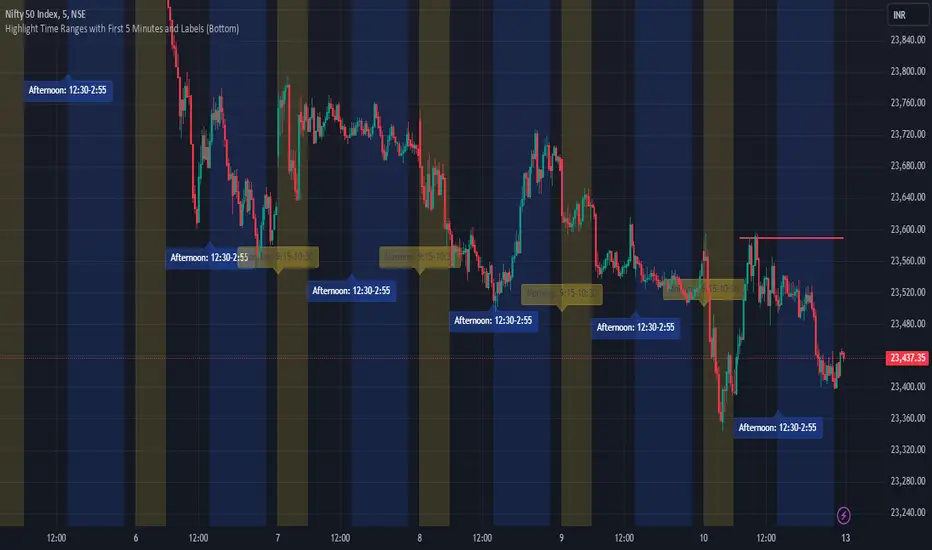
PIP Algorithm
# **Script Overview (For Non-Coders)**
1. **Purpose**
- The script tries to capture the essential “shape” of price movement by selecting a limited number of “key points” (anchors) from the latest bars.
- After selecting these anchors, it draws straight lines between them, effectively simplifying the price chart into a smaller set of points without losing major swings.
2. **How It Works, Step by Step**
1. We look back a certain number of bars (e.g., 50).
2. We start by drawing a straight line from the **oldest** bar in that range to the **newest** bar—just two points.
3. Next, we find the bar whose price is *farthest away* from that straight line. That becomes a new anchor point.
4. We “snap” (pin) the line to go exactly through that new anchor. Then we re-draw (re-interpolate) the entire line from the first anchor to the last, in segments.
5. We repeat the process (adding more anchors) until we reach the desired number of points. Each time, we choose the biggest gap between our line and the actual price, then re-draw the entire shape.
6. Finally, we connect these anchors on the chart with red lines, visually simplifying the price curve.
3. **Why It’s Useful**
- It highlights the most *important* bends or swings in the price over the chosen window.
- Instead of plotting every single bar, it condenses the information down to the “key turning points.”
4. **Key Takeaway**
- You’ll see a small number of red line segments connecting the **most significant** points in the price data.
- This is especially helpful if you want a simplified view of recent price action without minor fluctuations.
## **Detailed Logic Explanation**
# **Script Breakdown (For Coders)**
//@version=5
indicator(title="PIP Algorithm", overlay=true)
// 1. Inputs
length = input.int(50, title="Lookback Length")
num_points = input.int(5, title="Number of PIP Points (≥ 3)")
// 2. Helper Functions
// ---------------------------------------------------------------------
// reInterpSubrange(...):
// Given two “anchor” indices in `linesArr`, linearly interpolate
// the array values in between so that the subrange forms a straight line
// from linesArr to linesArr .
reInterpSubrange(linesArr, segmentLeft, segmentRight) =>
float leftVal = array.get(linesArr, segmentLeft)
float rightVal = array.get(linesArr, segmentRight)
int segmentLen = segmentRight - segmentLeft
if segmentLen > 1
for i = segmentLeft + 1 to segmentRight - 1
float ratio = (i - segmentLeft) / segmentLen
float interpVal = leftVal + (rightVal - leftVal) * ratio
array.set(linesArr, i, interpVal)
// reInterpolateAllSegments(...):
// For the entire “linesArr,” re-interpolate each subrange between
// consecutive breakpoints in `lineBreaksArr`.
// This ensures the line is globally correct after each new anchor insertion.
reInterpolateAllSegments(linesArr, lineBreaksArr) =>
array.sort(lineBreaksArr, order.asc)
for i = 0 to array.size(lineBreaksArr) - 2
int leftEdge = array.get(lineBreaksArr, i)
int rightEdge = array.get(lineBreaksArr, i + 1)
reInterpSubrange(linesArr, leftEdge, rightEdge)
// getMaxDistanceIndex(...):
// Return the index (bar) that is farthest from the current “linesArr.”
// We skip any indices already in `lineBreaksArr`.
getMaxDistanceIndex(linesArr, closeArr, lineBreaksArr) =>
float maxDist = -1.0
int maxIdx = -1
int sizeData = array.size(linesArr)
for i = 1 to sizeData - 2
bool isBreak = false
for b = 0 to array.size(lineBreaksArr) - 1
if i == array.get(lineBreaksArr, b)
isBreak := true
break
if not isBreak
float dist = math.abs(array.get(linesArr, i) - array.get(closeArr, i))
if dist > maxDist
maxDist := dist
maxIdx := i
maxIdx
// snapAndReinterpolate(...):
// "Snap" a chosen index to its actual close price, then re-interpolate the entire line again.
snapAndReinterpolate(linesArr, closeArr, lineBreaksArr, idxToSnap) =>
if idxToSnap >= 0
float snapVal = array.get(closeArr, idxToSnap)
array.set(linesArr, idxToSnap, snapVal)
reInterpolateAllSegments(linesArr, lineBreaksArr)
// 3. Global Arrays and Flags
// ---------------------------------------------------------------------
// We store final data globally, then use them outside the barstate.islast scope to draw lines.
var float finalCloseData = array.new_float()
var float finalLines = array.new_float()
var int finalLineBreaks = array.new_int()
var bool didCompute = false
var line pipLines = array.new_line()
// 4. Main Logic (Runs Once at the End of the Current Bar)
// ---------------------------------------------------------------------
if barstate.islast
// A) Prepare closeData in forward order (index 0 = oldest bar, index length-1 = newest)
float closeData = array.new_float()
for i = 0 to length - 1
array.push(closeData, close )
// B) Initialize linesArr with a simple linear interpolation from the first to the last point
float linesArr = array.new_float()
float firstClose = array.get(closeData, 0)
float lastClose = array.get(closeData, length - 1)
for i = 0 to length - 1
float ratio = (length > 1) ? (i / float(length - 1)) : 0.0
float val = firstClose + (lastClose - firstClose) * ratio
array.push(linesArr, val)
// C) Initialize lineBreaks with two anchors: 0 (oldest) and length-1 (newest)
int lineBreaks = array.new_int()
array.push(lineBreaks, 0)
array.push(lineBreaks, length - 1)
// D) Iteratively insert new breakpoints, always re-interpolating globally
int iterationsNeeded = math.max(num_points - 2, 0)
for _iteration = 1 to iterationsNeeded
// 1) Re-interpolate entire shape, so it's globally up to date
reInterpolateAllSegments(linesArr, lineBreaks)
// 2) Find the bar with the largest vertical distance to this line
int maxDistIdx = getMaxDistanceIndex(linesArr, closeData, lineBreaks)
if maxDistIdx == -1
break
// 3) Insert that bar index into lineBreaks and snap it
array.push(lineBreaks, maxDistIdx)
array.sort(lineBreaks, order.asc)
snapAndReinterpolate(linesArr, closeData, lineBreaks, maxDistIdx)
// E) Save results into global arrays for line drawing outside barstate.islast
array.clear(finalCloseData)
array.clear(finalLines)
array.clear(finalLineBreaks)
for i = 0 to array.size(closeData) - 1
array.push(finalCloseData, array.get(closeData, i))
array.push(finalLines, array.get(linesArr, i))
for b = 0 to array.size(lineBreaks) - 1
array.push(finalLineBreaks, array.get(lineBreaks, b))
didCompute := true
// 5. Drawing the Lines in Global Scope
// ---------------------------------------------------------------------
// We cannot create lines inside barstate.islast, so we do it outside.
array.clear(pipLines)
if didCompute
// Connect each pair of anchors with red lines
if array.size(finalLineBreaks) > 1
for i = 0 to array.size(finalLineBreaks) - 2
int idxLeft = array.get(finalLineBreaks, i)
int idxRight = array.get(finalLineBreaks, i + 1)
float x1 = bar_index - (length - 1) + idxLeft
float x2 = bar_index - (length - 1) + idxRight
float y1 = array.get(finalCloseData, idxLeft)
float y2 = array.get(finalCloseData, idxRight)
line ln = line.new(x1, y1, x2, y2, extend=extend.none)
line.set_color(ln, color.red)
line.set_width(ln, 2)
array.push(pipLines, ln)
1. **Data Collection**
- We collect the **most recent** `length` bars in `closeData`. Index 0 is the oldest bar in that window, index `length-1` is the newest bar.
2. **Initial Straight Line**
- We create an array called `linesArr` that starts as a simple linear interpolation from `closeData ` (the oldest bar’s close) to `closeData ` (the newest bar’s close).
3. **Line Breaks**
- We store “anchor points” in `lineBreaks`, initially ` `. These are the start and end of our segment.
4. **Global Re-Interpolation**
- Each time we want to add a new anchor, we **re-draw** (linear interpolation) for *every* subrange ` [lineBreaks , lineBreaks ]`, ensuring we have a globally consistent line.
- This avoids the “local subrange only” approach, which can cause clustering near existing anchors.
5. **Finding the Largest Distance**
- After re-drawing, we compute the vertical distance for each bar `i` that isn’t already a line break. The bar with the biggest distance from the line is chosen as the next anchor (`maxDistIdx`).
6. **Snapping and Re-Interpolate**
- We “snap” that bar’s line value to the actual close, i.e. `linesArr = closeData `. Then we globally re-draw all segments again.
7. **Repeat**
- We repeat these insertions until we have the desired number of points (`num_points`).
8. **Drawing**
- Finally, we connect each consecutive pair of anchor points (`lineBreaks`) with a `line.new(...)` call, coloring them red.
- We offset the line’s `x` coordinate so that the anchor at index 0 lines up with `bar_index - (length - 1)`, and the anchor at index `length-1` lines up with `bar_index` (the current bar).
**Result**:
You get a simplified representation of the price with a small set of line segments capturing the largest “jumps” or swings. By re-drawing the entire line after each insertion, the anchors tend to distribute more *evenly* across the data, mitigating the issue where anchors bunch up near each other.
Enjoy experimenting with different `length` and `num_points` to see how the simplified lines change!
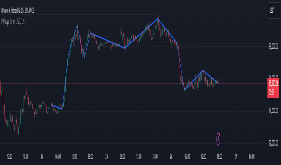
300-Candle Weighted Average Zones w/50 EMA SignalsThis indicator is designed to deliver a more nuanced view of price dynamics by combining a custom, weighted price average with a volatility-based zone and a trend filter (in this case, a 50-period exponential moving average). The core concept revolves around capturing the overall price level over a relatively large lookback window (300 candles) but with an intentional bias toward recent market activity (the most recent 20 candles), thereby offering a balance between long-term context and short-term responsiveness. By smoothing this weighted average and establishing a “zone” of standard deviation bands around it, the indicator provides a refined visualization of both average price and its recent volatility envelope. Traders can then look for confluence with a standard trend filter, such as the 50 EMA, to identify meaningful crossover signals that may represent trend shifts or opportunities for entry and exit.
What the Indicator Does:
Weighted Price Average:
Instead of using a simple or exponential moving average, this indicator calculates a custom weighted average price over the past 300 candles. Most historical candles receive a base weight of 1.0, but the most recent 20 candles are assigned a higher weight (for example, a weight of 2.0). This weighting scheme ensures that the calculation is not simply a static lookback average; it actively emphasizes current market conditions. The effect is to generate an average line that is more sensitive to the most recent price swings while still maintaining the historical context of the previous 280 candles.
Smoothing of the Weighted Average:
Once the raw weighted average is computed, an exponential smoothing function (EMA) is applied to reduce noise and produce a cleaner, more stable average line. This smoothing helps traders avoid reacting prematurely to minor price fluctuations. By stabilizing the average line, traders can more confidently identify actual shifts in market direction.
Volatility Zone via Standard Deviation Bands:
To contextualize how far price can deviate from this weighted average, the indicator uses standard deviation. Standard deviation is a statistical measure of volatility—how spread out the price values are around the mean. By adding and subtracting one standard deviation from the smoothed weighted average, the indicator plots an upper band and a lower band, creating a zone or channel. The area between these bands is filled, often with a semi-transparent color, highlighting a volatility corridor within which price and the EMA might oscillate.
This zone is invaluable in visualizing “normal” price behavior. When the 50 EMA line and the weighted average line are both within this volatility zone, it indicates that the market’s short- to mid-term trend and its average pricing are aligned well within typical volatility bounds.
Incorporation of a 50-Period EMA:
The inclusion of a commonly used trend filter, the 50 EMA, adds another layer of context to the analysis. The 50 EMA, being a widely recognized moving average length, is often considered a baseline for intermediate trend bias. It reacts faster than a long-term average (like a 200 EMA) but is still stable enough to filter out the market “chop” seen in very short-term averages.
By overlaying the 50 EMA on this custom weighted average and the surrounding volatility zone, the trader gains a dual-dimensional perspective:
Trend Direction: If the 50 EMA is generally above the weighted average, the short-term trend is gaining bullish momentum; if it’s below, the short-term trend has a bearish tilt.
Volatility Normalization: The bands, constructed from standard deviations, provide a sense of whether the price and the 50 EMA are operating within a statistically “normal” range. If the EMA crosses the weighted average within this zone, it signals a potential trend initiation or meaningful shift, as opposed to a random price spike outside normal volatility boundaries.
Why a Trader Would Want to Use This Indicator:
Contextualized Price Level:
Standard MAs may not fully incorporate the most recent price dynamics in a large lookback window. By weighting the most recent candles more heavily, this indicator ensures that the trader is always anchored to what the market is currently doing, not just what it did 100 or 200 candles ago.
Reduced Whipsaw with Smoothing:
The smoothed weighted average line reduces noise, helping traders filter out inconsequential price movements. This makes it easier to spot genuine changes in trend or sentiment.
Visual Volatility Gauge:
The standard deviation bands create a visual representation of “normal” price movement. Traders can quickly assess if a breakout or breakdown is statistically significant or just another oscillation within the expected volatility range.
Clear Trade Signals with Confirmation:
By integrating the 50 EMA and designing signals that trigger only when the 50 EMA crosses above or below the weighted average while inside the zone, the indicator provides a refined entry/exit criterion. This avoids chasing breakouts that occur in abnormal volatility conditions and focuses on those crossovers likely to have staying power.
How to Use It in an Example Strategy:
Imagine you are a swing trader looking to identify medium-term trend changes. You apply this indicator to a chart of a popular currency pair or a leading tech stock. Over the past few days, the 50 EMA has been meandering around the weighted average line, both confined within the standard deviation zone.
Bullish Example:
Suddenly, the 50 EMA crosses decisively above the weighted average line while both are still hovering within the volatility zone. This might be your cue: you interpret this crossover as the 50 EMA acknowledging the recent upward shift in price dynamics that the weighted average has highlighted. Since it occurred inside the normal volatility range, it’s less likely to be a head-fake. You place a long position, setting an initial stop just below the lower band to protect against volatility.
If the price continues to rise and the EMA stays above the average, you have confirmation to hold the trade. As the price moves higher, the weighted average may follow, reinforcing your bullish stance.
Bearish Example:
On the flip side, if the 50 EMA crosses below the weighted average line within the zone, it suggests a subtle but meaningful change in trend direction to the downside. You might short the asset, placing your protective stop just above the upper band, expecting that the statistically “normal” level of volatility will contain the price action. If the price does break above those bands later, it’s a sign your trade may not work out as planned.
Other Indicators for Confluence:
To strengthen the reliability of the signals generated by this weighted average zone approach, traders may want to combine it with other technical studies:
Volume Indicators (e.g., Volume Profile, OBV):
Confirm that the trend crossover inside the volatility zone is supported by volume. For instance, an uptrend crossover combined with increasing On-Balance Volume (OBV) or volume spikes on up candles signals stronger buying pressure behind the price action.
Momentum Oscillators (e.g., RSI, Stochastics):
Before taking a crossover signal, check if the RSI is above 50 and rising for bullish entries, or if the Stochastics have turned down from overbought levels for bearish entries. Momentum confirmation can help ensure that the trend change is not just an isolated random event.
Market Structure Tools (e.g., Pivot Points, Swing High/Low Analysis):
Identify if the crossover event coincides with a break of a previous pivot high or low. A bullish crossover inside the zone aligned with a break above a recent swing high adds further strength to your conviction. Conversely, a bearish crossover confirmed by a breakdown below a previous swing low can make a short trade setup more compelling.
Volume-Weighted Average Price (VWAP):
Comparing where the weighted average zone lies relative to VWAP can provide institutional insight. If the bullish crossover happens while the price is also holding above VWAP, it can mean that the average participant in the market is in profit and that the trend is likely supported by strong hands.
This indicator serves as a tool to balance long-term perspective, short-term adaptability, and volatility normalization. It can be a valuable addition to a trader’s toolkit, offering enhanced clarity and precision in detecting meaningful shifts in trend, especially when combined with other technical indicators and robust risk management principles.

Blue Sniper V.1Overview
This Pine Script indicator is designed to generate Buy and Sell signals based on proximity to the 50 EMA, stochastic oscillator levels, retracement conditions, and EMA slopes. It is tailored for trending market conditions, making it ideal for identifying high-probability entry points during strong bullish or bearish trends.
Key Features:
Filters out signals in non-trending conditions.
Focuses on retracements near the 50 EMA for precise entries.
Supports alert notifications for Buy and Sell signals.
Includes a cooldown mechanism to prevent signal spamming.
Allows time-based filtering to restrict signals to a specific trading window.
How It Works
Trending Market Conditions
The indicator is most effective when the market exhibits a clear trend. It uses two exponential moving averages (50 EMA and 200 EMA) to determine the overall market trend:
Bullish Trend: 50 EMA is above the 200 EMA, and both EMAs have upward slopes.
Bearish Trend: 50 EMA is below the 200 EMA, and both EMAs have downward slopes.
Buy and Sell Conditions
Buy Signal:
The market is in a bullish trend.
Stochastic oscillator is in the oversold zone.
Price retraces upwards, breaking away from the recent low by more than 1.5 ATR.
Price is near the 50 EMA (within the defined proximity percentage).
Sell Signal:
The market is in a bearish trend.
Stochastic oscillator is in the overbought zone.
Price retraces downwards, breaking away from the recent high by more than 1.5 ATR.
Price is near the 50 EMA.
Outputs
Signals:
Buy Signal: Green "BUY" label below the price bar.
Sell Signal: Red "SELL" label above the price bar.
Alerts:
Alerts are triggered for Buy and Sell signals if conditions are met within the specified time window (if enabled).
EMA Visualization:
50 EMA (blue line).
200 EMA (red line).
Limitations
Not Suitable for Non-Trending Markets: This script is designed for trending conditions. Sideways or choppy markets may produce false signals.
Proximity Tolerance: Adjust the proximityPercent to prevent signals from triggering too frequently during minor oscillations around the 50 EMA.
No Guarantee of Accuracy: As with any technical indicator, it should be used in conjunction with other tools and analysis.
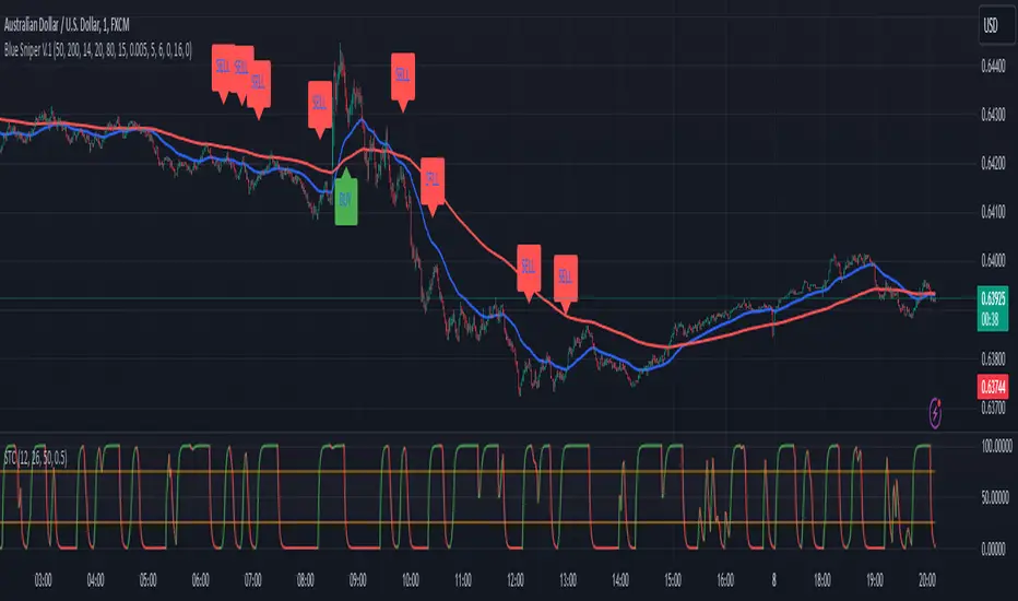
Ensemble Alerts█ OVERVIEW
This indicator creates highly customizable alert conditions and messages by combining several technical conditions into groups , which users can specify directly from the "Settings/Inputs" tab. It offers a flexible framework for building and testing complex alert conditions without requiring code modifications for each adjustment.
█ CONCEPTS
Ensemble analysis
Ensemble analysis is a form of data analysis that combines several "weaker" models to produce a potentially more robust model. In a trading context, one of the most prevalent forms of ensemble analysis is the aggregation (grouping) of several indicators to derive market insights and reinforce trading decisions. With this analysis, traders typically inspect multiple indicators, signaling trade actions when specific conditions or groups of conditions align.
Simplifying ensemble creation
Combining indicators into one or more ensembles can be challenging, especially for users without programming knowledge. It usually involves writing custom scripts to aggregate the indicators and trigger trading alerts based on the confluence of specific conditions. Making such scripts customizable via inputs poses an additional challenge, as it often involves complicated input menus and conditional logic.
This indicator addresses these challenges by providing a simple, flexible input menu where users can easily define alert criteria by listing groups of conditions from various technical indicators in simple text boxes . With this script, you can create complex alert conditions intuitively from the "Settings/Inputs" tab without ever writing or modifying a single line of code. This framework makes advanced alert setups more accessible to non-coders. Additionally, it can help Pine programmers save time and effort when testing various condition combinations.
█ FEATURES
Configurable alert direction
The "Direction" dropdown at the top of the "Settings/Inputs" tab specifies the allowed direction for the alert conditions. There are four possible options:
• Up only : The indicator only evaluates upward conditions.
• Down only : The indicator only evaluates downward conditions.
• Up and down (default): The indicator evaluates upward and downward conditions, creating alert triggers for both.
• Alternating : The indicator prevents alert triggers for consecutive conditions in the same direction. An upward condition must be the first occurrence after a downward condition to trigger an alert, and vice versa for downward conditions.
Flexible condition groups
This script features six text inputs where users can define distinct condition groups (ensembles) for their alerts. An alert trigger occurs if all the conditions in at least one group occur.
Each input accepts a comma-separated list of numbers with optional spaces (e.g., "1, 4, 8"). Each listed number, from 1 to 35, corresponds to a specific individual condition. Below are the conditions that the numbers represent:
1 — RSI above/below threshold
2 — RSI below/above threshold
3 — Stoch above/below threshold
4 — Stoch below/above threshold
5 — Stoch K over/under D
6 — Stoch K under/over D
7 — AO above/below threshold
8 — AO below/above threshold
9 — AO rising/falling
10 — AO falling/rising
11 — Supertrend up/down
12 — Supertrend down/up
13 — Close above/below MA
14 — Close below/above MA
15 — Close above/below open
16 — Close below/above open
17 — Close increase/decrease
18 — Close decrease/increase
19 — Close near Donchian top/bottom (Close > (Mid + HH) / 2)
20 — Close near Donchian bottom/top (Close < (Mid + LL) / 2)
21 — New Donchian high/low
22 — New Donchian low/high
23 — Rising volume
24 — Falling volume
25 — Volume above average (Volume > SMA(Volume, 20))
26 — Volume below average (Volume < SMA(Volume, 20))
27 — High body to range ratio (Abs(Close - Open) / (High - Low) > 0.5)
28 — Low body to range ratio (Abs(Close - Open) / (High - Low) < 0.5)
29 — High relative volatility (ATR(7) > ATR(40))
30 — Low relative volatility (ATR(7) < ATR(40))
31 — External condition 1
32 — External condition 2
33 — External condition 3
34 — External condition 4
35 — External condition 5
These constituent conditions fall into three distinct categories:
• Directional pairs : The numbers 1-22 correspond to pairs of opposing upward and downward conditions. For example, if one of the inputs includes "1" in the comma-separated list, that group uses the "RSI above/below threshold" condition pair. In this case, the RSI must be above a high threshold for the group to trigger an upward alert, and the RSI must be below a defined low threshold to trigger a downward alert.
• Non-directional filters : The numbers 23-30 correspond to conditions that do not represent directional information. These conditions act as filters for both upward and downward alerts. Traders often use non-directional conditions to refine trending or mean reversion signals. For instance, if one of the input lists includes "30", that group uses the "Low relative volatility" condition. The group can trigger an upward or downward alert only if the 7-period Average True Range (ATR) is below the 40-period ATR.
• External conditions : The numbers 31-35 correspond to external conditions based on the plots from other indicators on the chart. To set these conditions, use the source inputs in the "External conditions" section near the bottom of the "Settings/Inputs" tab. The external value can represent an upward, downward, or non-directional condition based on the following logic:
▫ Any value above 0 represents an upward condition.
▫ Any value below 0 represents a downward condition.
▫ If the checkbox next to the source input is selected, the condition becomes non-directional . Any group that uses the condition can trigger upward or downward alerts only if the source value is not 0.
To learn more about using plotted values from other indicators, see this article in our Help Center and the Source input section of our Pine Script™ User Manual.
Group markers
Each comma-separated list represents a distinct group , where all the listed conditions must occur to trigger an alert. This script assigns preset markers (names) to each condition group to make the active ensembles easily identifiable in the generated alert messages and labels. The markers assigned to each group use the format "M", where "M" is short for "Marker" and "x" is the group number. The titles of the inputs at the top of the "Settings/Inputs" tab show these markers for convenience.
For upward conditions, the labels and alert messages show group markers with upward triangles (e.g., "M1▲"). For downward conditions, they show markers with downward triangles (e.g., "M1▼").
NOTE: By default, this script populates the "M1" field with a pre-configured list for a mean reversion group ("2,18,24,28"). The other fields are empty. If any "M*" input does not contain a value, the indicator ignores it in the alert calculations.
Custom alert messages
By default, the indicator's alert message text contains the activated markers and their direction as a comma-separated list. Users can override this message for upward or downward alerts with the two text fields at the bottom of the "Settings/Inputs" tab. When the fields are not empty , the alerts use that text instead of the default marker list.
NOTE: This script generates alert triggers, not the alerts themselves. To set up an alert based on this script's conditions, open the "Create Alert" dialog box, then select the "Ensemble Alerts" and "Any alert() function call" options in the "Condition" tabs. See the Alerts FAQ in our Pine Script™ User Manual for more information.
Condition visualization
This script offers organized visualizations of its conditions, allowing users to inspect the behaviors of each condition alongside the specified groups. The key visual features include:
1) Conditional plots
• The indicator plots the history of each individual condition, excluding the external conditions, as circles at different levels. Opposite conditions appear at positive and negative levels with the same absolute value. The plots for each condition show values only on the bars where they occur.
• Each condition's plot is color-coded based on its type. Aqua and orange plots represent opposing directional conditions, and purple plots represent non-directional conditions. The titles of the plots also contain the condition numbers to which they apply.
• The plots in the separate pane can be turned on or off with the "Show plots in pane" checkbox near the top of the "Settings/Inputs" tab. This input only toggles the color-coded circles, which reduces the graphical load. If you deactivate these visuals, you can still inspect each condition from the script's status line and the Data Window.
• As a bonus, the indicator includes "Up alert" and "Down alert" plots in the Data Window, representing the combined upward and downward ensemble alert conditions. These plots are also usable in additional indicator-on-indicator calculations.
2) Dynamic labels
• The indicator draws a label on the main chart pane displaying the activated group markers (e.g., "M1▲") each time an alert condition occurs.
• The labels for upward alerts appear below chart bars. The labels for downward alerts appear above the bars.
NOTE: This indicator can display up to 500 labels because that is the maximum allowed for a single Pine script.
3) Background highlighting
• The indicator can highlight the main chart's background on bars where upward or downward condition groups activate. Use the "Highlight background" inputs in the "Settings/Inputs" tab to enable these highlights and customize their colors.
• Unlike the dynamic labels, these background highlights are available for all chart bars, irrespective of the number of condition occurrences.
█ NOTES
• This script uses Pine Script™ v6, the latest version of TradingView's programming language. See the Release notes and Migration guide to learn what's new in v6 and how to convert your scripts to this version.
• This script imports our new Alerts library, which features functions that provide high-level simplicity for working with complex compound conditions and alerts. We used the library's `compoundAlertMessage()` function in this indicator. It evaluates items from "bool" arrays in groups specified by an array of strings containing comma-separated index lists , returning a tuple of "string" values containing the marker of each activated group.
• The script imports the latest version of the ta library to calculate several technical indicators not included in the built-in `ta.*` namespace, including Double Exponential Moving Average (DEMA), Triple Exponential Moving Average (TEMA), Fractal Adaptive Moving Average (FRAMA), Tilson T3, Awesome Oscillator (AO), Full Stochastic (%K and %D), SuperTrend, and Donchian Channels.
• The script uses the `force_overlay` parameter in the label.new() and bgcolor() calls to display the drawings and background colors in the main chart pane.
• The plots and hlines use the available `display.*` constants to determine whether the visuals appear in the separate pane.
Look first. Then leap.

Reversal Signals [AlgoAlpha]📈🔄 Reversal Signals – Master Market Reversals with Precision! 🚀✨
Elevate your trading strategy with the Reversal Signals indicator by AlgoAlpha. This advanced tool is designed to pinpoint potential bullish and bearish reversals by analyzing price action and, optionally, volume confirmations. It seamlessly combines reversal detection with trend analysis, giving you a comprehensive view of market dynamics to make informed trading decisions.
Key Features
🔎 Price Action Reversal Detection : Identifies potential reversal points by comparing current price movements against historical candle patterns within a customizable lookback period.
📊 Volume Confirmation : Optionally integrates volume analysis to confirm the strength of reversal signals, enhancing their reliability.
📈 Stepped Moving Average Trend Indicator : Employs a stepped moving average that adjusts at set intervals to reflect underlying market trends.
⚙️ Customizable Settings : Tailor the indicator to your trading style with adjustable parameters for lookback periods, confirmation windows, moving average types, and more.
🎨 Visual Signals and Trend Coloring : Clear on-chart labels for reversal signals and color-coded trend areas to quickly identify bullish and bearish conditions.
🔔 Alerts for Key Market Events : Set up custom alerts for reversal signals and trend shifts to stay ahead of market movements.
Quick Guide to Using the Reversal Signals Indicator :
🛠 Add the Indicator : Add the indicator to your favorites by pressing the star icon. Customize settings like Candle Lookback, Confirm Within, and Use Volume Confirmation to fit your trading style.
📊 Market Analysis : Observe the "𝓡" labels on the chart indicating bullish and bearish reversal signals. Look for labels below the bars for bullish signals and above the bars for bearish signals. Use the color-filled areas between the stepped moving average and the center line to assess market trends.
🔔 Alerts : Enable notifications for reversal signals and trend shifts to stay informed about market movements without constantly monitoring the chart.
How It Works
The Reversal Signals indicator operates by conducting a thorough analysis of price action over a user-defined lookback period. For a bullish reversal, the indicator checks if the current closing price is lower than the lows of the preceding candles within the lookback window, suggesting a potential oversold condition. If this criterion is met, it marks the candle as a potential reversal point and waits for confirmation within a specified number of subsequent candles. Confirmation occurs when the price rises above the high of the identified candle, signaling a bullish reversal. An optional volume confirmation can be enabled to ensure that the reversal is supported by higher-than-average trading volume, adding an extra layer of validation to the signal. The process is mirrored for bearish reversals, where the indicator looks for the closing price exceeding previous highs and awaits confirmation of a downward move.
Complementing the reversal signals, the indicator features a stepped moving average that serves as a dynamic trend indicator. This moving average updates at intervals defined by the MA Step Period and shifts direction based on price crossings. If the price remains above the stepped MA, it indicates a bullish trend, coloring the area between the MA and the center line in green. Conversely, if the price falls below the stepped MA, a bearish trend is signaled, and the area is shaded red. This visual representation helps traders quickly assess the prevailing market trend and align their trading decisions accordingly.
Experience a new level of market insight with the Reversal Signals indicator. Add it to your TradingView chart today and enhance your ability to detect and act on key ma

Enhanced Market Analyzer with Adaptive Cognitive LearningThe "Enhanced Market Analyzer with Advanced Features and Adaptive Cognitive Learning" is an advanced, multi-dimensional trading indicator that leverages sophisticated algorithms to analyze market trends and generate predictive trading signals. This indicator is designed to merge traditional technical analysis with modern machine learning techniques, incorporating features such as adaptive learning, Monte Carlo simulations, and probabilistic modeling. It is ideal for traders who seek deeper market insights, adaptive strategies, and reliable buy/sell signals.
Key Features:
Adaptive Cognitive Learning:
Utilizes Monte Carlo simulations, reinforcement learning, and memory feedback to adapt to changing market conditions.
Adjusts the weighting and learning rate of signals dynamically to optimize predictions based on historical and real-time data.
Hybrid Technical Indicators:
Custom RSI Calculation: An RSI that adapts its length based on recursive learning and error adjustments, making it responsive to varying market conditions.
VIDYA with CMO Smoothing: An advanced moving average that incorporates Chander Momentum Oscillator for adaptive smoothing.
Hamming Windowed VWMA: A volume-weighted moving average that applies a Hamming window for smoother calculations.
FRAMA: A fractal adaptive moving average that responds dynamically to price movements.
Advanced Statistical Analysis:
Skewness and Kurtosis: Provides insights into the distribution and potential risk of market trends.
Z-Score Calculations: Identifies extreme market conditions and adjusts trading thresholds dynamically.
Probabilistic Monte Carlo Simulation:
Runs thousands of simulations to assess potential price movements based on momentum, volatility, and volume factors.
Integrates the results into a probabilistic signal that informs trading decisions.
Feature Extraction:
Calculates a variety of market metrics, including price change, momentum, volatility, volume change, and ATR.
Normalizes and adapts these features for use in machine learning algorithms, enhancing signal accuracy.
Ensemble Learning:
Combines signals from different technical indicators, such as RSI, MACD, Bollinger Bands, Stochastic Oscillator, and statistical features.
Weights each signal based on cumulative performance and learning feedback to create a robust ensemble signal.
Recursive Memory and Feedback:
Stores and averages past RSI calculations in a memory array to provide historical context and improve future predictions.
Adaptive memory factor adjusts the influence of past data based on current market conditions.
Multi-Factor Dynamic Length Calculation:
Determines the length of moving averages based on volume, volatility, momentum, and rate of change (ROC).
Adapts to various market conditions, ensuring that the indicator is responsive to both high and low volatility environments.
Adaptive Learning Rate:
The learning rate can be adjusted based on market volatility, allowing the system to adapt its speed of learning and sensitivity to changes.
Enhances the system's ability to react to different market regimes.
Monte Carlo Simulation Engine:
Simulates thousands of random outcomes to model potential future price movements.
Weights and aggregates these simulations to produce a final probabilistic signal, providing a comprehensive risk assessment.
RSI with Dynamic Adjustments:
The initial RSI length is adjusted recursively based on calculated errors between true RSI and predicted RSI.
The adaptive RSI calculation ensures that the indicator remains effective across various market phases.
Hybrid Moving Averages:
Short-Term and Long-Term Averages: Combines FRAMA, VIDYA, and Hamming VWMA with specific weights for a unique hybrid moving average.
Weighted Gradient: Applies a color gradient to indicate trend strength and direction, improving visual clarity.
Signal Generation:
Generates buy and sell signals based on the ensemble model and multi-factor analysis.
Uses percentile-based thresholds to determine overbought and oversold conditions, factoring in historical data for context.
Optional settings to enable adaptation to volume and volatility, ensuring the indicator remains effective under different market conditions.
Monte Carlo and Learning Parameters:
Users can customize the number of Monte Carlo simulations, learning rate, memory factor, and reward decay for tailored performance.
Applications:
Scalping and Day Trading:
The fast response of the adaptive RSI and ensemble learning model makes this indicator suitable for short-term trading strategies.
Swing Trading:
The combination of long-term moving averages and probabilistic models provides reliable signals for medium-term trends.
Volatility Analysis:
The ATR, Bollinger Bands, and adaptive moving averages offer insights into market volatility, helping traders adjust their strategies accordingly.
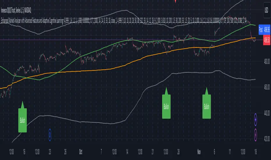
Standard Deviation OscillatorStandard Deviation Oscillator (STDEV OSC) v1.1
Description
The Standard Deviation Oscillator transforms traditional volatility measurements into a dynamic oscillator that fluctuates between 0 and 100. This advanced technical analysis tool helps traders identify periods of extreme volatility and potential market turning points.
Features
Normalized volatility readings (0-100 scale)
Dynamic color changes based on volatility levels
Customizable overbought/oversold thresholds
Built-in alert conditions
Adaptive calculation using rolling windows
Clean, professional visualization
Indicator Parameters
Length: 20; Calculation period for standard deviation
Source: close; Price source for calculations
Overbought Level: 70; Upper threshold for high volatility
Oversold Level: 30; Lower threshold for low volatility
Visual Components
- Main Oscillator Line: Changes color based on current level
- Red: Above overbought level
- Green: Below oversold level
- Blue: Normal range
- Reference Lines:
- Overbought level (default: 70)
- Oversold level (default: 30)
- Middle line (50)
Alert Conditions
1. Volatility High Alert
- Triggers when oscillator crosses above the overbought level
- Useful for identifying potential market tops or breakout scenarios
2. Volatility Low Alert
- Triggers when oscillator crosses below the oversold level
- Helps identify potential market bottoms or consolidation periods
Risk Adjustment Tool
- Scale position sizes inversely to oscillator readings
- Reduce exposure during extremely high volatility periods
- Increase position sizes during normal volatility conditions
Best Practices
1. Timeframe Selection
- Best suited for 1H, 4H, and Daily charts
- Adjust length parameter based on timeframe
2. Confirmation
- Use in conjunction with trend indicators
- Confirm signals with price action patterns
- Consider overall market context
3. Parameter Optimization
- Backtest different length settings
- Adjust overbought/oversold levels based on asset
- Consider market conditions when setting alerts
Technical Notes
- Built in PineScript v5
- Optimized for TradingView platform
- Uses rolling window calculations for better adaptability
- Compatible with all trading instruments
- Minimal performance impact on charts
Version History
- v1.1: Added dynamic coloring, customizable levels, and alert conditions
- v1.0: Initial release with basic oscillator functionality
Disclaimer
This technical indicator is provided for educational and informational purposes only. Past performance is not indicative of future results. Always conduct thorough testing and use proper risk management techniques.
---
Tags: #TechnicalAnalysis #Volatility #Trading #Oscillator #TradingView #PineScript
