IU Probability CalculatorHow This Script Works:
1. This script calculate the probability of price reaching a user-defined price level within one candle with the help Normal Distribution Probability Table.
2. Normal Distribution Probability Table is use for calculating probability of events, it's very powerful for calculation of probability and this script is fully based on that table.
3. It takes the Average True Range value or Standard Deviation value of past user-defined length bar.
4. After that it take this formula z = ( price_level - close ) / (ATR or Standard Deviation) and return the value for z, for the bearish side it take z = (close - price level) / (ATR or Standard Deviation ) formula.
5. Once we have the z it look into Normal Distribution Probability Table and match the value.
6. Now the value of z is multiple buy 100 in order to make it look in percentage term.
7. After that this script subtract the final value with 100 because probability always comes under 100%
8. finally we plot the probability at the bottom of the chart the red line indicates "The probability of price not reaching that price level", While the green line indicates "Probability of price Reaching that level " .
9. This script will work fine for both of the directions
How This Is Useful For The User:
1. With this script user can know the probability of price reaching the certain level within one candle for both Directions .
2. This is useful while creating options hedging strategies
3. This can be helpful for deciding stop loss level.
4. It's useful for scalpers for managing their traders and it can be use by binary option traders.
Cerca negli script per "想象图:箱线图+折线组合,横轴为国家,纵轴为响应指数(0-100),箱线显示均值±标准差,叠加红色虚线标注各国确诊高峰时间点"

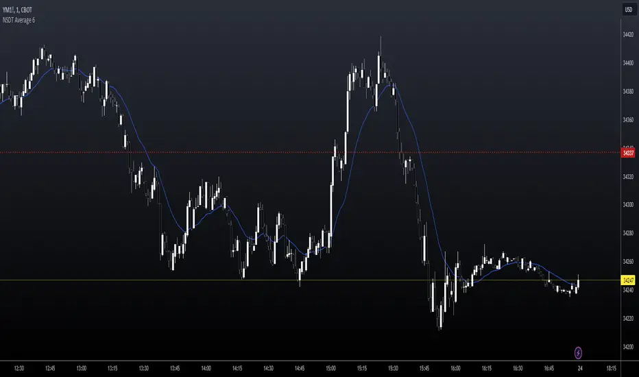
NSDT Average 6This is a pretty simple concept that we were asked to put together. It uses 6 Moving Averages, and takes the average of each one, then averages them all together.
If you don't want to use 6, and only 3 for example, then just enter the same length in two of the input fields as pairs.
Example:
For 6, you could use 10, 20, 30, 40, 50, 60
For 3, you could use 10, 10, 50, 50, 100, 100
It doesn't ploy 6 MA's, it only plots one - the result of the average of an average of an average, etc..
Publishing open source so other can modify as needed.
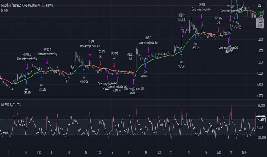
Trend_Trader_WMA (Momentum)<---> Caution! This is first test version of indicator. I am ready to get more ideas+feedback to develop it more. <--->
The "Momentum_Trader_WMA" indicator is a versatile technical analysis tool designed to help traders identify potential trend changes and momentum shifts in the market. It combines multiple indicators and moving averages to provide a comprehensive view of price action and momentum.
Key Features:
Weighted Moving Averages (WMAs): The indicator calculates two different WMAs with user-defined lengths, providing a smoothed representation of price data.
Average True Range (ATR) Bands: ATR is used to calculate dynamic bands around the WMA Average. These bands can help traders gauge market volatility and potential breakout points. The color of the ATR bands can be seen as an early signal of trends or the continuation of current trends.
Commodity Channel Index (CCI): CCI is a momentum oscillator that measures the relative strength of price changes. The indicator calculates CCI values based on a user-defined period.
Exponential Moving Average (EMA) of CCI: An EMA of CCI is plotted to help identify trends and momentum shifts.
Color-Coded Bands: The ATR bands change colors based on CCI conditions, providing visual cues for potential trading opportunities. When ATR bands transition from narrow (indicating low volatility) to wide (indicating increased volatility), it can be seen as an early signal of a potential trend change or the continuation of the current trend.
Buy and Sell Signals: The indicator generates buy and sell signals based on crossovers of WMAs and CCI thresholds, making it easier for traders to identify entry and exit points.
Customizable Moving Averages: Traders can enable or disable different moving averages (e.g., SMA, EMA, WMA, RMA, VWMA, HMA) with various periods and colors to adapt the indicator to their trading preferences.
CCI Dot Alerts: Dots are displayed at the bottom of the chart based on CCI values, helping traders spot extreme CCI conditions.
How to Use:
Trend Identification: The WMAs and ATR bands can help identify the current trend direction and its strength. When the WMAs are in an uptrend (green) and the ATR bands widen, it may indicate a strong bullish trend. Conversely, when the WMAs are in a downtrend (red) and the ATR bands narrow, it may suggest a weakening bearish trend.
Momentum Confirmation: The CCI and its EMA provide insights into market momentum. Look for CCI crossovers above 100 for potential bullish momentum and below -100 for potential bearish momentum.
Buy and Sell Signals: Pay attention to the buy and sell signals generated by the indicator. Buy when the WMAs cross over and CCI crosses above 100. Sell when the WMAs cross under and CCI crosses below -100.
ATR Bands as Early Signals: The color changes in the ATR bands can be seen as early signals of trends or the continuation of current trends. Wide ATR bands may indicate increased volatility and potential trend changes, while narrow ATR bands suggest reduced volatility and potential trend continuation.
Moving Averages: Customize the indicator by enabling or disabling specific moving averages according to your preferred trading strategy.
CCI Dots: Use the CCI dots to identify extreme CCI conditions, which may indicate overbought or oversold market conditions.
PS:
Recommended to use Indicator with price action conecpts(eg. support and resistance) as they play important role in any market.
Buy and sell signals are not really accurate. I would personally look for trend shift in WMA middle line and confirmation from CCI dots at bottom. For example. If middle line turns green and within recent 3-4 candles (or next 3-4 candles) dots tunrns green also, that means momentum has been rised in the direction of bulls.
pls, take s/r concepts first when working. I am thinking to add more precise buy sell signal method to make it easier to trade.
Good luck with your trades :)

ATR Based EMA Price Targets [SS]As requested...
This is a spinoff of my EMA 9/21 cross indicator with price targets.
A few of you asked for a simple EMA crossover version and that is what this is.
I have, of course, added a bit of extra functionality to it, assuming you would want to transition from another EMA indicator to this one, I tried to leave it somewhat customizable so you can get the same type of functionality as any other EMA based indicator just with the added advantage of having an ATR based assessment added on. So lets get into the details:
What it does:
Same as my EMA 9/21, simply performs a basic ATR range analysis on a ticker, calculating the average move it does on a bullish or bearish cross.
How to use it:
So there are quite a few functions of this indicator. I am going to break them down one by one, from most basic to the more complex.
Plot functions:
EMA is Customizable: The EMA is customizable. If you want the 200, 100, 50, 31, 9, whatever you want, you just have to add the desired EMA timeframe in the settings menu.
Standard Deviation Bands are an option: If you like to have standard deviation bands added to your EMA's, you can select to show the standard deviation band. It will plot the standard deviation for the desired EMA timeframe (so if it is the EMA 200, it will plot the Standard Deviation on the EMA 200).
Plotting Crossovers: You can have the indicator plot green arrows for bullish crosses and red arrows for bearish crosses. I have smoothed out this function slightly by only having it signal a crossover when it breaks and holds. I pulled this over to the alert condition functions as well, so you are not constantly being alerted when it is bouncing over and below an EMA. Only once it chooses a direction, holds and moves up or down, will it alert to a true crossover.
Plotting labels: The indicator will default to plotting the price target labels and the EMA label. You can toggle these on and off in the EMA settings menu.
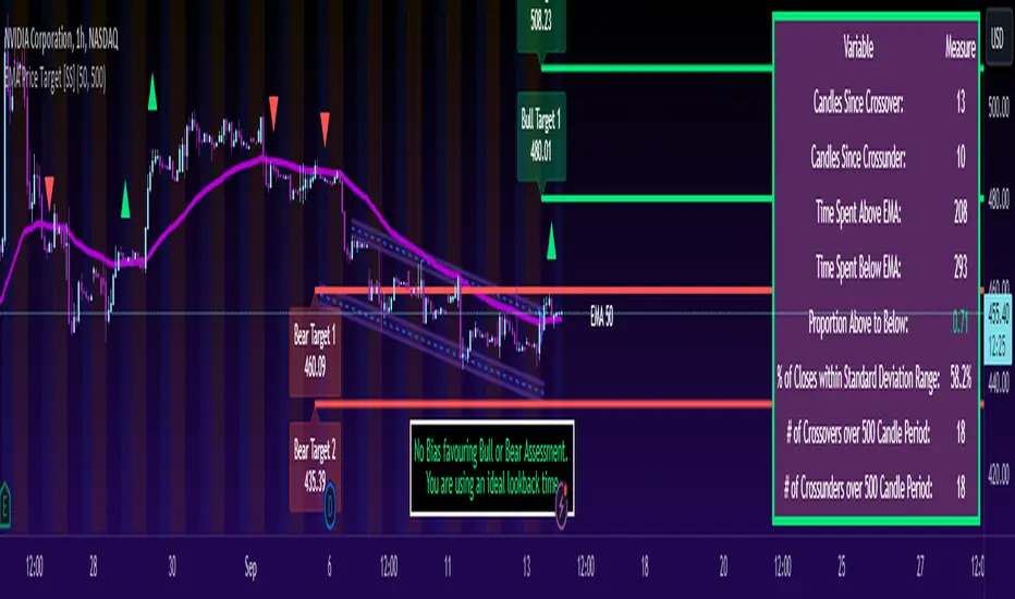
Trend Assessment Settings:
In addition to plotting the EMA itself and signaling the ATR ranges, the EMA will provide you will demographic information about the trend and price action behaviour around the EMA. You can see an example in the image below:
This will provide you with a breakdown of the statistics on the EMA over the designated lookback period, such as the number of crosses, the time above and below the EMA and the amount the EMA has remained within its standard deviation bands.
Where this is important is the proportion assessment. And what the proportion assessment is doing is its measuring the amount of time the ticker is spending either above or below the EMA.
Ideally, you should have relatively equal and uniform durations above and below. This would be a proportion of between 0.5 and 1.5 Above to Below. Now, you don't have to remember this because you can ask the indicator to do the assessment for you. It will be displayed at the bottom of your chart in a table that you can toggle on and off:
Example of a Uniform Assessment:
Example of a biased assessment:
Keep in mind, if you are using those very laggy EMAs (like the 50, 200, 100 etc.) on the daily timeframe, you aren't going to get uniformity in the data. This is because, stocks are technically already biased to the upside over time. Thus, when you are looking at the big picture, the bull bias thesis of the stock market is in play.
But for the smaller and moderate timeframes, owning to the randomness of price action, you can generally get uniformity in data representation by simply adjusting your lookback period.
To adjust your lookback period, you simply need to change the timeframe for the ATR lookback length. I suggest no less than 500 and probably no more than 1,500 candles, and work within this range. But you can use what the indicator indicates is appropriate.
Of course, all of these charts can be turned off and you are left with a clean looking EMA indicator:
And an example with the standard deviation bands toggled on:
And that, my friends, is the indicator.
Hopefully this is what you wanted, let me know if you have any suggestions.
Enjoy and safe trades!
[blackcat] L1 Reverse Choppiness IndexThe Choppiness Index is a technical indicator that is used to measure market volatility and trendiness. It is designed to help traders identify when the market is trending and when it is choppy, meaning that it is moving sideways with no clear direction. The Choppiness Index was first introduced by Australian commodity trader E.W. Dreiss in the late 1990s, and it has since become a popular tool among traders.
Today, I created a reverse version of choppiness index indicator, which uses upward direction as indicating strong trend rather than a traditional downward direction. Also, it max values are exceeding 100 compared to a traditional one. I use red color to indicate a strong trend, while yellow as sideways. Fuchsia zone are also incorporated as an indicator of sideways. One thing that you need to know: different time frames may need optimize parameters of this indicator. Finally, I'd be happy to explain more about this piece of code.
The code begins by defining two input variables: `len` and `atrLen`. `len` sets the length of the lookback period for the highest high and lowest low, while `atrLen` sets the length of the lookback period for the ATR calculation.
The `atr()` function is then used to calculate the ATR, which is a measure of volatility based on the range of price movement over a certain period of time. The `highest()` and `lowest()` functions are used to calculate the highest high and lowest low over the lookback period specified by `len`.
The `range`, `up`, and `down` variables are then calculated based on the highest high, lowest low, and closing price. The `sum()` function is used to calculate the sum of ranges over the lookback period.
Finally, the Choppiness Index is calculated using the ATR and the sum of ranges over the lookback period. The `log10()` function is used to take the logarithm of the sum divided by the lookback period, and the result is multiplied by 100 to get a percentage. The Choppiness Index is then plotted on the chart using the `plot()` function.
This code can be used directly in TradingView to plot the Choppiness Index on a chart. It can also be incorporated into custom trading strategies to help traders make more informed decisions based on market volatility and trendiness.
I hope this explanation helps! Let me know if you have any further questions.

CCI RSI Trading SignalThe "CCI RSI Trading Signal" indicator combines the Commodity Channel Index (CCI) and Relative Strength Index (RSI) to provide buy and sell signals for trading. The CCI identifies potential trend reversals, while the RSI helps confirm overbought and oversold conditions.
How It Works:
The indicator generates a buy signal when the CCI crosses above -100 (indicating a potential bullish reversal) and the RSI is below the specified oversold level. On the other hand, a sell signal is produced when the CCI crosses below 100 (indicating a potential bearish reversal) and the RSI is above the specified overbought level.
Customization:
Traders can adjust the RSI and CCI periods, RSI oversold and overbought levels, as well as take profit, stop loss, and lot size settings to suit their trading preferences.
Usage:
The "CCI RSI Trading Signal" indicator can be used on various timeframes and markets to aid in decision-making, providing potential entry and exit points based on the combined analysis of CCI and RSI.
Rectified BB% for option tradingThis indicator shows the bollinger bands against the price all expressed in percentage of the mean BB value. With one sight you can see the amplitude of BB and the variation of the price, evaluate a reenter of the price in the BB.
The relative price is visualized as a candle with open/high/low/close value exspressed as percentage deviation from the BB mean
The indicator include a modified RSI, remapped from 0/100 to -100/100.
You can choose the BB parameters (length, standard deviation multiplier) and the RSI parameter (length, overbougth threshold, ovrsold threshold)
You can exclude/include the candles and the RSI line.
The indicator can be used to sell options when the volatility is high (the bollinger band is wide) and the price is reentering inside the bands.
If the price is forming a supply or demand area it can be a good opportunity to sell a bull put or a bear call
The RSI can be used as confirm of the supply/demand formation
If the bollinger band is narrow and the RSI is overbought/oversold it indicate a better opportunity to buy options
the indicator is designed to work with daily timeframe and default parameters.

imlibLibrary "imlib"
Description
The library allows you to display images in your scripts utilising the objects. You can change the image size and screen aspect ratio (the ratio of width to height which you can change if the image is too wide / tall). The library has "example()" function which you can use to see how it works. It also has a handy "logo()" function which you can use to quickly display an image by passing the "Image data string", table position, image size and aspect ratio. And of course you can use it in your own custom way by taking the "logo()" function as an example and modifying the code to your needs.
Since tables in Pinescript are limited to 100 by 100 cells, the limit for image's size is also 100x100 px. All the necessary data to display an image is passed as a string variable, and since Pinescript has a limit of 4096 characters for variables of type, that string can have a maximum length of 4096 characters, which is enough to display a 64x64px image (but can be enough to display a 100x100 image, depending on the image itself).
Below you can find the definitions of functions for this library.
_decompress(data)
: Decompresses string with data image
Parameters:
data (string)
Returns: : Array of with decompressed data
load(data)
: Splits the string with image data into components and builds an object
Parameters:
data (string)
Returns: : An object
show(imgdata, table_id, image_size, screen_ratio)
: Displays an image in a table
Parameters:
imgdata (ImgData)
table_id (table)
image_size (float)
screen_ratio (string)
Returns: : nothing
example()
: Use it as an example of how this library works and how to use it in your own scripts
Returns: : nothing
logo(imgdata, position, image_size, screen_ratio)
: Displays logo using image data string
Parameters:
imgdata (string)
position (string)
image_size (float)
screen_ratio (string)
Returns: : nothing
ImgData
Fields:
w (series__integer)
h (series__integer)
s (series__string)
pal (series__string)
data (array__string)

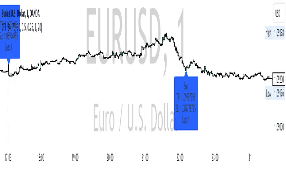
CCI+EMA Strategy with Percentage or ATR TP/SL [Alifer]This is a momentum strategy based on the Commodity Channel Index (CCI), with the aim of entering long trades in oversold conditions and short trades in overbought conditions.
Optionally, you can enable an Exponential Moving Average (EMA) to only allow trading in the direction of the larger trend. Please note that the strategy will not plot the EMA. If you want, for visual confirmation, you can add to the chart an Exponential Moving Average as a second indicator, with the same settings used in the strategy’s built-in EMA.
The strategy also allows you to set internal Stop Loss and Take Profit levels, with the option to choose between Percentage-based TP/SL or ATR-based TP/SL.
The strategy can be adapted to multiple assets and timeframes:
Pick an asset and a timeframe
Zoom back as far as possible to identify meaningful positive and negative peaks of the CCI
Set Overbought and Oversold at a rough average of the peaks you identified
Adjust TP/SL according to your risk management strategy
Like the strategy? Give it a boost!
Have any questions? Leave a comment or drop me a message.
CAUTIONARY WARNING
Please note that this is a complex trading strategy that involves several inputs and conditions. Before using it in live trading, it is highly recommended to thoroughly test it on historical data and use risk management techniques to safeguard your capital. After backtesting, it's also highly recommended to perform a first live test with a small amount. Additionally, it's essential to have a good understanding of the strategy's behavior and potential risks. Only risk what you can afford to lose .
USED INDICATORS
1 — COMMODITY CHANNEL INDEX (CCI)
The Commodity Channel Index (CCI) is a technical analysis indicator used to measure the momentum of an asset. It was developed by Donald Lambert and first published in Commodities magazine (now Futures) in 1980. Despite its name, the CCI can be used in any market and is not just for commodities. The CCI compares current price to average price over a specific time period. The indicator fluctuates above or below zero, moving into positive or negative territory. While most values, approximately 75%, fall between -100 and +100, about 25% of the values fall outside this range, indicating a lot of weakness or strength in the price movement.
The CCI was originally developed to spot long-term trend changes but has been adapted by traders for use on all markets or timeframes. Trading with multiple timeframes provides more buy or sell signals for active traders. Traders often use the CCI on the longer-term chart to establish the dominant trend and on the shorter-term chart to isolate pullbacks and generate trade signals.
CCI is calculated with the following formula:
(Typical Price - Simple Moving Average) / (0.015 x Mean Deviation)
Some trading strategies based on CCI can produce multiple false signals or losing trades when conditions turn choppy. Implementing a stop-loss strategy can help cap risk, and testing the CCI strategy for profitability on your market and timeframe is a worthy first step before initiating trades.
2 — AVERAGE TRUE RANGE (ATR)
The Average True Range (ATR) is a technical analysis indicator that measures market volatility by calculating the average range of price movements in a financial asset over a specific period of time. The ATR was developed by J. Welles Wilder Jr. and introduced in his book “New Concepts in Technical Trading Systems” in 1978.
The ATR is calculated by taking the average of the true range over a specified period. The true range is the greatest of the following:
The difference between the current high and the current low.
The difference between the previous close and the current high.
The difference between the previous close and the current low.
The ATR can be used to set stop-loss orders. One way to use ATR for stop-loss orders is to multiply the ATR by a factor (such as 2 or 3) and subtract it from the entry price for long positions or add it to the entry price for short positions. This can help traders set stop-loss orders that are more adaptive to market volatility.
3 — EXPONENTIAL MOVING AVERAGE (EMA)
The Exponential Moving Average (EMA) is a type of moving average (MA) that places a greater weight and significance on the most recent data points.
The EMA is calculated by taking the average of the true range over a specified period. The true range is the greatest of the following:
The difference between the current high and the current low.
The difference between the previous close and the current high.
The difference between the previous close and the current low.
The EMA can be used by traders to produce buy and sell signals based on crossovers and divergences from the historical average. Traders often use several different EMA lengths, such as 10-day, 50-day, and 200-day moving averages.
The formula for calculating EMA is as follows:
Compute the Simple Moving Average (SMA).
Calculate the multiplier for weighting the EMA.
Calculate the current EMA using the following formula:
EMA = Closing price x multiplier + EMA (previous day) x (1-multiplier)
STRATEGY EXPLANATION
1 — INPUTS AND PARAMETERS
The strategy uses the Commodity Channel Index (CCI) with additional options for an Exponential Moving Average (EMA), Take Profit (TP) and Stop Loss (SL).
length : The period length for the CCI calculation.
overbought : The overbought level for the CCI. When CCI crosses above this level, it may signal a potential short entry.
oversold : The oversold level for the CCI. When CCI crosses below this level, it may signal a potential long entry.
useEMA : A boolean input to enable or disable the use of Exponential Moving Average (EMA) as a filter for long and short entries.
emaLength : The period length for the EMA if it is used.
2 — CCI CALCULATION
The CCI indicator is calculated using the following formula:
(src - ma) / (0.015 * ta.dev(src, length))
src is the typical price (average of high, low, and close) and ma is the Simple Moving Average (SMA) of src over the specified length.
3 — EMA CALCULATION
If the useEMA option is enabled, an EMA is calculated with the given emaLength .
4 — TAKE PROFIT AND STOP LOSS METHODS
The strategy offers two methods for TP and SL calculations: percentage-based and ATR-based.
tpSlMethod_percentage : A boolean input to choose the percentage-based method.
tpSlMethod_atr : A boolean input to choose the ATR-based method.
5 — PERCENTAGE-BASED TP AND SL
If tpSlMethod_percentage is chosen, the strategy calculates the TP and SL levels based on a percentage of the average entry price.
tp_percentage : The percentage value for Take Profit.
sl_percentage : The percentage value for Stop Loss.
6 — ATR-BASED TP AND SL
If tpSlMethod_atr is chosen, the strategy calculates the TP and SL levels based on Average True Range (ATR).
atrLength : The period length for the ATR calculation.
atrMultiplier : A multiplier applied to the ATR to set the SL level.
riskRewardRatio : The risk-reward ratio used to calculate the TP level.
7 — ENTRY CONDITIONS
The strategy defines two conditions for entering long and short positions based on CCI and, optionally, EMA.
Long Entry: CCI crosses below the oversold level, and if useEMA is enabled, the closing price should be above the EMA.
Short Entry: CCI crosses above the overbought level, and if useEMA is enabled, the closing price should be below the EMA.
8 — TP AND SL LEVELS
The strategy calculates the TP and SL levels based on the chosen method and updates them dynamically.
For the percentage-based method, the TP and SL levels are calculated as a percentage of the average entry price.
For the ATR-based method, the TP and SL levels are calculated using the ATR value and the specified multipliers.
9 — EXIT CONDITIONS
The strategy defines exit conditions for both long and short positions.
If there is a long position, it will be closed either at TP or SL levels based on the chosen method.
If there is a short position, it will be closed either at TP or SL levels based on the chosen method.
Additionally, positions will be closed if CCI crosses back above oversold in long positions or below overbought in short positions.
10 — PLOTTING
The script plots the CCI line along with overbought and oversold levels as horizontal lines.
The CCI line is colored red when above the overbought level, green when below the oversold level, and white otherwise.
The shaded region between the overbought and oversold levels is plotted as well.
Normalized Close IndicatorThe central aspect of this indicator is the computation of a normalized close price. The normalized close price is computed by first determining the highest and lowest closing prices over a specified historical period. This highest and lowest value form the boundaries of the historical price range.
Once these bounds are established, the current closing price's position within this range is calculated. This is done by subtracting the lowest close from the current close and dividing the result by the range (the highest close minus the lowest close). This yields a value between 0 and 1, which is then multiplied by 100 to provide a percentage. This is not calculating percentile rank, but often it overlaps.
This percentage represents where the current close price stands relative to the historical price range. If the value is near 0, it indicates that the current close price is near the historical low, potentially signaling an oversold condition. Conversely, if the value is near 100, it suggests that the current close price is near the historical high, possibly indicating an overbought condition.
By using this approach, the indicator helps identify points at which the price may be considered relatively high (overbought) or low (oversold) compared to its recent historical range.
Additionally alerts are to switch from long to short and vice versa, for the most part, my strategy that incorporates this indicator is either long or short, sometimes though, the opposite bounds (high level for longs and low level for shorts) are not reached, then stop loss and take profit levels are needed.
I discovered it works fine on markets that spend most of time in a range like BTC/USD, adjustment needs to be done in user inputs and in Pine Script (length) for different exchanges, in current configuration works fine for me on Deribit Perpetuals (BTCUSD.P and ETHUSD.P), on 5 minute and 3 minute timeframes with a stop loss of 1.5% and take profit of 4.5% for BTCUSD.P and 1.7% and 5.1% for ETHUSD.P.

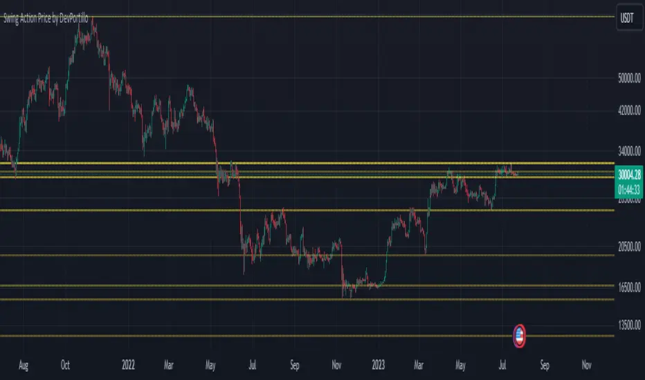
Swing Action PriceEnglish:
**Description of "Swing Action Price" TradingView Script**
"Swing Action Price" is a custom technical indicator designed to identify swing highs and swing lows in a financial market. The script calculates and plots various lines on the chart to visualize these swing points. Swing highs are points where the price has made a local peak, while swing lows are points where the price has made a local trough.
The indicator displays the following lines on the chart:
1. Dotted lines representing each individual swing high and swing low identified on different timeframes (10, 30, 60, 100, 150, 200, 700, and 1000 bars).
2. Dotted lines representing the most recent swing high and swing low for the current bar.
How the indicator works:
1. The script uses historical price data to calculate swing highs and swing lows based on specific conditions.
2. For each of the mentioned timeframes, the indicator identifies the highest high and lowest low within a defined number of bars (10, 30, 60, etc.).
3. Once a new swing high or swing low is identified, the corresponding dotted lines are drawn on the chart, extending from the previous swing point to the current one.
The "Swing Action Price" indicator can be used by traders to visually identify key support and resistance levels in the market. It helps them recognize potential trend reversals or continuation points, which may be valuable for making trading decisions.
Please note that trading indicators should always be used in conjunction with other technical and fundamental analysis tools to make informed trading choices. The "Swing Action Price" indicator is offered under the Mozilla Public License 2.0, and the developer's username is "damianjorgeportillo."
Remember that past performance is not indicative of future results, and it's essential to exercise caution and apply risk management strategies when trading financial markets.
/******************************/
Spanish:
**Descripción del Script "Swing Action Price" en TradingView**
"Swing Action Price" es un indicador técnico personalizado diseñado para identificar máximos y mínimos en un mercado financiero. El script calcula y muestra diversas líneas en el gráfico para visualizar estos puntos de inflexión. Los máximos se producen cuando el precio alcanza un pico local, mientras que los mínimos ocurren cuando el precio alcanza un valle local.
El indicador muestra las siguientes líneas en el gráfico:
1. Líneas punteadas que representan cada máximo y mínimo individual identificado en diferentes marcos de tiempo (10, 30, 60, 100, 150, 200, 700 y 1000 barras).
2. Líneas punteadas que representan el máximo y mínimo más reciente para la barra actual.
Cómo funciona el indicador:
1. El script utiliza datos históricos de precios para calcular los máximos y mínimos en función de ciertas condiciones.
2. Para cada uno de los marcos de tiempo mencionados, el indicador identifica el máximo más alto y el mínimo más bajo dentro de un número específico de barras (10, 30, 60, etc.).
3. Una vez que se identifica un nuevo máximo o mínimo, se dibujan las líneas punteadas correspondientes en el gráfico, extendiéndose desde el punto de inflexión anterior hasta el actual.
El indicador "Swing Action Price" puede ser utilizado por traders para identificar visualmente niveles clave de soporte y resistencia en el mercado. Ayuda a reconocer posibles puntos de inversión o continuación de tendencia, lo que puede ser valioso para tomar decisiones comerciales.
Por favor, ten en cuenta que los indicadores de trading siempre deben utilizarse junto con otras herramientas de análisis técnico y fundamental para tomar decisiones comerciales informadas. El indicador "Swing Action Price" se ofrece bajo la Licencia Pública de Mozilla 2.0, y el nombre de usuario del desarrollador es "damianjorgeportillo".
Recuerda que el rendimiento pasado no garantiza resultados futuros, y es esencial ser cauteloso y aplicar estrategias de gestión de riesgos al operar en los mercados financieros.
Risk to Reward - FIXED SL BacktesterDon't know how to code? No problem! TradingView is an excellent platform for you. ✅ ✅
If you have an indicator that you want to backtest using a risk-to-reward ratio or fixed take profit/stop loss levels, then the Risk to Reward - FIXED SL Backtester script is the perfect solution for you.
introducing Risk to Reward - FIXED SL Backtester Script which will allow you to test any indicator / Signal with RR or Fixed SL system
How does it work ?!
Once you connect the script to your indicator, it will analyze your entry points and perform calculations based on them. It will then open trades for you according to the specified inputs in the script settings.
HOW TO CONNECT IT to your indicator?
simply open your indicator code and add the below line of code to it
plot(Signal ? 100 : 0,"Signal",display = display.data_window)
Replace Signal with the long condition from your own indicator. You can also modify the value 100 to any number you prefer. After that, open the settings.
Once the script is connected to your indicator, you can choose from two options:
Risk To Reward Ratio System
Fixed TP/ SL System
🔸if you select the Risk to Reward System ⤵️
The Risk-to-Reward System requires the calculation of a stop loss. That's why I have included three different types of stop-loss calculations for you to choose from:
ATR Based SL
Pivot Low SL
VWAP Based SL
Your stop loss and take profit levels will be automatically calculated based on the selected stop loss method and your risk-to-reward ratio.
You can also adjust their values to match your desired risk level. The trades will be displayed on the chart.
with the ability to change their values to match your risk.
once this is done, trades will be displayed on the chart
🔸if you select the Fixed system ⤵️
You have 2 inputs, which are FIXED TP & Fixed SL
input the values you want, and trades will be on your chart...
I have also added a Breakeven feature for you.
with this Breakeven feature the trade will not just move SL to Entry ?! NO NO, it will place it above entry by a % you input yourself, so you always win! 🚀
Here is an example
Enjoy, and have fun, if you have any questions do not hesitate to ask

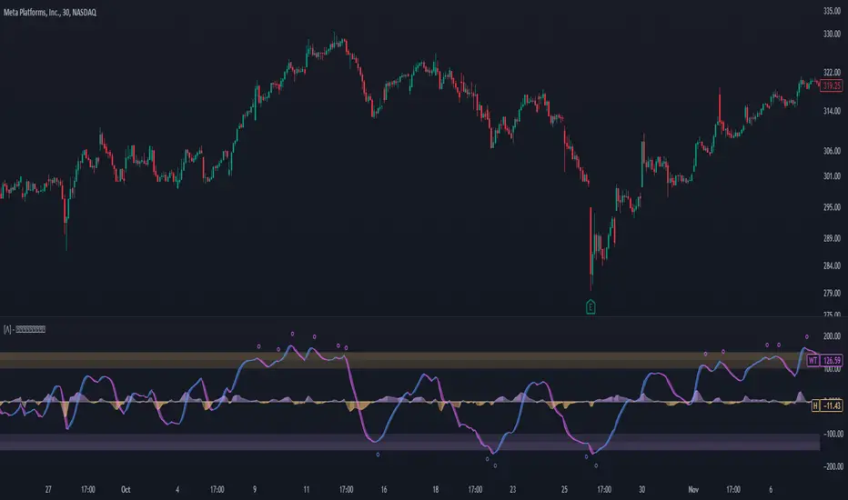
Enhanced WaveTrend OscillatorThe Enhanced WaveTrend Oscillator is a modified version of the original WaveTrend. The WaveTrend indicator is a popular technical analysis tool used to identify overbought and oversold conditions in the market and generate trading signals. The enhanced version addresses certain limitations of the original indicator and introduces additional features for improved analysis and comparison across assets.
WaveTrend:
The original WaveTrend indicator calculates two lines based on exponential moving averages and their relationship to the asset's price. The first line measures the distance between the asset's price and its EMA, while the second line smooths the first line over a specific period. The result is divided by 0.015 multiplied by the smoothed difference ('d' for reference). The indicator aims to identify overbought and oversold conditions by analyzing the relationship between the two lines.
In the original formula, the rudimentary estimation factor 0.015 times 'd' fails to accomodate for approximately a quarter of the data, preventing the indicator from reaching the traditional stationary levels of +-100. This limitation renders the indicator quantitatively biased, as it relies on the user's subjective adjustment of the levels. The enhanced version replaces this factor with the standard deviation of the asset's price, resulting in improved estimation accuracy and provides a more dynamic and robust outcome, we thereafter multiply the result by 100 to achieve a more traditional oscillation.
Enhancements and Features:
The enhanced version of the WaveTrend indicator addresses several limitations of the original indicator and introduces additional features-
Dynamic Estimation: The original indicator uses an arbitrary estimation factor, while the enhanced version replaces it with the standard deviation of the asset's price. This modification provides a more dynamic and accurate estimation, adapting to the specific price characteristics of each asset.
Stationary Support and Resistance Levels: The enhanced version provides stationary key support and resistance levels that range from -150 to 150. These levels are determined based on the analysis of the indicator's data and encompass more than 95% of the indicator's values. These levels offer important reference points for traders to identify potential price reversals or significant price movements.
Comparison Across Assets: The enhanced version allows for better comparison and analysis across different assets. By incorporating the standard deviation of the asset's price, the indicator provides a more consistent and comparable interpretation of the market conditions across multiple assets.
Upon closer inspection of the modification in the enhanced version, we can observe that the resulting indicator is a smoothed variation of the Z-Score!
f_ewave(src, chlen, avglen) =>
basis = ta.ema(src, chlen)
dev = ta.stdev(src, chlen)
wave = (src - basis) / dev * 100
ta.ema(wave, avglen)
Z-Score Analysis:
The Z-Score is a statistical measurement that quantifies how far a particular data point deviates from the mean in terms of standard deviations. In the enhanced version, the calculation involves determining the basis (mean) and deviation (standard deviation) of the asset's price to calculate its Z-Score, thereafter applying a smoothing technique to generate the final WaveTrend value.
Utility:
The 𝗘𝗻𝗵𝗮𝗻𝗰𝗲𝗱 𝗪𝗧 indicator offers traders and investors valuable insights into overbought and oversold conditions in the market. By analyzing the indicator's values and referencing the stationary support and resistance levels, traders can identify potential trend reversals, evaluate market strength, and make better informed analysis.
It is important to note that this indicator should be used in conjunction with other technical analysis tools and indicators to confirm trading signals and validate market dynamics.
Credit:
The 𝗘𝗻𝗵𝗮𝗻𝗰𝗲𝗱 𝗪𝗧 indicator is a modification of the original WaveTrend Oscillator developed by @LazyBear on TradingView.
Example Charts:
Discrete Fourier Transformed Money Flow IndexThe Discrete Fourier Transform Money Flow Index indicator integrates the Money Flow Index (MFI) with Discrete Fourier Transform (credit to author wbburgin - May 26 2023 ) smoothing to offer a refined and smoothed depiction of the MFI's underlying trend. The MFI is calculated using the formula: MFI = 100 - (100 / (1 + MR)), where a high MFI value indicates robust buying pressure (signaling an overbought condition), and a low MFI value indicates substantial selling pressure (signaling an oversold condition).
Why is the DFT and MFI combined?
The aim of this combination between DFT and MFI is to effectively filter out short-term fluctuations and noise, enabling a clearer assessment of the overall trend. This smoothing process enhances the reliability of the MFI by emphasizing dominant and sustained buying or selling pressures. This script executes a full DFT but only uses filtering from one frequency component. The choice to focus on the magnitude at index 0 is significant as it captures the dominant or fundamental frequency in the data. By analyzing this primary cyclic behavior, we can identify recurring patterns and potential turning points more easily. This streamlined approach simplifies interpretation and enhances efficiency by reducing complexity associated with multiple frequency components. Overall, focusing on the dominant frequency and applying it to the MFI provides a concise and actionable assessment of the underlying data.
Note: The FMFI indicator provides both smoothed and non-smoothed versions of the MFI, with the option to toggle the original non-smoothed MFI on or off in the settings.
Application
FMFI functions as a trend-following indicator. Bullish trends are denoted by the color white, while bearish trends are represented by the color purple. Circles plotted on the FMFI indicate regular bull and bear signals. Additionally, red arrows indicate a strong negative trend, while green arrows indicate a strong positive trend. These arrows are calculated based on the presence of regular bull and bear signals within overbought and oversold zones. To enhance its effectiveness, it is recommended to combine this indicator with other complementary technical analysis tools and integrate it into a comprehensive trading strategy. Traders are encouraged to explore a wide range of settings and timeframes to align the indicator with their unique trading preferences and adapt it to the current market conditions. By doing so, traders can optimize the indicator's performance and increase their potential for successful trading outcomes.
Utility
Traders and investors can employ this indicator to enhance their trend-following strategies. The white-colored components of the FMFI can help identify potential buying zones, while the purple-colored components can assist in identifying potential selling points. The red and green arrows can be used to pinpoint moments of strong bull or bear momentum, allowing traders to position themselves advantageously in their trading activities. Please note that future performance of any trading strategy is fundamentally unknowable, and past results do not guarantee future performance.

Trend Correlation HeatmapHello everyone!
I am excited to release my trend correlation heatmap, or trend heatmap for short.
Per usual, I think its important to explain the theory before we get into the use of the indicator, so let's get into the theory!
The theory:
So what is a correlation?
Correlation is the relationship one variable has to another. Correlations are the basis of everything I do as a quantitative trader. From the correlation between the same variables (i.e. autocorrelation), the correlation between other variables (i.e. VIX and SPY, SPY High and SPY Low, DXY and ES1! close, etc.) and, as well, the correlation between price and time (time series correlation).
This may sound very familiar to you, especially if you are a user, observer or follower of my ideas and/or indicators. Ninety-five percent of my indicators are a function of one of those three things. Whether it be a time series based indicator (i.e.my time series indicator), whether it be autocorrelation (my autoregressive cloud indicator or my autocorrelation oscillator) or whether it be regressive in nature (i.e. my SPY Volume weighted close, or even my expected move which uses averages in lieu of regressive approaches but is foundational in regression principles. Or even my VIX oscillator which relies on the premise of correlations between tickers.) So correlation is extremely important to me and while its true I am more of a regression trader than anything, I would argue that I am more of a correlation trader, because correlations are the backbone of how I develop math models of stocks.
What I am trying to stress here is the importance of correlations. They really truly are foundational to any type of quantitative analysis for stocks. And as such, understanding the current relationship a stock has to time is pivotal for any meaningful analysis to be conducted.
So what is correlation to time and what does it tell us?
Correlation to time, otherwise known and commonly referred to as "Time Series", is the relationship a ticker's price has to the passing of time. It is displayed in the traditional Pearson Correlation Coefficient or R value and can be any value from -1 (strong negative relationship, i.e. a strong downtrend) to + 1 (i.e. a strong positive relationship, i.e. a strong uptrend). The higher or lower the value the stronger the up or downtrend is.
As such, correlation to time tells us two very important things. These are:
a) The direction of the stock; and
b) The strength of the trend.
Let's take a look at an example:
Above we have a chart of QQQ. We can see a trendline that seems to fit well. The questions we ask as traders are:
1. What is the likelihood QQQ breaks down from this trendline?
2. What is the likelihood QQQ continues up?
3. What is the likelihood QQQ does a false breakdown?
There are numerous mathematical approaches we can take to answer these questions. For example, 1 and 2 can be answered by use of a Cumulative Distribution Density analysis (CDDA) or even a linear or loglinear regression analysis and 3 can be answered, more or less, with a linear regression analysis and standard error ascertainment, or even just a general comparison using a data science approach (such as cosine similarity or Manhattan distance).
But, the reality is, all 3 of these questions can be visualized, at least in some way, by simply looking at the correlation to time. Let's look at this chart again, this time with the correlation heatmap applied:
If we look at the indicator we can see some pivotal things. These are:
1. We have 4, very strong uptrends that span both higher AND lower timeframes. We have a strong uptrend of 0.96 on the 5 minute, 50 candle period. We have a strong uptrend at the 300 candle lookback period on the 1 minute, we have a strong uptrend on the 100 day lookback on the daily timeframe period and we have a strong uptrend on the 5 minute on the 500 candle lookback period.
2. By comparison, we have 3 downtrends, all of which have correlations less than the 4 uptrends. All of the downtrends have a correlation above -0.8 (which we would want lower than -0.8 to be very strong), and all of the uptrends are greater than + 0.80.
3. We can also see that the uptrends are not confined to the smaller timeframes. We have multiple uptrends on multiple timeframes and both short term (50 to 100 candles) and long term (up to 500 candles).
4. The overall trend is strengthening to the upside manifested by a positive Max Change and a Positive Min change (to be discussed later more in-depth).
With this, we can see that QQQ is actually very strong and likely will continue at least some upside. If we let this play out:
We continued up, had one test and then bounced.
Now, I want to specify, this indicator is not a panacea for all trading. And in relation to the 3 questions posed, they are best answered, at least quantitatively, not only by correlation but also by the aforementioned methods (CDDA, etc.) but correlation will help you get a feel for the strength or weakness present with a stock.
What are some tangible applications of the indicator?
For me, this indicator is used in many ways. Let me outline some ways I generally apply this indicator in my day and swing trading:
1. Gauging the strength of the stock: The indictor tells you the most prevalent behavior of the stock. Are there more downtrends than uptrends present? Are the downtrends present on the larger timeframes vs uptrends on the shorter indicating a possible bullish reversal? or vice versa? Are the trends strengthening or weakening? All of these things can be visualized with the indicator.
2. Setting parameters for other indicators: If you trade EMAs or SMAs, you may have a "one size fits all" approach. However, its actually better to adjust your EMA or SMA length to the actual trend itself. Take a look at this:
This is QQQ on the 1 hour with the 200 EMA with 200 standard deviation bands added. If we look at the heatmap, we can see, yes indeed 200 has a fairly strong uptrend correlation of 0.70. But the strongest hourly uptrend is actually at 400 candles, with a correlation of 0.91. So what happens if we change the EMA length and standard deviation to 400? This:
The exact areas are circled and colour coded. You can see, the 400 offers more of a better reference point of supports and resistances as well as a better overall trend fit. And this is why I never advocate for getting married to a specific EMA. If you are an EMA 200 lover or 21 or 51, know that these are not always the best depending on the trend and situation.
Components of the indicator:
Ah okay, now for the boring stuff. Let's go over the functionality of the indicator. I tried to keep it simple, so it is pretty straight forward. If we open the menu here are our options:
We have the ability to toggle whichever timeframes we want. We also have the ability to toggle on or off the legend that displays the colour codes and the Max and Min highest change.
Max and Min highest change: The max and min highest change simply display the change in correlation over the previous 14 candles. An increasing Max change means that the Max trend is strengthening. If we see an increasing Max change and an increasing Min change (the Min correlation is moving up), this means the stock is bullish. Why? Because the min (i.e. ideally a big negative number) is going up closer to the positives. Therefore, the downtrend is weakening.
If we see both the Max and Min declining (red), that means the uptrend is weakening and downtrend is strengthening. Here are some examples:
Final Thoughts:
And that is the indicator and the theory behind the indicator.
In a nutshell, to summarize, the indicator simply tracks the correlation of a ticker to time on multiple timeframes. This will allow you to make judgements about strength, sentiment and also help you adjust which tools and timeframes you are using to perform your analyses.
As well, to make the indicator more user friendly, I tried to make the colours distinctively different. I was going to do different shades but it was a little difficult to visualize. As such, I have included a toggle-able legend with a breakdown of the colour codes!
That's it my friends, I hope you find it useful!
Safe trades and leave your questions, comments and feedback below!

The Z-score The Z-score, also known as the standard score, is a statistical measurement that describes a value's relationship to the mean of a group of values. It's measured in terms of standard deviations from the mean. If a Z-score is 0, it indicates that the data point's score is identical to the mean score. Z-scores may be positive or negative, with a positive value indicating the score is above the mean and a negative score indicating it is below the mean.
The concept of Z-score was introduced by statistician Carl Friedrich Gauss as part of his "method of the least squares," which was an important step in the development of the normal distribution and Z-score tables. It's a key concept in statistics and is used in various statistical tests.
In financial analysis, Z-scores are used to determine whether a data point is usual or unusual. You can think of it as a measure of how many standard deviations an element is from the mean. For instance, a Z-score of 1.0 would denote a value that is one standard deviation from the mean. Z-scores are also used to predict probabilities, with Z-scores having a distribution that is expected to be normal.
In trading, a Z-score is used to determine how often a trading system may produce a string of winners or losers. It can help a trader to understand whether the losses or profits they see are something that the system would most likely produce, or if it's a once in a blue moon situation. This helps traders make decisions about when to start or stop a system.
I just wanted to play a bit with the Z-score I guess.
Feel free to share your findings if you discover additional applications for this strategy or identify timeframes where it appears to perform more optimally.
How it works:
This strategy is based on a statistical concept called Z-score, which measures the number of standard deviations a data point is from the mean. In other words, it helps determine how unusual or usual a data point is.
In the context of this strategy, Z-score is applied to a 10-period EMA (Exponential Moving Average) of Heikin-Ashi candlestick close prices. The Z-score is calculated over a look-back period of 25 bars.
The EMA of the Z-score is then calculated over a 20-bar period, and the upper and lower thresholds (bounds for buy and sell signals) are defined using the 90th and 10th percentiles of this EMA score.
Long positions are taken when the Z-score crosses above the lower threshold or crosses above the mid-line (50th percentile). An additional long entry is made when the Z-score crosses above the highest value the EMA has been in the past 100 periods.
Short positions are initiated when the EMA crosses below the upper threshold, lower threshold or the highest value the EMA has been in the past 100 periods.
Positions are closed when opposing entry conditions are met, for example, a long position is closed when the short entry condition is true, and vice versa.
Set your desired start date for the strategy. This can be modified in the timestamp("YYYY MM DD") function at the top of the script.

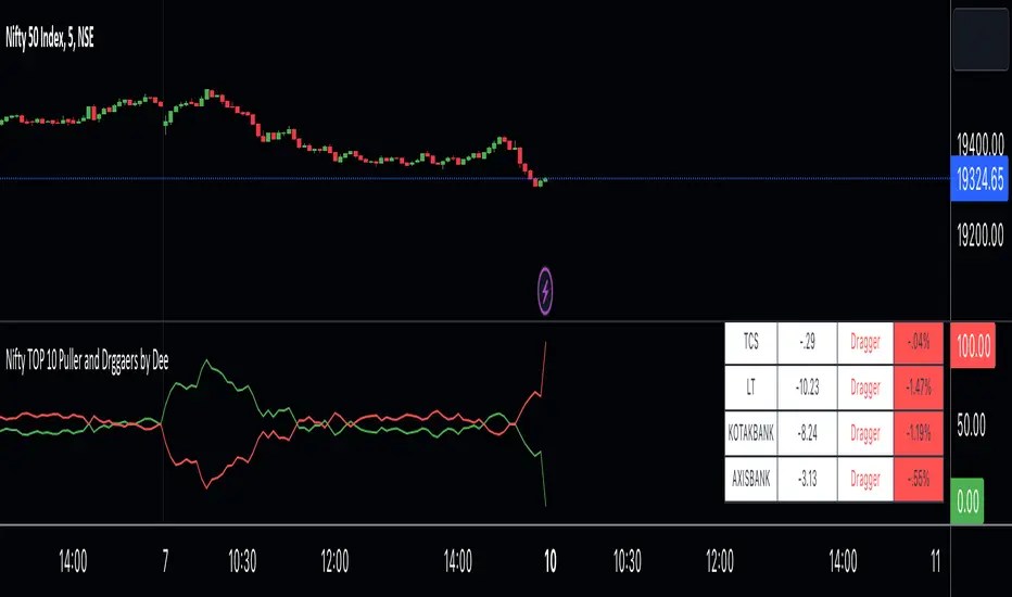
Nifty TOP 10 Puller and Drggaers by Deehi guys this is a straightforward indicator that shows the top 10 nitty pullers and dragger
How to use it ?
in the table, you can see the values of each puller and dragger well as their contribution amount and it will show if they puller or dragger
graph shows the puller and dragger using a line
both have max 100 points allocated
if they exceed the 100 points then a line will struck their ( point to remember ) it does not glitch
so it will give Ruf idea of who is strong
if buyers are strong then the green lien will always be upside
if sellers are string then the red line will always be upside
*Cross Over *
there are 2 types of cross over 1 is bull cross over other is bear cross over
when bulls are strong they will cross over the red from the bottom it showing that significantly strong
when bear is strong they will cross over the green from the bottom it shows that bear is significantly strong
hope you understand how to use it
we have limitation in trading view so we choose only 10 stock to calculate the %
ADW - Volatility MapThe ADW - Volatility Map script is a tool for traders to measure and visualize the volatility of a specific asset. It uses both the Average True Range (ATR) and True Range (TR) values in combination with the Commodity Channel Index (CCI) to provide a comprehensive map of the market's volatility.
Average True Range (ATR) : ATR is a measure of market volatility. It measures the average of true price ranges over a time period. In this script, we use it to calculate the ATR-CCI which gives us a more precise measure of volatility.
True Range (TR) : TR is the greatest distance the price moved during a period. It is used in this script to calculate the TR-CCI, adding another level of detail to our volatility measurement.
Commodity Channel Index (CCI) : CCI is a versatile indicator that can be used to identify a new trend or warn of extreme conditions. We use it to scale and compare the ATR and TR values, hence providing a relative measure of volatility.
The script interprets the CCI values and provides four different conditions for both ATR and TR:
Is Low (CCI < 0)
Is High (CCI > 0)
Is Extremely Low (CCI <= -100)
Is Extremely High (CCI >= 100)
The interpretation of these conditions is displayed on the chart using colour highlighting. When the ATR or TR are low, high, extremely low, or extremely high, the script fills the chart accordingly.
In addition, the script has an option `awaitBarConfirmation` set at the beginning. If this is true, the script will only display indicators for fully formed bars, ensuring that the indicators you see are based on confirmed information.
Note: The colours for different conditions can be customized at the beginning of the script, allowing you to personalize the visual output to match your preferences.
This script is designed to provide a visually clear and immediate understanding of the market's volatility. Use it to enhance your decision-making process and adapt your trading strategy to the current market conditions.

Monthly Gain in percentageThis scripts calculates the percentage gain in a month (previous 22 trade days).
Firstly, it calculates number of sample days
-> minimum no. of sampling duration = 22
-> maximum no. of sampling duration = increased from 22 until 0day_low > 22_day_high
Example if sampling_duration = 100
Monthly percentage gain = ((Current_Day_High_Price - 0_Day_Low_Price) * 100 / 0_Day_Low_Price) * 22 / sampling_duration

Vector3Library "Vector3"
Representation of 3D vectors and points.
This structure is used to pass 3D positions and directions around. It also contains functions for doing common vector operations.
Besides the functions listed below, other classes can be used to manipulate vectors and points as well.
For example the Quaternion and the Matrix4x4 classes are useful for rotating or transforming vectors and points.
___
**Reference:**
- github.com
- github.com
- github.com
- www.movable-type.co.uk
- docs.unity3d.com
- referencesource.microsoft.com
- github.com
\
new(x, y, z)
Create a new `Vector3`.
Parameters:
x (float) : `float` Property `x` value, (optional, default=na).
y (float) : `float` Property `y` value, (optional, default=na).
z (float) : `float` Property `z` value, (optional, default=na).
Returns: `Vector3` Generated new vector.
___
**Usage:**
```
.new(1.1, 1, 1)
```
from(value)
Create a new `Vector3` from a single value.
Parameters:
value (float) : `float` Properties positional value, (optional, default=na).
Returns: `Vector3` Generated new vector.
___
**Usage:**
```
.from(1.1)
```
from_Array(values, fill_na)
Create a new `Vector3` from a list of values, only reads up to the third item.
Parameters:
values (float ) : `array` Vector property values.
fill_na (float) : `float` Parameter value to replace missing indexes, (optional, defualt=na).
Returns: `Vector3` Generated new vector.
___
**Notes:**
- Supports any size of array, fills non available fields with `na`.
___
**Usage:**
```
.from_Array(array.from(1.1, fill_na=33))
.from_Array(array.from(1.1, 2, 3))
```
from_Vector2(values)
Create a new `Vector3` from a `Vector2`.
Parameters:
values (Vector2 type from RicardoSantos/CommonTypesMath/1) : `Vector2` Vector property values.
Returns: `Vector3` Generated new vector.
___
**Usage:**
```
.from:Vector2(.Vector2.new(1, 2.0))
```
___
**Notes:**
- Type `Vector2` from CommonTypesMath library.
from_Quaternion(values)
Create a new `Vector3` from a `Quaternion`'s `x, y, z` properties.
Parameters:
values (Quaternion type from RicardoSantos/CommonTypesMath/1) : `Quaternion` Vector property values.
Returns: `Vector3` Generated new vector.
___
**Usage:**
```
.from_Quaternion(.Quaternion.new(1, 2, 3, 4))
```
___
**Notes:**
- Type `Quaternion` from CommonTypesMath library.
from_String(expression, separator, fill_na)
Create a new `Vector3` from a list of values in a formated string.
Parameters:
expression (string) : `array` String with the list of vector properties.
separator (string) : `string` Separator between entries, (optional, default=`","`).
fill_na (float) : `float` Parameter value to replace missing indexes, (optional, defualt=na).
Returns: `Vector3` Generated new vector.
___
**Notes:**
- Supports any size of array, fills non available fields with `na`.
- `",,"` Empty fields will be ignored.
___
**Usage:**
```
.from_String("1.1", fill_na=33))
.from_String("(1.1,, 3)") // 1.1 , 3.0, NaN // empty field will be ignored!!
```
back()
Create a new `Vector3` object in the form `(0, 0, -1)`.
Returns: `Vector3` Generated new vector.
___
**Usage:**
```
.back()
```
front()
Create a new `Vector3` object in the form `(0, 0, 1)`.
Returns: `Vector3` Generated new vector.
___
**Usage:**
```
.front()
```
up()
Create a new `Vector3` object in the form `(0, 1, 0)`.
Returns: `Vector3` Generated new vector.
___
**Usage:**
```
.up()
```
down()
Create a new `Vector3` object in the form `(0, -1, 0)`.
Returns: `Vector3` Generated new vector.
___
**Usage:**
```
.down()
```
left()
Create a new `Vector3` object in the form `(-1, 0, 0)`.
Returns: `Vector3` Generated new vector.
___
**Usage:**
```
.left()
```
right()
Create a new `Vector3` object in the form `(1, 0, 0)`.
Returns: `Vector3` Generated new vector.
___
**Usage:**
```
.right()
```
zero()
Create a new `Vector3` object in the form `(0, 0, 0)`.
Returns: `Vector3` Generated new vector.
___
**Usage:**
```
.zero()
```
one()
Create a new `Vector3` object in the form `(1, 1, 1)`.
Returns: `Vector3` Generated new vector.
___
**Usage:**
```
.one()
```
minus_one()
Create a new `Vector3` object in the form `(-1, -1, -1)`.
Returns: `Vector3` Generated new vector.
___
**Usage:**
```
.minus_one()
```
unit_x()
Create a new `Vector3` object in the form `(1, 0, 0)`.
Returns: `Vector3` Generated new vector.
___
**Usage:**
```
.unit_x()
```
unit_y()
Create a new `Vector3` object in the form `(0, 1, 0)`.
Returns: `Vector3` Generated new vector.
___
**Usage:**
```
.unit_y()
```
unit_z()
Create a new `Vector3` object in the form `(0, 0, 1)`.
Returns: `Vector3` Generated new vector.
___
**Usage:**
```
.unit_z()
```
nan()
Create a new `Vector3` object in the form `(na, na, na)`.
Returns: `Vector3` Generated new vector.
___
**Usage:**
```
.nan()
```
random(max, min)
Generate a vector with random properties.
Parameters:
max (Vector3 type from RicardoSantos/CommonTypesMath/1) : `Vector3` Maximum defined range of the vector properties.
min (Vector3 type from RicardoSantos/CommonTypesMath/1) : `Vector3` Minimum defined range of the vector properties.
Returns: `Vector3` Generated new vector.
___
**Usage:**
```
.random(.from(math.pi), .from(-math.pi))
```
random(max)
Generate a vector with random properties (min set to 0.0).
Parameters:
max (Vector3 type from RicardoSantos/CommonTypesMath/1) : `Vector3` Maximum defined range of the vector properties.
Returns: `Vector3` Generated new vector.
___
**Usage:**
```
.random(.from(math.pi))
```
method copy(this)
Copy a existing `Vector3`
Namespace types: TMath.Vector3
Parameters:
this (Vector3 type from RicardoSantos/CommonTypesMath/1) : `Vector3` Source vector.
Returns: `Vector3` Generated new vector.
___
**Usage:**
```
a = .one().copy()
```
method i_add(this, other)
Modify a instance of a vector by adding a vector to it.
Namespace types: TMath.Vector3
Parameters:
this (Vector3 type from RicardoSantos/CommonTypesMath/1) : `Vector3` Source vector.
other (Vector3 type from RicardoSantos/CommonTypesMath/1) : `Vector3` Other Vector.
Returns: `Vector3` Updated source vector.
___
**Usage:**
```
a = .from(1) , a.i_add(.up())
```
method i_add(this, value)
Modify a instance of a vector by adding a vector to it.
Namespace types: TMath.Vector3
Parameters:
this (Vector3 type from RicardoSantos/CommonTypesMath/1) : `Vector3` Source vector.
value (float) : `float` Value.
Returns: `Vector3` Updated source vector.
___
**Usage:**
```
a = .from(1) , a.i_add(3.2)
```
method i_subtract(this, other)
Modify a instance of a vector by subtracting a vector to it.
Namespace types: TMath.Vector3
Parameters:
this (Vector3 type from RicardoSantos/CommonTypesMath/1) : `Vector3` Source vector.
other (Vector3 type from RicardoSantos/CommonTypesMath/1) : `Vector3` Other Vector.
Returns: `Vector3` Updated source vector.
___
**Usage:**
```
a = .from(1) , a.i_subtract(.down())
```
method i_subtract(this, value)
Modify a instance of a vector by subtracting a vector to it.
Namespace types: TMath.Vector3
Parameters:
this (Vector3 type from RicardoSantos/CommonTypesMath/1) : `Vector3` Source vector.
value (float) : `float` Value.
Returns: `Vector3` Updated source vector.
___
**Usage:**
```
a = .from(1) , a.i_subtract(3)
```
method i_multiply(this, other)
Modify a instance of a vector by multiplying a vector with it.
Namespace types: TMath.Vector3
Parameters:
this (Vector3 type from RicardoSantos/CommonTypesMath/1) : `Vector3` Source vector.
other (Vector3 type from RicardoSantos/CommonTypesMath/1) : `Vector3` Other Vector.
Returns: `Vector3` Updated source vector.
___
**Usage:**
```
a = .from(1) , a.i_multiply(.left())
```
method i_multiply(this, value)
Modify a instance of a vector by multiplying a vector with it.
Namespace types: TMath.Vector3
Parameters:
this (Vector3 type from RicardoSantos/CommonTypesMath/1) : `Vector3` Source vector.
value (float) : `float` value.
Returns: `Vector3` Updated source vector.
___
**Usage:**
```
a = .from(1) , a.i_multiply(3)
```
method i_divide(this, other)
Modify a instance of a vector by dividing it by another vector.
Namespace types: TMath.Vector3
Parameters:
this (Vector3 type from RicardoSantos/CommonTypesMath/1) : `Vector3` Source vector.
other (Vector3 type from RicardoSantos/CommonTypesMath/1) : `Vector3` Other Vector.
Returns: `Vector3` Updated source vector.
___
**Usage:**
```
a = .from(1) , a.i_divide(.forward())
```
method i_divide(this, value)
Modify a instance of a vector by dividing it by another vector.
Namespace types: TMath.Vector3
Parameters:
this (Vector3 type from RicardoSantos/CommonTypesMath/1) : `Vector3` Source vector.
value (float) : `float` Value.
Returns: `Vector3` Updated source vector.
___
**Usage:**
```
a = .from(1) , a.i_divide(3)
```
method i_mod(this, other)
Modify a instance of a vector by modulo assignment with another vector.
Namespace types: TMath.Vector3
Parameters:
this (Vector3 type from RicardoSantos/CommonTypesMath/1) : `Vector3` Source vector.
other (Vector3 type from RicardoSantos/CommonTypesMath/1) : `Vector3` Other Vector.
Returns: `Vector3` Updated source vector.
___
**Usage:**
```
a = .from(1) , a.i_mod(.back())
```
method i_mod(this, value)
Modify a instance of a vector by modulo assignment with another vector.
Namespace types: TMath.Vector3
Parameters:
this (Vector3 type from RicardoSantos/CommonTypesMath/1) : `Vector3` Source vector.
value (float) : `float` Value.
Returns: `Vector3` Updated source vector.
___
**Usage:**
```
a = .from(1) , a.i_mod(3)
```
method i_pow(this, exponent)
Modify a instance of a vector by modulo assignment with another vector.
Namespace types: TMath.Vector3
Parameters:
this (Vector3 type from RicardoSantos/CommonTypesMath/1) : `Vector3` Source vector.
exponent (Vector3 type from RicardoSantos/CommonTypesMath/1) : `Vector3` Exponent Vector.
Returns: `Vector3` Updated source vector.
___
**Usage:**
```
a = .from(1) , a.i_pow(.up())
```
method i_pow(this, exponent)
Modify a instance of a vector by modulo assignment with another vector.
Namespace types: TMath.Vector3
Parameters:
this (Vector3 type from RicardoSantos/CommonTypesMath/1) : `Vector3` Source vector.
exponent (float) : `float` Exponent Value.
Returns: `Vector3` Updated source vector.
___
**Usage:**
```
a = .from(1) , a.i_pow(2)
```
method length_squared(this)
Squared length of the vector.
Namespace types: TMath.Vector3
Parameters:
this (Vector3 type from RicardoSantos/CommonTypesMath/1)
Returns: `float` The squared length of this vector.
___
**Usage:**
```
a = .one().length_squared()
```
method magnitude_squared(this)
Squared magnitude of the vector.
Namespace types: TMath.Vector3
Parameters:
this (Vector3 type from RicardoSantos/CommonTypesMath/1) : `Vector3` Source vector.
Returns: `float` The length squared of this vector.
___
**Usage:**
```
a = .one().magnitude_squared()
```
method length(this)
Length of the vector.
Namespace types: TMath.Vector3
Parameters:
this (Vector3 type from RicardoSantos/CommonTypesMath/1) : `Vector3` Source vector.
Returns: `float` The length of this vector.
___
**Usage:**
```
a = .one().length()
```
method magnitude(this)
Magnitude of the vector.
Namespace types: TMath.Vector3
Parameters:
this (Vector3 type from RicardoSantos/CommonTypesMath/1) : `Vector3` Source vector.
Returns: `float` The Length of this vector.
___
**Usage:**
```
a = .one().magnitude()
```
method normalize(this, magnitude, eps)
Normalize a vector with a magnitude of 1(optional).
Namespace types: TMath.Vector3
Parameters:
this (Vector3 type from RicardoSantos/CommonTypesMath/1) : `Vector3` Source vector.
magnitude (float) : `float` Value to manipulate the magnitude of normalization, (optional, default=1.0).
eps (float)
Returns: `Vector3` Generated new vector.
___
**Usage:**
```
a = .new(33, 50, 100).normalize() // (x=0.283, y=0.429, z=0.858)
a = .new(33, 50, 100).normalize(2) // (x=0.142, y=0.214, z=0.429)
```
method to_String(this, precision)
Converts source vector to a string format, in the form `"(x, y, z)"`.
Namespace types: TMath.Vector3
Parameters:
this (Vector3 type from RicardoSantos/CommonTypesMath/1) : `Vector3` Source vector.
precision (string) : `string` Precision format to apply to values (optional, default='').
Returns: `string` Formated string in a `"(x, y, z)"` format.
___
**Usage:**
```
a = .one().to_String("#.###")
```
method to_Array(this)
Converts source vector to a array format.
Namespace types: TMath.Vector3
Parameters:
this (Vector3 type from RicardoSantos/CommonTypesMath/1) : `Vector3` Source vector.
Returns: `array` List of the vector properties.
___
**Usage:**
```
a = .new(1, 2, 3).to_Array()
```
method to_Vector2(this)
Converts source vector to a Vector2 in the form `x, y`.
Namespace types: TMath.Vector3
Parameters:
this (Vector3 type from RicardoSantos/CommonTypesMath/1) : `Vector3` Source vector.
Returns: `Vector2` Generated new vector.
___
**Usage:**
```
a = .from(1).to_Vector2()
```
method to_Quaternion(this, w)
Converts source vector to a Quaternion in the form `x, y, z, w`.
Namespace types: TMath.Vector3
Parameters:
this (Vector3 type from RicardoSantos/CommonTypesMath/1) : `Vector3` Sorce vector.
w (float) : `float` Property of `w` new value.
Returns: `Quaternion` Generated new vector.
___
**Usage:**
```
a = .from(1).to_Quaternion(w=1)
```
method add(this, other)
Add a vector to source vector.
Namespace types: TMath.Vector3
Parameters:
this (Vector3 type from RicardoSantos/CommonTypesMath/1) : `Vector3` Source vector.
other (Vector3 type from RicardoSantos/CommonTypesMath/1) : `Vector3` Other vector.
Returns: `Vector3` Generated new vector.
___
**Usage:**
```
a = .from(1).add(.unit_z())
```
method add(this, value)
Add a value to each property of the vector.
Namespace types: TMath.Vector3
Parameters:
this (Vector3 type from RicardoSantos/CommonTypesMath/1) : `Vector3` Source vector.
value (float) : `float` Value.
Returns: `Vector3` Generated new vector.
___
**Usage:**
```
a = .from(1).add(2.0)
```
add(value, other)
Add each property of a vector to a base value as a new vector.
Parameters:
value (float) : `float` Value.
other (Vector3 type from RicardoSantos/CommonTypesMath/1) : `Vector3` Vector.
Returns: `Vector3` Generated new vector.
___
**Usage:**
```
a = .from(2) , b = .add(1.0, a)
```
method subtract(this, other)
Subtract vector from source vector.
Namespace types: TMath.Vector3
Parameters:
this (Vector3 type from RicardoSantos/CommonTypesMath/1) : `Vector3` Source vector.
other (Vector3 type from RicardoSantos/CommonTypesMath/1) : `Vector3` Other vector.
Returns: `Vector3` Generated new vector.
___
**Usage:**
```
a = .from(1).subtract(.left())
```
method subtract(this, value)
Subtract a value from each property in source vector.
Namespace types: TMath.Vector3
Parameters:
this (Vector3 type from RicardoSantos/CommonTypesMath/1) : `Vector3` Source vector.
value (float) : `float` Value.
Returns: `Vector3` Generated new vector.
___
**Usage:**
```
a = .from(1).subtract(2.0)
```
subtract(value, other)
Subtract each property in a vector from a base value and create a new vector.
Parameters:
value (float) : `float` Value.
other (Vector3 type from RicardoSantos/CommonTypesMath/1) : `Vector3` Vector.
Returns: `Vector3` Generated new vector.
___
**Usage:**
```
a = .subtract(1.0, .right())
```
method multiply(this, other)
Multiply a vector by another.
Namespace types: TMath.Vector3
Parameters:
this (Vector3 type from RicardoSantos/CommonTypesMath/1) : `Vector3` Source vector.
other (Vector3 type from RicardoSantos/CommonTypesMath/1) : `Vector3` Other vector.
Returns: `Vector3` Generated new vector.
___
**Usage:**
```
a = .from(1).multiply(.up())
```
method multiply(this, value)
Multiply each element in source vector with a value.
Namespace types: TMath.Vector3
Parameters:
this (Vector3 type from RicardoSantos/CommonTypesMath/1) : `Vector3` Source vector.
value (float) : `float` Value.
Returns: `Vector3` Generated new vector.
___
**Usage:**
```
a = .from(1).multiply(2.0)
```
multiply(value, other)
Multiply a value with each property in a vector and create a new vector.
Parameters:
value (float) : `float` Value.
other (Vector3 type from RicardoSantos/CommonTypesMath/1) : `Vector3` Vector.
Returns: `Vector3` Generated new vector.
___
**Usage:**
```
a = .multiply(1.0, .new(1, 2, 1))
```
method divide(this, other)
Divide a vector by another.
Namespace types: TMath.Vector3
Parameters:
this (Vector3 type from RicardoSantos/CommonTypesMath/1) : `Vector3` Source vector.
other (Vector3 type from RicardoSantos/CommonTypesMath/1) : `Vector3` Other vector.
Returns: `Vector3` Generated new vector.
___
**Usage:**
```
a = .from(1).divide(.from(2))
```
method divide(this, value)
Divide each property in a vector by a value.
Namespace types: TMath.Vector3
Parameters:
this (Vector3 type from RicardoSantos/CommonTypesMath/1) : `Vector3` Source vector.
value (float) : `float` Value.
Returns: `Vector3` Generated new vector.
___
**Usage:**
```
a = .from(1).divide(2.0)
```
divide(value, other)
Divide a base value by each property in a vector and create a new vector.
Parameters:
value (float) : `float` Value.
other (Vector3 type from RicardoSantos/CommonTypesMath/1) : `Vector3` Vector.
Returns: `Vector3` Generated new vector.
___
**Usage:**
```
a = .divide(1.0, .from(2))
```
method mod(this, other)
Modulo a vector by another.
Namespace types: TMath.Vector3
Parameters:
this (Vector3 type from RicardoSantos/CommonTypesMath/1) : `Vector3` Source vector.
other (Vector3 type from RicardoSantos/CommonTypesMath/1) : `Vector3` Other vector.
Returns: `Vector3` Generated new vector.
___
**Usage:**
```
a = .from(1).mod(.from(2))
```
method mod(this, value)
Modulo each property in a vector by a value.
Namespace types: TMath.Vector3
Parameters:
this (Vector3 type from RicardoSantos/CommonTypesMath/1) : `Vector3` Source vector.
value (float) : `float` Value.
Returns: `Vector3` Generated new vector.
___
**Usage:**
```
a = .from(1).mod(2.0)
```
mod(value, other)
Modulo a base value by each property in a vector and create a new vector.
Parameters:
value (float) : `float` Value.
other (Vector3 type from RicardoSantos/CommonTypesMath/1) : `Vector3` Vector.
Returns: `Vector3` Generated new vector.
___
**Usage:**
```
a = .mod(1.0, .from(2))
```
method negate(this)
Negate a vector in the form `(zero - this)`.
Namespace types: TMath.Vector3
Parameters:
this (Vector3 type from RicardoSantos/CommonTypesMath/1) : `Vector3` Source vector.
Returns: `Vector3` Generated new vector.
___
**Usage:**
```
a = .one().negate()
```
method pow(this, other)
Modulo a vector by another.
Namespace types: TMath.Vector3
Parameters:
this (Vector3 type from RicardoSantos/CommonTypesMath/1) : `Vector3` Source vector.
other (Vector3 type from RicardoSantos/CommonTypesMath/1) : `Vector3` Other vector.
Returns: `Vector3` Generated new vector.
___
**Usage:**
```
a = .from(2).pow(.from(3))
```
method pow(this, exponent)
Raise the vector elements by a exponent.
Namespace types: TMath.Vector3
Parameters:
this (Vector3 type from RicardoSantos/CommonTypesMath/1) : `Vector3` Source vector.
exponent (float) : `float` The exponent to raise the vector by.
Returns: `Vector3` Generated new vector.
___
**Usage:**
```
a = .from(1).pow(2.0)
```
pow(value, exponent)
Raise value into a vector raised by the elements in exponent vector.
Parameters:
value (float) : `float` Base value.
exponent (Vector3 type from RicardoSantos/CommonTypesMath/1) : `Vector3` The exponent to raise the vector of base value by.
Returns: `Vector3` Generated new vector.
___
**Usage:**
```
a = .pow(1.0, .from(2))
```
method sqrt(this)
Square root of the elements in a vector.
Namespace types: TMath.Vector3
Parameters:
this (Vector3 type from RicardoSantos/CommonTypesMath/1) : `Vector3` Source vector.
Returns: `Vector3` Generated new vector.
___
**Usage:**
```
a = .from(1).sqrt()
```
method abs(this)
Absolute properties of the vector.
Namespace types: TMath.Vector3
Parameters:
this (Vector3 type from RicardoSantos/CommonTypesMath/1) : `Vector3` Source vector.
Returns: `Vector3` Generated new vector.
___
**Usage:**
```
a = .from(1).abs()
```
method max(this)
Highest property of the vector.
Namespace types: TMath.Vector3
Parameters:
this (Vector3 type from RicardoSantos/CommonTypesMath/1) : `Vector3` Source vector.
Returns: `float` Highest value amongst the vector properties.
___
**Usage:**
```
a = .new(1, 2, 3).max()
```
method min(this)
Lowest element of the vector.
Namespace types: TMath.Vector3
Parameters:
this (Vector3 type from RicardoSantos/CommonTypesMath/1) : `Vector3` Source vector.
Returns: `float` Lowest values amongst the vector properties.
___
**Usage:**
```
a = .new(1, 2, 3).min()
```
method floor(this)
Floor of vector a.
Namespace types: TMath.Vector3
Parameters:
this (Vector3 type from RicardoSantos/CommonTypesMath/1) : `Vector3` Source vector.
Returns: `Vector3` Generated new vector.
___
**Usage:**
```
a = .new(1.33, 1.66, 1.99).floor()
```
method ceil(this)
Ceil of vector a.
Namespace types: TMath.Vector3
Parameters:
this (Vector3 type from RicardoSantos/CommonTypesMath/1) : `Vector3` Source vector.
Returns: `Vector3` Generated new vector.
___
**Usage:**
```
a = .new(1.33, 1.66, 1.99).ceil()
```
method round(this)
Round of vector elements.
Namespace types: TMath.Vector3
Parameters:
this (Vector3 type from RicardoSantos/CommonTypesMath/1) : `Vector3` Source vector.
Returns: `Vector3` Generated new vector.
___
**Usage:**
```
a = .new(1.33, 1.66, 1.99).round()
```
method round(this, precision)
Round of vector elements to n digits.
Namespace types: TMath.Vector3
Parameters:
this (Vector3 type from RicardoSantos/CommonTypesMath/1) : `Vector3` Source vector.
precision (int) : `int` Number of digits to round the vector elements.
Returns: `Vector3` Generated new vector.
___
**Usage:**
```
a = .new(1.33, 1.66, 1.99).round(1) // 1.3, 1.7, 2
```
method fractional(this)
Fractional parts of vector.
Namespace types: TMath.Vector3
Parameters:
this (Vector3 type from RicardoSantos/CommonTypesMath/1) : `Vector3` Source vector.
Returns: `Vector3` Generated new vector.
___
**Usage:**
```
a = .from(1.337).fractional() // 0.337
```
method dot_product(this, other)
Dot product of two vectors.
Namespace types: TMath.Vector3
Parameters:
this (Vector3 type from RicardoSantos/CommonTypesMath/1) : `Vector3` Source vector.
other (Vector3 type from RicardoSantos/CommonTypesMath/1) : `Vector3` Other vector.
Returns: `float` Dot product.
___
**Usage:**
```
a = .from(2).dot_product(.left())
```
method cross_product(this, other)
Cross product of two vectors.
Namespace types: TMath.Vector3
Parameters:
this (Vector3 type from RicardoSantos/CommonTypesMath/1) : `Vector3` Source vector.
other (Vector3 type from RicardoSantos/CommonTypesMath/1) : `Vector3` Other vector.
Returns: `Vector3` Generated new vector.
___
**Usage:**
```
a = .from(1).cross_produc(.right())
```
method scale(this, scalar)
Scale vector by a scalar value.
Namespace types: TMath.Vector3
Parameters:
this (Vector3 type from RicardoSantos/CommonTypesMath/1) : `Vector3` Source vector.
scalar (float) : `float` Value to scale the the vector by.
Returns: `Vector3` Generated new vector.
___
**Usage:**
```
a = .from(1).scale(2)
```
method rescale(this, magnitude)
Rescale a vector to a new magnitude.
Namespace types: TMath.Vector3
Parameters:
this (Vector3 type from RicardoSantos/CommonTypesMath/1) : `Vector3` Source vector.
magnitude (float) : `float` Value to manipulate the magnitude of normalization.
Returns: `Vector3` Generated new vector.
___
**Usage:**
```
a = .from(20).rescale(1)
```
method equals(this, other)
Compares two vectors.
Namespace types: TMath.Vector3
Parameters:
this (Vector3 type from RicardoSantos/CommonTypesMath/1) : `Vector3` Source vector.
other (Vector3 type from RicardoSantos/CommonTypesMath/1) : `Vector3` Other vector.
Returns: `Vector3` Generated new vector.
___
**Usage:**
```
a = .from(1).equals(.one())
```
method sin(this)
Sine of vector.
Namespace types: TMath.Vector3
Parameters:
this (Vector3 type from RicardoSantos/CommonTypesMath/1) : `Vector3` Source vector.
Returns: `Vector3` Generated new vector.
___
**Usage:**
```
a = .from(1).sin()
```
method cos(this)
Cosine of vector.
Namespace types: TMath.Vector3
Parameters:
this (Vector3 type from RicardoSantos/CommonTypesMath/1) : `Vector3` Source vector.
Returns: `Vector3` Generated new vector.
___
**Usage:**
```
a = .from(1).cos()
```
method tan(this)
Tangent of vector.
Namespace types: TMath.Vector3
Parameters:
this (Vector3 type from RicardoSantos/CommonTypesMath/1) : `Vector3` Source vector.
Returns: `Vector3` Generated new vector.
___
**Usage:**
```
a = .from(1).tan()
```
vmax(a, b)
Highest elements of the properties from two vectors.
Parameters:
a (Vector3 type from RicardoSantos/CommonTypesMath/1) : `Vector3` Vector.
b (Vector3 type from RicardoSantos/CommonTypesMath/1) : `Vector3` Vector.
Returns: `Vector3` Generated new vector.
___
**Usage:**
```
a = .vmax(.one(), .from(2))
```
vmax(a, b, c)
Highest elements of the properties from three vectors.
Parameters:
a (Vector3 type from RicardoSantos/CommonTypesMath/1) : `Vector3` Vector.
b (Vector3 type from RicardoSantos/CommonTypesMath/1) : `Vector3` Vector.
c (Vector3 type from RicardoSantos/CommonTypesMath/1) : `Vector3` Vector.
Returns: `Vector3` Generated new vector.
___
**Usage:**
```
a = .vmax(.new(0.1, 2.5, 3.4), .from(2), .from(3))
```
vmin(a, b)
Lowest elements of the properties from two vectors.
Parameters:
a (Vector3 type from RicardoSantos/CommonTypesMath/1) : `Vector3` Vector.
b (Vector3 type from RicardoSantos/CommonTypesMath/1) : `Vector3` Vector.
Returns: `Vector3` Generated new vector.
___
**Usage:**
```
a = .vmin(.one(), .from(2))
```
vmin(a, b, c)
Lowest elements of the properties from three vectors.
Parameters:
a (Vector3 type from RicardoSantos/CommonTypesMath/1) : `Vector3` Vector.
b (Vector3 type from RicardoSantos/CommonTypesMath/1) : `Vector3` Vector.
c (Vector3 type from RicardoSantos/CommonTypesMath/1) : `Vector3` Vector.
Returns: `Vector3` Generated new vector.
___
**Usage:**
```
a = .vmin(.one(), .from(2), .new(3.3, 2.2, 0.5))
```
distance(a, b)
Distance between vector `a` and `b`.
Parameters:
a (Vector3 type from RicardoSantos/CommonTypesMath/1) : `Vector3` Source vector.
b (Vector3 type from RicardoSantos/CommonTypesMath/1) : `Vector3` Target vector.
Returns: `Vector3` Generated new vector.
___
**Usage:**
```
a = distance(.from(3), .unit_z())
```
clamp(a, min, max)
Restrict a vector between a min and max vector.
Parameters:
a (Vector3 type from RicardoSantos/CommonTypesMath/1) : `Vector3` Source vector.
min (Vector3 type from RicardoSantos/CommonTypesMath/1) : `Vector3` Minimum boundary vector.
max (Vector3 type from RicardoSantos/CommonTypesMath/1) : `Vector3` Maximum boundary vector.
Returns: `Vector3` Generated new vector.
___
**Usage:**
```
a = .clamp(a=.new(2.9, 1.5, 3.9), min=.from(2), max=.new(2.5, 3.0, 3.5))
```
clamp_magnitude(a, radius)
Vector with its magnitude clamped to a radius.
Parameters:
a (Vector3 type from RicardoSantos/CommonTypesMath/1) : `Vector3` Source vector.object, vector with properties that should be restricted to a radius.
radius (float) : `float` Maximum radius to restrict magnitude of vector.
Returns: `Vector3` Generated new vector.
___
**Usage:**
```
a = .clamp_magnitude(.from(21), 7)
```
lerp_unclamped(a, b, rate)
`Unclamped` linearly interpolates between provided vectors by a rate.
Parameters:
a (Vector3 type from RicardoSantos/CommonTypesMath/1) : `Vector3` Source vector.
b (Vector3 type from RicardoSantos/CommonTypesMath/1) : `Vector3` Target vector.
rate (float) : `float` Rate of interpolation, range(0 > 1) where 0 == source vector and 1 == target vector.
Returns: `Vector3` Generated new vector.
___
**Usage:**
```
a = .lerp_unclamped(.from(1), .from(2), 1.2)
```
lerp(a, b, rate)
Linearly interpolates between provided vectors by a rate.
Parameters:
a (Vector3 type from RicardoSantos/CommonTypesMath/1) : `Vector3` Source vector.
b (Vector3 type from RicardoSantos/CommonTypesMath/1) : `Vector3` Target vector.
rate (float) : `float` Rate of interpolation, range(0 > 1) where 0 == source vector and 1 == target vector.
Returns: `Vector3` Generated new vector.
___
**Usage:**
```
a = lerp(.one(), .from(2), 0.2)
```
herp(start, start_tangent, end, end_tangent, rate)
Hermite curve interpolation between provided vectors.
Parameters:
start (Vector3 type from RicardoSantos/CommonTypesMath/1) : `Vector3` Start vector.
start_tangent (Vector3 type from RicardoSantos/CommonTypesMath/1) : `Vector3` Start vector tangent.
end (Vector3 type from RicardoSantos/CommonTypesMath/1) : `Vector3` End vector.
end_tangent (Vector3 type from RicardoSantos/CommonTypesMath/1) : `Vector3` End vector tangent.
rate (int) : `float` Rate of the movement from `start` to `end` to get position, should be range(0 > 1).
Returns: `Vector3` Generated new vector.
___
**Usage:**
```
s = .new(0, 0, 0) , st = .new(0, 1, 1)
e = .new(1, 2, 2) , et = .new(-1, -1, 3)
h = .herp(s, st, e, et, 0.3)
```
___
**Reference:** en.m.wikibooks.org
herp_2(a, b, rate)
Hermite curve interpolation between provided vectors.
Parameters:
a (Vector3 type from RicardoSantos/CommonTypesMath/1) : `Vector3` Source vector.
b (Vector3 type from RicardoSantos/CommonTypesMath/1) : `Vector3` Target vector.
rate (Vector3 type from RicardoSantos/CommonTypesMath/1) : `Vector3` Rate of the movement per component from `start` to `end` to get position, should be range(0 > 1).
Returns: `Vector3` Generated new vector.
___
**Usage:**
```
h = .herp_2(.one(), .new(0.1, 3, 2), 0.6)
```
noise(a)
3D Noise based on Morgan McGuire @morgan3d
Parameters:
a (Vector3 type from RicardoSantos/CommonTypesMath/1) : `Vector3` Source vector.
Returns: `Vector3` Generated new vector.
___
**Usage:**
```
a = noise(.one())
```
___
**Reference:**
- thebookofshaders.com
- www.shadertoy.com
rotate(a, axis, angle)
Rotate a vector around a axis.
Parameters:
a (Vector3 type from RicardoSantos/CommonTypesMath/1) : `Vector3` Source vector.
axis (string) : `string` The plane to rotate around, `option="x", "y", "z"`.
angle (float) : `float` Angle in radians.
Returns: `Vector3` Generated new vector.
___
**Usage:**
```
a = .rotate(.from(3), 'y', math.toradians(45.0))
```
rotate_x(a, angle)
Rotate a vector on a fixed `x`.
Parameters:
a (Vector3 type from RicardoSantos/CommonTypesMath/1) : `Vector3` Source vector.
angle (float) : `float` Angle in radians.
Returns: `Vector3` Generated new vector.
___
**Usage:**
```
a = .rotate_x(.from(3), math.toradians(90.0))
```
rotate_y(a, angle)
Rotate a vector on a fixed `y`.
Parameters:
a (Vector3 type from RicardoSantos/CommonTypesMath/1) : `Vector3` Source vector.
angle (float) : `float` Angle in radians.
Returns: `Vector3` Generated new vector.
___
**Usage:**
```
a = .rotate_y(.from(3), math.toradians(90.0))
```
rotate_yaw_pitch(a, yaw, pitch)
Rotate a vector by yaw and pitch values.
Parameters:
a (Vector3 type from RicardoSantos/CommonTypesMath/1) : `Vector3` Source vector.
yaw (float) : `float` Angle in radians.
pitch (float) : `float` Angle in radians.
Returns: `Vector3` Generated new vector.
___
**Usage:**
```
a = .rotate_yaw_pitch(.from(3), math.toradians(90.0), math.toradians(45.0))
```
project(a, normal, eps)
Project a vector off a plane defined by a normal.
Parameters:
a (Vector3 type from RicardoSantos/CommonTypesMath/1) : `Vector3` Source vector.
normal (Vector3 type from RicardoSantos/CommonTypesMath/1) : `Vector3` The normal of the surface being reflected off.
eps (float) : `float` Minimum resolution to void division by zero (default=0.000001).
Returns: `Vector3` Generated new vector.
___
**Usage:**
```
a = .project(.one(), .down())
```
project_on_plane(a, normal, eps)
Projects a vector onto a plane defined by a normal orthogonal to the plane.
Parameters:
a (Vector3 type from RicardoSantos/CommonTypesMath/1) : `Vector3` Source vector.
normal (Vector3 type from RicardoSantos/CommonTypesMath/1) : `Vector3` The normal of the surface being reflected off.
eps (float) : `float` Minimum resolution to void division by zero (default=0.000001).
Returns: `Vector3` Generated new vector.
___
**Usage:**
```
a = .project_on_plane(.one(), .left())
```
project_to_2d(a, camera_position, camera_target)
Project a vector onto a two dimensions plane.
Parameters:
a (Vector3 type from RicardoSantos/CommonTypesMath/1) : `Vector3` Source vector.
camera_position (Vector3 type from RicardoSantos/CommonTypesMath/1) : `Vector3` Camera position.
camera_target (Vector3 type from RicardoSantos/CommonTypesMath/1) : `Vector3` Camera target plane position.
Returns: `Vector2` Generated new vector.
___
**Usage:**
```
a = .project_to_2d(.one(), .new(2, 2, 3), .zero())
```
reflect(a, normal)
Reflects a vector off a plane defined by a normal.
Parameters:
a (Vector3 type from RicardoSantos/CommonTypesMath/1) : `Vector3` Source vector.
normal (Vector3 type from RicardoSantos/CommonTypesMath/1) : `Vector3` The normal of the surface being reflected off.
Returns: `Vector3` Generated new vector.
___
**Usage:**
```
a = .reflect(.one(), .right())
```
angle(a, b, eps)
Angle in degrees between two vectors.
Parameters:
a (Vector3 type from RicardoSantos/CommonTypesMath/1) : `Vector3` Source vector.
b (Vector3 type from RicardoSantos/CommonTypesMath/1) : `Vector3` Target vector.
eps (float) : `float` Minimum resolution to void division by zero (default=1.0e-15).
Returns: `float` Angle value in degrees.
___
**Usage:**
```
a = .angle(.one(), .up())
```
angle_signed(a, b, axis)
Signed angle in degrees between two vectors.
Parameters:
a (Vector3 type from RicardoSantos/CommonTypesMath/1) : `Vector3` Source vector.
b (Vector3 type from RicardoSantos/CommonTypesMath/1) : `Vector3` Target vector.
axis (Vector3 type from RicardoSantos/CommonTypesMath/1) : `Vector3` Axis vector.
Returns: `float` Angle value in degrees.
___
**Usage:**
```
a = .angle_signed(.one(), .left(), .down())
```
___
**Notes:**
- The smaller of the two possible angles between the two vectors is returned, therefore the result will never
be greater than 180 degrees or smaller than -180 degrees.
- If you imagine the from and to vectors as lines on a piece of paper, both originating from the same point,
then the /axis/ vector would point up out of the paper.
- The measured angle between the two vectors would be positive in a clockwise direction and negative in an
anti-clockwise direction.
___
**Reference:**
- github.com
angle2d(a, b)
2D angle between two vectors.
Parameters:
a (Vector3 type from RicardoSantos/CommonTypesMath/1) : `Vector3` Source vector.
b (Vector3 type from RicardoSantos/CommonTypesMath/1) : `Vector3` Target vector.
Returns: `float` Angle value in degrees.
___
**Usage:**
```
a = .angle2d(.one(), .left())
```
transform_Matrix(a, M)
Transforms a vector by the given matrix.
Parameters:
a (Vector3 type from RicardoSantos/CommonTypesMath/1) : `Vector3` Source vector.
M (matrix) : `matrix` A 4x4 matrix. The transformation matrix.
Returns: `Vector3` Generated new vector.
___
**Usage:**
```
mat = matrix.new(4, 0)
mat.add_row(0, array.from(0.0, 0.0, 0.0, 1.0))
mat.add_row(1, array.from(0.0, 0.0, 1.0, 0.0))
mat.add_row(2, array.from(0.0, 1.0, 0.0, 0.0))
mat.add_row(3, array.from(1.0, 0.0, 0.0, 0.0))
b = .transform_Matrix(.one(), mat)
```
transform_M44(a, M)
Transforms a vector by the given matrix.
Parameters:
a (Vector3 type from RicardoSantos/CommonTypesMath/1) : `Vector3` Source vector.
M (M44 type from RicardoSantos/CommonTypesMath/1) : `M44` A 4x4 matrix. The transformation matrix.
Returns: `Vector3` Generated new vector.
___
**Usage:**
```
a = .transform_M44(.one(), .M44.new(0,0,0,1,0,0,1,0,0,1,0,0,1,0,0,0))
```
___
**Notes:**
- Type `M44` from `CommonTypesMath` library.
transform_normal_Matrix(a, M)
Transforms a vector by the given matrix.
Parameters:
a (Vector3 type from RicardoSantos/CommonTypesMath/1) : `Vector3` Source vector.
M (matrix) : `matrix` A 4x4 matrix. The transformation matrix.
Returns: `Vector3` Generated new vector.
___
**Usage:**
```
mat = matrix.new(4, 0)
mat.add_row(0, array.from(0.0, 0.0, 0.0, 1.0))
mat.add_row(1, array.from(0.0, 0.0, 1.0, 0.0))
mat.add_row(2, array.from(0.0, 1.0, 0.0, 0.0))
mat.add_row(3, array.from(1.0, 0.0, 0.0, 0.0))
b = .transform_normal_Matrix(.one(), mat)
```
transform_normal_M44(a, M)
Transforms a vector by the given matrix.
Parameters:
a (Vector3 type from RicardoSantos/CommonTypesMath/1) : `Vector3` Source vector.
M (M44 type from RicardoSantos/CommonTypesMath/1) : `M44` A 4x4 matrix. The transformation matrix.
Returns: `Vector3` Generated new vector.
___
**Usage:**
```
a = .transform_normal_M44(.one(), .M44.new(0,0,0,1,0,0,1,0,0,1,0,0,1,0,0,0))
```
___
**Notes:**
- Type `M44` from `CommonTypesMath` library.
transform_Array(a, rotation)
Transforms a vector by the given Quaternion rotation value.
Parameters:
a (Vector3 type from RicardoSantos/CommonTypesMath/1) : `Vector3` Source vector. The source vector to be rotated.
rotation (float ) : `array` A 4 element array. Quaternion. The rotation to apply.
Returns: `Vector3` Generated new vector.
___
**Usage:**
```
a = .transform_Array(.one(), array.from(0.2, 0.2, 0.2, 1.0))
```
___
**Reference:**
- referencesource.microsoft.com
transform_Quaternion(a, rotation)
Transforms a vector by the given Quaternion rotation value.
Parameters:
a (Vector3 type from RicardoSantos/CommonTypesMath/1) : `Vector3` Source vector. The source vector to be rotated.
rotation (Quaternion type from RicardoSantos/CommonTypesMath/1) : `array` A 4 element array. Quaternion. The rotation to apply.
Returns: `Vector3` Generated new vector.
___
**Usage:**
```
a = .transform_Quaternion(.one(), .Quaternion.new(0.2, 0.2, 0.2, 1.0))
```
___
**Notes:**
- Type `Quaternion` from `CommonTypesMath` library.
___
**Reference:**
- referencesource.microsoft.com

Non Adaptive Moving Average - Quan DaoThis Non-Adaptive Moving Average (NAMA) is my origin work. It came from the issues that I always face when using existing famous MA like EMA or RMA:
- What length should I choose for the MA for this security?
- Is there a length that works for multiple timeframes?
- Is there a length that works for multiple securities in multiple markets?
Choosing the right length for an MA is a tedious and boring work and is very subjective. One day in early 2023, I decided to create a new MA that will not be dependant a lot (non-adaptive) on the length of it, to make my life a little bit easier. The idea came from the formula of EMA and RMA:
ma = alpha * src + (1 - alpha) * ma
in which,
alpha = 1 / length for RMA
alpha = 2 / (length + 1) for EMA
I decided to use a constant alpha for the formula, which happened to be: 1.618 / 100 (i.e., golden ratio / 100)
This NAMA is using the length in the start only, after running for a while the MA value will be the same for every value of its length, which resolves good my 3 questions above.
The application of this NAMA is wide, I think.
- It can be used like a normal MA but you don't have to choose its length anymore.
- It can be used like EMA in DEMA, TEMA (I called it DNAMA, TNAMA)
- It can be used in calculating some famous indicators (RSI, TR, ...) so that these indicators will not be dependant on the length as well
In this example script, I included an EMA (in blue color) as well so that you can see how the EMA changes and NAMA stays the same when changing the value of its Length.

Goertzel Browser [Loxx]As the financial markets become increasingly complex and data-driven, traders and analysts must leverage powerful tools to gain insights and make informed decisions. One such tool is the Goertzel Browser indicator, a sophisticated technical analysis indicator that helps identify cyclical patterns in financial data. This powerful tool is capable of detecting cyclical patterns in financial data, helping traders to make better predictions and optimize their trading strategies. With its unique combination of mathematical algorithms and advanced charting capabilities, this indicator has the potential to revolutionize the way we approach financial modeling and trading.
█ Brief Overview of the Goertzel Browser
The Goertzel Browser is a sophisticated technical analysis tool that utilizes the Goertzel algorithm to analyze and visualize cyclical components within a financial time series. By identifying these cycles and their characteristics, the indicator aims to provide valuable insights into the market's underlying price movements, which could potentially be used for making informed trading decisions.
The primary purpose of this indicator is to:
1. Detect and analyze the dominant cycles present in the price data.
2. Reconstruct and visualize the composite wave based on the detected cycles.
3. Project the composite wave into the future, providing a potential roadmap for upcoming price movements.
To achieve this, the indicator performs several tasks:
1. Detrending the price data: The indicator preprocesses the price data using various detrending techniques, such as Hodrick-Prescott filters, zero-lag moving averages, and linear regression, to remove the underlying trend and focus on the cyclical components.
2. Applying the Goertzel algorithm: The indicator applies the Goertzel algorithm to the detrended price data, identifying the dominant cycles and their characteristics, such as amplitude, phase, and cycle strength.
3. Constructing the composite wave: The indicator reconstructs the composite wave by combining the detected cycles, either by using a user-defined list of cycles or by selecting the top N cycles based on their amplitude or cycle strength.
4. Visualizing the composite wave: The indicator plots the composite wave, using solid lines for the past and dotted lines for the future projections. The color of the lines indicates whether the wave is increasing or decreasing.
5. Displaying cycle information: The indicator provides a table that displays detailed information about the detected cycles, including their rank, period, Bartel's test results, amplitude, and phase.
This indicator is a powerful tool that employs the Goertzel algorithm to analyze and visualize the cyclical components within a financial time series. By providing insights into the underlying price movements and their potential future trajectory, the indicator aims to assist traders in making more informed decisions.
█ What is the Goertzel Algorithm?
The Goertzel algorithm, named after Gerald Goertzel, is a digital signal processing technique that is used to efficiently compute individual terms of the Discrete Fourier Transform (DFT). It was first introduced in 1958, and since then, it has found various applications in the fields of engineering, mathematics, and physics.
The Goertzel algorithm is primarily used to detect specific frequency components within a digital signal, making it particularly useful in applications where only a few frequency components are of interest. The algorithm is computationally efficient, as it requires fewer calculations than the Fast Fourier Transform (FFT) when detecting a small number of frequency components. This efficiency makes the Goertzel algorithm a popular choice in applications such as:
1. Telecommunications: The Goertzel algorithm is used for decoding Dual-Tone Multi-Frequency (DTMF) signals, which are the tones generated when pressing buttons on a telephone keypad. By identifying specific frequency components, the algorithm can accurately determine which button has been pressed.
2. Audio processing: The algorithm can be used to detect specific pitches or harmonics in an audio signal, making it useful in applications like pitch detection and tuning musical instruments.
3. Vibration analysis: In the field of mechanical engineering, the Goertzel algorithm can be applied to analyze vibrations in rotating machinery, helping to identify faulty components or signs of wear.
4. Power system analysis: The algorithm can be used to measure harmonic content in power systems, allowing engineers to assess power quality and detect potential issues.
The Goertzel algorithm is used in these applications because it offers several advantages over other methods, such as the FFT:
1. Computational efficiency: The Goertzel algorithm requires fewer calculations when detecting a small number of frequency components, making it more computationally efficient than the FFT in these cases.
2. Real-time analysis: The algorithm can be implemented in a streaming fashion, allowing for real-time analysis of signals, which is crucial in applications like telecommunications and audio processing.
3. Memory efficiency: The Goertzel algorithm requires less memory than the FFT, as it only computes the frequency components of interest.
4. Precision: The algorithm is less susceptible to numerical errors compared to the FFT, ensuring more accurate results in applications where precision is essential.
The Goertzel algorithm is an efficient digital signal processing technique that is primarily used to detect specific frequency components within a signal. Its computational efficiency, real-time capabilities, and precision make it an attractive choice for various applications, including telecommunications, audio processing, vibration analysis, and power system analysis. The algorithm has been widely adopted since its introduction in 1958 and continues to be an essential tool in the fields of engineering, mathematics, and physics.
█ Goertzel Algorithm in Quantitative Finance: In-Depth Analysis and Applications
The Goertzel algorithm, initially designed for signal processing in telecommunications, has gained significant traction in the financial industry due to its efficient frequency detection capabilities. In quantitative finance, the Goertzel algorithm has been utilized for uncovering hidden market cycles, developing data-driven trading strategies, and optimizing risk management. This section delves deeper into the applications of the Goertzel algorithm in finance, particularly within the context of quantitative trading and analysis.
Unveiling Hidden Market Cycles:
Market cycles are prevalent in financial markets and arise from various factors, such as economic conditions, investor psychology, and market participant behavior. The Goertzel algorithm's ability to detect and isolate specific frequencies in price data helps trader analysts identify hidden market cycles that may otherwise go unnoticed. By examining the amplitude, phase, and periodicity of each cycle, traders can better understand the underlying market structure and dynamics, enabling them to develop more informed and effective trading strategies.
Developing Quantitative Trading Strategies:
The Goertzel algorithm's versatility allows traders to incorporate its insights into a wide range of trading strategies. By identifying the dominant market cycles in a financial instrument's price data, traders can create data-driven strategies that capitalize on the cyclical nature of markets.
For instance, a trader may develop a mean-reversion strategy that takes advantage of the identified cycles. By establishing positions when the price deviates from the predicted cycle, the trader can profit from the subsequent reversion to the cycle's mean. Similarly, a momentum-based strategy could be designed to exploit the persistence of a dominant cycle by entering positions that align with the cycle's direction.
Enhancing Risk Management:
The Goertzel algorithm plays a vital role in risk management for quantitative strategies. By analyzing the cyclical components of a financial instrument's price data, traders can gain insights into the potential risks associated with their trading strategies.
By monitoring the amplitude and phase of dominant cycles, a trader can detect changes in market dynamics that may pose risks to their positions. For example, a sudden increase in amplitude may indicate heightened volatility, prompting the trader to adjust position sizing or employ hedging techniques to protect their portfolio. Additionally, changes in phase alignment could signal a potential shift in market sentiment, necessitating adjustments to the trading strategy.
Expanding Quantitative Toolkits:
Traders can augment the Goertzel algorithm's insights by combining it with other quantitative techniques, creating a more comprehensive and sophisticated analysis framework. For example, machine learning algorithms, such as neural networks or support vector machines, could be trained on features extracted from the Goertzel algorithm to predict future price movements more accurately.
Furthermore, the Goertzel algorithm can be integrated with other technical analysis tools, such as moving averages or oscillators, to enhance their effectiveness. By applying these tools to the identified cycles, traders can generate more robust and reliable trading signals.
The Goertzel algorithm offers invaluable benefits to quantitative finance practitioners by uncovering hidden market cycles, aiding in the development of data-driven trading strategies, and improving risk management. By leveraging the insights provided by the Goertzel algorithm and integrating it with other quantitative techniques, traders can gain a deeper understanding of market dynamics and devise more effective trading strategies.
█ Indicator Inputs
src: This is the source data for the analysis, typically the closing price of the financial instrument.
detrendornot: This input determines the method used for detrending the source data. Detrending is the process of removing the underlying trend from the data to focus on the cyclical components.
The available options are:
hpsmthdt: Detrend using Hodrick-Prescott filter centered moving average.
zlagsmthdt: Detrend using zero-lag moving average centered moving average.
logZlagRegression: Detrend using logarithmic zero-lag linear regression.
hpsmth: Detrend using Hodrick-Prescott filter.
zlagsmth: Detrend using zero-lag moving average.
DT_HPper1 and DT_HPper2: These inputs define the period range for the Hodrick-Prescott filter centered moving average when detrendornot is set to hpsmthdt.
DT_ZLper1 and DT_ZLper2: These inputs define the period range for the zero-lag moving average centered moving average when detrendornot is set to zlagsmthdt.
DT_RegZLsmoothPer: This input defines the period for the zero-lag moving average used in logarithmic zero-lag linear regression when detrendornot is set to logZlagRegression.
HPsmoothPer: This input defines the period for the Hodrick-Prescott filter when detrendornot is set to hpsmth.
ZLMAsmoothPer: This input defines the period for the zero-lag moving average when detrendornot is set to zlagsmth.
MaxPer: This input sets the maximum period for the Goertzel algorithm to search for cycles.
squaredAmp: This boolean input determines whether the amplitude should be squared in the Goertzel algorithm.
useAddition: This boolean input determines whether the Goertzel algorithm should use addition for combining the cycles.
useCosine: This boolean input determines whether the Goertzel algorithm should use cosine waves instead of sine waves.
UseCycleStrength: This boolean input determines whether the Goertzel algorithm should compute the cycle strength, which is a normalized measure of the cycle's amplitude.
WindowSizePast and WindowSizeFuture: These inputs define the window size for past and future projections of the composite wave.
FilterBartels: This boolean input determines whether Bartel's test should be applied to filter out non-significant cycles.
BartNoCycles: This input sets the number of cycles to be used in Bartel's test.
BartSmoothPer: This input sets the period for the moving average used in Bartel's test.
BartSigLimit: This input sets the significance limit for Bartel's test, below which cycles are considered insignificant.
SortBartels: This boolean input determines whether the cycles should be sorted by their Bartel's test results.
UseCycleList: This boolean input determines whether a user-defined list of cycles should be used for constructing the composite wave. If set to false, the top N cycles will be used.
Cycle1, Cycle2, Cycle3, Cycle4, and Cycle5: These inputs define the user-defined list of cycles when 'UseCycleList' is set to true. If using a user-defined list, each of these inputs represents the period of a specific cycle to include in the composite wave.
StartAtCycle: This input determines the starting index for selecting the top N cycles when UseCycleList is set to false. This allows you to skip a certain number of cycles from the top before selecting the desired number of cycles.
UseTopCycles: This input sets the number of top cycles to use for constructing the composite wave when UseCycleList is set to false. The cycles are ranked based on their amplitudes or cycle strengths, depending on the UseCycleStrength input.
SubtractNoise: This boolean input determines whether to subtract the noise (remaining cycles) from the composite wave. If set to true, the composite wave will only include the top N cycles specified by UseTopCycles.
█ Exploring Auxiliary Functions
The following functions demonstrate advanced techniques for analyzing financial markets, including zero-lag moving averages, Bartels probability, detrending, and Hodrick-Prescott filtering. This section examines each function in detail, explaining their purpose, methodology, and applications in finance. We will examine how each function contributes to the overall performance and effectiveness of the indicator and how they work together to create a powerful analytical tool.
Zero-Lag Moving Average:
The zero-lag moving average function is designed to minimize the lag typically associated with moving averages. This is achieved through a two-step weighted linear regression process that emphasizes more recent data points. The function calculates a linearly weighted moving average (LWMA) on the input data and then applies another LWMA on the result. By doing this, the function creates a moving average that closely follows the price action, reducing the lag and improving the responsiveness of the indicator.
The zero-lag moving average function is used in the indicator to provide a responsive, low-lag smoothing of the input data. This function helps reduce the noise and fluctuations in the data, making it easier to identify and analyze underlying trends and patterns. By minimizing the lag associated with traditional moving averages, this function allows the indicator to react more quickly to changes in market conditions, providing timely signals and improving the overall effectiveness of the indicator.
Bartels Probability:
The Bartels probability function calculates the probability of a given cycle being significant in a time series. It uses a mathematical test called the Bartels test to assess the significance of cycles detected in the data. The function calculates coefficients for each detected cycle and computes an average amplitude and an expected amplitude. By comparing these values, the Bartels probability is derived, indicating the likelihood of a cycle's significance. This information can help in identifying and analyzing dominant cycles in financial markets.
The Bartels probability function is incorporated into the indicator to assess the significance of detected cycles in the input data. By calculating the Bartels probability for each cycle, the indicator can prioritize the most significant cycles and focus on the market dynamics that are most relevant to the current trading environment. This function enhances the indicator's ability to identify dominant market cycles, improving its predictive power and aiding in the development of effective trading strategies.
Detrend Logarithmic Zero-Lag Regression:
The detrend logarithmic zero-lag regression function is used for detrending data while minimizing lag. It combines a zero-lag moving average with a linear regression detrending method. The function first calculates the zero-lag moving average of the logarithm of input data and then applies a linear regression to remove the trend. By detrending the data, the function isolates the cyclical components, making it easier to analyze and interpret the underlying market dynamics.
The detrend logarithmic zero-lag regression function is used in the indicator to isolate the cyclical components of the input data. By detrending the data, the function enables the indicator to focus on the cyclical movements in the market, making it easier to analyze and interpret market dynamics. This function is essential for identifying cyclical patterns and understanding the interactions between different market cycles, which can inform trading decisions and enhance overall market understanding.
Bartels Cycle Significance Test:
The Bartels cycle significance test is a function that combines the Bartels probability function and the detrend logarithmic zero-lag regression function to assess the significance of detected cycles. The function calculates the Bartels probability for each cycle and stores the results in an array. By analyzing the probability values, traders and analysts can identify the most significant cycles in the data, which can be used to develop trading strategies and improve market understanding.
The Bartels cycle significance test function is integrated into the indicator to provide a comprehensive analysis of the significance of detected cycles. By combining the Bartels probability function and the detrend logarithmic zero-lag regression function, this test evaluates the significance of each cycle and stores the results in an array. The indicator can then use this information to prioritize the most significant cycles and focus on the most relevant market dynamics. This function enhances the indicator's ability to identify and analyze dominant market cycles, providing valuable insights for trading and market analysis.
Hodrick-Prescott Filter:
The Hodrick-Prescott filter is a popular technique used to separate the trend and cyclical components of a time series. The function applies a smoothing parameter to the input data and calculates a smoothed series using a two-sided filter. This smoothed series represents the trend component, which can be subtracted from the original data to obtain the cyclical component. The Hodrick-Prescott filter is commonly used in economics and finance to analyze economic data and financial market trends.
The Hodrick-Prescott filter is incorporated into the indicator to separate the trend and cyclical components of the input data. By applying the filter to the data, the indicator can isolate the trend component, which can be used to analyze long-term market trends and inform trading decisions. Additionally, the cyclical component can be used to identify shorter-term market dynamics and provide insights into potential trading opportunities. The inclusion of the Hodrick-Prescott filter adds another layer of analysis to the indicator, making it more versatile and comprehensive.
Detrending Options: Detrend Centered Moving Average:
The detrend centered moving average function provides different detrending methods, including the Hodrick-Prescott filter and the zero-lag moving average, based on the selected detrending method. The function calculates two sets of smoothed values using the chosen method and subtracts one set from the other to obtain a detrended series. By offering multiple detrending options, this function allows traders and analysts to select the most appropriate method for their specific needs and preferences.
The detrend centered moving average function is integrated into the indicator to provide users with multiple detrending options, including the Hodrick-Prescott filter and the zero-lag moving average. By offering multiple detrending methods, the indicator allows users to customize the analysis to their specific needs and preferences, enhancing the indicator's overall utility and adaptability. This function ensures that the indicator can cater to a wide range of trading styles and objectives, making it a valuable tool for a diverse group of market participants.
The auxiliary functions functions discussed in this section demonstrate the power and versatility of mathematical techniques in analyzing financial markets. By understanding and implementing these functions, traders and analysts can gain valuable insights into market dynamics, improve their trading strategies, and make more informed decisions. The combination of zero-lag moving averages, Bartels probability, detrending methods, and the Hodrick-Prescott filter provides a comprehensive toolkit for analyzing and interpreting financial data. The integration of advanced functions in a financial indicator creates a powerful and versatile analytical tool that can provide valuable insights into financial markets. By combining the zero-lag moving average,
█ In-Depth Analysis of the Goertzel Browser Code
The Goertzel Browser code is an implementation of the Goertzel Algorithm, an efficient technique to perform spectral analysis on a signal. The code is designed to detect and analyze dominant cycles within a given financial market data set. This section will provide an extremely detailed explanation of the code, its structure, functions, and intended purpose.
Function signature and input parameters:
The Goertzel Browser function accepts numerous input parameters for customization, including source data (src), the current bar (forBar), sample size (samplesize), period (per), squared amplitude flag (squaredAmp), addition flag (useAddition), cosine flag (useCosine), cycle strength flag (UseCycleStrength), past and future window sizes (WindowSizePast, WindowSizeFuture), Bartels filter flag (FilterBartels), Bartels-related parameters (BartNoCycles, BartSmoothPer, BartSigLimit), sorting flag (SortBartels), and output buffers (goeWorkPast, goeWorkFuture, cyclebuffer, amplitudebuffer, phasebuffer, cycleBartelsBuffer).
Initializing variables and arrays:
The code initializes several float arrays (goeWork1, goeWork2, goeWork3, goeWork4) with the same length as twice the period (2 * per). These arrays store intermediate results during the execution of the algorithm.
Preprocessing input data:
The input data (src) undergoes preprocessing to remove linear trends. This step enhances the algorithm's ability to focus on cyclical components in the data. The linear trend is calculated by finding the slope between the first and last values of the input data within the sample.
Iterative calculation of Goertzel coefficients:
The core of the Goertzel Browser algorithm lies in the iterative calculation of Goertzel coefficients for each frequency bin. These coefficients represent the spectral content of the input data at different frequencies. The code iterates through the range of frequencies, calculating the Goertzel coefficients using a nested loop structure.
Cycle strength computation:
The code calculates the cycle strength based on the Goertzel coefficients. This is an optional step, controlled by the UseCycleStrength flag. The cycle strength provides information on the relative influence of each cycle on the data per bar, considering both amplitude and cycle length. The algorithm computes the cycle strength either by squaring the amplitude (controlled by squaredAmp flag) or using the actual amplitude values.
Phase calculation:
The Goertzel Browser code computes the phase of each cycle, which represents the position of the cycle within the input data. The phase is calculated using the arctangent function (math.atan) based on the ratio of the imaginary and real components of the Goertzel coefficients.
Peak detection and cycle extraction:
The algorithm performs peak detection on the computed amplitudes or cycle strengths to identify dominant cycles. It stores the detected cycles in the cyclebuffer array, along with their corresponding amplitudes and phases in the amplitudebuffer and phasebuffer arrays, respectively.
Sorting cycles by amplitude or cycle strength:
The code sorts the detected cycles based on their amplitude or cycle strength in descending order. This allows the algorithm to prioritize cycles with the most significant impact on the input data.
Bartels cycle significance test:
If the FilterBartels flag is set, the code performs a Bartels cycle significance test on the detected cycles. This test determines the statistical significance of each cycle and filters out the insignificant cycles. The significant cycles are stored in the cycleBartelsBuffer array. If the SortBartels flag is set, the code sorts the significant cycles based on their Bartels significance values.
Waveform calculation:
The Goertzel Browser code calculates the waveform of the significant cycles for both past and future time windows. The past and future windows are defined by the WindowSizePast and WindowSizeFuture parameters, respectively. The algorithm uses either cosine or sine functions (controlled by the useCosine flag) to calculate the waveforms for each cycle. The useAddition flag determines whether the waveforms should be added or subtracted.
Storing waveforms in matrices:
The calculated waveforms for each cycle are stored in two matrices - goeWorkPast and goeWorkFuture. These matrices hold the waveforms for the past and future time windows, respectively. Each row in the matrices represents a time window position, and each column corresponds to a cycle.
Returning the number of cycles:
The Goertzel Browser function returns the total number of detected cycles (number_of_cycles) after processing the input data. This information can be used to further analyze the results or to visualize the detected cycles.
The Goertzel Browser code is a comprehensive implementation of the Goertzel Algorithm, specifically designed for detecting and analyzing dominant cycles within financial market data. The code offers a high level of customization, allowing users to fine-tune the algorithm based on their specific needs. The Goertzel Browser's combination of preprocessing, iterative calculations, cycle extraction, sorting, significance testing, and waveform calculation makes it a powerful tool for understanding cyclical components in financial data.
█ Generating and Visualizing Composite Waveform
The indicator calculates and visualizes the composite waveform for both past and future time windows based on the detected cycles. Here's a detailed explanation of this process:
Updating WindowSizePast and WindowSizeFuture:
The WindowSizePast and WindowSizeFuture are updated to ensure they are at least twice the MaxPer (maximum period).
Initializing matrices and arrays:
Two matrices, goeWorkPast and goeWorkFuture, are initialized to store the Goertzel results for past and future time windows. Multiple arrays are also initialized to store cycle, amplitude, phase, and Bartels information.
Preparing the source data (srcVal) array:
The source data is copied into an array, srcVal, and detrended using one of the selected methods (hpsmthdt, zlagsmthdt, logZlagRegression, hpsmth, or zlagsmth).
Goertzel function call:
The Goertzel function is called to analyze the detrended source data and extract cycle information. The output, number_of_cycles, contains the number of detected cycles.
Initializing arrays for past and future waveforms:
Three arrays, epgoertzel, goertzel, and goertzelFuture, are initialized to store the endpoint Goertzel, non-endpoint Goertzel, and future Goertzel projections, respectively.
Calculating composite waveform for past bars (goertzel array):
The past composite waveform is calculated by summing the selected cycles (either from the user-defined cycle list or the top cycles) and optionally subtracting the noise component.
Calculating composite waveform for future bars (goertzelFuture array):
The future composite waveform is calculated in a similar way as the past composite waveform.
Drawing past composite waveform (pvlines):
The past composite waveform is drawn on the chart using solid lines. The color of the lines is determined by the direction of the waveform (green for upward, red for downward).
Drawing future composite waveform (fvlines):
The future composite waveform is drawn on the chart using dotted lines. The color of the lines is determined by the direction of the waveform (fuchsia for upward, yellow for downward).
Displaying cycle information in a table (table3):
A table is created to display the cycle information, including the rank, period, Bartel value, amplitude (or cycle strength), and phase of each detected cycle.
Filling the table with cycle information:
The indicator iterates through the detected cycles and retrieves the relevant information (period, amplitude, phase, and Bartel value) from the corresponding arrays. It then fills the table with this information, displaying the values up to six decimal places.
To summarize, this indicator generates a composite waveform based on the detected cycles in the financial data. It calculates the composite waveforms for both past and future time windows and visualizes them on the chart using colored lines. Additionally, it displays detailed cycle information in a table, including the rank, period, Bartel value, amplitude (or cycle strength), and phase of each detected cycle.
█ Enhancing the Goertzel Algorithm-Based Script for Financial Modeling and Trading
The Goertzel algorithm-based script for detecting dominant cycles in financial data is a powerful tool for financial modeling and trading. It provides valuable insights into the past behavior of these cycles and potential future impact. However, as with any algorithm, there is always room for improvement. This section discusses potential enhancements to the existing script to make it even more robust and versatile for financial modeling, general trading, advanced trading, and high-frequency finance trading.
Enhancements for Financial Modeling
Data preprocessing: One way to improve the script's performance for financial modeling is to introduce more advanced data preprocessing techniques. This could include removing outliers, handling missing data, and normalizing the data to ensure consistent and accurate results.
Additional detrending and smoothing methods: Incorporating more sophisticated detrending and smoothing techniques, such as wavelet transform or empirical mode decomposition, can help improve the script's ability to accurately identify cycles and trends in the data.
Machine learning integration: Integrating machine learning techniques, such as artificial neural networks or support vector machines, can help enhance the script's predictive capabilities, leading to more accurate financial models.
Enhancements for General and Advanced Trading
Customizable indicator integration: Allowing users to integrate their own technical indicators can help improve the script's effectiveness for both general and advanced trading. By enabling the combination of the dominant cycle information with other technical analysis tools, traders can develop more comprehensive trading strategies.
Risk management and position sizing: Incorporating risk management and position sizing functionality into the script can help traders better manage their trades and control potential losses. This can be achieved by calculating the optimal position size based on the user's risk tolerance and account size.
Multi-timeframe analysis: Enhancing the script to perform multi-timeframe analysis can provide traders with a more holistic view of market trends and cycles. By identifying dominant cycles on different timeframes, traders can gain insights into the potential confluence of cycles and make better-informed trading decisions.
Enhancements for High-Frequency Finance Trading
Algorithm optimization: To ensure the script's suitability for high-frequency finance trading, optimizing the algorithm for faster execution is crucial. This can be achieved by employing efficient data structures and refining the calculation methods to minimize computational complexity.
Real-time data streaming: Integrating real-time data streaming capabilities into the script can help high-frequency traders react to market changes more quickly. By continuously updating the cycle information based on real-time market data, traders can adapt their strategies accordingly and capitalize on short-term market fluctuations.
Order execution and trade management: To fully leverage the script's capabilities for high-frequency trading, implementing functionality for automated order execution and trade management is essential. This can include features such as stop-loss and take-profit orders, trailing stops, and automated trade exit strategies.
While the existing Goertzel algorithm-based script is a valuable tool for detecting dominant cycles in financial data, there are several potential enhancements that can make it even more powerful for financial modeling, general trading, advanced trading, and high-frequency finance trading. By incorporating these improvements, the script can become a more versatile and effective tool for traders and financial analysts alike.
█ Understanding the Limitations of the Goertzel Algorithm
While the Goertzel algorithm-based script for detecting dominant cycles in financial data provides valuable insights, it is important to be aware of its limitations and drawbacks. Some of the key drawbacks of this indicator are:
Lagging nature:
As with many other technical indicators, the Goertzel algorithm-based script can suffer from lagging effects, meaning that it may not immediately react to real-time market changes. This lag can lead to late entries and exits, potentially resulting in reduced profitability or increased losses.
Parameter sensitivity:
The performance of the script can be sensitive to the chosen parameters, such as the detrending methods, smoothing techniques, and cycle detection settings. Improper parameter selection may lead to inaccurate cycle detection or increased false signals, which can negatively impact trading performance.
Complexity:
The Goertzel algorithm itself is relatively complex, making it difficult for novice traders or those unfamiliar with the concept of cycle analysis to fully understand and effectively utilize the script. This complexity can also make it challenging to optimize the script for specific trading styles or market conditions.
Overfitting risk:
As with any data-driven approach, there is a risk of overfitting when using the Goertzel algorithm-based script. Overfitting occurs when a model becomes too specific to the historical data it was trained on, leading to poor performance on new, unseen data. This can result in misleading signals and reduced trading performance.
No guarantee of future performance: While the script can provide insights into past cycles and potential future trends, it is important to remember that past performance does not guarantee future results. Market conditions can change, and relying solely on the script's predictions without considering other factors may lead to poor trading decisions.
Limited applicability: The Goertzel algorithm-based script may not be suitable for all markets, trading styles, or timeframes. Its effectiveness in detecting cycles may be limited in certain market conditions, such as during periods of extreme volatility or low liquidity.
While the Goertzel algorithm-based script offers valuable insights into dominant cycles in financial data, it is essential to consider its drawbacks and limitations when incorporating it into a trading strategy. Traders should always use the script in conjunction with other technical and fundamental analysis tools, as well as proper risk management, to make well-informed trading decisions.
█ Interpreting Results
The Goertzel Browser indicator can be interpreted by analyzing the plotted lines and the table presented alongside them. The indicator plots two lines: past and future composite waves. The past composite wave represents the composite wave of the past price data, and the future composite wave represents the projected composite wave for the next period.
The past composite wave line displays a solid line, with green indicating a bullish trend and red indicating a bearish trend. On the other hand, the future composite wave line is a dotted line with fuchsia indicating a bullish trend and yellow indicating a bearish trend.
The table presented alongside the indicator shows the top cycles with their corresponding rank, period, Bartels, amplitude or cycle strength, and phase. The amplitude is a measure of the strength of the cycle, while the phase is the position of the cycle within the data series.
Interpreting the Goertzel Browser indicator involves identifying the trend of the past and future composite wave lines and matching them with the corresponding bullish or bearish color. Additionally, traders can identify the top cycles with the highest amplitude or cycle strength and utilize them in conjunction with other technical indicators and fundamental analysis for trading decisions.
This indicator is considered a repainting indicator because the value of the indicator is calculated based on the past price data. As new price data becomes available, the indicator's value is recalculated, potentially causing the indicator's past values to change. This can create a false impression of the indicator's performance, as it may appear to have provided a profitable trading signal in the past when, in fact, that signal did not exist at the time.
The Goertzel indicator is also non-endpointed, meaning that it is not calculated up to the current bar or candle. Instead, it uses a fixed amount of historical data to calculate its values, which can make it difficult to use for real-time trading decisions. For example, if the indicator uses 100 bars of historical data to make its calculations, it cannot provide a signal until the current bar has closed and become part of the historical data. This can result in missed trading opportunities or delayed signals.
█ Conclusion
The Goertzel Browser indicator is a powerful tool for identifying and analyzing cyclical patterns in financial markets. Its ability to detect multiple cycles of varying frequencies and strengths make it a valuable addition to any trader's technical analysis toolkit. However, it is important to keep in mind that the Goertzel Browser indicator should be used in conjunction with other technical analysis tools and fundamental analysis to achieve the best results. With continued refinement and development, the Goertzel Browser indicator has the potential to become a highly effective tool for financial modeling, general trading, advanced trading, and high-frequency finance trading. Its accuracy and versatility make it a promising candidate for further research and development.
█ Footnotes
What is the Bartels Test for Cycle Significance?
The Bartels Cycle Significance Test is a statistical method that determines whether the peaks and troughs of a time series are statistically significant. The test is named after its inventor, George Bartels, who developed it in the mid-20th century.
The Bartels test is designed to analyze the cyclical components of a time series, which can help traders and analysts identify trends and cycles in financial markets. The test calculates a Bartels statistic, which measures the degree of non-randomness or autocorrelation in the time series.
The Bartels statistic is calculated by first splitting the time series into two halves and calculating the range of the peaks and troughs in each half. The test then compares these ranges using a t-test, which measures the significance of the difference between the two ranges.
If the Bartels statistic is greater than a critical value, it indicates that the peaks and troughs in the time series are non-random and that there is a significant cyclical component to the data. Conversely, if the Bartels statistic is less than the critical value, it suggests that the peaks and troughs are random and that there is no significant cyclical component.
The Bartels Cycle Significance Test is particularly useful in financial analysis because it can help traders and analysts identify significant cycles in asset prices, which can in turn inform investment decisions. However, it is important to note that the test is not perfect and can produce false signals in certain situations, particularly in noisy or volatile markets. Therefore, it is always recommended to use the test in conjunction with other technical and fundamental indicators to confirm trends and cycles.
Deep-dive into the Hodrick-Prescott Fitler
The Hodrick-Prescott (HP) filter is a statistical tool used in economics and finance to separate a time series into two components: a trend component and a cyclical component. It is a powerful tool for identifying long-term trends in economic and financial data and is widely used by economists, central banks, and financial institutions around the world.
The HP filter was first introduced in the 1990s by economists Robert Hodrick and Edward Prescott. It is a simple, two-parameter filter that separates a time series into a trend component and a cyclical component. The trend component represents the long-term behavior of the data, while the cyclical component captures the shorter-term fluctuations around the trend.
The HP filter works by minimizing the following objective function:
Minimize: (Sum of Squared Deviations) + λ (Sum of Squared Second Differences)
Where:
The first term represents the deviation of the data from the trend.
The second term represents the smoothness of the trend.
λ is a smoothing parameter that determines the degree of smoothness of the trend.
The smoothing parameter λ is typically set to a value between 100 and 1600, depending on the frequency of the data. Higher values of λ lead to a smoother trend, while lower values lead to a more volatile trend.
The HP filter has several advantages over other smoothing techniques. It is a non-parametric method, meaning that it does not make any assumptions about the underlying distribution of the data. It also allows for easy comparison of trends across different time series and can be used with data of any frequency.
However, the HP filter also has some limitations. It assumes that the trend is a smooth function, which may not be the case in some situations. It can also be sensitive to changes in the smoothing parameter λ, which may result in different trends for the same data. Additionally, the filter may produce unrealistic trends for very short time series.
Despite these limitations, the HP filter remains a valuable tool for analyzing economic and financial data. It is widely used by central banks and financial institutions to monitor long-term trends in the economy, and it can be used to identify turning points in the business cycle. The filter can also be used to analyze asset prices, exchange rates, and other financial variables.
The Hodrick-Prescott filter is a powerful tool for analyzing economic and financial data. It separates a time series into a trend component and a cyclical component, allowing for easy identification of long-term trends and turning points in the business cycle. While it has some limitations, it remains a valuable tool for economists, central banks, and financial institutions around the world.

Range Sentiment Profile [LuxAlgo]The Range Sentiment Profile indicator is inspired from the volume profile and aims to indicate the degree of bullish/bearish variations within equidistant price areas inside the most recent price range.
The most bullish/bearish price areas are highlighted through lines extending over the entire range.
🔶 SETTINGS
Length: Most recent bars used for the calculation of the indicator.
Rows: Number of price areas the price range is divided into.
Use Intrabar: Use intrabar data to compute the range sentiment profile.
Timeframe: Intrabar data timeframe.
🔶 USAGE
This tool can be used to easily determine if a certain price area contain more significant bullish or bearish price variations. This is done by obtaining an estimate of the accumulation of all the close to open variations occurring within a specific profile area.
A blue range background indicates a majority of bullish variations within each area while an orange background indicates a majority of bearish variations within each area.
Users can easily identify the areas with the most bullish/bearish price variations by looking at the bullish/bearish maximums.
It can be of interest to see where profile bins might have no length, these can indicate price areas with price variations with alternating signs (bullish variations are followed by a bearish sign) and similar body. They can also indicate a majority of either bullish or bearish variations alongside a minority of more significant opposite variations.
These areas can also provide support/resistance, as such price entering these areas could reverse.
Users can obtain more precise results by allowing the profile to use intrabar data. This will change the calculation of the profile, see the details section for more information.
🔶 DETAILS
The Range Sentiment Profile's design is similar to the way a volume profile is constructed.
First the maximum/minimum values over the most recent Length bars are obtained, these define the calculation range of the profile.
The range is divided into Rows equidistant areas. We then see if price lied within a specific area, if it's the case we accumulate the difference between the closing and opening price for that specific area.
Let d = close - open . The length of the bin associated to a specific area is determined as follows:
length = Width / 100 * Area / Max
Where Area is the accumulated d within the area, and Max the maximum value between the absolute value of each accumulated d of all areas.
The percentage visible on each bin is determined as 100 multiplied by the accumulated d within the area divided by the total absolute value of d over the entire range.
🔹 Intrabar Calculation
When using intrabar data the range sentiment profile is calculated differently.
For a specific area and candle within the interval, the accumulated close to open difference is accumulated only if the intrabar candle of the user selected timeframe lies within the area.
This can return more precise results compared to the standard method, at the cost of a higher computation time.