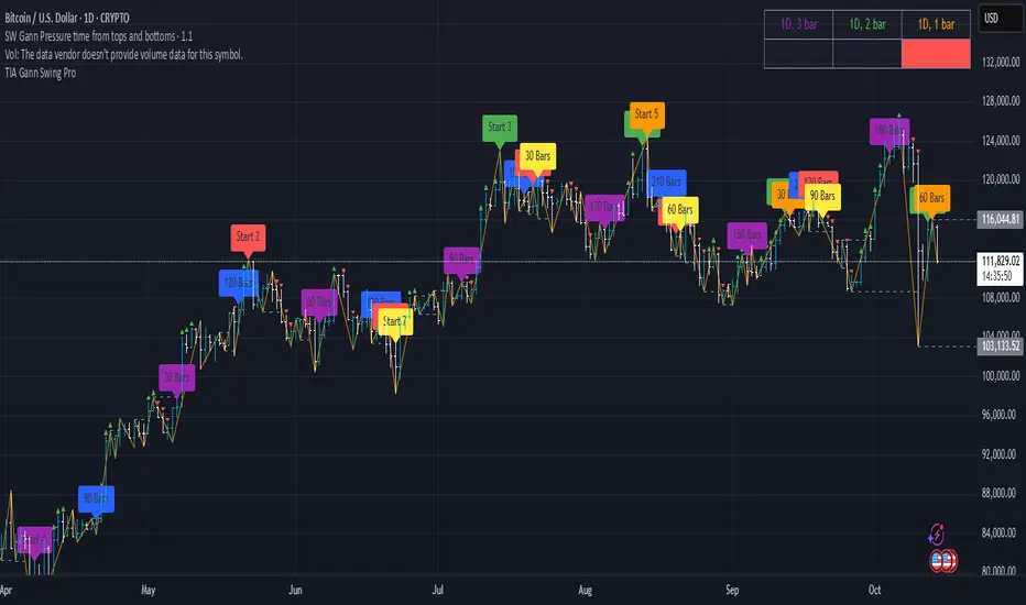
SW Gann Pressure time from tops and bottomsW.D. Gann's trading techniques often emphasized the significance of time in the markets, believing that specific time intervals could influence price movements. Here’s how the 30, 60, 90, 120, 180, and 270 bar intervals relate to Gann's rules:
1. **30 Bars**:
- Gann often viewed shorter time frames as critical for identifying short-term trends. A 30-bar interval can signify minor cycles or potential turning points in price.
2. **60 Bars**:
- This interval is significant as Gann believed in the importance of quarterly cycles. A 60-bar mark could indicate a completion of a two-month cycle, often leading to retracements or reversals.
3. **90 Bars**:
- Gann considered 90 days (or bars) to represent a quarter. This interval can signify a substantial shift in market sentiment or a pivotal point in a longer trend.
4. **120 Bars**:
- The 120-bar mark corresponds to about four months. Gann viewed longer intervals as more significant, often leading to major shifts in market trends.
5. **180 Bars**:
- A 180-bar period relates to a semi-annual cycle, which Gann regarded as critical for major support and resistance levels. Price action around this interval can reveal potential long-term trend reversals.
6. **270 Bars**:
- Gann believed that longer cycles, such as 270 bars (approximately nine months), could indicate significant market phases. This interval may represent major turning points and help identify long-term trends.
### Application in Trading:
- **Identifying Trends**: Traders can use these intervals to spot potential trend reversals or continuations based on Gann’s principles of market cycles.
- **Setting Targets and Stops**: Knowing where these key bars fall can help in setting profit targets and stop-loss orders.
- **Analyzing Market Sentiment**: Price reactions at these intervals can provide insights into market psychology and sentiment shifts.
By marking these intervals on a chart, traders can visually assess when price action aligns with Gann's theories, helping them make more informed trading decisions based on historical patterns and cycles.
Cerca negli script per "欧元汇率走势30天"
30D Vs 90D Historical VolatilityVolatility equals risk for an underlying asset's price meaning bullish volatility is bearish for prices while bearish volatility is bullish. This compares 30-Day Historical Volatility to 90-Day Historical Volatility.
When the 30-Day crosses under the 90-day, this is typically when asset prices enter a bullish trend.
Conversely, When the 30-Day crosses above the 90-Day, this is when asset prices enter a bearish trend.
Peaks in volatility are bullish divergences while troughs are bearish divergences.

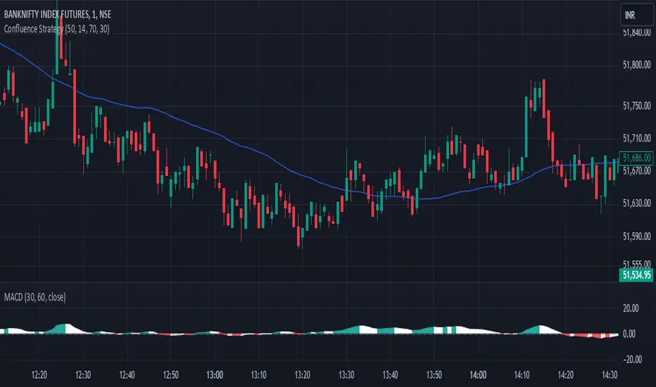
Confluence StrategyOverview of Confluence Strategy
The Confluence Strategy in trading refers to the combination of multiple technical indicators, support/resistance levels, and chart patterns to identify high-probability trading opportunities. The idea is that when several indicators agree on a price movement, the likelihood of that movement being successful increases.
Key Components
Technical Indicators:
Moving Averages (MA): Commonly used to determine the trend direction. Look for crossovers (e.g., the 50-day MA crossing above the 200-day MA).
Relative Strength Index (RSI): Helps identify overbought or oversold conditions. A reading above 70 may indicate overbought conditions, while below 30 suggests oversold.
MACD (Moving Average Convergence Divergence): Useful for spotting changes in momentum. Look for MACD crossovers and divergence from price.
Support and Resistance Levels:
Identify key levels where price has historically reversed. These can be drawn from previous highs/lows, Fibonacci retracement levels, or psychological price levels.
Chart Patterns:
Patterns like head and shoulders, double tops/bottoms, or flags can indicate potential reversals or continuations in price.
Strategy Implementation
Set Up Your Chart:
Add the desired indicators (e.g., MA, RSI, MACD) to your TradingView chart.
Mark significant support and resistance levels.
Identify Confluence Points:
Look for situations where multiple indicators align. For instance, if the price is near a support level, the RSI is below 30, and the MACD shows bullish divergence, this may signal a buying opportunity.
Entry and Exit Points:
Entry: Place a trade when your confluence conditions are met. Use limit orders for better prices.
Exit: Set profit targets based on resistance levels or use trailing stops. Consider the risk-reward ratio to ensure your trades are favorable.
Risk Management:
Always implement stop-loss orders to protect against unexpected market moves. Position size should reflect your risk tolerance.
Example of a Confluence Trade
Setup:
Price approaches a strong support level.
RSI shows oversold conditions (below 30).
The 50-day MA is about to cross above the 200-day MA (bullish crossover).
Action:
Enter a long position as the conditions align.
Set a stop loss just below the support level and a take profit at the next resistance level.
Conclusion
The Confluence Strategy can significantly enhance trading accuracy by ensuring that multiple indicators support a trade decision. Traders on TradingView can customize their indicators and charts to fit their personal trading styles, making it a flexible approach to technical analysis.
Universal Ratio Trend Matrix [InvestorUnknown]The Universal Ratio Trend Matrix is designed for trend analysis on asset/asset ratios, supporting up to 40 different assets. Its primary purpose is to help identify which assets are outperforming others within a selection, providing a broad overview of market trends through a matrix of ratios. The indicator automatically expands the matrix based on the number of assets chosen, simplifying the process of comparing multiple assets in terms of performance.
Key features include the ability to choose from a narrow selection of indicators to perform the ratio trend analysis, allowing users to apply well-defined metrics to their comparison.
Drawback: Due to the computational intensity involved in calculating ratios across many assets, the indicator has a limitation related to loading speed. TradingView has time limits for calculations, and for users on the basic (free) plan, this could result in frequent errors due to exceeded time limits. To use the indicator effectively, users with any paid plans should run it on timeframes higher than 8h (the lowest timeframe on which it managed to load with 40 assets), as lower timeframes may not reliably load.
Indicators:
RSI_raw: Simple function to calculate the Relative Strength Index (RSI) of a source (asset price).
RSI_sma: Calculates RSI followed by a Simple Moving Average (SMA).
RSI_ema: Calculates RSI followed by an Exponential Moving Average (EMA).
CCI: Calculates the Commodity Channel Index (CCI).
Fisher: Implements the Fisher Transform to normalize prices.
Utility Functions:
f_remove_exchange_name: Strips the exchange name from asset tickers (e.g., "INDEX:BTCUSD" to "BTCUSD").
f_remove_exchange_name(simple string name) =>
string parts = str.split(name, ":")
string result = array.size(parts) > 1 ? array.get(parts, 1) : name
result
f_get_price: Retrieves the closing price of a given asset ticker using request.security().
f_constant_src: Checks if the source data is constant by comparing multiple consecutive values.
Inputs:
General settings allow users to select the number of tickers for analysis (used_assets) and choose the trend indicator (RSI, CCI, Fisher, etc.).
Table settings customize how trend scores are displayed in terms of text size, header visibility, highlighting options, and top-performing asset identification.
The script includes inputs for up to 40 assets, allowing the user to select various cryptocurrencies (e.g., BTCUSD, ETHUSD, SOLUSD) or other assets for trend analysis.
Price Arrays:
Price values for each asset are stored in variables (price_a1 to price_a40) initialized as na. These prices are updated only for the number of assets specified by the user (used_assets).
Trend scores for each asset are stored in separate arrays
// declare price variables as "na"
var float price_a1 = na, var float price_a2 = na, var float price_a3 = na, var float price_a4 = na, var float price_a5 = na
var float price_a6 = na, var float price_a7 = na, var float price_a8 = na, var float price_a9 = na, var float price_a10 = na
var float price_a11 = na, var float price_a12 = na, var float price_a13 = na, var float price_a14 = na, var float price_a15 = na
var float price_a16 = na, var float price_a17 = na, var float price_a18 = na, var float price_a19 = na, var float price_a20 = na
var float price_a21 = na, var float price_a22 = na, var float price_a23 = na, var float price_a24 = na, var float price_a25 = na
var float price_a26 = na, var float price_a27 = na, var float price_a28 = na, var float price_a29 = na, var float price_a30 = na
var float price_a31 = na, var float price_a32 = na, var float price_a33 = na, var float price_a34 = na, var float price_a35 = na
var float price_a36 = na, var float price_a37 = na, var float price_a38 = na, var float price_a39 = na, var float price_a40 = na
// create "empty" arrays to store trend scores
var a1_array = array.new_int(40, 0), var a2_array = array.new_int(40, 0), var a3_array = array.new_int(40, 0), var a4_array = array.new_int(40, 0)
var a5_array = array.new_int(40, 0), var a6_array = array.new_int(40, 0), var a7_array = array.new_int(40, 0), var a8_array = array.new_int(40, 0)
var a9_array = array.new_int(40, 0), var a10_array = array.new_int(40, 0), var a11_array = array.new_int(40, 0), var a12_array = array.new_int(40, 0)
var a13_array = array.new_int(40, 0), var a14_array = array.new_int(40, 0), var a15_array = array.new_int(40, 0), var a16_array = array.new_int(40, 0)
var a17_array = array.new_int(40, 0), var a18_array = array.new_int(40, 0), var a19_array = array.new_int(40, 0), var a20_array = array.new_int(40, 0)
var a21_array = array.new_int(40, 0), var a22_array = array.new_int(40, 0), var a23_array = array.new_int(40, 0), var a24_array = array.new_int(40, 0)
var a25_array = array.new_int(40, 0), var a26_array = array.new_int(40, 0), var a27_array = array.new_int(40, 0), var a28_array = array.new_int(40, 0)
var a29_array = array.new_int(40, 0), var a30_array = array.new_int(40, 0), var a31_array = array.new_int(40, 0), var a32_array = array.new_int(40, 0)
var a33_array = array.new_int(40, 0), var a34_array = array.new_int(40, 0), var a35_array = array.new_int(40, 0), var a36_array = array.new_int(40, 0)
var a37_array = array.new_int(40, 0), var a38_array = array.new_int(40, 0), var a39_array = array.new_int(40, 0), var a40_array = array.new_int(40, 0)
f_get_price(simple string ticker) =>
request.security(ticker, "", close)
// Prices for each USED asset
f_get_asset_price(asset_number, ticker) =>
if (used_assets >= asset_number)
f_get_price(ticker)
else
na
// overwrite empty variables with the prices if "used_assets" is greater or equal to the asset number
if barstate.isconfirmed // use barstate.isconfirmed to avoid "na prices" and calculation errors that result in empty cells in the table
price_a1 := f_get_asset_price(1, asset1), price_a2 := f_get_asset_price(2, asset2), price_a3 := f_get_asset_price(3, asset3), price_a4 := f_get_asset_price(4, asset4)
price_a5 := f_get_asset_price(5, asset5), price_a6 := f_get_asset_price(6, asset6), price_a7 := f_get_asset_price(7, asset7), price_a8 := f_get_asset_price(8, asset8)
price_a9 := f_get_asset_price(9, asset9), price_a10 := f_get_asset_price(10, asset10), price_a11 := f_get_asset_price(11, asset11), price_a12 := f_get_asset_price(12, asset12)
price_a13 := f_get_asset_price(13, asset13), price_a14 := f_get_asset_price(14, asset14), price_a15 := f_get_asset_price(15, asset15), price_a16 := f_get_asset_price(16, asset16)
price_a17 := f_get_asset_price(17, asset17), price_a18 := f_get_asset_price(18, asset18), price_a19 := f_get_asset_price(19, asset19), price_a20 := f_get_asset_price(20, asset20)
price_a21 := f_get_asset_price(21, asset21), price_a22 := f_get_asset_price(22, asset22), price_a23 := f_get_asset_price(23, asset23), price_a24 := f_get_asset_price(24, asset24)
price_a25 := f_get_asset_price(25, asset25), price_a26 := f_get_asset_price(26, asset26), price_a27 := f_get_asset_price(27, asset27), price_a28 := f_get_asset_price(28, asset28)
price_a29 := f_get_asset_price(29, asset29), price_a30 := f_get_asset_price(30, asset30), price_a31 := f_get_asset_price(31, asset31), price_a32 := f_get_asset_price(32, asset32)
price_a33 := f_get_asset_price(33, asset33), price_a34 := f_get_asset_price(34, asset34), price_a35 := f_get_asset_price(35, asset35), price_a36 := f_get_asset_price(36, asset36)
price_a37 := f_get_asset_price(37, asset37), price_a38 := f_get_asset_price(38, asset38), price_a39 := f_get_asset_price(39, asset39), price_a40 := f_get_asset_price(40, asset40)
Universal Indicator Calculation (f_calc_score):
This function allows switching between different trend indicators (RSI, CCI, Fisher) for flexibility.
It uses a switch-case structure to calculate the indicator score, where a positive trend is denoted by 1 and a negative trend by 0. Each indicator has its own logic to determine whether the asset is trending up or down.
// use switch to allow "universality" in indicator selection
f_calc_score(source, trend_indicator, int_1, int_2) =>
int score = na
if (not f_constant_src(source)) and source > 0.0 // Skip if you are using the same assets for ratio (for example BTC/BTC)
x = switch trend_indicator
"RSI (Raw)" => RSI_raw(source, int_1)
"RSI (SMA)" => RSI_sma(source, int_1, int_2)
"RSI (EMA)" => RSI_ema(source, int_1, int_2)
"CCI" => CCI(source, int_1)
"Fisher" => Fisher(source, int_1)
y = switch trend_indicator
"RSI (Raw)" => x > 50 ? 1 : 0
"RSI (SMA)" => x > 50 ? 1 : 0
"RSI (EMA)" => x > 50 ? 1 : 0
"CCI" => x > 0 ? 1 : 0
"Fisher" => x > x ? 1 : 0
score := y
else
score := 0
score
Array Setting Function (f_array_set):
This function populates an array with scores calculated for each asset based on a base price (p_base) divided by the prices of the individual assets.
It processes multiple assets (up to 40), calling the f_calc_score function for each.
// function to set values into the arrays
f_array_set(a_array, p_base) =>
array.set(a_array, 0, f_calc_score(p_base / price_a1, trend_indicator, int_1, int_2))
array.set(a_array, 1, f_calc_score(p_base / price_a2, trend_indicator, int_1, int_2))
array.set(a_array, 2, f_calc_score(p_base / price_a3, trend_indicator, int_1, int_2))
array.set(a_array, 3, f_calc_score(p_base / price_a4, trend_indicator, int_1, int_2))
array.set(a_array, 4, f_calc_score(p_base / price_a5, trend_indicator, int_1, int_2))
array.set(a_array, 5, f_calc_score(p_base / price_a6, trend_indicator, int_1, int_2))
array.set(a_array, 6, f_calc_score(p_base / price_a7, trend_indicator, int_1, int_2))
array.set(a_array, 7, f_calc_score(p_base / price_a8, trend_indicator, int_1, int_2))
array.set(a_array, 8, f_calc_score(p_base / price_a9, trend_indicator, int_1, int_2))
array.set(a_array, 9, f_calc_score(p_base / price_a10, trend_indicator, int_1, int_2))
array.set(a_array, 10, f_calc_score(p_base / price_a11, trend_indicator, int_1, int_2))
array.set(a_array, 11, f_calc_score(p_base / price_a12, trend_indicator, int_1, int_2))
array.set(a_array, 12, f_calc_score(p_base / price_a13, trend_indicator, int_1, int_2))
array.set(a_array, 13, f_calc_score(p_base / price_a14, trend_indicator, int_1, int_2))
array.set(a_array, 14, f_calc_score(p_base / price_a15, trend_indicator, int_1, int_2))
array.set(a_array, 15, f_calc_score(p_base / price_a16, trend_indicator, int_1, int_2))
array.set(a_array, 16, f_calc_score(p_base / price_a17, trend_indicator, int_1, int_2))
array.set(a_array, 17, f_calc_score(p_base / price_a18, trend_indicator, int_1, int_2))
array.set(a_array, 18, f_calc_score(p_base / price_a19, trend_indicator, int_1, int_2))
array.set(a_array, 19, f_calc_score(p_base / price_a20, trend_indicator, int_1, int_2))
array.set(a_array, 20, f_calc_score(p_base / price_a21, trend_indicator, int_1, int_2))
array.set(a_array, 21, f_calc_score(p_base / price_a22, trend_indicator, int_1, int_2))
array.set(a_array, 22, f_calc_score(p_base / price_a23, trend_indicator, int_1, int_2))
array.set(a_array, 23, f_calc_score(p_base / price_a24, trend_indicator, int_1, int_2))
array.set(a_array, 24, f_calc_score(p_base / price_a25, trend_indicator, int_1, int_2))
array.set(a_array, 25, f_calc_score(p_base / price_a26, trend_indicator, int_1, int_2))
array.set(a_array, 26, f_calc_score(p_base / price_a27, trend_indicator, int_1, int_2))
array.set(a_array, 27, f_calc_score(p_base / price_a28, trend_indicator, int_1, int_2))
array.set(a_array, 28, f_calc_score(p_base / price_a29, trend_indicator, int_1, int_2))
array.set(a_array, 29, f_calc_score(p_base / price_a30, trend_indicator, int_1, int_2))
array.set(a_array, 30, f_calc_score(p_base / price_a31, trend_indicator, int_1, int_2))
array.set(a_array, 31, f_calc_score(p_base / price_a32, trend_indicator, int_1, int_2))
array.set(a_array, 32, f_calc_score(p_base / price_a33, trend_indicator, int_1, int_2))
array.set(a_array, 33, f_calc_score(p_base / price_a34, trend_indicator, int_1, int_2))
array.set(a_array, 34, f_calc_score(p_base / price_a35, trend_indicator, int_1, int_2))
array.set(a_array, 35, f_calc_score(p_base / price_a36, trend_indicator, int_1, int_2))
array.set(a_array, 36, f_calc_score(p_base / price_a37, trend_indicator, int_1, int_2))
array.set(a_array, 37, f_calc_score(p_base / price_a38, trend_indicator, int_1, int_2))
array.set(a_array, 38, f_calc_score(p_base / price_a39, trend_indicator, int_1, int_2))
array.set(a_array, 39, f_calc_score(p_base / price_a40, trend_indicator, int_1, int_2))
a_array
Conditional Array Setting (f_arrayset):
This function checks if the number of used assets is greater than or equal to a specified number before populating the arrays.
// only set values into arrays for USED assets
f_arrayset(asset_number, a_array, p_base) =>
if (used_assets >= asset_number)
f_array_set(a_array, p_base)
else
na
Main Logic
The main logic initializes arrays to store scores for each asset. Each array corresponds to one asset's performance score.
Setting Trend Values: The code calls f_arrayset for each asset, populating the respective arrays with calculated scores based on the asset prices.
Combining Arrays: A combined_array is created to hold all the scores from individual asset arrays. This array facilitates further analysis, allowing for an overview of the performance scores of all assets at once.
// create a combined array (work-around since pinescript doesn't support having array of arrays)
var combined_array = array.new_int(40 * 40, 0)
if barstate.islast
for i = 0 to 39
array.set(combined_array, i, array.get(a1_array, i))
array.set(combined_array, i + (40 * 1), array.get(a2_array, i))
array.set(combined_array, i + (40 * 2), array.get(a3_array, i))
array.set(combined_array, i + (40 * 3), array.get(a4_array, i))
array.set(combined_array, i + (40 * 4), array.get(a5_array, i))
array.set(combined_array, i + (40 * 5), array.get(a6_array, i))
array.set(combined_array, i + (40 * 6), array.get(a7_array, i))
array.set(combined_array, i + (40 * 7), array.get(a8_array, i))
array.set(combined_array, i + (40 * 8), array.get(a9_array, i))
array.set(combined_array, i + (40 * 9), array.get(a10_array, i))
array.set(combined_array, i + (40 * 10), array.get(a11_array, i))
array.set(combined_array, i + (40 * 11), array.get(a12_array, i))
array.set(combined_array, i + (40 * 12), array.get(a13_array, i))
array.set(combined_array, i + (40 * 13), array.get(a14_array, i))
array.set(combined_array, i + (40 * 14), array.get(a15_array, i))
array.set(combined_array, i + (40 * 15), array.get(a16_array, i))
array.set(combined_array, i + (40 * 16), array.get(a17_array, i))
array.set(combined_array, i + (40 * 17), array.get(a18_array, i))
array.set(combined_array, i + (40 * 18), array.get(a19_array, i))
array.set(combined_array, i + (40 * 19), array.get(a20_array, i))
array.set(combined_array, i + (40 * 20), array.get(a21_array, i))
array.set(combined_array, i + (40 * 21), array.get(a22_array, i))
array.set(combined_array, i + (40 * 22), array.get(a23_array, i))
array.set(combined_array, i + (40 * 23), array.get(a24_array, i))
array.set(combined_array, i + (40 * 24), array.get(a25_array, i))
array.set(combined_array, i + (40 * 25), array.get(a26_array, i))
array.set(combined_array, i + (40 * 26), array.get(a27_array, i))
array.set(combined_array, i + (40 * 27), array.get(a28_array, i))
array.set(combined_array, i + (40 * 28), array.get(a29_array, i))
array.set(combined_array, i + (40 * 29), array.get(a30_array, i))
array.set(combined_array, i + (40 * 30), array.get(a31_array, i))
array.set(combined_array, i + (40 * 31), array.get(a32_array, i))
array.set(combined_array, i + (40 * 32), array.get(a33_array, i))
array.set(combined_array, i + (40 * 33), array.get(a34_array, i))
array.set(combined_array, i + (40 * 34), array.get(a35_array, i))
array.set(combined_array, i + (40 * 35), array.get(a36_array, i))
array.set(combined_array, i + (40 * 36), array.get(a37_array, i))
array.set(combined_array, i + (40 * 37), array.get(a38_array, i))
array.set(combined_array, i + (40 * 38), array.get(a39_array, i))
array.set(combined_array, i + (40 * 39), array.get(a40_array, i))
Calculating Sums: A separate array_sums is created to store the total score for each asset by summing the values of their respective score arrays. This allows for easy comparison of overall performance.
Ranking Assets: The final part of the code ranks the assets based on their total scores stored in array_sums. It assigns a rank to each asset, where the asset with the highest score receives the highest rank.
// create array for asset RANK based on array.sum
var ranks = array.new_int(used_assets, 0)
// for loop that calculates the rank of each asset
if barstate.islast
for i = 0 to (used_assets - 1)
int rank = 1
for x = 0 to (used_assets - 1)
if i != x
if array.get(array_sums, i) < array.get(array_sums, x)
rank := rank + 1
array.set(ranks, i, rank)
Dynamic Table Creation
Initialization: The table is initialized with a base structure that includes headers for asset names, scores, and ranks. The headers are set to remain constant, ensuring clarity for users as they interpret the displayed data.
Data Population: As scores are calculated for each asset, the corresponding values are dynamically inserted into the table. This is achieved through a loop that iterates over the scores and ranks stored in the combined_array and array_sums, respectively.
Automatic Extending Mechanism
Variable Asset Count: The code checks the number of assets defined by the user. Instead of hardcoding the number of rows in the table, it uses a variable to determine the extent of the data that needs to be displayed. This allows the table to expand or contract based on the number of assets being analyzed.
Dynamic Row Generation: Within the loop that populates the table, the code appends new rows for each asset based on the current asset count. The structure of each row includes the asset name, its score, and its rank, ensuring that the table remains consistent regardless of how many assets are involved.
// Automatically extending table based on the number of used assets
var table table = table.new(position.bottom_center, 50, 50, color.new(color.black, 100), color.white, 3, color.white, 1)
if barstate.islast
if not hide_head
table.cell(table, 0, 0, "Universal Ratio Trend Matrix", text_color = color.white, bgcolor = #010c3b, text_size = fontSize)
table.merge_cells(table, 0, 0, used_assets + 3, 0)
if not hide_inps
table.cell(table, 0, 1,
text = "Inputs: You are using " + str.tostring(trend_indicator) + ", which takes: " + str.tostring(f_get_input(trend_indicator)),
text_color = color.white, text_size = fontSize), table.merge_cells(table, 0, 1, used_assets + 3, 1)
table.cell(table, 0, 2, "Assets", text_color = color.white, text_size = fontSize, bgcolor = #010c3b)
for x = 0 to (used_assets - 1)
table.cell(table, x + 1, 2, text = str.tostring(array.get(assets, x)), text_color = color.white, bgcolor = #010c3b, text_size = fontSize)
table.cell(table, 0, x + 3, text = str.tostring(array.get(assets, x)), text_color = color.white, bgcolor = f_asset_col(array.get(ranks, x)), text_size = fontSize)
for r = 0 to (used_assets - 1)
for c = 0 to (used_assets - 1)
table.cell(table, c + 1, r + 3, text = str.tostring(array.get(combined_array, c + (r * 40))),
text_color = hl_type == "Text" ? f_get_col(array.get(combined_array, c + (r * 40))) : color.white, text_size = fontSize,
bgcolor = hl_type == "Background" ? f_get_col(array.get(combined_array, c + (r * 40))) : na)
for x = 0 to (used_assets - 1)
table.cell(table, x + 1, x + 3, "", bgcolor = #010c3b)
table.cell(table, used_assets + 1, 2, "", bgcolor = #010c3b)
for x = 0 to (used_assets - 1)
table.cell(table, used_assets + 1, x + 3, "==>", text_color = color.white)
table.cell(table, used_assets + 2, 2, "SUM", text_color = color.white, text_size = fontSize, bgcolor = #010c3b)
table.cell(table, used_assets + 3, 2, "RANK", text_color = color.white, text_size = fontSize, bgcolor = #010c3b)
for x = 0 to (used_assets - 1)
table.cell(table, used_assets + 2, x + 3,
text = str.tostring(array.get(array_sums, x)),
text_color = color.white, text_size = fontSize,
bgcolor = f_highlight_sum(array.get(array_sums, x), array.get(ranks, x)))
table.cell(table, used_assets + 3, x + 3,
text = str.tostring(array.get(ranks, x)),
text_color = color.white, text_size = fontSize,
bgcolor = f_highlight_rank(array.get(ranks, x)))

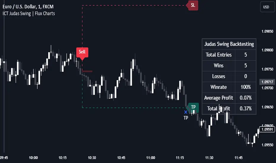
ICT Judas Swing | Flux Charts💎 GENERAL OVERVIEW
Introducing our new ICT Judas Swing Indicator! This indicator is built around the ICT's "Judas Swing" strategy. The strategy looks for a liquidity grab around NY 9:30 session and a Fair Value Gap for entry confirmation. For more information about the process, check the "HOW DOES IT WORK" section.
Features of the new ICT Judas Swing :
Implementation of ICT's Judas Swing Strategy
2 Different TP / SL Methods
Customizable Execution Settings
Customizable Backtesting Dashboard
Alerts for Buy, Sell, TP & SL Signals
📌 HOW DOES IT WORK ?
The strategy begins by identifying the New York session from 9:30 to 9:45 and marking recent liquidity zones. These liquidity zones are determined by locating high and low pivot points: buyside liquidity zones are identified using high pivots that haven't been invalidated, while sellside liquidity zones are found using low pivots. A break of either buyside or sellside liquidity must occur during the 9:30-9:45 session, which is interpreted as a liquidity grab by smart money. The strategy assumes that after this liquidity grab, the price will reverse and move in the opposite direction. For entry confirmation, a fair value gap (FVG) in the opposite direction of the liquidity grab is required. A buyside liquidity grab calls for a bearish FVG, while a sellside grab requires a bullish FVG. Based on the type of FVG—bullish for buys and bearish for sells—the indicator will then generate a Buy or Sell signal.
After the Buy or Sell signal, the indicator immediately draws the take-profit (TP) and stop-loss (SL) targets. The indicator has three different TP & SL modes, explained in the "Settings" section of this write-up.
You can set up alerts for entry and TP & SL signals, and also check the current performance of the indicator and adjust the settings accordingly to the current ticker using the backtesting dashboard.
🚩 UNIQUENESS
This indicator is an all-in-one suit for the ICT's Judas Swing concept. It's capable of plotting the strategy, giving signals, a backtesting dashboard and alerts feature. Different and customizable algorithm modes will help the trader fine-tune the indicator for the asset they are currently trading. Three different TP / SL modes are available to suit your needs. The backtesting dashboard allows you to see how your settings perform in the current ticker. You can also set up alerts to get informed when the strategy is executable for different tickers.
⚙️ SETTINGS
1. General Configuration
Swing Length -> The swing length for pivot detection. Higher settings will result in
FVG Detection Sensitivity -> You may select between Low, Normal, High or Extreme FVG detection sensitivity. This will essentially determine the size of the spotted FVGs, with lower sensitivies resulting in spotting bigger FVGs, and higher sensitivies resulting in spotting all sizes of FVGs.
2. TP / SL
TP / SL Method ->
a) Dynamic: The TP / SL zones will be auto-determined by the algorithm based on the Average True Range (ATR) of the current ticker.
b) Fixed : You can adjust the exact TP / SL ratios from the settings below.
Dynamic Risk -> The risk you're willing to take if "Dynamic" TP / SL Method is selected. Higher risk usually means a better winrate at the cost of losing more if the strategy fails. This setting is has a crucial effect on the performance of the indicator, as different tickers may have different volatility so the indicator may have increased performance when this setting is correctly adjusted.
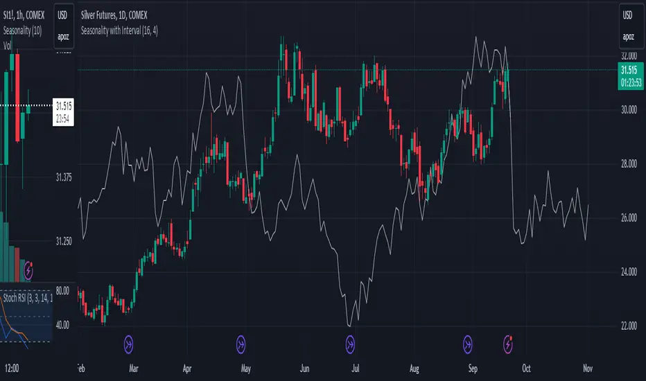
Seasonality with Custom IntervalSeasonality with Custom Interval Lookback
by TradersPod
Description:
This script is a modified version of Kaschko's original Seasonal Trend with Interval Lookback indicator, designed to help traders analyze seasonal trends over customizable intervals. The modifications in this version provide enhanced flexibility and improved visualization, making it a valuable tool for analyzing seasonal patterns in various markets.
Key Features:
1. Custom Lookback Multiplier: The script allows users to adjust the lookback period with a multiplier, giving more control over the number of years analyzed for seasonality. This feature is especially useful for traders looking to tailor the analysis based on different market cycles or election cycles.
2. Enhanced Visualization: Users can customize the color and line width of the plotted seasonality line for better readability. The smoothing parameter has been added to allow for flexible moving averages, reducing noise in the trend visualization.
3 Detailed Chart Plotting: The script plots the trading week of the year (TWOY), trading day of the month (TDOM), and trading day of the year (TDOY) on the status line, providing users with additional insights into how seasonal trends affect price movements.
How to Use:
1. Lookback Period: Set the number of years to look back. For example, if you set it to 16 years, the script will gather data from the last 16 years.
2. Interval Years: You can set an interval (e.g., 4 years for U.S. elections) to focus on specific years:
Interval = 0: This setting will use all years within the lookback period.
Interval > 0: This setting will use only every nth year, based on the interval you set (e.g., 4 for U.S. elections, 10 for decennial years).
3 Future Projections: You can specify how many bars into the future the script should project the seasonal trend.
Example Settings:
>Lookback Period: 16 years.
>Interval: 4 years (this would focus on U.S. election years).
>]Future Projections: 30 bars (the seasonal trend is projected 30 bars into the future).
Intended Use : This indicator is ideal for traders who:
>Want to analyze how market prices react to seasonal cycles.
>Need flexible, customizable tools for tracking longer-term trends.
>Prefer visual clarity in their seasonal trend analysis with adjustable settings for better readability.
How It Works:
>The script calculates the average price change for each trading day, week, or month, using a lookback period of up to 30 years. It then smooths the seasonal trend using a customizable moving average and projects the trend into the future, allowing users to forecast potential price movements based on historical seasonal patterns.
>The script also offers a projection of future seasonality by plotting the seasonal trend up to 252 bars into the future, with options to offset the start of the seasonality.
Notes:
>This script is open-source under the Mozilla Public License 2.0.
>Original script by Kaschko. Modifications by TradersPod.
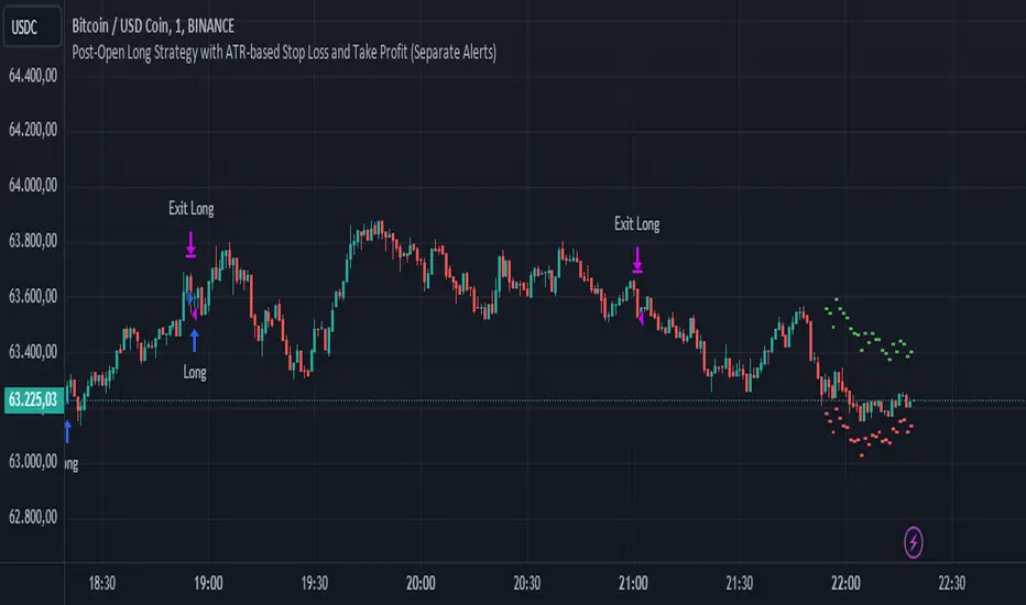
Post-Open Long Strategy with ATR-based Stop Loss and Take ProfitThe "Post-Open Long Strategy with ATR-Based Stop Loss and Take Profit" is designed to identify buying opportunities after the German and US markets open. It combines various technical indicators to filter entry signals, focusing on breakout moments following price lateralization periods.
Key Components and Their Interaction:
Bollinger Bands (BB):
Description: Uses BB with a 14-period length and standard deviation multiplier of 1.5, creating narrower bands for lower timeframes.
Role in the Strategy: Identifies low volatility phases (lateralization). The lateralization condition is met when the price is near the simple moving average of the BB, suggesting an imminent increase in volatility.
Exponential Moving Averages (EMA):
10-period EMA: Quickly detects short-term trend direction.
200-period EMA: Filters long-term trends, ensuring entries occur in a bullish market.
Interaction: Positions are entered only if the price is above both EMAs, indicating a consolidated positive trend.
Relative Strength Index (RSI):
Description: 7-period RSI with a threshold above 30.
Role in the Strategy: Confirms the market is not oversold, supporting the validity of the buy signal.
Average Directional Index (ADX):
Description: 7-period ADX with 7-period smoothing and a threshold above 10.
Role in the Strategy: Assesses trend strength. An ADX above 10 indicates sufficient momentum to justify entry.
Average True Range (ATR) for Dynamic Stop Loss and Take Profit:
Description: 14-period ATR with multipliers of 2.0 for Stop Loss and 4.0 for Take Profit.
Role in the Strategy: Adjusts exit levels based on current volatility, enhancing risk management.
Resistance Identification and Breakout:
Description: Analyzes the highs of the last 20 candles to identify resistance levels with at least two touches.
Role in the Strategy: A breakout above this level signals a potential continuation of the bullish trend.
Time Filters and Market Conditions:
Trading Hours: Operates only during the opening of the German market (8:00 - 12:00) and US market (15:30 - 19:00).
Panic Candle: The current candle must close negative, leveraging potential emotional reactions in the market.
Avoiding Entry During Pullbacks:
Description: Checks that the two previous candles are not both bearish.
Role in the Strategy: Avoids entering during a potential pullback, improving trade success probability.
Post-Open Long Strategy with ATR-Based Stop Loss and Take Profit
The "Post-Open Long Strategy with ATR-Based Stop Loss and Take Profit" is designed to identify buying opportunities after the German and US markets open. It combines various technical indicators to filter entry signals, focusing on breakout moments following price lateralization periods.
Key Components and Their Interaction:
Bollinger Bands (BB):
Description: Uses BB with a 14-period length and standard deviation multiplier of 1.5, creating narrower bands for lower timeframes.
Role in the Strategy: Identifies low volatility phases (lateralization). The lateralization condition is met when the price is near the simple moving average of the BB, suggesting an imminent increase in volatility.
Exponential Moving Averages (EMA):
10-period EMA: Quickly detects short-term trend direction.
200-period EMA: Filters long-term trends, ensuring entries occur in a bullish market.
Interaction: Positions are entered only if the price is above both EMAs, indicating a consolidated positive trend.
Relative Strength Index (RSI):
Description: 7-period RSI with a threshold above 30.
Role in the Strategy: Confirms the market is not oversold, supporting the validity of the buy signal.
Average Directional Index (ADX):
Description: 7-period ADX with 7-period smoothing and a threshold above 10.
Role in the Strategy: Assesses trend strength. An ADX above 10 indicates sufficient momentum to justify entry.
Average True Range (ATR) for Dynamic Stop Loss and Take Profit:
Description: 14-period ATR with multipliers of 2.0 for Stop Loss and 4.0 for Take Profit.
Role in the Strategy: Adjusts exit levels based on current volatility, enhancing risk management.
Resistance Identification and Breakout:
Description: Analyzes the highs of the last 20 candles to identify resistance levels with at least two touches.
Role in the Strategy: A breakout above this level signals a potential continuation of the bullish trend.
Time Filters and Market Conditions:
Trading Hours: Operates only during the opening of the German market (8:00 - 12:00) and US market (15:30 - 19:00).
Panic Candle: The current candle must close negative, leveraging potential emotional reactions in the market.
Avoiding Entry During Pullbacks:
Description: Checks that the two previous candles are not both bearish.
Role in the Strategy: Avoids entering during a potential pullback, improving trade success probability.
Entry and Exit Conditions:
Long Entry:
The price breaks above the identified resistance.
The market is in a lateralization phase with low volatility.
The price is above the 10 and 200-period EMAs.
RSI is above 30, and ADX is above 10.
No short-term downtrend is detected.
The last two candles are not both bearish.
The current candle is a "panic candle" (negative close).
Order Execution: The order is executed at the close of the candle that meets all conditions.
Exit from Position:
Dynamic Stop Loss: Set at 2 times the ATR below the entry price.
Dynamic Take Profit: Set at 4 times the ATR above the entry price.
The position is automatically closed upon reaching the Stop Loss or Take Profit.
How to Use the Strategy:
Application on Volatile Instruments:
Ideal for financial instruments that show significant volatility during the target market opening hours, such as indices or major forex pairs.
Recommended Timeframes:
Intraday timeframes, such as 5 or 15 minutes, to capture significant post-open moves.
Parameter Customization:
The default parameters are optimized but can be adjusted based on individual preferences and the instrument analyzed.
Backtesting and Optimization:
Backtesting is recommended to evaluate performance and make adjustments if necessary.
Risk Management:
Ensure position sizing respects risk management rules, avoiding risking more than 1-2% of capital per trade.
Originality and Benefits of the Strategy:
Unique Combination of Indicators: Integrates various technical metrics to filter signals, reducing false positives.
Volatility Adaptability: The use of ATR for Stop Loss and Take Profit allows the strategy to adapt to real-time market conditions.
Focus on Post-Lateralization Breakout: Aims to capitalize on significant moves following consolidation periods, often associated with strong directional trends.
Important Notes:
Commissions and Slippage: Include commissions and slippage in settings for more realistic simulations.
Capital Size: Use a realistic trading capital for the average user.
Number of Trades: Ensure backtesting covers a sufficient number of trades to validate the strategy (ideally more than 100 trades).
Warning: Past results do not guarantee future performance. The strategy should be used as part of a comprehensive trading approach.
With this strategy, traders can identify and exploit specific market opportunities supported by a robust set of technical indicators and filters, potentially enhancing their trading decisions during key times of the day.
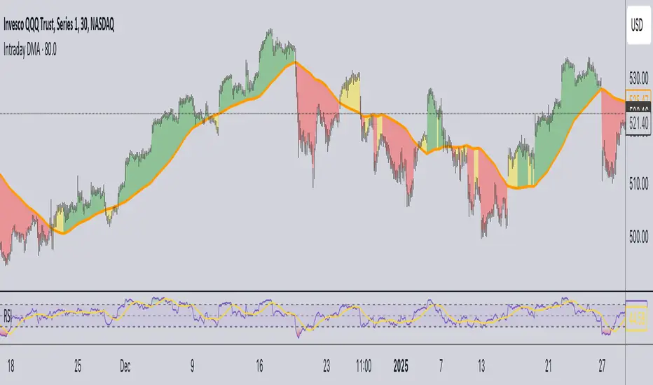
Daily Moving Average for Intraday TimeframesThis indicator provides a dynamic tool for visualizing the Daily Moving Average (DMA) on intraday timeframes.
It allows you to analyze how the price behaves in relation to the daily moving average in timeframes from 1 minute up to 1 day.
KEY FEATURES
DMA on Intraday timeframes only : This indicator is designed to work exclusively on intraday charts with timeframes between 1 minute and 1 day. It will not function on tick, second-based, or daily-and-above charts.
Color-Coded Zones for Trend Identification :
Green Zone: The price is above a rising DMA, signaling a bullish momentum.
Red Zone: The price is below a falling DMA, signaling a bearish momentum.
Yellow Zone: Signaling uncertainty or mixed conditions, where either the price is above a falling DMA or below a rising/flat DMA.
Configurable DMA Period : You can adjust the number of days over which the DMA is calculated (default is 5 days). This can be customized based on your trading strategy or market preferences.
24/7 Market Option : For assets that trade continuously (e.g., cryptocurrencies), activate the "Is trading 24/7?" setting to ensure accurate calculations.
WHAT IS THE DMA AND WHY USE IT INTRADAY?
The Daily Moving Average is a Simple Moving Average indicator used to smooth out price fluctuations over a specified period (in days) and reveal the underlying trend.
Typically, a SMA takes price value for the current timeframe and reveal the trend for this timeframe. It gives you the average price for the last N candles for the given timeframe.
But what makes the Intraday DMA interesting is that it shows the underlying trend of the Daily timeframe on a chart set on a shorter timeframe . This helps to align intraday trades with broader market movements.
HOW IS THE DMA CALCULATED?
If we are to build a N-day Daily Moving Average using a Simple Moving Average, we need to take the amount of candles A needed in that timeframe to account for a period of a day and multiply it by the number of days N of the desired DMA.
So for instance, let say we want to compute the 5-Day DMA on the 10 minute timeframe :
In the 10 minute timeframe there are 39 candles in a day in the regular session.
We would take the 39 candles per day and then multiply that by 5 days. 39 x 5 = 195.
So a 5-day moving average is represented by a simple moving average with a period of 195 when looking at a 10 minute timeframe.
So for each period, to create a 5-day DMA, you would have to set the period of your simple moving average like so :
- 195 minutes = 10 period
- 130 minutes = 15 period
- 65 minutes = 30 period
- 30 minutes = 65 period
- 15 minutes = 130 period
- 10 minutes = 195 period
- 5 minutes = 390 period
and so on.
This indicator attempts to do this calculation for you on any intraday timeframe and whatever the period you want to use is for your DMA. You can create a 10-day moving average, a 30-day moving average, etc.
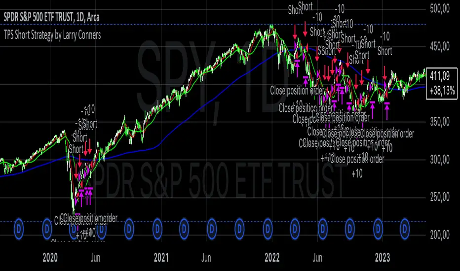
TPS Short Strategy by Larry ConnersThe TPS Short strategy aims to capitalize on extreme overbought conditions in an ETF by employing a scaling-in approach when certain technical indicators signal potential reversals. The strategy is designed to short the ETF when it is deemed overextended, based on the Relative Strength Index (RSI) and moving averages.
Components:
200-Day Simple Moving Average (SMA):
Purpose: Acts as a long-term trend filter. The ETF must be below its 200-day SMA to be eligible for shorting.
Rationale: The 200-day SMA is widely used to gauge the long-term trend of a security. When the price is below this moving average, it is often considered to be in a downtrend (Tushar S. Chande & Stanley Kroll, "The New Technical Trader: Boost Your Profit by Plugging Into the Latest Indicators").
2-Period RSI:
Purpose: Measures the speed and change of price movements to identify overbought conditions.
Criteria: Short 10% of the position when the 2-period RSI is above 75 for two consecutive days.
Rationale: A high RSI value (above 75) indicates that the ETF may be overbought, which could precede a price reversal (J. Welles Wilder, "New Concepts in Technical Trading Systems").
Scaling-In Mechanism:
Purpose: Gradually increase the short position as the ETF price rises beyond previous entry points.
Scaling Strategy:
20% more when the price is higher than the first entry.
30% more when the price is higher than the second entry.
40% more when the price is higher than the third entry.
Rationale: This incremental approach allows for an increased position size in a worsening trend, potentially increasing profitability if the trend continues to align with the strategy’s premise (Marty Schwartz, "Pit Bull: Lessons from Wall Street's Champion Day Trader").
Exit Conditions:
Criteria: Close all positions when the 2-period RSI drops below 30 or the 10-day SMA crosses above the 30-day SMA.
Rationale: A low RSI value (below 30) suggests that the ETF may be oversold and could be poised for a rebound, while the SMA crossover indicates a potential change in the trend (Martin J. Pring, "Technical Analysis Explained").
Risks and Considerations:
Market Risk:
The strategy assumes that the ETF will continue to decline once shorted. However, markets can be unpredictable, and price movements might not align with the strategy's expectations, especially in a volatile market (Nassim Nicholas Taleb, "The Black Swan: The Impact of the Highly Improbable").
Scaling Risks:
Scaling into a position as the price increases may increase exposure to adverse price movements. This method can amplify losses if the market moves against the position significantly before any reversal occurs.
Liquidity Risk:
Depending on the ETF’s liquidity, executing large trades in increments might affect the price and increase trading costs. It is crucial to ensure that the ETF has sufficient liquidity to handle large trades without significant slippage (James Altucher, "Trade Like a Hedge Fund").
Execution Risk:
The strategy relies on timely execution of trades based on specific conditions. Delays or errors in order execution can impact performance, especially in fast-moving markets.
Technical Indicator Limitations:
Technical indicators like RSI and SMA are based on historical data and may not always predict future price movements accurately. They can sometimes produce false signals, leading to potential losses if used in isolation (John Murphy, "Technical Analysis of the Financial Markets").
Conclusion
The TPS Short strategy utilizes a combination of long-term trend filtering, overbought conditions, and incremental shorting to potentially profit from price reversals. While the strategy has a structured approach and leverages well-known technical indicators, it is essential to be aware of the inherent risks, including market volatility, liquidity issues, and potential limitations of technical indicators. As with any trading strategy, thorough backtesting and risk management are crucial to its successful implementation.
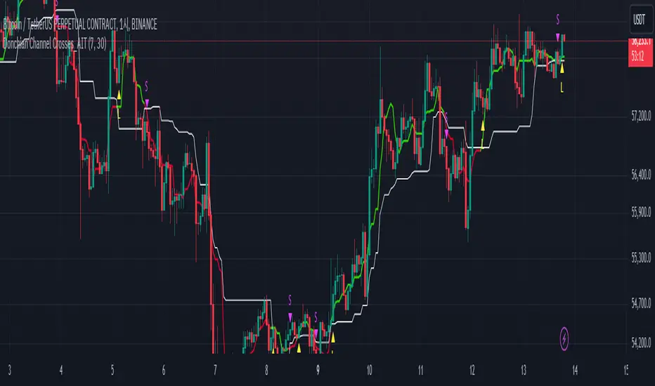
Donchian Channel Crosses_AITIndicator Name: Donchian Channel Crosses_AIT
Programming Language: Pine Script (TradingView)
Description
The Donchian Channel Crosses_AIT indicator is designed to provide trading signals based on the crossover of two Donchian Channels with different lookback periods. The indicator uses two channels, Donchian Channel A (default 7-day period) and Donchian Channel B (default 30-day period), to detect upward or downward momentum shifts. The signals are generated when the middle line of Donchian Channel A crosses above or below the middle line of Donchian Channel B.
Components
Donchian Channel A:
Default period: 7 days (modifiable by the user).
Middle Line: Calculated as the average of the highest high and lowest low over the period.
The middle line changes color depending on its position relative to Donchian Channel B.
Green: When Donchian Channel A's middle line is above Donchian Channel B's middle line.
Red: When Donchian Channel A's middle line is below Donchian Channel B's middle line.
Donchian Channel B:
Default period: 30 days (modifiable by the user).
Middle Line: Also calculated as the average of the highest high and lowest low over the period.
Always displayed as a white line with a line thickness of 1.
Long Signal:
Triggered when the middle line of Donchian Channel A crosses above the middle line of Donchian Channel B.
Displayed as a yellow triangle pointing up (L) below the price bar.
Short Signal:
Triggered when the middle line of Donchian Channel A crosses below the middle line of Donchian Channel B.
Displayed as a fuchsia triangle pointing down (S) above the price bar.
Settings
Donchian Channel A:
Default period: 7 days (modifiable via user input).
Middle line changes color based on its relationship to Donchian Channel B.
Donchian Channel B:
Default period: 30 days (modifiable via user input).
Middle line is always white and displayed with a line thickness of 1.
Signal Display:
Long Signal: A yellow "L" triangle is displayed when Donchian Channel A’s middle line crosses above Donchian Channel B’s middle line.
Short Signal: A fuchsia "S" triangle is displayed when Donchian Channel A’s middle line crosses below Donchian Channel B’s middle line.
Signals can be toggled on or off using the "Show Signals" setting.
Usage
Trend Confirmation:
Use this indicator to confirm trend direction by monitoring the relationship between Donchian Channel A and Donchian Channel B.
Uptrend: When Donchian Channel A’s middle line is above Donchian Channel B’s middle line (green line for Donchian A).
Downtrend: When Donchian Channel A’s middle line is below Donchian Channel B’s middle line (red line for Donchian A).
Entry and Exit Signals:
Long Signal: Enter a buy position when Donchian Channel A crosses above Donchian Channel B.
Short Signal: Enter a sell position when Donchian Channel A crosses below Donchian Channel B.
Visual Representation:
The Donchian Channels are drawn on the price chart, with Donchian Channel A dynamically changing color depending on its relative position to Donchian Channel B.
US Market Support & ResistanceUS Market Support & Resistance Indicator (For 5-30 Minute Timeframes)
This indicator plots key support and resistance levels for the US market based on the high and low of the first candle at the market open. It also shades the area between these levels with a color that dynamically changes to indicate the current trend:
* Green: Price is above the resistance level, suggesting a potential uptrend.
* Red: Price is below the support level, suggesting a potential downtrend.
* Gray: Price is trading between the support and resistance levels, suggesting a sideways trend.
Additionally, the indicator displays a small dashboard in the top right corner of the chart showing the current trend ("Upward", "Downward", or "Sideways") in the corresponding color.
Key Features:
* US Market Time Identification: Accurately identifies US market open and close times in UTC and colors candles red during these times.
* Support & Resistance Plotting: Plots support and resistance lines at the high and low of the first candle at the market open and extends them infinitely on the chart.
* Shaded Area Between Levels: Shades the area between the support and resistance lines with a color that dynamically changes based on the current price location relative to these levels.
* Trend Display: Displays a dashboard showing the current trend based on the shaded area's color.
* Open Alert: Issues an alert when the US market opens.
* Supported Timeframes: Works on timeframes less than 30 minutes and greater than 5 minutes.
* Economic News: Not recommended for use during periods of sporadic economic news releases, as sudden price fluctuations may cause false signals.
How to Use:
* Add the indicator to your chart, ensuring the timeframe is between 5 and 30 minutes.
* Wait for the US market to open.
* Observe the shaded area's color and the dashboard to identify the current trend.
* Use the support and resistance levels to make trading decisions, keeping in mind not to rely solely on it during news releases.
Caution: This indicator relies on support and resistance levels drawn at the US market open and may not always be accurate, especially during periods of high volatility. It should be used in conjunction with other technical analysis tools to confirm the trend and make informed trading decisions.
Note: This description is designed to be compliant with TradingView's policies on indicator publishing.

Key Times & Opening Prices [Olitrades]This indicator plots key time's (opening prices) with the possibility of vertical separators. It was initially created to utilize on the indices futures market, utilizing ICT logic.
These opening prices are often utilized to determine if price is currently at a premium or a discounted value.
The default times include:
Daily Open (18:00 PM)
Midnight (00:00 AM)
Settlement (15:00 PM)
7:30 AM
8:30 AM
9:30 AM (Equities Open)
10:00 AM (Morning 4h Candle Open)
14:00 PM (Afternoon 4h Candle Open)
Along with up to three custom time slots.
All times used in the indicator are Eastern Standard time (New York local time) and will automatically adjust no matter your time zone.
Historical
When in historical mode, the indicator will keep the previous levels so you can easily visualize them and their relation to price.
You can also choose how many past levels you want to see. This allows you to back test only specific days/weeks.
Other Inputs
The indicator contains an adjustable offset, to modify how far the line extends depending on the current timeframe.
Each one of the above-mentioned levels can be turned on and off, including the custom times. You can also choose between plotting just the opening price, a vertical line separator, or both! All of these lines have adjustable styles (dotted, dashed or solid) and width.
They also have custom cut offs. You may choose specific cut off times for custom time slots (when to stop extending the lines), as well as for AM (before noon) default levels and PM (after noon) default levels.
The indicator also allows to show text labels next to these lines, which is set by default but can be turned off. Custom times also include custom text options.

Muti TimeFrame 1st Minute High and a LowThis Pine Script code is designed to plot the high, close, and low prices at exactly 9:31 AM on any timeframe chart. Here's a breakdown of what the script does:
Inputs
Define the start time of the trading day (default: 9:30 AM)
Define the end time of the trading day (default: 4:00 PM)
Toggle to display daily open and close lines (default: true)
Toggle to extend lines for daily open and close (default: false)
Calculations
- Determines if the current bar is the first bar of the trading day (9:30 AM)
- Retrieves the high, close, and low prices at 9:31 AM for the current timeframe
- Plots these prices as crosses on the chart
- Draws lines for the 4 pm close and 9:30 am open, as well as lines for the high and low of the first candle
- Calculates the start and end times for a rectangle box and draws the box on the chart if the start price high and low are set
Features
- Plots the high, close, and low prices at exactly 9:31 AM on any timeframe chart
- Displays daily open and close lines
- Extends lines for daily open and close (optional)
- Draws a rectangle box around the first candle of the day (optional)
Markets
- Designed for use on various markets, including stocks, futures, forex, and crypto
This script is useful for traders who want to visualize the prices at the start of the trading day and track the market's movement throughout the day.

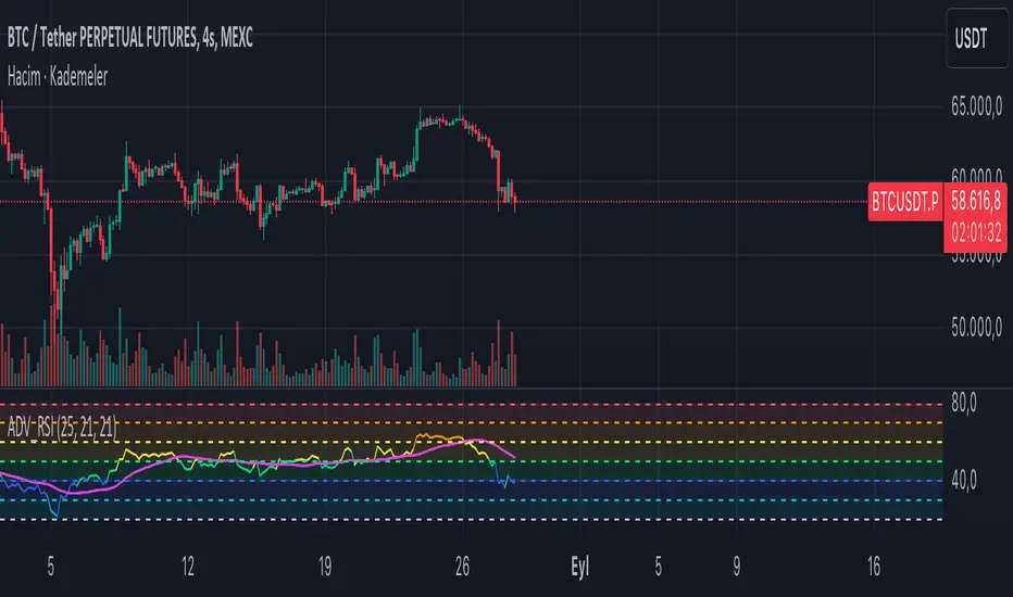
ADV_RSIADV_RSI - Advanced Relative Strength Index
Description: The ADV_RSI indicator is an advanced and mutated version of the classic Relative Strength Index (RSI), enhanced with multiple moving averages and a dynamic color-coding system. It provides traders with deeper insights into market momentum and potential trend reversals by incorporating two different moving averages of the RSI (21, and 50 periods). The indicator helps to visualize overbought and oversold conditions more effectively and offers a clear, color-coded representation of the RSI value relative to key thresholds.
Features:
RSI Calculation: The core of the indicator is based on the traditional RSI, calculated over a customizable period.
Multiple Moving Averages: The script includes two RSI moving averages (21, and 50 periods) to help identify trend strength and potential reversal points.
Dynamic RSI Color Coding: The RSI line is color-coded based on its value, ranging from red for overbought conditions to aqua for oversold conditions. This makes it easier to interpret the market's momentum at a glance.
Threshold Bands: The indicator includes horizontal threshold lines at key RSI levels (20, 30, 40, 50, 60, 70, 80), with shaded areas between them, providing a visual aid to quickly identify overbought and oversold zones.
How to Use:
The RSI line fluctuates between 0 and 100, with traditional overbought and oversold levels set at 70 and 30, respectively.
When the RSI crosses above the 70 level, it may indicate overbought conditions, signaling a potential selling opportunity.
When the RSI falls below the 30 level, it may indicate oversold conditions, signaling a potential buying opportunity.
The included moving averages of the RSI can help confirm trend direction and potential reversals.
The color coding of the RSI line provides a quick visual cue for momentum changes.
Ideal For:
Traders looking for a more nuanced understanding of market momentum.
Those who prefer visual aids for quick decision-making in identifying overbought and oversold conditions.
Traders who utilize multiple timeframes and need a comprehensive RSI tool for better accuracy in their analysis.
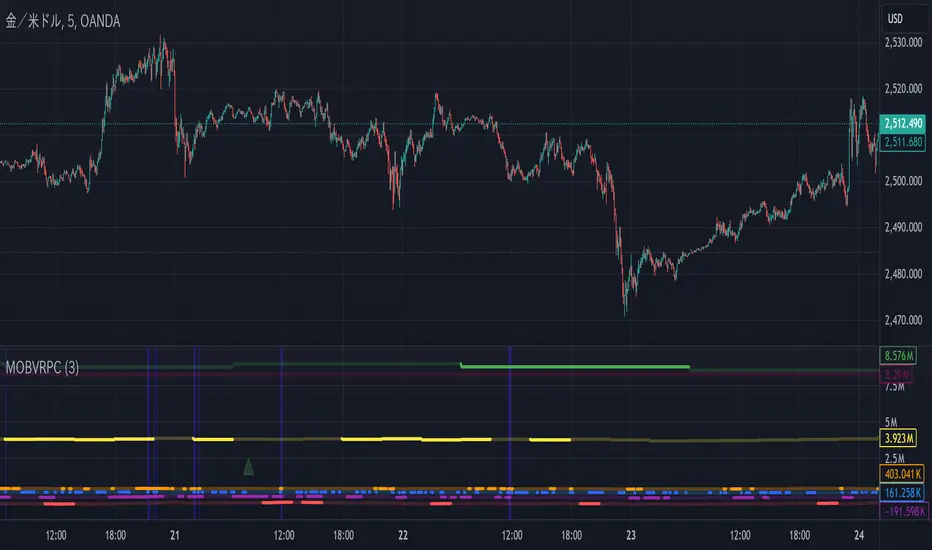
MTOBVR_CheckOverview.
This indicator checks to see if the OBV follows a specific pattern and visually displays the trend of the OBV on different time legs. It also has the ability to set alerts when certain conditions are met.
How to use
Setting up the indicator
Add a new indicator on a chart in TradingView.
Copy the code into the “Pine Script™ Editor” and save it as a new script.
Apply the script to your chart.
Indicator Functions
OBV Calculation
Calculates OBV for each time frame (5-minute, 15-minute, 30-minute, 1-hour, 4-hour, daily, and weekly) and displays it on the chart OBV is an indicator that combines price changes and trading volume.
Pattern Detection
Detects whether a particular pattern, such as a double or triple bottom, appears in the OBV. This allows us to identify buy or sell signals.
When these patterns are detected, the background color changes.
Background Color Change
When an OBV forms a particular pattern, the background color of the chart changes. This provides visual confirmation that a pattern has appeared.
Minimum pattern (min_bool): when the 5-, 15-, and 30-minute conditions for OBV are met.
High hourly pattern (h_bool): when the condition is met for the 1-hour, 4-hour, and daily legs of the OBV.
One-week pattern (range_obv_1w_bool): when the condition is met for the 1-week OBV pattern.
When all conditions are met: when the minimum pattern, high hourly pattern, and one-week pattern are all met.
Alert Settings
You can set alerts when certain conditions are met. This allows you to receive signals in real time.
Minimum conditions (min_bool): conditions at 5, 15, and 30 minutes of OBV.
High timeframe condition (h_bool): condition on the 1-hour, 4-hour, and daily legs of the OBV.
When all conditions are met: When all of the above conditions are met.
One-week condition (range_obv_1w_bool): Condition for the one-week leg of the OBV.
When all conditions are met: when the minimum, high time leg, and one week conditions are all met.
Arrows
OBV_ALL_UP: A green triangle arrow is displayed when the OBV is rising on all time legs.
OBV_ALL_DOWN: A red triangle arrow appears when the OBV is falling on all time legs.
Usage Notes
Time Leg Settings: This script uses OBVs of different time legs to detect patterns. Depending on the time leg used, appropriate settings and interpretation are required.
Alert settings: In order to activate the alert function, the alert conditions and notification method must be configured using TradingView's alert system.
This indicator allows you to visually see trends and patterns in the OBV across multiple time frames, allowing you to make more informed trading decisions.
Control Candle Range [UkutaLabs]Control Candle Range
█ OVERVIEW
The Control Candle Range is a powerful trading tool that automatically identifies control candles in real time. The versatile ranges drawn by this indicator can be used in a variety of trading strategies because they can be used as ranges as well as areas of support and resistance.
The purpose of this script is to simplify the trading experience of users by automatically identifying and displaying Control Candle Ranges.
█ USAGE
A Control Candle is a candle that is followed by two consecutive inside candles. When this pattern is detected, this indicator will automatically identify it and draw a range in real time. This range will continue to extend as long as candles continue to close within the range of the Control Candle. It is important to note that a Control Candle is still valid if the price action exits its range as long as it closes within its range.
This script also supports higher time frame mapping, allowing you to draw Control Candle Ranges from higher timeframes onto lower timeframe charts. This is a powerful feature that allows users to see multiple timeframes worth of information at a glance on one single chart.
Each Control Candle Range will also be displayed with a label to allow users to understand at a glance which timeframe the range is being drawn from. These labels can be turned off in the settings.
The user also has the ability to adjust the color of each timeframe’s ranges.
█ SETTINGS
Configuration
• Show Labels: Determines whether or not identifying labels are displayed on ranges.
• Label Size: Determines the size of labels.
• Text Alignment: Determines where labels are drawn on ranges.
• Max Display: Determines the maximum number of ranges that can be drawn from each timeframe.
Current Timeframe
• Display (On/Off): Determines whether or not ranges from the current timeframe will be drawn on the chart.
• Color: Determines the color of ranges drawn from the current timeframe.
5 Minute (Higher Timeframe)
• Display (On/Off): Determines whether or not ranges from the 5 minute timeframe will be drawn on the chart.
• Color: Determines the color of ranges drawn from the 5 minute timeframe.
15 Minute (Higher Timeframe)
• Display (On/Off): Determines whether or not ranges from the 15 minute timeframe will be drawn on the chart.
• Color: Determines the color of ranges drawn from the 15 minute timeframe.
30 Minute (Higher Timeframe)
• Display (On/Off): Determines whether or not ranges from the 30 minute timeframe will be drawn on the chart.
• Color: Determines the color of ranges drawn from the 30 minute timeframe.
60 Minute (Higher Timeframe)
• Display (On/Off): Determines whether or not ranges from the 60 minute timeframe will be drawn on the chart.
• Color: Determines the color of ranges drawn from the 60 minute timeframe.
240 Minute (Higher Timeframe)
• Display (On/Off): Determines whether or not ranges from the 240 minute timeframe will be drawn on the chart.
• Color: Determines the color of ranges drawn from the 240 minute timeframe.
Daily (Higher Timeframe)
• Display (On/Off): Determines whether or not ranges from the daily timeframe will be drawn on the chart.
• Color: Determines the color of ranges drawn from the daily timeframe.

ICT KillZones + Pivot Points [TradingFinder] Support/Resistance 🟣 Introduction
Pivot Points are critical levels on a price chart where trading activity is notably high. These points are derived from the prior day's price data and serve as key reference markers for traders' decision-making processes.
Types of Pivot Points :
Floor
Woodie
Camarilla
Fibonacci
🔵 Floor Pivot Points
Widely utilized in technical analysis, floor pivot points are essential in identifying support and resistance levels. The central pivot point (PP) acts as the primary level, suggesting the trend's likely direction.
The additional resistance levels (R1, R2, R3) and support levels (S1, S2, S3) offer further insight into potential trend reversals or continuations.
🔵 Camarilla Pivot Points
Featuring eight distinct levels, Camarilla pivot points closely correspond with support and resistance, making them highly effective for setting stop-loss orders and profit targets.
🔵 Woodie Pivot Points
Similar to floor pivot points, Woodie pivot points differ by placing greater emphasis on the closing price, often resulting in different pivot levels compared to the floor method.
🔵 Fibonacci Pivot Points
Fibonacci pivot points combine the standard floor pivot points with Fibonacci retracement levels applied to the previous trading period's range. Common retracement levels used are 38.2%, 61.8%, and 100%.
🟣 Sessions
Financial markets are divided into specific time segments, known as sessions, each with unique characteristics and activity levels. These sessions are active at different times throughout the day.
The primary sessions in financial markets include :
Asian Session
European Session
New York Session
The timing of these major sessions in UTC is as follows :
Asian Session: 23:00 to 06:00
European Session: 07:00 to 14:25
New York Session: 14:30 to 22:55
🟣 Kill Zones
Kill zones are periods within a session marked by heightened trading activity. During these times, trading volume surges and price movements become more pronounced.
The timing of the major kill zones in UTC is :
Asian Kill Zone: 23:00 to 03:55
European Kill Zone: 07:00 to 09:55
New York Kill Zone: 14:30 to 16:55
Combining kill zones and pivot points in financial market analysis provides several advantages :
Enhanced Market Sentiment Analysis : Aligns key price levels with high-activity periods for a clearer market sentiment.
Improved Timing for Trade Entries and Exits : Helps better time trades based on when price movements are most likely.
Higher Probability of Successful Trades : Increases the accuracy of predicting market movements and placing profitable trades.
Strategic Stop-Loss and Profit Target Placement : Allows for precise risk management by strategically setting stop-loss and profit targets.
Versatility Across Different Time Frames : Effective in both short and long time frames, suitable for various trading strategies.
Enhanced Trend Identification and Confirmation : Confirms trends using both pivot levels and high-activity periods, ensuring stronger trend validation.
In essence, this integrated approach enhances decision-making, optimizes trading performance, and improves risk management.
🟣 How to Use
🔵 Two Approaches to Trading Pivot Points
There are two main strategies for trading pivot points: utilizing "pivot point breakouts" and "price reversals."
🔵 Pivot Point Breakout
When the price breaks through pivot lines, it signals a shift in market sentiment to the trader. In the case of an upward breakout, where the price crosses these pivot lines, a trader might enter a long position, placing their stop-loss just below the pivot point (P).
Conversely, if the price breaks downward, a short position can be initiated below the pivot point. When using the pivot point breakout strategy, the first and second support levels can serve as profit targets in an upward trend. In a downward trend, these roles are filled by the first and second resistance levels.
🔵 Price Reversal
An alternative method involves waiting for the price to reverse at the support and resistance levels. To implement this strategy, traders should take positions opposite to the prevailing trend as the price rebounds from the pivot point.
While this tool is commonly used in higher time frames, it tends to produce better results in shorter time frames, such as 1-hour, 30-minute, and 15-minute intervals.
Three Strategies for Trading the Kill Zone
There are three principal strategies for trading within the kill zone :
Kill Zone Hunt
Breakout and Pullback to Kill Zone
Trading in the Trend of the Kill Zone
🔵 Kill Zone Hunt
This strategy involves waiting until the kill zone concludes and its high and low lines are established. If the price reaches one of these lines within the same session and is strongly rejected, a trade can be executed.
🔵 Breakout and Pullback to Kill Zone
In this approach, once the kill zone ends and its high and low lines stabilize, a trade can be made if the price breaks one of these lines decisively within the same session and then pulls back to that level.
🔵 Trading in the Trend of the Kill Zone
Kill zones are characterized by high trading volumes and strong trends. Therefore, trades can be placed in the direction of the prevailing trend. For instance, if an upward trend dominates this area, a buy trade can be entered when the price reaches a demand order block.

TASC 2024.06 REIT ETF Trading System█ OVERVIEW
This strategy script demonstrates the application of the Real Estate Investment Trust (REIT) ETF trading system presented in the article by Markos Katsanos titled "Is The Price REIT?" from TASC's June 2024 edition of Traders' Tips .
█ CONCEPTS
REIT stocks and ETFs offer a simplified, diversified approach to real estate investment. They exhibit sensitivity to interest rates, often moving inversely to interest rate and treasury yield changes. Markos Katsanos explores this relationship and the correlation of prices with the broader market to develop a trading strategy for REIT ETFs.
The script employs Bollinger Bands and Donchian channel indicators to identify oversold conditions and trends in REIT ETFs. It incorporates the 10-year treasury yield index (TNX) as a proxy for interest rates and the S&P 500 ETF (SPY) as a benchmark for the overall market. The system filters trade entries based on their behavior and correlation with the REIT ETF price.
█ CALCULATIONS
The strategy initiates long entries (buy signals) under two conditions:
1. Oversold condition
The weekly ETF low price dips below the 15-week Bollinger Band bottom, the closing price is above the value by at least 0.2 * ATR ( Average True Range ), and the price exceeds the week's median.
Either of the following:
– The TNX index is down over 15% from its 25-week high, and its correlation with the ETF price is less than 0.3.
– The yield is below 2%.
2. Uptrend
The weekly ETF price crosses above the previous week's 30-week Donchian channel high.
The SPY ETF is above its 20-week moving average.
Either of the following:
– Over ten weeks have passed since the TNX index was at its 30-week high.
– The correlation between the TNX value and the ETF price exceeds 0.3.
– The yield is below 2%.
The strategy also includes three exit (sell) rules:
1. Trailing (Chandelier) stop
The weekly close drops below the highest close over the last five weeks by over 1.5 * ATR.
The TNX value rises over the latest 25 weeks, with a yield exceeding 4%, or its value surges over 15% above the 25-week low.
2. Stop-loss
The ETF's price declines by at least 8% of the previous week's close and falls below the 30-week moving average.
The SPY price is down by at least 8%, or its correlation with the ETF's price is negative.
3. Overbought condition
The ETF's value rises above the 100-week low by over 50%.
The ETF's price falls over 1.5 * ATR below the 3-week high.
The ETF's 10-week Stochastic indicator exceeds 90 within the last three weeks.
█ DISCLAIMER
This strategy script educates users on the system outlined by the TASC article. However, note that its default properties might not fully represent real-world trading conditions for an individual. By default, it uses 10% of equity as the order size and a slippage amount of 5 ticks. Traders should adjust these settings and the commission amount when using this script. Additionally, since this strategy utilizes compound conditions on weekly data to trigger orders, it will generate significantly fewer trades than other, higher-frequency strategies.

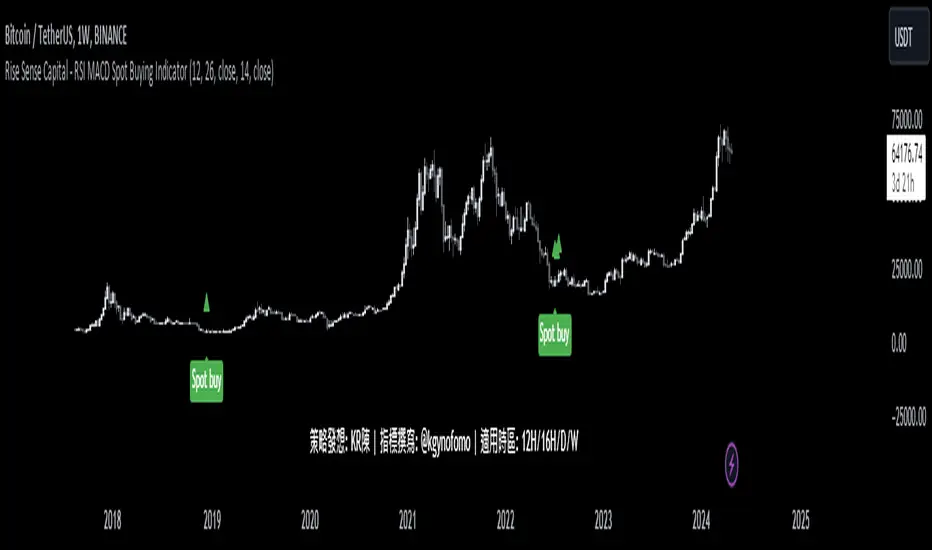
Rise Sense Capital - RSI MACD Spot Buying IndicatorToday, I'll share a spot buying strategy shared by a member @KR陳 within the DATA Trader Alliance Alpha group. First, you need to prepare two indicators:
今天分享一個DATA交易者聯盟Alpha群組裏面的群友@KR陳分享的現貨買入策略。
首先需要準備兩個指標
RSI Indicator (Relative Strength Index) - RSI is a technical analysis tool based on price movements over a period of time to evaluate the speed and magnitude of price changes. RSI calculates the changes in price over a period to determine whether the recent trend is relatively strong (bullish) or weak (bearish).
RSI指標,(英文全名:Relative Strength Index),中文稱為「相對強弱指標」,是一種以股價漲跌為基礎,在一段時間內的收盤價,用於評估價格變動的速度 (快慢) 與變化 (幅度) 的技術分析工具,RSI藉由計算一段期間內股價的漲跌變化,判斷最近的趨勢屬於偏強 (偏多) 還是偏弱 (偏空)。
MACD Indicator (Moving Average Convergence & Divergence) - MACD is a technical analysis tool proposed by Gerald Appel in the 1970s. It is commonly used in trading to determine trend reversals by analyzing the convergence and divergence of fast and slow lines.
MACD 指標 (Moving Average Convergence & Divergence) 中文名為平滑異同移動平均線指標,MACD 是在 1970 年代由美國人 Gerald Appel 所提出,是一項歷史悠久且經常在交易中被使用的技術分析工具,原理是利用快慢線的交錯,藉以判斷股價走勢的轉折。
In MACD analysis, the most commonly used values are 12, 26, and 9, known as MACD (12,26,9). The market often uses the MACD indicator to determine the future direction of assets and to identify entry and exit points.
在 MACD 的技術分析中,最常用的值為 12 天、26 天、9 天,也稱為 MACD (12,26,9),市場常用 MACD 指標來判斷操作標的的後市走向,確定波段漲幅並找到進、出場點。
Strategy analysis by member KR陳:
策略解析 by群友 KR陳 :
Condition 1: RSI value in the previous candle is below oversold zone(30).
條件1:RSI 在前一根的數值低於超賣區(30)
buycondition1 = RSI <30
Condition 2: MACD histogram changes from decreasing to increasing.
條件2:MACD柱由遞減轉遞增
buycondition2 = hist >hist and hist
MTF Trend Truth [Hubka]A Multi Time Frame Tend table that displays symbols trends for 6 selectable Time Intervals. In addition to the 6 first row color trends, the table also displays the direction of the last 2 candles in each Time Interval in the last 2 rows. This extra interval information displays price trend direction change or may add confluence if the price direction is the same.
The top row of the table has column header names described below:
(TL30) Column 1 - Trend Interval + The Trend Length selected (30 is default). Uses the last 30 candles to determine the trend for this interval. The length number is Editable.
(LCC) Column 2 - Last Closed Candle. This is the direction color of the second last candle on the chart.
(LOC) Column 3 - Last Open Candle. The is the current candle color direction of the last candle on the chart. This candle has not yet closed and will flicker as price changing state.
NOTE 1: (LOC) Column 3 - Last Open Candle - only displays correctly when the market is open and price is changing.
You can adjust the "Trend Length in Candles" which defaults to using the trend of the last 30 candles (TL30). Edit this setting to use any number from 5 to 99 candles back if you want display different trend lengths.
Having a visual table of the price trends from different time intervals can be beneficial to traders. For example... When observing that a symbol has many Bullish (green) price trends on several time intervals and the last 2 candles are also bullish it should afford a trader confluence to trade in that same bullish direction. However I am not a professional and do not offer any trading advice in any way. Use this indicator at your own risk.
NOTE 2: Time interval of 240 = 4 hours. Below 1 day number only is minutes.
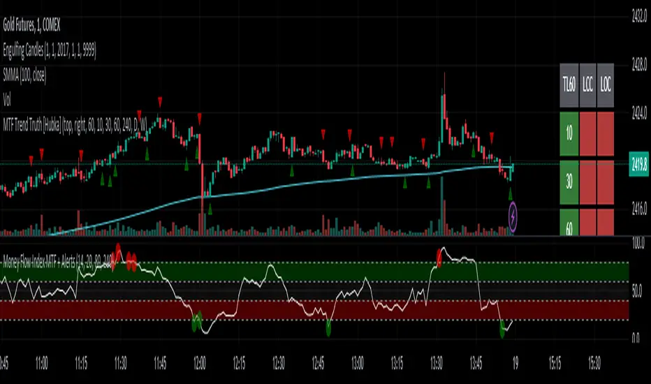
GG - LevelsThe GG Levels indicator is a tool designed for day trading U.S. equity futures. It highlights key levels intraday, overnight, intermediate-swing levels that are relevant for intraday futures trading.
Terminology
RTH (Regular Trading Hours): Represents the New York session from 09:30 to 17:00 EST.
ON Session (Overnight Session): Represents the trading activity from 17:00 to 09:29 EST.
IB (Initial Balance): The first hour of the New York session, from 09:30 to 10:30 EST.
Open: The opening price of the RTH session.
YH (Yesterday's High): The highest price during the RTH session of the previous day.
YL (Yesterday's Low): The lowest price during the RTH session of the previous day.
YC (Yesterday's Close): The daily bar close which for futures gets updated to settlement.
IBH (Initial Balance High): The highest price during the IB session.
IBL (Initial Balance Low): The lowest price during the IB session.
ONH (Overnight High): The highest price during the ON session.
ONL (Overnight Low): The lowest price during the ON session.
VWAP (Volume-Weighted Average Price): The volume-weighted average price that resets each day.
Why is RTH Important?
Tracking the RTH session is important because often times the overnight session can be filled with "lies". It is thought that because the overnight session is lower volume price can be pushed or "manipulated" to extremes that would not happen during higher volume times.
Why is the ON Session Important Then?
Just because the ON session can be thought as a "lie" doesn't mean it is relevant to know. For example, if price is stuck inside the ON range then you can think of the market as rotational or range-bound. If price is above the ON range then it can be thought of as bullish. If price is below the ON range then it can be thought as bearish.
What is IB?
IB or initial balance is the first hour of the New York Session. Typically the market sets the tone for the day in the first hour. This tone is similarly a map like the ON session. If we are above the IBH then it is bullish and likely a trend day to the upside. If we are below the IBL then it is bearish and likely a trend day to the downside. If we are in IB then we want to avoid conducting business in the middle of IBH and IBL to avoid getting chopped up in a range bound market.
These levels are not a holy grail
You should use this indicator as guide or map for context about the instrument you are trading. You need to combine your own technical analysis with this indicator. You want as much context confirming your trade thesis in order to enter a trade. Simply buying or selling because we are above or below a level is not recommended in any circumstance. If it were that easy I would not publish this indicator.
Adjustments
In the indicator settings you can adjust the RTH, ON, and IB session-time settings. All of the times entered must be in EST (Eastern Standard Time). You may want to do this to apply the levels to a foreign market.
Examples

Trend Change IndicatorThe Trend Change Indicator is an all-in-one, user-friendly trend-following tool designed to identify bullish and bearish trends in asset prices. It features adjustable input values and a built-in alert system that promptly notifies investors of potential shifts in both short-term and long-term price trends. This alert system is crucial for helping less active investors correctly position themselves ahead of major trend shifts and assists in risk management after a trend is established. It's important to note that this indicator is most effective with assets that historically exhibit strong trends.
At the heart of this tool is the interaction between the 30-day and 60-day Exponential Moving Averages (EMA). A bullish trend is indicated in green when the 30-day EMA is above the 60-day EMA, while a bearish trend is signaled in red when the 30-day EMA is below the 60-day EMA. The appearance of gray alerts users to potential shifts in the current trend as the EMAs converge, falling below the Average True Range (ATR) safety margin. This analysis is conducted across both hourly and daily timeframes, with the 4-hour timeframe providing early signals for daily trend changes. The band visually represents the interaction between the daily EMAs and is also displayed in the second row of the table, with the first row showing the same EMA interaction on the 4-hour timeframe.
This indicator also includes a 140-day (20-week) Simple Moving Average (SMA), visually represented by a line with predictive dots. This feature significantly enhances the investor's ability to understand long-term trends in asset prices, offering forward-looking insights by projecting the SMA value 10 days into the future. The value of this forecast lies in interpreting the slope of the dots; upward trending dots suggest a bullish underlying trend, while downward trending dots indicate a bearish trend. Generally, prices above the SMA signal bullishness, and prices below indicate bearishness.
In summary, the Trend Change Indicator is a comprehensive solution for identifying price trends and managing risk. Its intuitive, color-coded design makes it an indispensable tool for traders and investors who aim to be well-positioned ahead of trend shifts and manage risk once a trend has been established. While it has proven historically valuable in trending markets such as cryptocurrencies, tech stocks, and commodities, it is advisable to use this indicator in conjunction with other technical analysis tools for a more comprehensive and well-rounded decision-making process.

Time Matrix TableICT stresses time and liquidity levels in his teachings. This table helps to easily locate these key Time-based price levels. You can use these levels to determine your directional bias and to help generate your narrative for where the market is going.
This indicator creates a table that gives you the price for the following liquidity levels:
PDO - Previous Day Open
PDH - Previous Day High
PDL - Previous Day Low
PDC - Previous Day Close
PDEQ - Equilibrium of the previous day's range. (Calculated by math.abs(((pdh-pdl)/2)+pdl))
PWH - Previous Week High
PWL - Previous Week Low
PDH2 - Two Days Back High
PDL2 - Two Days Back Low
PDH3 - Three Days Back High
PDL3 - Three Days Back Low
And gives you the opening price for the following times:
Daily Open - 6:00pm open for current session
1:30 AM
3:00 AM
4:00 AM
Midnight Open
6:00 AM
7:30 AM
8:30 AM
NY Open
10:00 AM
12:00 PM
NY PM - 1:30pm
2:00 PM
The levels are sorted descending in price in the table, with the background colored based on their relation to price. The prices are also plotted on the chart based on the range you specify in relation to the current price. These lines are also colored based on their relation to price.
This indicator does not give you anything but the price at a specific time, you must determine your own bias and narrative based on the levels that are given.
