S&P 100 Option Expiration Week StrategyThe Option Expiration Week Strategy aims to capitalize on increased volatility and trading volume that often occur during the week leading up to the expiration of options on stocks in the S&P 100 index. This period, known as the option expiration week, culminates on the third Friday of each month when stock options typically expire in the U.S. During this week, investors in this strategy take a long position in S&P 100 stocks or an equivalent ETF from the Monday preceding the third Friday, holding until Friday. The strategy capitalizes on potential upward price pressures caused by increased option-related trading activity, rebalancing, and hedging practices.
The phenomenon leveraged by this strategy is well-documented in finance literature. Studies demonstrate that options expiration dates have a significant impact on stock returns, trading volume, and volatility. This effect is driven by various market dynamics, including portfolio rebalancing, delta hedging by option market makers, and the unwinding of positions by institutional investors (Stoll & Whaley, 1987; Ni, Pearson, & Poteshman, 2005). These market activities intensify near option expiration, causing price adjustments that may create short-term profitable opportunities for those aware of these patterns (Roll, Schwartz, & Subrahmanyam, 2009).
The paper by Johnson and So (2013), Returns and Option Activity over the Option-Expiration Week for S&P 100 Stocks, provides empirical evidence supporting this strategy. The study analyzes the impact of option expiration on S&P 100 stocks, showing that these stocks tend to exhibit abnormal returns and increased volume during the expiration week. The authors attribute these patterns to intensified option trading activity, where demand for hedging and arbitrage around options expiration causes temporary price adjustments.
Scientific Explanation
Research has found that option expiration weeks are marked by predictable increases in stock returns and volatility, largely due to the role of options market makers and institutional investors. Option market makers often use delta hedging to manage exposure, which requires frequent buying or selling of the underlying stock to maintain a hedged position. As expiration approaches, their activity can amplify price fluctuations. Additionally, institutional investors often roll over or unwind positions during expiration weeks, creating further demand for underlying stocks (Stoll & Whaley, 1987). This increased demand around expiration week typically leads to temporary stock price increases, offering profitable opportunities for short-term strategies.
Key Research and Bibliography
Johnson, T. C., & So, E. C. (2013). Returns and Option Activity over the Option-Expiration Week for S&P 100 Stocks. Journal of Banking and Finance, 37(11), 4226-4240.
This study specifically examines the S&P 100 stocks and demonstrates that option expiration weeks are associated with abnormal returns and trading volume due to increased activity in the options market.
Stoll, H. R., & Whaley, R. E. (1987). Program Trading and Expiration-Day Effects. Financial Analysts Journal, 43(2), 16-28.
Stoll and Whaley analyze how program trading and portfolio insurance strategies around expiration days impact stock prices, leading to temporary volatility and increased trading volume.
Ni, S. X., Pearson, N. D., & Poteshman, A. M. (2005). Stock Price Clustering on Option Expiration Dates. Journal of Financial Economics, 78(1), 49-87.
This paper investigates how option expiration dates affect stock price clustering and volume, driven by delta hedging and other option-related trading activities.
Roll, R., Schwartz, E., & Subrahmanyam, A. (2009). Options Trading Activity and Firm Valuation. Journal of Financial Markets, 12(3), 519-534.
The authors explore how options trading activity influences firm valuation, finding that higher options volume around expiration dates can lead to temporary price movements in underlying stocks.
Cao, C., & Wei, J. (2010). Option Market Liquidity and Stock Return Volatility. Journal of Financial and Quantitative Analysis, 45(2), 481-507.
This study examines the relationship between options market liquidity and stock return volatility, finding that increased liquidity needs during expiration weeks can heighten volatility, impacting stock returns.
Summary
The Option Expiration Week Strategy utilizes well-researched financial market phenomena related to option expiration. By positioning long in S&P 100 stocks or ETFs during this period, traders can potentially capture abnormal returns driven by option market dynamics. The literature suggests that options-related activities—such as delta hedging, position rollovers, and portfolio adjustments—intensify demand for underlying assets, creating short-term profit opportunities around these key dates.
Cerca negli script per "沪深主板45度上升的股票"

Payday Anomaly StrategyThe "Payday Effect" refers to a predictable anomaly in financial markets where stock returns exhibit significant fluctuations around specific pay periods. Typically, these are associated with the beginning, middle, or end of the month when many investors receive wages and salaries. This influx of funds, often directed automatically into retirement accounts or investment portfolios (such as 401(k) plans in the United States), temporarily increases the demand for equities. This phenomenon has been linked to a cycle where stock prices rise disproportionately on and around payday periods due to increased buy-side liquidity.
Academic research on the payday effect suggests that this pattern is tied to systematic cash flows into financial markets, primarily driven by employee retirement and savings plans. The regularity of these cash infusions creates a calendar-based pattern that can be exploited in trading strategies. Studies show that returns on days around typical payroll dates tend to be above average, and this pattern remains observable across various time periods and regions.
The rationale behind the payday effect is rooted in the behavioral tendencies of investors, specifically the automatic reinvestment mechanisms used in retirement funds, which align with monthly or semi-monthly salary payments. This regular injection of funds can cause market microstructure effects where stock prices temporarily increase, only to stabilize or reverse after the funds have been invested. Consequently, the payday effect provides traders with a potentially profitable opportunity by predicting these inflows.
Scientific Bibliography on the Payday Effect
Ma, A., & Pratt, W. R. (2017). Payday Anomaly: The Market Impact of Semi-Monthly Pay Periods. Social Science Research Network (SSRN).
This study provides a comprehensive analysis of the payday effect, exploring how returns tend to peak around payroll periods due to semi-monthly cash flows. The paper discusses how systematic inflows impact returns, leading to predictable stock performance patterns on specific days of the month.
Lakonishok, J., & Smidt, S. (1988). Are Seasonal Anomalies Real? A Ninety-Year Perspective. The Review of Financial Studies, 1(4), 403-425.
This foundational study explores calendar anomalies, including the payday effect. By examining data over nearly a century, the authors establish a framework for understanding seasonal and monthly patterns in stock returns, which provides historical support for the payday effect.
Owen, S., & Rabinovitch, R. (1983). On the Predictability of Common Stock Returns: A Step Beyond the Random Walk Hypothesis. Journal of Business Finance & Accounting, 10(3), 379-396.
This paper investigates predictability in stock returns beyond random fluctuations. It considers payday effects among various calendar anomalies, arguing that certain dates yield predictable returns due to regular cash inflows.
Loughran, T., & Schultz, P. (2005). Liquidity: Urban versus Rural Firms. Journal of Financial Economics, 78(2), 341-374.
While primarily focused on liquidity, this study provides insight into how cash flows, such as those from semi-monthly paychecks, influence liquidity levels and consequently impact stock prices around predictable pay dates.
Ariel, R. A. (1990). High Stock Returns Before Holidays: Existence and Evidence on Possible Causes. The Journal of Finance, 45(5), 1611-1626.
Ariel’s work highlights stock return patterns tied to certain dates, including paydays. Although the study focuses on pre-holiday returns, it suggests broader implications of predictable investment timing, reinforcing the calendar-based effects seen with payday anomalies.
Summary
Research on the payday effect highlights a repeating pattern in stock market returns driven by scheduled payroll investments. This cyclical increase in stock demand aligns with behavioral finance insights and market microstructure theories, offering a valuable basis for trading strategies focused on the beginning, middle, and end of each month.

Futures Beta Overview with Different BenchmarksBeta Trading and Its Implementation with Futures
Understanding Beta
Beta is a measure of a security's volatility in relation to the overall market. It represents the sensitivity of the asset's returns to movements in the market, typically benchmarked against an index like the S&P 500. A beta of 1 indicates that the asset moves in line with the market, while a beta greater than 1 suggests higher volatility and potential risk, and a beta less than 1 indicates lower volatility.
The Beta Trading Strategy
Beta trading involves creating positions that exploit the discrepancies between the theoretical (or expected) beta of an asset and its actual market performance. The strategy often includes:
Long Positions on High Beta Assets: Investors might take long positions in assets with high beta when they expect market conditions to improve, as these assets have the potential to generate higher returns.
Short Positions on Low Beta Assets: Conversely, shorting low beta assets can be a strategy when the market is expected to decline, as these assets tend to perform better in down markets compared to high beta assets.
Betting Against (Bad) Beta
The paper "Betting Against Beta" by Frazzini and Pedersen (2014) provides insights into a trading strategy that involves betting against high beta stocks in favor of low beta stocks. The authors argue that high beta stocks do not provide the expected return premium over time, and that low beta stocks can yield higher risk-adjusted returns.
Key Points from the Paper:
Risk Premium: The authors assert that investors irrationally demand a higher risk premium for holding high beta stocks, leading to an overpricing of these assets. Conversely, low beta stocks are often undervalued.
Empirical Evidence: The paper presents empirical evidence showing that portfolios of low beta stocks outperform portfolios of high beta stocks over long periods. The performance difference is attributed to the irrational behavior of investors who overvalue riskier assets.
Market Conditions: The paper suggests that the underperformance of high beta stocks is particularly pronounced during market downturns, making low beta stocks a more attractive investment during volatile periods.
Implementation of the Strategy with Futures
Futures contracts can be used to implement the betting against beta strategy due to their ability to provide leveraged exposure to various asset classes. Here’s how the strategy can be executed using futures:
Identify High and Low Beta Futures: The first step involves identifying futures contracts that have high beta characteristics (more sensitive to market movements) and those with low beta characteristics (less sensitive). For example, commodity futures like crude oil or agricultural products might exhibit high beta due to their price volatility, while Treasury bond futures might show lower beta.
Construct a Portfolio: Investors can construct a portfolio that goes long on low beta futures and short on high beta futures. This can involve trading contracts on stock indices for high beta stocks and bonds for low beta exposures.
Leverage and Risk Management: Futures allow for leverage, which means that a small movement in the underlying asset can lead to significant gains or losses. Proper risk management is essential, using stop-loss orders and position sizing to mitigate the inherent risks associated with leveraged trading.
Adjusting Positions: The positions may need to be adjusted based on market conditions and the ongoing performance of the futures contracts. Continuous monitoring and rebalancing of the portfolio are essential to maintain the desired risk profile.
Performance Evaluation: Finally, investors should regularly evaluate the performance of the portfolio to ensure it aligns with the expected outcomes of the betting against beta strategy. Metrics like the Sharpe ratio can be used to assess the risk-adjusted returns of the portfolio.
Conclusion
Beta trading, particularly the strategy of betting against high beta assets, presents a compelling approach to capitalizing on market inefficiencies. The research by Frazzini and Pedersen emphasizes the benefits of focusing on low beta assets, which can yield more favorable risk-adjusted returns over time. When implemented using futures, this strategy can provide a flexible and efficient means to execute trades while managing risks effectively.
References
Frazzini, A., & Pedersen, L. H. (2014). Betting against beta. Journal of Financial Economics, 111(1), 1-25.
Fama, E. F., & French, K. R. (1992). The cross-section of expected stock returns. Journal of Finance, 47(2), 427-465.
Black, F. (1972). Capital Market Equilibrium with Restricted Borrowing. Journal of Business, 45(3), 444-454.
Ang, A., & Chen, J. (2010). Asymmetric volatility: Evidence from the stock and bond markets. Journal of Financial Economics, 99(1), 60-80.
By utilizing the insights from academic literature and implementing a disciplined trading strategy, investors can effectively navigate the complexities of beta trading in the futures market.

ICT MACROS (UTC-4)This Pine Script creates an indicator that draws vertical lines on a TradingView chart to mark specific time intervals during the day. It allows the user to see when certain predefined time periods start and end, using vertical lines of different colors. The script is designed to work with time frames aligned to the UTC-4 timezone.
### Key Features of the Script
1. **Vertical Line Drawing Function**:
- The script uses a custom function, `draw_vertical_line`, to draw vertical lines at specific times.
- This function takes four parameters:
- `specificTime`: The specific timestamp when the vertical line should be drawn.
- `lineColor`: The color of the vertical line.
- `labelText`: The text label for the line (used internally for debugging purposes).
- `adjustment_minutes`: An integer value that allows time adjustment (in minutes) to make the lines align more accurately with the chart’s candles.
- The function calculates an adjusted time using the `adjustment_minutes` parameter and checks if the current time (`time`) falls within a 3-minute range of the adjusted time. If it does, it draws a vertical line.
2. **User Input for Time Adjustment**:
- The `adjustment_minutes` input allows users to fine-tune the appearance of the lines by shifting them slightly forward or backward in time to ensure they align with the chart candles. This is useful because of potential minor discrepancies between the script’s timestamps and the chart’s actual candle times.
3. **Predefined Time Intervals**:
- The script specifies six different time intervals (using the UTC-4 timezone) and draws vertical lines to mark the start and end of each interval:
- **First interval**: 8:50 - 9:10 AM
- **Second interval**: 9:50 - 10:10 AM
- **Third interval**: 10:50 - 11:10 AM
- **Fourth interval**: 13:10 - 13:40 PM
- **Fifth interval**: 14:50 - 15:10 PM
- **Sixth interval**: 15:15 - 15:45 PM
- For each interval, there are two timestamps: the start time and the end time. The script draws a green vertical line for the start and a red vertical line for the end.
4. **Line Drawing Logic**:
- For each time interval, the script calculates the timestamp using the `timestamp()` function with the specified time in UTC-4.
- The `draw_vertical_line` function is called twice for each interval: once for the start time (with a green line) and once for the end time (with a red line).
5. **Visual Overlay**:
- The script uses the `overlay=true` setting, which means that the vertical lines are drawn directly on top of the existing price chart. This helps in visually identifying the specific time intervals without cluttering the chart.
### Summary
This Pine Script is designed for traders or analysts who want to visualize specific time intervals directly on their TradingView charts. It provides a customizable way to highlight these intervals using vertical lines, making it easier to analyze price action or trading volume during key times of the day. The `adjustment_minutes` input adds flexibility to align these lines accurately with chart data.
Grandfather-Father-Son RSI Buy Indicator-only for daily TFGrandfather-Father-Son RSI Buy and Sell Indicator
This script identifies buy and sell opportunities by combining RSI values across multiple timeframes to capture market trends and reversals. The "Grandfather-Father-Son" concept breaks down RSI analysis into three key timeframes:
Grandfather (Monthly): Represents the long-term trend, helping to filter trades that align with the overall market direction.
Father (Weekly): Provides intermediate-term momentum, confirming market conditions before signaling entry or exit points.
Son (Daily): Tracks short-term corrections and movements to pinpoint precise buy and sell opportunities.
Key Features:
Buy Signal: A buy signal is triggered when:
Monthly RSI (Grandfather) and Weekly RSI (Father) are both above 70.
Daily RSI (Son) is between 40 and 45, signaling a potential market pullback before resuming the upward trend.
The indicator checks for alignment across these timeframes to generate a reliable buy signal.
Sell Signal: A sell signal occurs when the Daily RSI (Son) crosses above 70, indicating a potential overbought condition.
Multi-Timeframe Analysis: The script pulls data from higher timeframes (monthly and weekly) to ensure that signals reflect larger market trends rather than short-term fluctuations.
Instructions:
Optimal Timeframe: This script works best on the Daily timeframe, as it uses Monthly and Weekly RSI for trend confirmation. The indicator will display a warning if applied to other timeframes to ensure it is used optimally.
Trend Alignment: The strategy ensures that buy signals are triggered only when there is a strong uptrend in both the Grandfather (Monthly) and Father (Weekly) RSI, while sell signals are based on potential overbought conditions in the Son (Daily) RSI.
Limitations:
Timeframe Dependency: Signals are based on higher timeframe data (Weekly and Monthly), which may only update at the close of those respective time periods. Therefore, it is designed to work in real-time but will be most reliable when trading in alignment with these longer-term trends.
Replay Mode: The script has been optimized to function correctly during live market conditions, with no reliance on future data (no lookahead). This ensures signals appear accurately during both backtesting and live trading.
Disclaimer:
This script is for educational purposes and should be used with caution. Always backtest before using in live trading and adjust parameters to fit your trading strategy and risk management plan.

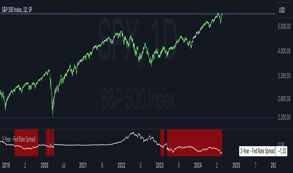
2-Year - Fed Rate SpreadThe “2-Year - Fed Rate Spread” is a financial indicator that measures the difference between the 2-Year Treasury Yield and the Federal Funds Rate (Fed Funds Rate). This spread is often used as a gauge of market sentiment regarding the future direction of interest rates and economic conditions.
Calculation
• 2-Year Treasury Yield: This is the return on investment, expressed as a percentage, on the U.S. government’s debt obligations that mature in two years.
• Federal Funds Rate: The interest rate at which depository institutions trade federal funds (balances held at Federal Reserve Banks) with each other overnight.
The indicator calculates the spread by subtracting the Fed Funds Rate from the 2-Year Treasury Yield:
{2-Year - Fed Rate Spread} = {2-Year Treasury Yield} - {Fed Funds Rate}
Interpretation:
• Positive Spread: A positive spread (2-Year Treasury Yield > Fed Funds Rate) typically suggests that the market expects the Fed to raise rates in the future, indicating confidence in economic growth.
• Negative Spread: A negative spread (2-Year Treasury Yield < Fed Funds Rate) can indicate market expectations of a rate cut, often signaling concerns about an economic slowdown or recession. When the spread turns negative, the indicator’s background turns red, making it visually easy to identify these periods.
How to Use:
• Trend Analysis: Investors and analysts can use this spread to assess the market’s expectations for future monetary policy. A persistent negative spread may suggest a cautious approach to equity investments, as it often precedes economic downturns.
• Confirmation Tool: The spread can be used alongside other economic indicators, such as the yield curve, to confirm signals about the direction of interest rates and economic activity.
Research and Academic References:
The 2-Year - Fed Rate Spread is part of a broader analysis of yield spreads and their implications for economic forecasting. Several academic studies have examined the predictive power of yield spreads, including those that involve the 2-Year Treasury Yield and Fed Funds Rate:
1. Estrella, Arturo, and Frederic S. Mishkin (1998). “Predicting U.S. Recessions: Financial Variables as Leading Indicators.” The Review of Economics and Statistics, 80(1): 45-61.
• This study explores the predictive power of various financial variables, including yield spreads, in forecasting U.S. recessions. The authors find that the yield spread is a robust leading indicator of economic downturns.
2. Estrella, Arturo, and Gikas A. Hardouvelis (1991). “The Term Structure as a Predictor of Real Economic Activity.” The Journal of Finance, 46(2): 555-576.
• The paper examines the relationship between the term structure of interest rates (including short-term spreads like the 2-Year - Fed Rate) and future economic activity. The study finds that yield spreads are significant predictors of future economic performance.
3. Rudebusch, Glenn D., and John C. Williams (2009). “Forecasting Recessions: The Puzzle of the Enduring Power of the Yield Curve.” Journal of Business & Economic Statistics, 27(4): 492-503.
• This research investigates why the yield curve, particularly spreads involving short-term rates like the 2-Year Treasury Yield, remains a powerful tool for forecasting recessions despite changes in monetary policy.
Conclusion:
The 2-Year - Fed Rate Spread is a valuable tool for market participants seeking to understand future interest rate movements and potential economic conditions. By monitoring the spread, especially when it turns negative, investors can gain insights into market sentiment and adjust their strategies accordingly. The academic research supports the use of such yield spreads as reliable indicators of future economic activity.
Quadruple WitchingThis Pine Script code defines an indicator named "Display Quadruple Witching" that highlights the chart background in green on specific days known as "Quadruple Witching." Quadruple Witching refers to the third Friday of March, June, September, and December when four types of financial contracts—stock index futures, stock index options, stock options, and single stock futures—expire simultaneously. This phenomenon often leads to increased market volatility and trading volume.
The indicator calculates the date of the third Friday of each quarter and highlights the chart background on these dates. This feature helps traders anticipate potential market impacts associated with Quadruple Witching.
Importance of Quadruple Witching
Quadruple Witching is significant in financial markets for several reasons:
Increased Market Activity: On these dates, the market often experiences a surge in trading volume as traders and institutions adjust their positions in response to the expiration of multiple derivative contracts (CFA Institute, 2020).
Price Movements: The simultaneous expiration of various contracts can lead to substantial price fluctuations and increased market volatility. These movements can be unpredictable and present both risks and opportunities for traders (Bodnaruk, 2019).
Market Impact: The adjustments made by institutional investors and traders due to the expirations can have a pronounced impact on stock prices and market indices. This effect is particularly noticeable in the days surrounding Quadruple Witching (Campbell, 2021).
References
CFA Institute. (2020). The Impact of Quadruple Witching on Financial Markets. CFA Institute Research Foundation. Retrieved from CFA Institute.
Bodnaruk, A. (2019). The Effect of Option Expiration on Stock Prices. Journal of Financial Economics, 131(1), 45-64. doi:10.1016/j.jfineco.2018.08.004
Campbell, J. Y. (2021). The Behaviour of Stock Prices Around Expiration Dates. Journal of Financial Economics, 141(2), 577-600. doi:10.1016/j.jfineco.2021.01.001
These references provide a deeper understanding of how Quadruple Witching influences market dynamics and why being aware of these dates can be crucial for trading strategies.

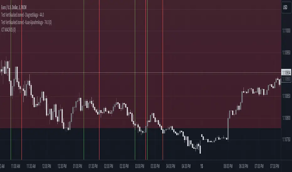
Macro Times [Blu_Ju]About ICT Macro Times:
The Inner Circle Trader (ICT) has taught that there are certain time sessions when the Interbank Price Delivery Algorithm (IPDA) is running a macro. The macro itself could be a repricing macro, a consolidation macro, etc. - this depends on where price currently is in relation to its draw. The times the macro is active do not change however, and are always the following (in New York local time):
8:50-9:10 (premarket macro)
9:50-10:10 (AM macro 1)
10:50-11:10 (AM macro 2)
11:50-12:10 (lunch macro)
13:10-13:40 (PM macro)
15:15-15:45 (final hour macro)
Because these times are fixed, traders can anticipate a setup is likely to form in or around these sessions. Setups may involve sweeps of liquidity (highs/lows), repricing to inefficiencies (e.g., fair value gaps), breaker setups, etc. (The specific setup involved is beyond the scope of this script; this script is concerned with visually marking the time sessions only.)
About this Script:
The scope of this script is to visually identify the macro active time sessions. This script draws vertical lines to mark the start and end of the macro time sessions. Optionally, the user can use a background color for the macro session with or without the vertical lines. The user can also toggle on or off any of the macro sessions, if he or she is only interested in certain ones. The user also has the freedom to change the times of the macro sessions if he or she is interested in a different time.
What makes this script unique is that it plots the macro time sessions after midnight for each day, before the real-time bar reaches the macro times. This is advantageous to the trader, as it gives the trader a visual cue that the macro times are approaching. When watching price it is easy to lose track of time, and the purpose of this script is to help the trader maintain where price is in relation to the macro time sessions in a simple, visual way.

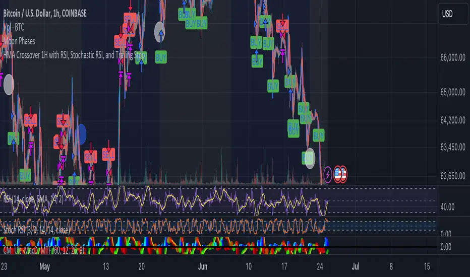
HMA Crossover 1H with RSI, Stochastic RSI, and Trailing StopThe strategy script provided is a trading algorithm designed to help traders make informed buy and sell decisions based on certain technical indicators. Here’s a breakdown of what each part of the script does and how the strategy works:
Key Components:
Hull Moving Averages (HMA):
HMA 5: This is a Hull Moving Average calculated over 5 periods. HMAs are used to smooth out price data and identify trends more quickly than traditional moving averages.
HMA 20: This is another HMA but calculated over 20 periods, providing a broader view of the trend.
Relative Strength Index (RSI):
RSI 14: This is a momentum oscillator that measures the speed and change of price movements over a 14-period timeframe. It helps identify overbought or oversold conditions in the market.
Stochastic RSI:
%K: This is the main line of the Stochastic RSI, which combines the RSI and the Stochastic Oscillator to provide a more sensitive measure of overbought and oversold conditions. It is smoothed with a 3-period simple moving average.
Trading Signals:
Buy Signal:
Generated when the 5-period HMA crosses above the 20-period HMA, indicating a potential upward trend.
Additionally, the RSI must be below 45, suggesting that the market is not overbought.
The Stochastic RSI %K must also be below 39, confirming the oversold condition.
Sell Signal:
Generated when the 5-period HMA crosses below the 20-period HMA, indicating a potential downward trend.
The RSI must be above 60, suggesting that the market is not oversold.
The Stochastic RSI %K must also be above 63, confirming the overbought condition.
Trailing Stop Loss:
This feature helps protect profits by automatically selling the position if the price moves against the trade by 5%.
For sell positions, an additional trailing stop of 100 points is included.
RSI EMA WMA (hieuhn)Indicator: RSI & EMA & WMA (14-9-45)
This indicator, named "RSI & EMA & WMA", is a versatile tool designed to provide insights into market momentum and trend strength by combining multiple technical indicators.
The Relative Strength Index (RSI) is a popular momentum oscillator used to measure the speed and change of price movements. In this indicator, RSI is plotted alongside its Exponential Moving Average (EMA) and Weighted Moving Average (WMA). EMA and WMA are smoothing techniques applied to RSI to help identify trends more clearly.
Key features of this indicator include:
RSI: The main RSI line is plotted on the chart, offering insights into overbought and oversold conditions.
EMA of RSI: The Exponential Moving Average of RSI smooths out short-term fluctuations, aiding in trend identification.
WMA of RSI: The Weighted Moving Average of RSI gives more weight to recent data points, providing a faster response to price changes.
Additionally, this indicator marks specific RSI levels considered as bullish and bearish trends, helping traders identify potential entry or exit points based on market sentiment.
By combining these technical indicators, traders can gain a comprehensive understanding of market dynamics, helping them make more informed trading decisions.

Gabriels Trend Regularity Adaptive Moving Average Dragon This is an improved version of the trend following Williams Alligator, through the use of five Trend Regularity Adaptive Moving Averages (TRAMA) instead of three smoothed averages (SMMA). This indicator can double as a TRAMA Ribbon indicator by reducing the offset to zero. Whereas the active offset can double as a forecasting indicator for options and futures.
This indicator uses five TRAMAs, set at 8, 21, 55, 144, and 233 periods. They make up the Lips, Teeth, Jaws, Wings, and Tail of the Dragon. This indicator uses convergence-divergence relationships to build trading signals, with the Tail making the slowest turns and the Lips making the fastest turns. The Lips crossing downwards through the other lines signal a short opportunity, whereas Lips crossing upwards through other lines signal a buying opportunity. The downward cross can be referred to as the Dragon "Sleeping" , and the upward cross as the Dragon "Awakening" .
In particular, but not limited to, the Wings and Tail movements possess a Roar-like forecast effect on the market. Respectively, they can be referred to as the Dragon "Spreading its Wings" or "Swinging its Tail" .
The first three lines, stretching apart and constantly moving higher or lower, denote periods in which long or short equity positions should be managed and maintained. This can be referred to as the Dragon "Eating with a mouth wide open" . Whereas indicator lines converging into narrow bands and shifting into a horizontal position can denote a trending period coming to an end, signaling the need for profit-taking and position realignment. Conversely, a previous flat line moving can denote a new trending period starting.
This indicator can double as a Multiple TRAMAs indicator by reducing the offset to zero. As such, very interesting results can be observed when used in a moving average crossover system such as the Williams Alligator or as trailing support and resistance.
The following moving average adapts to the average of the highest high and lowest low made over a specific period, thus adapting to trend strength. The TRAMA can be used like most moving averages, with the advantage of being smoother during ranging markets because it is calculated through exponential averaging.
It is calculating, using a smoothing factor, the squared simple moving average of the number of highest highs or lowest lows previously made. Where the highest highs and lowest lows are calculated using rolling maximums and minimums. Therefore, squaring allows the moving average to penalize lower values, thus appearing stationary during ranging markets.
As with all moving averages, it is still a lagging indicator, and it can suffer whipsaws when the market moves too violently or when it consolidates in ranging conditions. Despite it working in all timeframes, it won't be as formidable in the 1–5-minute scalping timeframes due to that. I would suggest 5 to 45 minutes if you are a swing trader, or hourly, daily, and weekly if you are a long-term investor.
I hope you enjoy this indicator! It's the first indicator I made, so constructive criticism would be appreciated. Thanks!
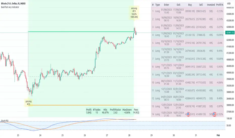
Backtest any Indicator v5Happy Trade,
here you get the opportunity to backtest any of your indicators like a strategy without converting them into a strategy. You can choose to go long or go short and detailed time filters. Further more you can set the take profit and stop loss, initial capital, quantity per trade and set the exchange fees. You get an overall result table and even a detailed, scroll-able table with all trades. In the Image 1 you see the provided info tables about all Trades and the Result Summary. Further more every trade is marked by a background color, Labels and Levels. An opening Label with the trade direction and trade number. A closing Label again with the trade number, the trades profit in % and the total amount of $ after all past trades. A green line for the take profit level and a red line for the stop loss.
Image 1
Example
For this description we choose the Stochastic RSI indicator from TradingView as it is. In Image 2 is shown the performance of it with decent settings.
Timeframe=45, BTCUSD, 2023-08-01 - 2023-10-20
Stoch RSI: k=30, d=40, RSI-length=140, stoch-length=140
Backtest any Indicator: input signal=Stoch RSI, goLong, take profit=9.1%, stop loss=2.5%, start capital=1000$, qty=5%, fee=0.1%, no Session Filter
Image 2
Usage
1) You need to know the name of the boolean (or integer) variable of your indicator which hold the buy condition. Lets say that this boolean variable is called BUY. If this BUY variable is not plotted on the chart you simply add the following code line at the end of your pine script.
For boolean (true/false) BUY variables use this:
plot(BUY ? 1:0,'Your buy condition hold in that variable BUY',display = display.data_window)
And in case your script's BUY variable is an integer or float then use instate the following code line:
plot(BUY ,'Your buy condition hold in that variable BUY',display = display.data_window)
2) Probably the name of this BUY variable in your indicator is not BUY. Simply replace in the code line above the BUY with the name of your script's trade condition variable.
3) Save your changed Indicator script.
4) Then add this 'Backtest any Indicator' script to the chart ...
5) and go to the settings of it. Choose under "Settings -> Buy Signal" your Indicator. So in the example above choose .
The form is usually: ' : BUY'. Then you see something like Image 2
6) Decide which trade direction the BUY signal should trigger. A go Long or a go Short by set the hook or not.
Now you have a backtest of your Indicator without converting it into a strategy. You may change the setting of your Indicator to the best results and setup the following strategy settings like Time- and Session Filter, Stop Loss, Take Profit etc. More of it below in the section Settings Menu.
Appereance
In the Image 2 you see on the right side the List of Trades . To scroll down you go into the settings again and decrease the scroll value. So you can see all trades that have happened before. In case there is an open trade you will find it at the last position of the list.
Every Long trade is green back grounded while Short trades are red.
Every trade begins with a label that show goLong or goShort and its number. And ends with another label again with its number, Profit in % and the resulting total amount of cash.
If activated you further see the Take Profit as a green line and the Stop Loss as a orange line. In the settings you can set their percentage above or below the entry price.
You also see the Result Summary below. Here you find the usual stats of a strategy of all closed trades. The profit after total amount of fees , amount of trades, Profit Factor and the total amount of fees .
Settings Menu
In the settings menu you will find the following high-lighted sections. Most of the settings have a question mark on their right side. Move over it with the cursor to read specific explanation.
Input Signal of your Indicator: Under Buy you set the trade signal of your Indicator. And under Target you set the value when a trade should happen. In the Example with the Stochastic RSI above we used 20. Below you can set the trade direction, let it be go short when hooked or go long when unhooked.
Trade Settings & List of Trades: Take Profit set the target price of any trade. Stop Loss set the price to step out when a trade goes the wrong direction. Check mark the List of Trades to see any single trade with their stats. In case that there are more trades as fits in the list you can scroll down the list by decrease the value Scroll .
Time Filter: You can set a Start Time or deactivate it by leave it unhooked. The same with End Time .
Session Filter: here you can choose to activate it on weekly base. Which days of the week should be trading and those without. And also on daily base from which time on and until trade are possible. Outside of all times and sessions there will be no new trades if activated.
Invest Settings: here you can choose the amount of cash to start with. The Quantity percentage define for every trade how much of the cash should be invested and the Fee percentage which have to be payed every trade. Open position and closing position.
Other Announcements
This Backtest script don't use the strategy functions of TradingView. It is programmed as an indicator. All trades get executed at candle closing. This script use the functionality "Indicator-on-Indicator" from TradingView.
Conclusion
So now it is your turn, take your promising indicators and connect it to that Backtest script. With it you get a fast impression of how successful your indicator will trade. You don't have to relay on coders who maybe add cheating code lines. Further more you can check with the Time Filter under which market condition you indicator perform the best or not so well. Also with the Session Filter you can sort out repeating good market conditions for your indicator. Even you can check with the GoShort XOR GoLong check mark the trade signals of you indicator in opposite trade direction with one click. And compare your indicators under the same conditions and get the results just after 2 clicks. Thanks to the in-build fee setting you get an impression how much a 0.1% fee cost you in total.
Cheers
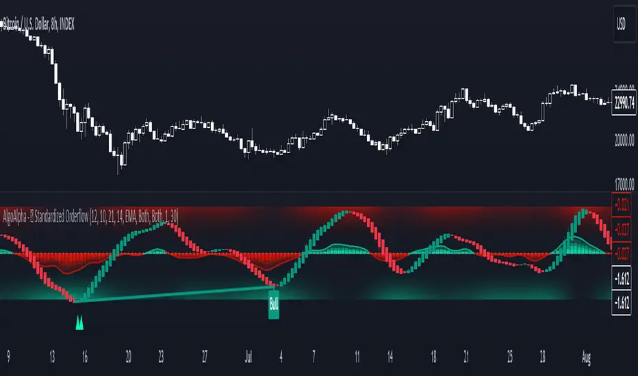
Standardized Orderflow [AlgoAlpha]Introducing the Standardized Orderflow indicator by AlgoAlpha. This innovative tool is designed to enhance your trading strategy by providing a detailed analysis of order flow and velocity. Perfect for traders who seek a deeper insight into market dynamics, it's packed with features that cater to various trading styles. 🚀📊
Key Features:
📈 Order Flow Analysis: At its core, the indicator analyzes order flow, distinguishing between bullish and bearish volume within a specified period. It uses a unique standard deviation calculation for normalization, offering a clear view of market sentiment.
🔄 Smoothing Options: Users can opt for a smoothed representation of order flow, using a Hull Moving Average (HMA) for a more refined analysis.
🌪️ Velocity Tracking: The indicator tracks the velocity of order flow changes, providing insights into the market's momentum.
🎨 Customizable Display: Tailor the display mode to focus on either order flow, order velocity, or both, depending on your analysis needs.
🔔 Alerts for Critical Events: Set up alerts for crucial market events like crossover/crossunder of the zero line and overbought/oversold conditions.
How to Use:
1. Setup: Easily configure the indicator to match your trading strategy with customizable input parameters such as order flow period, smoothing length, and moving average types.
2. Interpretation: Watch for bullish and bearish columns in the order flow chart, utilize the Heiken Ashi RSI candle calculation, and look our for reversal notations for additional market insights.
3. Alerts: Stay informed with real-time alerts for key market events.
Code Explanation:
- Order Flow Calculation:
The core of the indicator is the calculation of order flow, which is the sum of volumes for bullish or bearish price movements. This is followed by normalization using standard deviation.
orderFlow = math.sum(close > close ? volume : (close < close ? -volume : 0), orderFlowWindow)
orderFlow := useSmoothing ? ta.hma(orderFlow, smoothingLength) : orderFlow
stdDev = ta.stdev(orderFlow, 45) * 1
normalizedOrderFlow = orderFlow/(stdDev + stdDev)
- Velocity Calculation:
The velocity of order flow changes is calculated using moving averages, providing a dynamic view of market momentum.
velocityDiff = ma((normalizedOrderFlow - ma(normalizedOrderFlow, velocitySignalLength, maTypeInput)) * 10, velocityCalcLength, maTypeInput)
- Display Options:
Users can choose their preferred display mode, focusing on either order flow, order velocity, or both.
orderFlowDisplayCond = displayMode != "Order Velocity" ? display.all : display.none
wideDisplayCond = displayMode != "Order Flow" ? display.all : display.none
- Reversal Indicators and Divergences:
The indicator also includes plots for potential bullish and bearish reversals, as well as regular and hidden divergences, adding depth to your market analysis.
bullishReversalCond = reversalType == "Order Flow" ? ta.crossover(normalizedOrderFlow, -1.5) : (reversalType == "Order Velocity" ? ta.crossover(velocityDiff, -4) : (ta.crossover(velocityDiff, -4) or ta.crossover(normalizedOrderFlow, -1.5)) )
bearishReversalCond = reversalType == "Order Flow" ? ta.crossunder(normalizedOrderFlow, 1.5) : (reversalType == "Order Velocity" ? ta.crossunder(velocityDiff, 4) : (ta.crossunder(velocityDiff, 4) or ta.crossunder(normalizedOrderFlow, 1.5)) )
In summary, the Standardized Orderflow indicator by AlgoAlpha is a versatile tool for traders aiming to enhance their market analysis. Whether you're focused on short-term momentum or long-term trends, this indicator provides valuable insights into market dynamics. 🌟📉📈
Cast ForwardThis indicator will not forecast price action. It will not predict price movement nor will it in any way predict the outcome of any trade you may take. This is not a signal for buying or selling. You must do your own back testing and analysis for trading.
Time and price are the two most important components of market data. Where was price at what time? To help visualize this question I created this indicator. It allows for the previous session data to be overlayed onto the chart offset forward 24 hours. What this means is that you have the high, (high/low)/2, and low of each candle plotted on top of your chart for the time frame of the current chart, but offset so that the data from the current candle has the data from the corresponding candle 24 hours prior lined up on the x-axis.
SMA Logic: I used the SMA (Simple Moving Average) function with a length of 1 to plot the data points without any smoothing to give the true values of the data.
For Intraday Charting
For Electronic Trading Hours:
In order to line up the data correctly, for intraday charts, I used the current chart timeframe and divided it into 1380 (number of minutes in the 23 hour futures market trading day) to set the data offset. Using the same math logic, this indicator also gives the correct correlated data on the 30 second time frame. If the chart time frame that is currently being used does not allow for correct data correlation (not a factor of 1380) it will not plot the data.
For Regular Trading Hours:
In order to line up the data correctly, for intraday charts, I used the current chart timeframe and divided it into 405 (number of minutes in the 6 hour 45 minutes New York regular session trading day, including the 15 minute settlement time) to set the data offset. This indicator also gives the correct correlated data on the 30 second time frame. If the chart time frame that is currently being used does not allow for correct data correlation (not a factor of 405) it will not plot the data.
For the Daily Chart:
This indicator plots a visualization of the 20-40-60 day IPDA data range; (The IPDA data range helps traders identify liquidity, price gaps, and equilibrium points in the market, providing insights for optimal trade entries and market structure shifts). It does this using the same SMA logic as the intraday plot. What this means is it offsets the historical data of the daily chart 20, 40, or 60 bars forward. You can plot any combination of the three on the chart at one time, but these will not show on the intraday chart. This allows for visualization of where the market will possibly seek liquidity, seek to rebalance, or seek equilibrium in the future.

Live Economic Calendar by toodegrees⚠️ PLEASE READ ⚠️
Although this indicator is accurate in showcasing live and upcoming News Events, checking the original sources is always suggested. This indicator aims to save Time, but due to limitations it may not be 100% correct 100% of the Time.
Description:
The Live Economic Calendar indicator seamlessly integrates with external news sources to provide real-Time, upcoming, and past financial news directly on your Tradingview chart.
By having a clear understanding of when news are planned to be released, as well as their respective impact, analysts can prepare their weeks and days in advance. These injections of volatility can be harnessed by analysts to support their thesis, or may want to be avoided to ensure higher probability market conditions. Fundamentals and news releases transcend the boundaries of technical analysis, as their effects are difficult to predict or estimate.
Designed for both novice and experienced traders, the Live Economic Calendar indicator enhances your analysis by keeping you informed of the latest and upcoming market-moving news.
This is achieved with three different visual components:
News Table: A dedicated News Table shows the Day of the Week, Date, Time of the Day, Currency, Expected Impact, and News Name for each event (in chronological order). Once a news event has occurred, or the day is over, it will be greyed out – helping to focus on the next upcoming news events.
News Lines: Vertical lines plotted in the future help analysts monitor upcoming news events; vertical lines in the past help analysts spot and backtest previous news events that already occurred.
News Labels: Color-coded news labels will plot once the news events have occurred. This not only gives analysts a minimalistic visual cue, but also retains the information of which news were released at that Time in their tooltips.
Forex Factory Calendar News Feed:
The Forex Factory Data Feed includes news events from January 2007 to the present. The data is updated daily. Please see the Technical Description below for more information.
Forex Factory provides news for all major currencies and markets:
Australia (AUD)
Canada (CAD)
Switzerland (CHF)
China (CNY)
European Union (EUR)
United Kingdom (GBP)
Japan (JPY)
New Zealand (NZD)
United States of America (USD)
Further, there are four types of news impact, defined by respective color-coding which is retained to avoid confusion:
⚪ Holiday
🟡 Low Impact
🟠 Medium Impact
🔴 High Impact
News' Time of the day data is in 24H format, and 'All Day' news are marked at Daily candle open.
⚠️ Original Release Notes ⚠️
The original release of this indicator supports the Forex Factory News Calendar in EST (New York Time). Future updates will include multiple news sources, as well as supporting different Timezones.
Given Data limitations, the Daily chart can omit some data due to the market being close on some days. This will be fixed in the future once an efficient solution is implemented.
Key Features:
Impact-Based News Filtering: Filter news items based on their expected impact (holiday, low, medium, high) to focus on the most market-critical information.
Symbol-Specific News: Automatically filter news to display only what's relevant to the currency pair or trading symbol you are analyzing.
Custom Currency News: Want to see more than the news relevant to the current symbol? Toggle which markets' news you are most interested in.
Chart History: Keep your charts clean by displaying only the drawings of Today's news, or This Week's news.
Custom Lookback: Look further back in Time by choosing a custom number of Lookback Days, allowing you to backtest and keep in mind salient news events from the past.
Line and Label Customization: Both the News Lines and Labels are highly customizable (except the colors), allowing you to make the indicator yours.
Table History: Choose whether to focus on Today's news only, or the news for This Week.
Table Customization: The table colors and position are highly customizable, allowing you to make it fit your visual preference and your layouts' aesthetic.
"Wondering how it's done? 👇"
Technical Description:
This script utilizes Pine Seeds , a service integrated with TradingView for importing custom data. This stunning feature enables users to upload and access custom End Of Day (EOD) data, which can be updated as frequently as five times daily.
This data can be imported in one of two formats:
Single Value: integer or float
Candle Data: open, high, low, close, volume
Upon encountering Pine Seeds, I recognized its potential for importing financial news events. Given that Forex Factory is a primary source of financial news in my personal analysis, integrating it into my layouts seemed like an exciting opportunity. This integration is expected to provide significant value to users looking to integrate additional news feeds all in one place.
Development Challenges:
Format Limitations: News events must be converted into numerical values for import, due to the required Pine Seeds format.
Amount of Data: With all currencies considered, the system may encounter over 40 news events in a single day.
Data Availability: The reliance on End Of Day (EOD) data means that information for the current day is displayed with a delay, and accessing future data is not possible.
Solutions:
Encoding: Each news event is encoded as an integer in the "DCHHMMITYP" format.
D = day of the week
C = currency
HHMM = Time of day
I = news impact
TYP = event ID (see Event Library A and Event Library B )
To ensure data assignment for each candle across the open, high, low, close, and volume series, the value "999" is used as a placeholder:
Importing: Utilizing the encoding system, up to five news events per day can be imported for a singular Pine Seeds custom symbol.
By creating multiple custom Pine Seeds Symbols, efficient imports of a larger number of events is then easily achievable. Nine unique symbols have been established, accommodating up to 45 news events per day.
These symbols are searchable, and accessible as " TOODEGREES_FOREX_FACTORY_SLOT_N " where N ranges from 1 to 9.
The Pine Seeds data feed appears as follows:
Uploading Schedule: To ensure analysts are informed about current and upcoming week's news, events are uploaded one week in advance.
This approach is vital for preparing for potential market impacts across various asset classes and currencies, allowing visibility of an entire week's news ahead of Time.
Data Scraping:
Unfortunately Forex Factory doesn't offer an API to fetch their news feed.
Hence an ad hoc python scraper was developed to read and save news events from January 2007 till the present leveraging Selenium. The scraper algorithm is part of a larger script responsible for scraping data, formatting data, and creating all necessary datasets.
The pseudo-code for the python script is as follows:
Read and save news event data on Forex Factory
Format day of the week, currency, Time of the day, and impact data for the Encoding
Encode and save News Event IDs – Event ID dataset is created
Format news data for Pine Seeds (roll-back date by one week, assign news to open, high, low, close, and volume values)
Create Pine Seeds Datasets
This script is ran everyday at Futures market close (16:00 EST) to update the last part of the each dataset, ensuring accuracy, and taking into account last-minute news additions or revisions.
Once the data (next week's news) is imported by the Live Economic Calendar indicator, it's immediately decoded by leveraging the Forex Factory Decoding Library , and saved into an array.
Upon a new week open, the decoded data is used to plot news events on the chart and in the news table.
See the inner workings of these processes in the Forex Factory Utility Library .
Although these libraries are specifically built for this indicator, feel free to use them to create your own scripts. Looking forward to see what the Pine Script community comes up with!
Thank you for making it this far. Enjoy!
Ciao,
toodegrees
This tool is available ONLY on the TradingView platform.
Terms and Conditions
Our charting tools are provided for informational and educational purposes only and do not constitute financial, investment, or trading advice. Our charting tools are not designed to predict market movements or provide specific recommendations. Users should be aware that past performance is not indicative of future results and should not be relied upon for making financial decisions. By using our charting tools, the user agrees that Toodegrees and the Toodegrees Team are not responsible for any decisions made based on the information provided by these charting tools. The user assumes full responsibility and liability for any actions taken and the consequences thereof, including any loss of money or investments that may occur as a result of using these products. Hence, by using these charting tools, the user accepts and acknowledges that Toodegrees and the Toodegrees Team are not liable nor responsible for any unwanted outcome that arises from the development, or the use of these charting tools. Finally, the user indemnifies Toodegrees and the Toodegrees Team from any and all liability.
By continuing to use these charting tools, the user acknowledges and agrees to the Terms and Conditions outlined in this legal disclaimer.

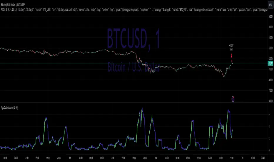
AlgoDude_Volume1. Timeframe Selection (selectedTimeframe):
Allows the user to choose the timeframe for the volume data analysis.
Options range from 1 minute to 1 month, including 1, 3, 5, 15, 30, 45 minutes, 1, 2, 3, 4 hours, and daily, weekly, monthly.
2.Moving Average Length (maLength):
Users can specify the length of the moving average applied to the inverse volume.
The range for this input is from 1 to 200 periods, with a default value of 14.
These inputs provide flexibility in analyzing volume data over various timeframes and smoothing the inverse volume data with a moving average of chosen length.
Zemog Channels[Zemogtrading]Channels Strategy
User Description:
This Channels strategy is a powerful technical analysis tool that empowers traders with a comprehensive view of the market's support and resistance levels. Designed for both beginners and experienced traders, this strategy brings a systematic and adaptable approach to chart analysis.
Default Parameters:
Swing Length (SL): 45
Higher Timeframe: Daily (D)
Multiplier for Level 2: 3.5
Multiplier for Level 3: 12
How It Works:
Swing Analysis: The Swing Length (SL) parameter allows users to fine-tune the sensitivity of the strategy. A higher SL value provides a more smoothed-out analysis, ideal for a broader market perspective, while a lower value enhances responsiveness to short-term price movements.
Higher Timeframe Insights: The Channels fetches high and low prices from a user-specified higher timeframe (default: Daily). This ensures that the strategy is well-informed by significant price levels from a broader market context.
Dynamic ATR Calculation: The Average True Range (ATR) adapts dynamically to changing market conditions. This ensures that support and resistance levels adjust in real-time based on the prevailing volatility, providing traders with adaptive insights.
Smoothed Support and Resistance: Utilizing a Smoothed Moving Average (SMA), the strategy calculates support and resistance levels based on high and low prices from the higher timeframe. This smoothing effect enhances clarity in identifying key levels, facilitating more informed trading decisions.
Additional Levels: The Channels introduces Level 2 and Level 3 support and resistance zones. Users can customize multipliers for these levels, allowing for the identification of secondary zones for potential market reversals.
Visualization: The strategy vividly plots support and resistance levels on the chart. Green lines indicate support, red lines denote resistance, and yellow lines represent additional support at Level 3.
Using Channels is a versatile tool that equips traders with a deeper understanding of crucial market levels. By seamlessly integrating swing analysis, higher timeframe data, and adaptive calculations, this strategy offers a holistic and user-friendly approach to technical analysis.

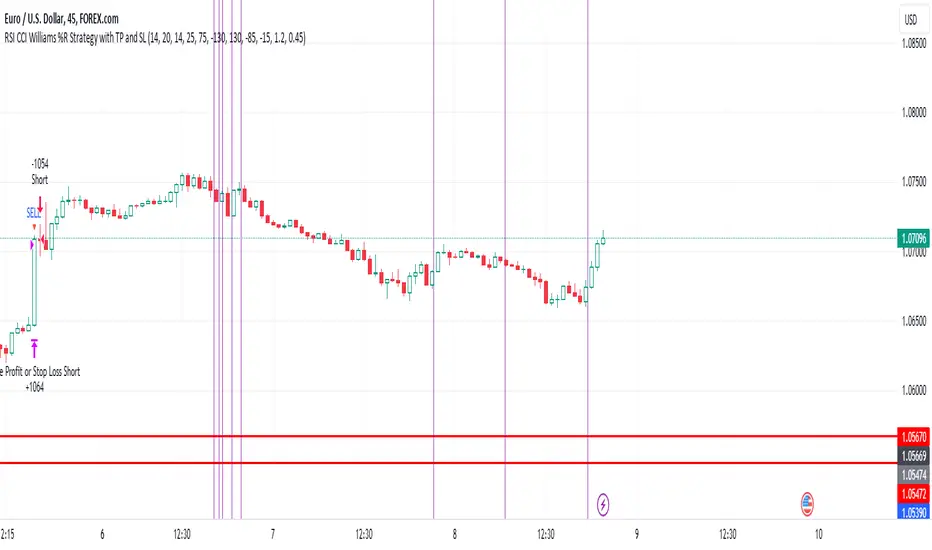
EUR/USD 45 MIN Strategy - FinexBOTThis strategy uses three indicators:
RSI (Relative Strength Index) - It indicates if a stock is potentially overbought or oversold.
CCI (Commodity Channel Index) - It measures the current price level relative to an average price level over a certain period of time.
Williams %R - It is a momentum indicator that shows whether a stock is at the high or low end of its trading range.
Long (Buy) Trades Open:
When all three indicators suggest that the stock is oversold (RSI is below 25, CCI is below -130, and Williams %R is below -85), the strategy will open a buy position, assuming there is no current open trade.
Short (Sell) Trades Open:
When all three indicators suggest the stock is overbought (RSI is above 75, CCI is above 130, and Williams %R is above -15), the strategy will open a sell position, assuming there is no current open trade.
SL (Stop Loss) and TP (Take Profit):
SL (Stop Loss) is 0.45%.
TP (Take Profit) is 1.2%.
The strategy automatically sets these exit points as a percentage of the entry price for both long and short positions to manage risks and secure profits. You can easily adopt these inputs according to your strategy. However, default settings are recommended.
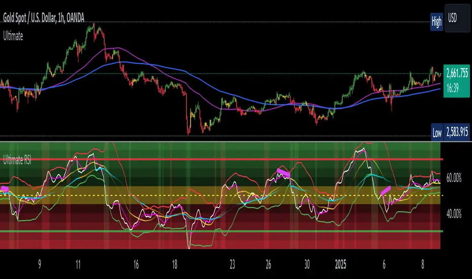
Ultimate RSIThis indicator is a customized version of the RSI indicator that by default utilizes Bollinger Bands. It have included two layers of bands, with separate standard deviations. The indicator is fully customizable.
The indicator displays bullish and bearish divergence from price.
You are able to change the moving average that is used to calculate both the RSI itself, as well as the moving average used for the Bollinger Bands.
I have included fills that color the background to indicate various zones of RSI values.
Price tends to either reject or move quickly at these levels.
I have a yellow RSI zone that indicates a sideways market with little to no momentum with default values of 45 to 55. These are areas where trading is stagnant and you should likely avoid placing trades.
There is now an ATR feature to adjust the Bollinger Bands with ATR (Average True Range).
In order to trade with this indicator, you should watch for the white line (RSI) to cross into the Bollinger Bands, then cross over the yellow moving average (Basis line), where you would enter a BUY or SELL.
Watch this indicator in action and look for patterns. Draw vertical lines on the chart where you would have wanted to buy or sell and study this to understand how to make better trading decisions.
NOTE:
While not required in order to use this indicator, it was designed to visually work with another indicator of mine called The Ultimate Buy and Sell Indicator. I recommend using both together as they are a strong pair of indicators that share the same settings. This indicator while it can be used independently can also help you visualize the settings changes made to the other one which are unable to be displayed on the main chart by that indicator.
Open-Close Difference Signalopen close signal This code will plot an upward triangle shape at the low of the candle when either the difference between open and close or the difference between close and open is above 45 points. This can be considered a buy signal. Adjust the threshold value as needed using the script's settings on TradingView.

RSI Custom LevelsRSI Custom Levels is a "one stop shop" for a complete strategy based on RSI.
AS per principal: RSI oscillates between 0-100 and therefore the indicator is build around various parameters of RSI. It comprises of 4 different levels of RSI and therefore highlights the candles accordingly.
Understanding each LEVEL:
Level 1 (Highlight): Highlights candles that have an RSI value (closing basis) less than Level 1 specified value (default 20)
Level 2 (Highlight): Highlights candles that have an RSI value (closing basis) greater than Level 1 specified value (default 20) and less than Level 2 specified value (default 45)
Level 4 (Highlight): Highlights candles that have an RSI value (closing basis) greater than Level 4 specified value (default 80)
Level 3 (Highlight): Highlights candles that have an RSI value (closing basis) greater than Level 3 specified value (default 55) and less than Level 4 specified value (default 80)
The most efficient way to trade is as follows:
TRENDING SETUPS:
Uptrend Setups: When RSI enters Level 3 with exit at Level 4
Downtrend Setups: When RSI enters Level 2 with exit at Level 1
SIDEWAYS APPLICATION:
When RSI is in between Level 2 and 3 that area has no highlights as the system considers it to be FLAT and non oscillating.
OVERSTRETCHED APPLICATIONS:
Downtrend Reversal: When RSI enters Level 2 from Level 1 that is a sign for a downtrend reversal.
Uptrend Reversal: When RSI enters Level 3 from Level 2 that is a sign for a uptrend reversal.
Moreover the most ideal scenario is to convert the colour of all candles into white (in dark theme) or black(in light theme) for best performance.
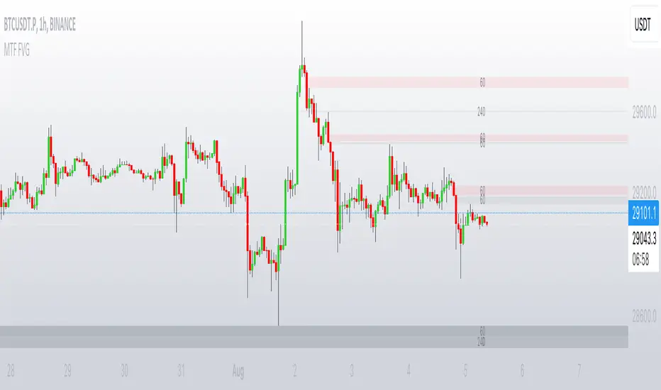
MTF FVGThis script finds Imbalance (Fair Value Gap (FVG)) on multi timeframes.
If needed all TF can be used at once: 1, 3, 5, 15, 30, 45, 60, 120, 180, 240, D, W.
It finds FVG on any desired TF that is greater or equal than TF on the chart.
FVG stands for fair value gap, which is a three-candle structure that indicates an imbalance or inefficiency in the market. An imbalance means that the buying and selling is not equal, and there is a gap between the fair value and the market value of an asset. A bullish FVG shows that the market value is lower than the fair value, and a bearish FVG shows the opposite.
FVG takes place in a series of 3 candles when the middle candle gaps up or down. This signals strong buying or selling pressure in the direction of the gap. When a gap occurs the wicks of the candles do not overlap each other.
ICT Macros [LuxAlgo]The ICT Macros indicator aims to highlight & classify ICT Macros, which are time intervals where algorithmic trading takes place to interact with existing liquidity or to create new liquidity.
🔶 SETTINGS
🔹 Macros
Macro Time options (such as '09:50 AM 10:10'): Enable specific macro display.
Top Line , Mid Line , Bottom Line and Extending Lines options: Controls the lines for the specific macro.
🔹 Macro Classification
Length : A length to detect Market Structure Brakes and classify macro type based on detection.
Swing Area : Swing or Liquidity Area selection, highest/lowest of the wick or the candle bodies.
Accumulation , Manipulation and Expansion color options for the classified macros.
🔹 Others
Macro Texts : Controls both the size and the visibility of the macro text.
Alert Macro Times in Advance (Minutes) : This option will plot a vertical line presenting the start of the next macro time. The line will not appear all the time, but it will be there based on remaining minutes specified in the option.
Daylight Saving Time (DST) : Adjust time appropriate to Daylight Saving Time of the specific region.
🔶 USAGE
A macro is a way to automate a task or procedure which you perform on a regular basis.
In the context of ICT's teachings, a macro is a small program or set of instructions that unfolds within an algorithm, which influences price movements in the market. These macros operate at specific times and can be related to price runs from one level to another or certain market behaviors during specific time intervals. They help traders anticipate market movements and potential setups during specific time intervals.
To trade these effectively, it is important to understand the time of day when certain macros come into play, and it is strongly advised to introduce the concept of liquidity in your analysis.
Macros can be classified into three categories where the Macro classification is calculated based on the Market Structure prior to macro and the Market Structure during the macro duration:
Manipulation Macro
Manipulation macros are characterized by liquidity being swept both on the buyside and sellside.
Expansion Macro
Expansion macros are characterized by liquidity being swept only on the buyside or sellside. Prices within these macros are highly correlated with the overall trend.
Accumulation Macro
Accumulation macros are characterized by an accumulation of liquidity. Prices within these macros tend to range.
The script returns the maximum/minimum price values reached during the macro interval alongside the average between the maximum/minimum and extends them until a new macro starts. These levels can act as supports and resistances.
🔶 DETAILS
All required data for the macro detection and classification is retrieved using 1 minute data sets, this includes candles as well as pivot/swing highs and lows. This approach guarantees the visually presented objects are same (same highs/lows) on higher timeframes as well as the macro classification remain same as it is in 1 min charts.
8 Macros can be displayed by the script (4 are enabled by default):
02:33 AM 03:00 London Macro
04:03 AM 04:30 London Macro
08:50 AM 09:10 New York Macro
09:50 AM 10:10 New York Macro
10:50 AM 11:10 New York Macro
11:50 AM 12:10 New York Launch Macro
13:10 PM 13:40 New York Macro
15:15 PM 15:45 New York Macro
🔶 ALERTS
When an alert is configured, the user will have the ability to be notified in advance of the next Macro time, where the value specified in 'Alert Macro Times in Advance (Minutes)' option indicates how early to be notified.
🔶 LIMITATIONS
The script is supported on 1 min, 3 mins and 5 mins charts.
🔶 RELATED SCRIPTS