Ripple (XRP) Model PriceAn article titled Bitcoin Stock-to-Flow Model was published in March 2019 by "PlanB" with mathematical model used to calculate Bitcoin model price during the time. We know that Ripple has a strong correlation with Bitcoin. But does this correlation have a definite rule?
In this study, we examine the relationship between bitcoin's stock-to-flow ratio and the ripple(XRP) price.
The Halving and the stock-to-flow ratio
Stock-to-flow is defined as a relationship between production and current stock that is out there.
SF = stock / flow
The term "halving" as it relates to Bitcoin has to do with how many Bitcoin tokens are found in a newly created block. Back in 2009, when Bitcoin launched, each block contained 50 BTC, but this amount was set to be reduced by 50% every 210,000 blocks (about 4 years). Today, there have been three halving events, and a block now only contains 6.25 BTC. When the next halving occurs, a block will only contain 3.125 BTC. Halving events will continue until the reward for minors reaches 0 BTC.
With each halving, the stock-to-flow ratio increased and Bitcoin experienced a huge bull market that absolutely crushed its previous all-time high. But what exactly does this affect the price of Ripple?
Price Model
I have used Bitcoin's stock-to-flow ratio and Ripple's price data from April 1, 2014 to November 3, 2021 (Daily Close-Price) as the statistical population.
Then I used linear regression to determine the relationship between the natural logarithm of the Ripple price and the natural logarithm of the Bitcoin's stock-to-flow (BSF).
You can see the results in the image below:
Basic Equation : ln(Model Price) = 3.2977 * ln(BSF) - 12.13
The high R-Squared value (R2 = 0.83) indicates a large positive linear association.
Then I "winsorized" the statistical data to limit extreme values to reduce the effect of possibly spurious outliers (This process affected less than 4.5% of the total price data).
ln(Model Price) = 3.3297 * ln(BSF) - 12.214
If we raise the both sides of the equation to the power of e, we will have:
============================================
Final Equation:
■ Model Price = Exp(- 12.214) * BSF ^ 3.3297
Where BSF is Bitcoin's stock-to-flow
============================================
If we put current Bitcoin's stock-to-flow value (54.2) into this equation we get value of 2.95USD. This is the price which is indicated by the model.
There is a power law relationship between the market price and Bitcoin's stock-to-flow (BSF). Power laws are interesting because they reveal an underlying regularity in the properties of seemingly random complex systems.
I plotted XRP model price (black) over time on the chart.
Estimating the range of price movements
I also used several bands to estimate the range of price movements and used the residual standard deviation to determine the equation for those bands.
Residual STDEV = 0.82188
ln(First-Upper-Band) = 3.3297 * ln(BSF) - 12.214 + Residual STDEV =>
ln(First-Upper-Band) = 3.3297 * ln(BSF) – 11.392 =>
■ First-Upper-Band = Exp(-11.392) * BSF ^ 3.3297
In the same way:
■ First-Lower-Band = Exp(-13.036) * BSF ^ 3.3297
I also used twice the residual standard deviation to define two extra bands:
■ Second-Upper-Band = Exp(-10.570) * BSF ^ 3.3297
■ Second-Lower-Band = Exp(-13.858) * BSF ^ 3.3297
These bands can be used to determine overbought and oversold levels.
Estimating of the future price movements
Because we know that every four years the stock-to-flow ratio, or current circulation relative to new supply, doubles, this metric can be plotted into the future.
At the time of the next halving event, Bitcoins will be produced at a rate of 450 BTC / day. There will be around 19,900,000 coins in circulation by August 2025
It is estimated that during first year of Bitcoin (2009) Satoshi Nakamoto (Bitcoin creator) mined around 1 million Bitcoins and did not move them until today. It can be debated if those coins might be lost or Satoshi is just waiting still to sell them but the fact is that they are not moving at all ever since. We simply decrease stock amount for 1 million BTC so stock to flow value would be:
BSF = (19,900,000 – 1.000.000) / (450 * 365) =115.07
Thus, Bitcoin's stock-to-flow will increase to around 115 until AUG 2025. If we put this number in the equation:
Model Price = Exp(- 12.214) * 114 ^ 3.3297 = 36.06$
Ripple has a fixed supply rate. In AUG 2025, the total number of coins in circulation will be about 56,000,000,000. According to the equation, Ripple's market cap will reach $2 trillion.
Note that these studies have been conducted only to better understand price movements and are not a financial advice.
Cerca negli script per "环保行业指数2025年6月4日走势预测"

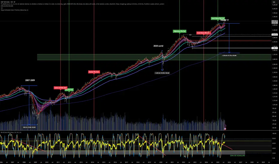
Major & Modern Wars TimelineDescription:
This indicator overlays vertical lines and labels on your chart to mark the start and end dates of major global wars and modern conflicts.
Features:
Displays start (red line + label) and end (green line + label) for each war.
Covers 20th century wars (World War I, World War II, Korean War, Vietnam War, Gulf War, Afghanistan, Iraq).
Includes modern conflicts: Syrian Civil War, Ukraine War, and Israel–Hamas War.
For ongoing conflicts, the end date is set to 2025 for timeline visualization.
Customizable: label position (above/below bar), line width.
Works on any chart timeframe, overlaying events on financial data.
Use case:
Useful for historical market analysis (e.g., gold, oil, S&P 500), helping traders and researchers see how wars and conflicts align with market movements.
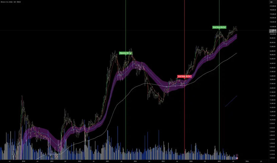
Sorry Cryptoface Market Cypher B//@version=5
indicator("Sorry Cryptoface Market Cypher B", shorttitle="SorryCF B", overlay=false)
// 🙏 Respect to Cryptoface
// Market Cipher is the brainchild of Cryptoface, who popularized the
// combination of WaveTrend, Money Flow, RSI, and divergence signals into a
// single package that has helped thousands of traders visualize momentum.
// This script is *not* affiliated with or endorsed by him — it’s just an
// open-source educational re-implementation inspired by his ideas.
// Whether you love him or not, Cryptoface deserves credit for taking complex
// oscillator theory and making it accessible to everyday traders.
// -----------------------------------------------------------------------------
// Sorry Cryptoface Market Cypher B
//
// ✦ What it is
// A de-cluttered, optimized rework of the popular Market Cipher B concept.
// This fork strips out repaint-prone code and redundant signals, adds
// higher-timeframe and trend filters, and introduces volatility &
// money-flow gating to cut down on the "confetti signals" problem.
//
// ✦ Key Changes vs. Original MC-B
// - Non-repainting security(): switched to request.security(..., lookahead_off)
// - Inputs updated to Pine v5 (input.int, input.float, etc.)
// - Trend filter: EMA or HTF WaveTrend required for alignment
// - Volatility filter: minimum ADX & ATR % threshold to avoid chop
// - Money Flow filter: signals require minimum |MFI| magnitude
// - WaveTrend slope check: reject flat or contra-slope crosses
// - Cooldown filter: prevents multiple signals within N bars
// - Bar close confirmation: dots/alerts only fire once a candle is closed
// - Hidden divergences + “second range” divergences disabled by default
// (to reduce noise) but can be toggled on
//
// ✦ Components
// - WaveTrend oscillator (2-line system + VWAP line)
// - Money Flow Index + RSI overlay
// - Stochastic RSI
// - Divergence detection (WT, RSI, Stoch)
// - Optional Schaff Trend Cycle
// - Optional Sommi flags/diamonds (HTF confluence markers)
//
// ✦ Benefits
// - Fewer false positives in sideways markets
// - Signals aligned with trend & volatility regimes
// - Removes repaint artifacts from higher-timeframe sources
// - Cleaner chart (reduced “dot spam”)
// - Still flexible: all original toggles/visuals retained
//
// ✦ Notes
// - This is NOT the official Market Cipher.
// - Educational / experimental use only. Do your own testing.
// - Best tested on 2H–4H timeframes; short TFs may still look choppy
//
// ✦ Credits
// Original open-source inspirations by LazyBear, RicardoSantos, LucemAnb,
// falconCoin, dynausmaux, andreholanda73, TradingView community.
// This fork modified by Lumina+Thomas (2025).
// -----------------------------------------------------------------------------
MATEOANUBISANTIDear traders, investors, and market enthusiasts,
We are excited to share our High-Low Indicator Range for on . This report aims to provide a clear and precise overview of the highest and lowest values recorded by during this specific hour, equipping our community with a valuable tool for making informed and strategic market decisions.

MATEOANUBISANTI-BILLIONSQUATDear traders, investors, and market enthusiasts,
We are excited to share our High-Low Indicator Range for on . This report aims to provide a clear and precise overview of the highest and lowest values recorded by during this specific hour, equipping our community with a valuable tool for making informed and strategic market decisions.

AmazingGPT//@version=6
indicator("AmazingGPT", shorttitle="AmazingGPT", overlay=true, max_lines_count=500, max_labels_count=500)
// ─────────────────────────── Inputs
group_ma = "SMMA"
group_avwap = "AVWAP"
group_fibo = "Fibo"
group_toler = "Yakınlık (2/3)"
group_trig = "Trigger & Onay"
group_misc = "Görsel/HUD"
// SMMA
len21 = input.int(21, "SMMA 21", group=group_ma, minval=1)
len50 = input.int(50, "SMMA 50", group=group_ma, minval=1)
len200 = input.int(200, "SMMA 200", group=group_ma, minval=1)
// AVWAP
const int anchorDefault = timestamp("2025-06-13T00:00:00")
anchorTime = input.time(anchorDefault, "AVWAP Anchor (tarih)", group=group_avwap)
bandMode = input.string("ATR", "Band mode", options= , group=group_avwap)
band1K = input.float(1.0, "Band 1 (×Unit)", step=0.1, group=group_avwap)
band2K = input.float(0.0, "Band 2 (×Unit)", step=0.1, group=group_avwap)
// Fibo
useAutoFib = input.bool(false, "Auto Fib (son 252 bar HL)", group=group_fibo)
fibL_in = input.float(0.0, "Swing Low (fiyat)", group=group_fibo, step=0.01)
fibH_in = input.float(0.0, "Swing High (fiyat)", group=group_fibo, step=0.01)
// Yakınlık (2/3) – ayrı eşikler
tolMA = input.float(1.00, "Yakınlık eşiği – SMMA (×ATR)", minval=0.0, step=0.05, group=group_toler)
tolAV = input.float(0.80, "Yakınlık eşiği – AVWAP (×ATR)", minval=0.0, step=0.05, group=group_toler)
tolFibo = input.float(0.60, "Yakınlık eşiği – Fibo (×ATR)", minval=0.0, step=0.05, group=group_toler)
starterTolMA = input.float(1.00, "Starter SMMA eşiği (×ATR)", minval=0.0, step=0.05, group=group_toler)
// Trigger & Onay
useDailyLock = input.bool(true, "Lock core calcs to Daily (1D)", group=group_trig)
triggerSrc = input.string("Auto", "Trigger Source", options= , group=group_trig)
useCH3auto = input.bool(true, "Auto: CH3 fallback ON", group=group_trig)
fallbackBars = input.int(3, "Fallback after N bars", minval=1, group=group_trig)
tamponTL = input.float(0.10, "Tampon (TL)", step=0.01, group=group_trig)
tamponATRf = input.float(0.15, "Tampon (×ATR)", step=0.01, group=group_trig)
capATR = input.float(0.60, "Cap (kovalama) ≤ ×ATR", step=0.05, group=group_trig)
vetoATR = input.float(1.00, "Veto (asla kovala) ≥ ×ATR", step=0.05, group=group_trig)
useRSIbreak = input.bool(false, "RSI≥50 (sadece kırılımda)", group=group_trig)
nearCloseStarter = input.bool(true, "Starter (reclaim gününde) ENABLE", group=group_trig)
// Görsel
showHud = input.bool(true, "HUD göster", group=group_misc)
showBands = input.bool(true, "AVWAP bantlarını göster", group=group_misc)
// ─────────────────────────── Daily sources (lock)
smma21D = request.security(syminfo.tickerid, "D", ta.rma(close, len21))
smma50D = request.security(syminfo.tickerid, "D", ta.rma(close, len50))
smma200D = request.security(syminfo.tickerid, "D", ta.rma(close, len200))
atrD = request.security(syminfo.tickerid, "D", ta.atr(14))
rsiD = request.security(syminfo.tickerid, "D", ta.rsi(close, 14))
v20D = request.security(syminfo.tickerid, "D", ta.sma(volume, 20))
dHighD = request.security(syminfo.tickerid, "D", high)
h3HighD = request.security(syminfo.tickerid, "D", ta.highest(high, 3))
ch3CloseD= request.security(syminfo.tickerid, "D", ta.highest(close, 3))
// ─────────────────────────── Core calcs (lock uygulanmış)
smma21 = useDailyLock ? smma21D : ta.rma(close, len21)
smma50 = useDailyLock ? smma50D : ta.rma(close, len50)
smma200 = useDailyLock ? smma200D : ta.rma(close, len200)
atr = useDailyLock ? atrD : ta.atr(14)
rsi = useDailyLock ? rsiD : ta.rsi(close, 14)
v20 = useDailyLock ? v20D : ta.sma(volume, 20)
// ─────────────────────────── AVWAP (anchor sonrası)
tp = hlc3
isAfter = time >= anchorTime
var float cumV = na
var float cumTPV = na
var float cumTP2V = na
if isAfter
cumV := nz(cumV ) + volume
cumTPV := nz(cumTPV ) + tp * volume
cumTP2V := nz(cumTP2V ) + (tp*tp) * volume
else
cumV := na
cumTPV := na
cumTP2V := na
avwap = isAfter ? (cumTPV / cumV) : na
// Band birimi: ATR veya VWAP-σ
vwVar = isAfter ? math.max(0.0, cumTP2V/cumV - avwap*avwap) : na
vwStd = isAfter ? math.sqrt(vwVar) : na
bandUnit = bandMode == "ATR" ? atr : nz(vwStd, 0)
upper1 = isAfter and showBands ? avwap + band1K*bandUnit : na
lower1 = isAfter and showBands ? avwap - band1K*bandUnit : na
upper2 = isAfter and showBands and band2K>0 ? avwap + band2K*bandUnit : na
lower2 = isAfter and showBands and band2K>0 ? avwap - band2K*bandUnit : na
// ─────────────────────────── Fibo (manuel/auto)
var float swingL = na
var float swingH = na
if useAutoFib
swingL := ta.lowest(low, 252)
swingH := ta.highest(high, 252)
else
swingL := fibL_in
swingH := fibH_in
float L = na(swingL) or na(swingH) ? na : math.min(swingL, swingH)
float H = na(swingL) or na(swingH) ? na : math.max(swingL, swingH)
fib382 = na(L) ? na : H - 0.382 * (H - L)
fib500 = na(L) ? na : H - 0.500 * (H - L)
fib618 = na(L) ? na : H - 0.618 * (H - L)
// ─────────────────────────── 2/3 yakınlık (ayrı eşikler)
d21ATR = math.abs(close - smma21) / atr
dAVATR = na(avwap) ? 10e6 : math.abs(close - avwap) / atr
dFATR = na(fib382) ? 10e6 : math.min(math.abs(close - fib382), math.min(math.abs(close - fib500), math.abs(close - fib618))) / atr
near21 = d21ATR <= tolMA
nearAV = dAVATR <= tolAV
nearFib = dFATR <= tolFibo
countConfluence = (near21?1:0) + (nearAV?1:0) + (nearFib?1:0)
twoOfThree = countConfluence >= 2
// ─────────────────────────── Trigger (Auto → CH3 fallback)
d1High = useDailyLock ? dHighD : high
h3High = useDailyLock ? h3HighD : ta.highest(high, 3)
ch3Close = useDailyLock ? ch3CloseD : ta.highest(close, 3)
stretch = d21ATR
grindCond = close > smma21 and close > avwap and close > smma21 and close > avwap and close > smma21 and close > avwap and stretch <= 0.6
reclaimCond = (close >= smma21) and (close >= avwap) and twoOfThree
tampon = math.max(tamponTL, tamponATRf*atr)
manualHigh =
triggerSrc == "D-1 High" ? d1High :
triggerSrc == "H3 High" ? h3High : na
manualTrig = not na(manualHigh) ? math.ceil((manualHigh + tampon)/syminfo.mintick)*syminfo.mintick :
triggerSrc == "CH3 Close" ? math.ceil((ch3Close + tampon)/syminfo.mintick)*syminfo.mintick : na
baseHighAuto = grindCond ? h3High : d1High
brokeHigh = high > baseHighAuto
barsNoBreak = ta.barssince(brokeHigh)
useCH3 = useCH3auto and reclaimCond and (barsNoBreak >= fallbackBars)
autoTrig = useCH3 ? math.ceil((ch3Close + tampon)/syminfo.mintick)*syminfo.mintick
: math.ceil((baseHighAuto + tampon)/syminfo.mintick)*syminfo.mintick
trigger = triggerSrc == "Auto" ? autoTrig : manualTrig
// Mesafe filtreleri (cap/veto) ve RSI kırılım filtresi
dist = close - trigger
okCap = dist <= capATR*atr
veto = dist >= vetoATR*atr
rsiOK = not useRSIbreak or (rsi >= 50)
// Starter (sadece reclaim gününde, cap'e değil SMMA yakınlığına bakar)
starterToday = nearCloseStarter and reclaimCond and (d21ATR <= starterTolMA) and (volume >= v20*1.0)
// ─────────────────────────── Plots
plot(smma21, "SMMA21", color=color.new(color.white, 0), linewidth=2)
plot(smma50, "SMMA50", color=color.new(color.blue, 0), linewidth=2)
plot(smma200, "SMMA200", color=color.new(color.red, 0), linewidth=2)
plot(avwap, "AVWAP", color=color.new(color.orange, 0), linewidth=2)
pU1 = plot(upper1, "AVWAP Band1+", color=color.new(color.lime, 40))
pL1 = plot(lower1, "AVWAP Band1-", color=color.new(color.lime, 40))
pU2 = plot(upper2, "AVWAP Band2+", color=color.new(color.green, 70))
pL2 = plot(lower2, "AVWAP Band2-", color=color.new(color.green, 70))
trigColor = okCap ? color.teal : (veto ? color.red : color.gray)
plot(trigger, "Trigger", color=color.new(trigColor, 0), style=plot.style_circles, linewidth=2)
// İşaretler
plotshape(starterToday, title="Starter", style=shape.triangleup, location=location.belowbar, color=color.new(color.teal, 0), size=size.tiny, text="Starter")
breakoutNow = (close >= trigger) and okCap and rsiOK
plotshape(breakoutNow, title="Breakout", style=shape.triangledown, location=location.abovebar, color=color.new(color.fuchsia, 0), size=size.tiny, text="BRK")
// ─────────────────────────── Alerts
alertcondition(starterToday, title="Starter_Ready", message="Starter: reclaim + Δ21 ≤ starterTolMA + v≥v20")
alertcondition(breakoutNow, title="Trigger_Breakout", message="Trigger üstü kapanış (cap OK, RSI filtresi OK)")
// ─────────────────────────── HUD
var label hudLbl = na
if barstate.islast and showHud
hudTxt = "2/3:" + (twoOfThree ? "✅" : "❌") +
" Trg:" + str.tostring(trigger, format.mintick) +
" ATR:" + str.tostring(atr, format.mintick) +
" Δ21:" + str.tostring(d21ATR, "#.##") + "≤" + str.tostring(tolMA, "#.##") +
" ΔAV:" + str.tostring(dAVATR, "#.##") + "≤" + str.tostring(tolAV, "#.##") +
" ΔF:" + str.tostring(dFATR, "#.##") + "≤" + str.tostring(tolFibo, "#.##") +
" RSI50:" + (rsiOK ? "✅" : "❌") +
" Cap:" + (okCap ? "≤"+str.tostring(capATR, "#.##")+" OK" : (veto ? "≥"+str.tostring(vetoATR, "#.##")+" VETO" : ">"+str.tostring(capATR, "#.##")+" FAR"))
if not na(hudLbl)
label.delete(hudLbl)
hudLbl := label.new(bar_index, high, hudTxt, style=label.style_label_upper_left, textcolor=color.white, color=color.new(color.black, 60))

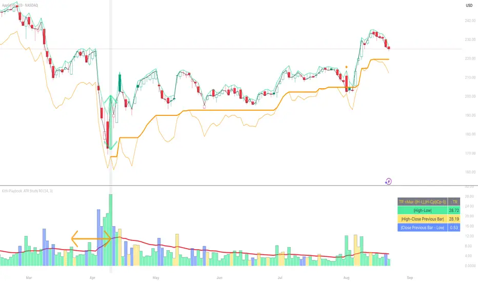
Kitti-Playbook ATR Study R0
Date : Aug 22 2025
Kitti-Playbook ATR Study R0
This is used to study the operation of the ATR Trailing Stop on the Long side, starting from the calculation of True Range.
1) Studying True Range Calculation
1.1) Specify the Bar graph you want to analyze for True Range.
Enable "Show Selected Price Bar" to locate the desired bar.
1.2) Enable/disable "Display True Range" in the Settings.
True Range is calculated as:
TR = Max (|H - L|, |H - Cp|, |Cp - L|)
• Show True Range:
Each color on the bar represents the maximum range value selected:
◦ |H - L| = Green
◦ |H - Cp| = Yellow
◦ |Cp - L| = Blue
• Show True Range on Selected Price Bar:
An arrow points to the range, and its color represents the maximum value chosen:
◦ |H - L| = Green
◦ |H - Cp| = Yellow
◦ |Cp - L| = Blue
• Show True Range Information Table:
Displays the actual values of |H - L|, |H - Cp|, and |Cp - L| from the selected bar.
2) Studying Average True Range (ATR)
2.1) Set the ATR Length in Settings.
Default value: ATR Length = 14
2.2) Enable/disable "Display Average True Range (RMA)" in Settings:
• Show ATR
• Show ATR Length from Selected Price Bar
(An arrow will point backward equal to the ATR Length)
3) Studying ATR Trailing
3.1) Set the ATR Multiplier in Settings.
Default value: ATR Multiply = 3
3.2) Enable/disable "Display ATR Trailing" in Settings:
• Show High Line
• Show ATR Bands
• Show ATR Trailing
4) Studying ATR Trailing Exit
(Occurs when the Close price crosses below the ATR Trailing line)
Enable/disable "Display ATR Trailing" in Settings:
• Show Close Line
• Show Exit Points
(Exit points are marked by an orange diamond symbol above the price bar)
44 MA Near & Green Candle ScannerStocks that have closed just about 44 MA on 14th Aug 2025 and are forming green candles now

Prime NumbersPrime Numbers highlights prime numbers (no surprise there 😅), tokens and the recent "active" feature in "input".
🔸 CONCEPTS
🔹 What are Prime Numbers?
A prime number (or a prime) is a natural number greater than 1 that is not a product of two smaller natural numbers.
Wikipedia: Prime number
🔹 Prime Factorization
The fundamental theorem of arithmetic states that every integer larger than 1 can be written as a product of one or more primes. More strongly, this product is unique in the sense that any two prime factorizations of the same number will have the same number of copies of the same primes, although their ordering may differ. So, although there are many different ways of finding a factorization using an integer factorization algorithm, they all must produce the same result. Primes can thus be considered the "basic building blocks" of the natural numbers.
Wikipedia: Fundamental theorem of arithmetic
Math Is Fun: Prime Factorization
We divide a given number by Prime Numbers until only Primes remain.
Example:
24 / 2 = 12 | 24 / 3 = 8
12 / 3 = 4 | 8 / 2 = 4
4 / 2 = 2 | 4 / 2 = 2
|
24 = 2 x 3 x 2 | 24 = 3 x 2 x 2
or | or
24 = 2² x 3 | 24 = 2² x 3
In other words, every natural/integer number above 1 has a unique representation as a product of prime numbers, no matter how the number is divided. Only the order can change, but the factors (the basic elements) are always the same.
🔸 USAGE
The Prime Numbers publication contains two use cases:
Prime Factorization: performed on "close" prices, or a manual chosen number.
List Prime Numbers: shows a list of Prime Numbers.
The other two options are discussed in the DETAILS chapter:
Prime Factorization Without Arrays
Find Prime Numbers
🔹 Prime Factorization
Users can choose to perform Prime Factorization on close prices or a manually given number.
❗️ Note that this option only applies to close prices above 1, which are also rounded since Prime Factorization can only be performed on natural (integer) numbers above 1.
In the image below, the left example shows Prime Factorization performed on each close price for the latest 50 bars (which is set with "Run script only on 'Last x Bars'" -> 50).
The right example shows Prime Factorization performed on a manually given number, in this case "1,340,011". This is done only on the last bar.
When the "Source" option "close price" is chosen, one can toggle "Also current price", where both the historical and the latest current price are factored. If disabled, only historical prices are factored.
Note that, depending on the chosen options, only applicable settings are available, due to a recent feature, namely the parameter "active" in settings.
Setting the "Source" option to "Manual - Limited" will factorize any given number between 1 and 1,340,011, the latter being the highest value in the available arrays with primes.
Setting to "Manual - Not Limited" enables the user to enter a higher number. If all factors of the manual entered number are in the 1 - 1,340,011 range, these factors will be shown; however, if a factor is higher than 1,340,011, the calculation will stop, after which a warning is shown:
The calculated factors are displayed as a label where identical factors are simplified with an exponent notation in superscript.
For example 2 x 2 x 2 x 5 x 7 x 7 will be noted as 2³ x 5 x 7²
🔹 List Prime Numbers
The "List Prime Numbers" option enables users to enter a number, where the first found Prime Number is shown, together with the next x Prime Numbers ("Amount", max. 200)
The highest shown Prime Number is 1,340,011.
One can set the number of shown columns to customize the displayed numbers ("Max. columns", max. 20).
🔸 DETAILS
The Prime Numbers publication consists out of 4 parts:
Prime Factorization Without Arrays
Prime Factorization
List Prime Numbers
Find Prime Numbers
The usage of "Prime Factorization" and "List Prime Numbers" is explained above.
🔹 Prime Factorization Without Arrays
This option is only there to highlight a hurdle while performing Prime Factorization.
The basic method of Prime Factorization is to divide the base number by 2, 3, ... until the result is an integer number. Continue until the remaining number and its factors are all primes.
The division should be done by primes, but then you need to know which one is a prime.
In practice, one performs a loop from 2 to the base number.
Example:
Base_number = input.int(24)
arr = array.new()
n = Base_number
go = true
while go
for i = 2 to n
if n % i == 0
if n / i == 1
go := false
arr.push(i)
label.new(bar_index, high, str.tostring(arr))
else
arr.push(i)
n /= i
break
Small numbers won't cause issues, but when performing the calculations on, for example, 124,001 and a timeframe of, for example, 1 hour, the script will struggle and finally give a runtime error.
How to solve this?
If we use an array with only primes, we need fewer calculations since if we divide by a non-prime number, we have to divide further until all factors are primes.
I've filled arrays with prime numbers and made libraries of them. (see chapter "Find Prime Numbers" to know how these primes were found).
🔹 Tokens
A hurdle was to fill the libraries with as many prime numbers as possible.
Initially, the maximum token limit of a library was 80K.
Very recently, that limit was lifted to 100K. Kudos to the TradingView developers!
What are tokens?
Tokens are the smallest elements of a program that are meaningful to the compiler. They are also known as the fundamental building blocks of the program.
I have included a code block below the publication code (// - - - Educational (2) - - - ) which, if copied and made to a library, will contain exactly 100K tokens.
Adding more exported functions will throw a "too many tokens" error when saving the library. Subtracting 100K from the shown amount of tokens gives you the amount of used tokens for that particular function.
In that way, one can experiment with the impact of each code addition in terms of tokens.
For example adding the following code in the library:
export a() => a = array.from(1) will result in a 100,041 tokens error, in other words (100,041 - 100,000) that functions contains 41 tokens.
Some more examples, some are straightforward, others are not )
// adding these lines in one of the arrays results in x tokens
, 1 // 2 tokens
, 111, 111, 111 // 12 tokens
, 1111 // 5 tokens
, 111111111 // 10 tokens
, 1111111111111111111 // 20 tokens
, 1234567890123456789 // 20 tokens
, 1111111111111111111 + 1 // 20 tokens
, 1111111111111111111 + 8 // 20 tokens
, 1111111111111111111 + 9 // 20 tokens
, 1111111111111111111 * 1 // 20 tokens
, 1111111111111111111 * 9 // 21 tokens
, 9999999999999999999 // 21 tokens
, 1111111111111111111 * 10 // 21 tokens
, 11111111111111111110 // 21 tokens
//adding these functions to the library results in x tokens
export f() => 1 // 4 tokens
export f() => v = 1 // 4 tokens
export f() => var v = 1 // 4 tokens
export f() => var v = 1, v // 4 tokens
//adding these functions to the library results in x tokens
export a() => const arraya = array.from(1) // 42 tokens
export a() => arraya = array.from(1) // 42 tokens
export a() => a = array.from(1) // 41 tokens
export a() => array.from(1) // 32 tokens
export a() => a = array.new() // 44 tokens
export a() => a = array.new(), a.push(1) // 56 tokens
What if we could lower the amount of tokens, so we can export more Prime Numbers?
Look at this example:
829111, 829121, 829123, 829151, 829159, 829177, 829187, 829193
Eight numbers contain the same number 8291.
If we make a function that removes recurrent values, we get fewer tokens!
829111, 829121, 829123, 829151, 829159, 829177, 829187, 829193
//is transformed to:
829111, 21, 23, 51, 59, 77, 87, 93
The code block below the publication code (// - - - Educational (1) - - - ) shows how these values were reduced. With each step of 100, only the first Prime Number is shown fully.
This function could be enhanced even more to reduce recurrent thousands, tens of thousands, etc.
Using this technique enables us to export more Prime Numbers. The number of necessary libraries was reduced to half or less.
The reduced Prime Numbers are restored using the restoreValues() function, found in the library fikira/Primes_4.
🔹 Find Prime Numbers
This function is merely added to show how I filled arrays with Prime Numbers, which were, in turn, added to libraries (after reduction of recurrent values).
To know whether a number is a Prime Number, we divide the given number by values of the Primes array (Primes 2 -> max. 1,340,011). Once the division results in an integer, where the divisor is smaller than the dividend, the calculation stops since the given number is not a Prime.
When we perform these calculations in a loop, we can check whether a series of numbers is a Prime or not. Each time a number is proven not to be a Prime, the loop starts again with a higher number. Once all Primes of the array are used without the result being an integer, we have found a new Prime Number, which is added to the array.
Doing such calculations on one bar will result in a runtime error.
To solve this, the findPrimeNumbers() function remembers the index of the array. Once a limit has been reached on 1 bar (for example, the number of iterations), calculations will stop on that bar and restart on the next bar.
This spreads the workload over several bars, making it possible to continue these calculations without a runtime error.
The result is placed in log.info() , which can be copied and pasted into a hardcoded array of Prime Number values.
These settings adjust the amount of workload per bar:
Max Size: maximum size of Primes array.
Max Bars Runtime: maximum amount of bars where the function is called.
Max Numbers To Process Per Bar: maximum numbers to check on each bar, whether they are Prime Numbers.
Max Iterations Per Bar: maximum loop calculations per bar.
🔹 The End
❗️ The code and description is written without the help of an LLM, I've only used Grammarly to improve my description (without AI :) )

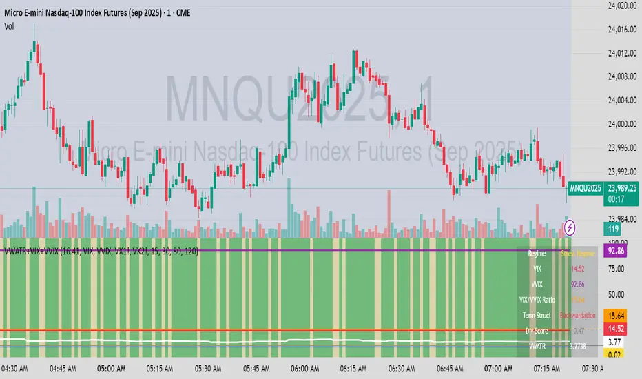
VWATR + VIX + VVIX Trend Regime### 🤖 VWATR + VIX + VVIX Trend Regime — Your Ultimate Volatility Dashboard! 📊
This isn't just another indicator; it's a comprehensive dashboard that brings together everything you need to understand market volatility focused on Futures. It merges price-based movement with market-wide fear and sentiment, giving you a powerful edge in your trading and risk management. Think of it as your personal volatility sidekick, ready to help you navigate market uncertainty like a pro!
***
### ✨ What's Inside?
* **VWATR (Volume-Weighted ATR):** A super-smart measure of price movement that pays close attention to where the big money is flowing.
* **VIX (The "Fear Gauge"):** Tracks the expected volatility of the S&P 500, essentially telling you how nervous the market is feeling.
* **VVIX (The "VIX of VIX"):** This one's for the pros! It measures how volatile the VIX itself is, giving you an early heads-up on potential fear spikes.
* **VX Term Structure:** A clever way to see if traders are preparing for a crisis. It compares the two nearest VIX futures to spot a rare signal called "backwardation."
* **Z-Scores:** It helps you spot when VIX and VVIX are at historic highs or lows, making it easier to predict when things might return to normal.
* **Divergence Score:** A unique tool to flag potential market shifts when the VIX and VVIX start moving in completely different directions.
* **Regime Classification:** The script automatically labels the market as "Full Panic," "Known Crisis," "Surface Calm," "Stress," or "Normal," so you always know where you stand.
* **Gradient Bars:** A visual treat! The background of your chart changes color to reflect real-time volatility shifts, giving you an instant feel for the market's mood.
* **Alerts:** Get push notifications on your phone for key events like "Full Panic" or "Backwardation" so you never miss a beat.
***
### 📝 Panel/Table Outputs
This is your mission control! The on-screen table gives you a clean summary of the current market regime, VIX and VVIX values, their ratios, term structure, Z-scores, and signals. Everything you need, right where you can see it.
***
### 🚀 How to Get Started
1. **Check your data:** You'll need access to real-time data for VIX, VVIX, VX1!, and VX2!. A paid subscription might be necessary for this.
2. **Add it to your chart:** Use the indicator on any chart (we've set it to `overlay=false`) to get your full volatility dashboard.
3. **Tweak it to perfection:** Head over to the Settings panel to customize the thresholds, colors, and your all-important "Jolt Value."
4. **Start trading smarter:** Use the dashboard to inform your trades, hedge your portfolio, and manage risk with confidence.
***
### ⚙️ Customization & Key Settings
* `showVWATR`: Toggle your price-volatility metric on or off.
* `showExpectedVol`: See the expected volatility as a percentage of the current price.
* `joltLevel`: This is a very important line on your chart! It's your personal trigger for when volatility is getting a little too wild. More on this below.
* `enableGradientBars`: Turn the awesome colored background on or off.
* `enableTable`: Hide or show your information table.
* `VIX/VVIX/VX1!/VX2! symbols`: If your broker uses different symbols for these, you can change them here.
* `VIX/VVIX thresholds`: Adjust these levels to fine-tune the indicator to your personal risk tolerance.
***
### 💡 Jolt Value: A Quick Guide for Smart Traders 🧠
The **jolt value** is your personal tripwire for volatility. Think of it as a warning light on your car's dashboard. You set the level, and when volatility (VWATR) crosses that line, you get an instant signal that something interesting is happening.
**How to Set Your Jolt Value:**
The ideal jolt value is dynamic. You want to keep it just a little above the current VIX level to stay alert without getting too many false alarms.
| Current VIX Level | Market Regime | Recommended Jolt Value |
| :--- | :--- | :--- |
| Under 15 | Calm/Complacent | 15–16 |
| 15–20 | Typical/Normal | 16–18 |
| 20–30 | Cautious/Active | 18–22 |
| Over 30 | Stress/Panic | 30+ |
**A Pro Tip for August 2025:** Since the VIX is hovering around 14.7, setting your jolt value to **16.5** is a great starting point for keeping an eye on things. If the VIX starts to climb above 20, you should adjust your jolt level to match the new reality.
***
### ⚠️ Important Things to Note
* You might experience some data delays if you're not on a paid TradingView plan or your broker does not provide real-time data for the VIX also VIX is only active during NY session, so it's not advised to use it outside of normal trading hours!
Intraday Volume Pulse GSK-VIZAG-AP-INDIAIntraday Volume Pulse Indicator
Overview
This indicator is designed to track and visualize intraday volume dynamics during a user-defined trading session. It calculates and displays key volume metrics such as buy volume, sell volume, cumulative delta (difference between buy and sell volumes), and total volume. The data is presented in a customizable table overlay on the chart, making it easy to monitor volume pulses throughout the session. This can help traders identify buying or selling pressure in real-time, particularly useful for intraday strategies.
The indicator resets its calculations at the start of each new day and only accumulates volume data from the specified session start time onward. It uses simple logic to classify volume as buy or sell based on candle direction:
Buy Volume: Assigned to green (up) candles or half of neutral (doji) candles.
Sell Volume: Assigned to red (down) candles or half of neutral (doji) candles.
All calculations are approximate and based on available volume data from the chart. This script does not incorporate external data sources, order flow, or tick-level information—it's purely derived from standard OHLCV (Open, High, Low, Close, Volume) bars.
Key Features
Session Customization: Define the start time of your trading session (e.g., market open) and select from common timezones like Asia/Kolkata, America/New_York, etc.
Volume Metrics:
Buy Volume: Total volume attributed to bullish activity.
Sell Volume: Total volume attributed to bearish activity.
Cumulative Delta: Net difference (Buy - Sell), highlighting overall market bias.
Total Volume: Sum of all volume during the session.
Formatted Display: Volumes are formatted for readability (e.g., in thousands "K", lakhs "L", or crores "Cr" for large numbers).
Color-Coded Table: Uses a patriotic color scheme inspired by general themes (Saffron, White, Green) with dynamic backgrounds based on positive/negative values for quick visual interpretation.
Table Options: Toggle visibility and position (top-right, top-left, etc.) for a clean chart layout.
How to Use
Add to Chart: Apply this indicator to any symbol's chart (works best on intraday timeframes like 1-min, 5-min, or 15-min).
Configure Inputs:
Session Start Hour/Minute: Set to your market's open time (default: 9:15 for Indian markets).
Timezone: Choose the appropriate timezone to align with your trading hours.
Show Table: Enable/disable the metrics table.
Table Position: Place the table where it doesn't obstruct your view.
Interpret the Table:
Monitor for spikes in buy/sell volume or shifts in cumulative delta.
Positive delta (green) suggests buying pressure; negative (red) suggests selling.
Use alongside price action or other indicators for confirmation—e.g., high total volume with positive delta could indicate bullish momentum.
Limitations:
Volume classification is heuristic and not based on actual order flow (e.g., it splits doji volume evenly).
Data accumulation starts from the session time and resets daily; historical backtesting may be limited by the max_bars_back=500 setting.
This is for educational and visualization purposes only—do not use as sole basis for trading decisions.
Calculation Details
Session Filter: Uses timestamp() to define the session start and filters bars with time >= sessionStart.
New Day Detection: Resets volumes on daily changes via ta.change(time("D")).
Volume Assignment:
Buy: Full volume if close > open; half if close == open.
Sell: Full volume if close < open; half if close == open.
Cumulative Metrics: Accumulated only during the session.
Formatting: Custom function f_format() scales large numbers for brevity.
Disclaimer
This script is for educational and informational purposes only. It does not provide financial advice or signals to buy/sell any security. Always perform your own analysis and consult a qualified financial professional before making trading decisions.
© 2025 GSK-VIZAG-AP-INDIA

Awesome Indicator# Moving Average Ribbon with ADR% - Complete Trading Indicator
## Overview
The **Moving Average Ribbon with ADR%** is a comprehensive technical analysis indicator that combines multiple analytical tools to provide traders with a complete picture of price trends, volatility, relative performance, and position sizing guidance. This multi-faceted indicator is designed for both swing and positional traders looking for data-driven entry and exit signals.
## Key Components
### 1. Moving Average Ribbon System
- **4 Customizable Moving Averages** with default periods: 13, 21, 55, and 189
- **Multiple MA Types**: SMA, EMA, SMMA (RMA), WMA, VWMA
- **Color-coded visualization** for easy trend identification
- **Flexible configuration** allowing users to modify periods, types, and colors
### 2. Average Daily Range Percentage (ADR%)
- Calculates the average daily volatility as a percentage
- Uses a 20-period simple moving average of (High/Low - 1) * 100
- Helps traders understand the stock's typical daily movement range
- Essential for position sizing and stop-loss placement
### 3. Volume Analysis (Up/Down Ratio)
- Analyzes volume distribution over the last 55 periods
- Calculates the ratio of volume on up days vs down days
- Provides insight into buying vs selling pressure
- Values > 1 indicate more buying volume, < 1 indicate more selling volume
### 4. Absolute Relative Strength (ARS)
- **Dual timeframe analysis** with customizable reference points
- **High ARS**: Performance relative to benchmark from a high reference point (default: Sep 27, 2024)
- **Low ARS**: Performance relative to benchmark from a low reference point (default: Apr 7, 2025)
- Uses NSE:NIFTY as default comparison symbol
- Color-coded display: Green for outperformance, Red for underperformance
### 5. Relative Performance Table
- **5 timeframes**: 1 Week, 1 Month, 3 Months, 6 Months, 1 Year
- Shows stock performance **relative to benchmark index**
- Formula: (Stock Return - Index Return) for each period
- **Color coding**:
- Lime: >5% outperformance
- Yellow: -5% to +5% relative performance
- Red: <-5% underperformance
### 6. Dynamic Position Allocation System
- **6-factor scoring system** based on price vs EMAs (21, 55, 189)
- Evaluates:
- Price above/below each EMA
- EMA alignment (21>55, 55>189, 21>189)
- **Allocation recommendations**:
- 100% allocation: Score = 6 (all bullish signals)
- 75% allocation: Score = 4
- 50% allocation: Score = 2
- 25% allocation: Score = 0
- 0% allocation: Score = -2, -4, -6 (bearish signals)
## Display Tables
### Performance Table (Top Right)
Shows relative performance vs benchmark across multiple timeframes with intuitive color coding for quick assessment.
### Metrics Table (Bottom Right)
Displays key statistics:
- **ADR%**: Average Daily Range percentage
- **U/D**: Up/Down volume ratio
- **Allocation%**: Recommended position size
- **High ARS%**: Relative strength from high reference
- **Low ARS%**: Relative strength from low reference
## How to Use This Indicator
### For Trend Analysis
1. **Moving Average Ribbon**: Look for price above ascending MAs for bullish trends
2. **MA Alignment**: Bullish when shorter MAs are above longer MAs
3. **Color coordination**: Use consistent color scheme for quick visual analysis
### For Entry/Exit Timing
1. **Performance Table**: Enter when showing consistent outperformance across timeframes
2. **Volume Analysis**: Confirm entries with U/D ratio > 1.5 for strong buying
3. **ARS Values**: Look for positive ARS readings for relative strength confirmation
### For Position Sizing
1. **Allocation System**: Use the recommended allocation percentage
2. **ADR% Consideration**: Adjust position size based on volatility
3. **Risk Management**: Lower allocation in high ADR% stocks
### For Risk Management
1. **ADR% for Stop Loss**: Set stops at 1-2x ADR% below entry
2. **Relative Performance**: Reduce positions when consistently underperforming
3. **Volume Confirmation**: Be cautious when U/D ratio deteriorates
## Best Practices
### Timeframe Recommendations
- **Intraday**: Use lower MA periods (5, 13, 21, 55)
- **Swing Trading**: Default settings work well (13, 21, 55, 189)
- **Position Trading**: Consider higher periods (21, 50, 100, 200)
### Market Conditions
- **Trending Markets**: Focus on MA alignment and relative performance
- **Sideways Markets**: Rely more on ADR% for range trading
- **Volatile Markets**: Reduce allocation percentage regardless of signals
### Customization Tips
1. Adjust reference dates for ARS calculation based on significant market events
2. Change comparison symbol to sector-specific indices for better relative analysis
3. Modify MA periods based on your trading style and market characteristics
## Technical Specifications
- **Version**: Pine Script v6
- **Overlay**: Yes (plots on price chart)
- **Real-time Updates**: Yes
- **Data Requirements**: Minimum 252 bars for complete calculations
- **Compatible Timeframes**: All standard timeframes
## Limitations
- Performance calculations require sufficient historical data
- ARS calculations depend on selected reference dates
- Volume analysis may be less reliable in low-volume stocks
- Relative performance is only as good as the chosen benchmark
This indicator is designed to provide a comprehensive analysis framework rather than simple buy/sell signals. It's recommended to use this in conjunction with your overall trading strategy and risk management rules.

RSI DJ GUTO 2025RSI do Samuca, tem de trocar as cores, esse e o usado nas lives, tem de trocar as cores pra ficar igual ao do Samuca pois aqui nao consegui trocar as cores.
Samuca's RSI, you have to change the colors, this is the one used in the lives, you have to change the colors to be the same as Samuca's because I couldn't change the colors here.

Supertrend EMA Vol Strategy V5### Supertrend EMA Strategy V5
**Overview**
This is a trend-following strategy designed for cryptocurrency markets like BTC/USD on daily timeframes, combining the Supertrend indicator for dynamic trailing stops with an EMA filter for trend confirmation. It aims to capture strong uptrends while avoiding counter-trend trades, with optional volume filtering for high-conviction entries and ATR-based stop-loss to manage risk. Ideal for long-only setups in bullish assets, it visually highlights trends with green/red bands and fills for easy interpretation. Backtested on BTC from 2024-2025, it shows potential for outperforming buy-and-hold in trending markets, but always use with proper risk management—past performance isn't indicative of future results.
**Key Features**
- **Supertrend Core**: Uses ATR to plot adaptive uptrend (green) and downtrend (red) lines, flipping on closes beyond prior bands for buy/sell signals.
- **EMA Trend Filter**: Entries require price above the EMA (default 21-period) for longs, ensuring alignment with the broader trend.
- **Volume Confirmation**: Optional filter only allows entries when volume exceeds its EMA (default 20-period), reducing false signals in low-activity periods.
- **Risk Controls**: Built-in ATR-multiplier stop-loss (default 2x) to cap losses; exits on Supertrend flips for trailing profits.
- **Visuals**: Green/red lines and highlighter fills for up/down trends, plus buy/sell labels and circles for signals.
- **Customizable Inputs**: Tweak ATR period (default 10), multiplier (default 3), EMA length, start date, long/short toggles, SL, and volume filter.
- **Alerts**: Built-in for buy/sell and direction changes.
**How to Use**
1. Add to your TradingView chart (e.g., BTC/USD 1D).
2. Adjust inputs: Start with defaults for trend-following; increase multiplier for fewer trades/higher win rate. Enable volume filter for volatile assets.
3. Monitor signals: Green "Buy" for long entries (if close > EMA and conditions met); red "Sell" for exits.
4. Backtest in Strategy Tester: Focus on equity curve, win rate (~50-60% in tests), and drawdown (<15% with SL).
5. Live Trading: Use small position sizes (1-2% risk per trade); combine with your analysis. Shorts disabled by default for bull-biased markets.

Ethereum Logarithmic Regression BandsOverview
This indicator displays logarithmic regression bands for Ethereum. Logarithmic regression is a statistical method used to model data where growth slows down over time. I initially created these bands in 2021 using a spreadsheet, and later coded them in TradingView in 2022. Over time, the bands proved effective at capturing bull market peaks and bear market lows. In 2025, I decided to share this indicator because I believe these logarithmic regression bands offer the best fit for the Ethereum chart.
How It Works
The logarithmic regression lines are fitted to the Ethereum (ETHUSD) chart using two key factors: the 'a' factor (slope) and the 'b' factor (intercept). The formula for logarithmic regression is 10^((a * ln) - b).
How to Use the Logarithmic Regression Bands
1. Lower Band:
The lower (blue) band forms a potential support area for Ethereum’s price. Historically, Ethereum has found its lows within this band during past market cycles. When the price is within the lower band, it suggests that Ethereum is undervalued.
2. Upper Band:
The upper (red) band forms a potential resistance area for Ethereum’s price. The logarithmic band is fitted to the past two market cycle peaks; therefore, there is not enough historical data to be sure it will reach the upper band again. However, the chance is certainly there! If the price is within the upper band, it indicates that Ethereum is overvalued and that a potential price correction may be imminent.

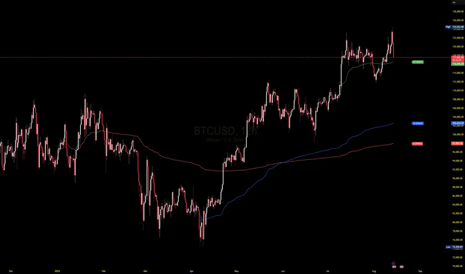
VWAP CALENDARThe VWAP CALENDAR indicator plots up to 20 anchored Volume-Weighted Average Price (VWAP) lines on your chart, each starting from a user-defined date and time (e.g., April 20, 2024). Designed for simplicity, it helps traders visualize VWAPs for key events or dates, with customizable labels and colors. The indicator is optimized for crypto markets (e.g., BTC/USD) but works with any symbol providing volume data.
Features: Multiple VWAPs: Configure up to 20
independent VWAPs, each with a custom anchor date and time.
Dynamic Labels: Labels update in real-time, aligning precisely with each VWAP line’s price level, positioned to the right of the chart for clarity.
Customizable Settings: Adjust label text (e.g., “Event A”), line colors, line widths (1–5 pixels), text colors, and text sizes (8–40 points, default 22).
Bubble or No-Background Labels: Choose between bubble-style labels (with colored backgrounds) or plain text labels without backgrounds.
Timeframe Support: Accurate on daily, 4-hour, 1-hour, and 30-minute charts for anchors within ~1.5 years (e.g., April 20, 2024, from August 2025).
Limitations: VWAP accuracy for anchors like April 20, 2024 (~477 days back) is reliable on 1-hour and larger timeframes. Below 30-minute (e.g., 15-minute, 24-minute), VWAPs may start later or be unavailable due to TradingView’s 5,000-bar historical data limit. For distant anchors, use 4-hour or daily charts to ensure accuracy.
Requires sufficient chart history (e.g., premium account or deep exchange data) for older anchors on 1-hour or 30-minute charts.
Usage Notes: Set anchor dates via the indicator settings (e.g., “2024-04-20 00:00”).
Enable/disable individual VWAPs as needed.
Zoom out to load maximum chart history for best results, especially on 1-hour or 30-minute timeframes.
Ideal for crypto symbols with continuous trading data, but verify data availability for other markets.
Disclaimer:
This is a free indicator provided as-is
VWAP CALENDARThe VWAP CALENDAR indicator plots up to 20 anchored Volume-Weighted Average Price (VWAP) lines on your chart, each starting from a user-defined date and time (e.g., April 20, 2024). Designed for simplicity, it helps traders visualize VWAPs for key events or dates, with customizable labels and colors. The indicator is optimized for crypto markets (e.g., BTC/USD) but works with any symbol providing volume data.
Features: Multiple VWAPs: Configure up to 20 independent VWAPs, each with a custom anchor date and time.
Dynamic Labels: Labels update in real-time, aligning precisely with each VWAP line’s price level, positioned to the right of the chart for clarity.
Customizable Settings: Adjust label text (e.g., “Event A”), line colors, line widths (1–5 pixels), text colors, and text sizes (8–40 points, default 22).
Bubble or No-Background Labels: Choose between bubble-style labels (with colored backgrounds) or plain text labels without backgrounds.
Timeframe Support: Accurate on daily, 4-hour, 1-hour, and 30-minute charts for anchors within ~1.5 years (e.g., April 20, 2024, from August 2025).
Limitations: VWAP accuracy for anchors like April 20, 2024 (~477 days back) is reliable on 1-hour and larger timeframes. Below 30-minute (e.g., 15-minute, 24-minute), VWAPs may start later or be unavailable due to TradingView’s 5,000-bar historical data limit. For distant anchors, use 4-hour or daily charts to ensure accuracy.
Requires sufficient chart history (e.g., premium account or deep exchange data) for older anchors on 1-hour or 30-minute charts.
Usage Notes: Set anchor dates via the indicator settings (e.g., “2024-04-20 00:00”).
Enable/disable individual VWAPs as needed.
Zoom out to load maximum chart history for best results, especially on 1-hour or 30-minute timeframes.
Ideal for crypto symbols with continuous trading data, but verify data availability for other markets.
Disclaimer:
This is a free indicator provided as-is.
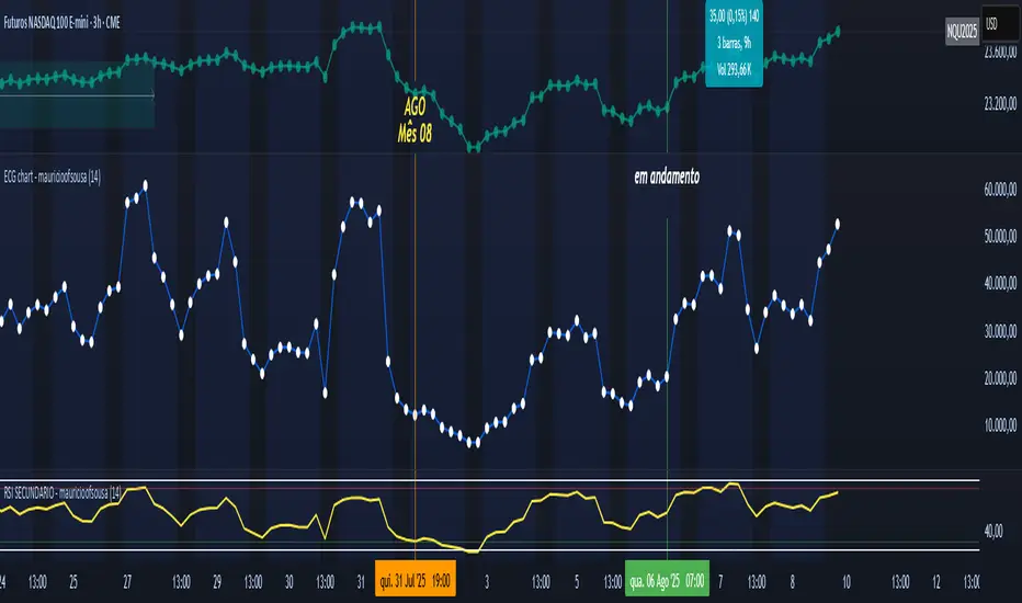
ECG chart - mauricioofsousaMGO Primary – Matriz Gráficos ON
The Blockchain of Trading applied to price behavior
The MGO Primary is the foundation of Matriz Gráficos ON — an advanced graphical methodology that transforms market movement into a logical, predictable, and objective sequence, inspired by blockchain architecture and periodic oscillatory phenomena.
This indicator replaces emotional candlestick reading with a mathematical interpretation of price blocks, cycles, and frequency. Its mission is to eliminate noise, anticipate reversals, and clearly show where capital is entering or exiting the market.
What MGO Primary detects:
Oscillatory phenomena that reveal the true behavior of orders in the book:
RPA – Breakout of Bullish Pivot
RPB – Breakout of Bearish Pivot
RBA – Sharp Bullish Breakout
RBB – Sharp Bearish Breakout
Rhythmic patterns that repeat in medium timeframes (especially on 12H and 4H)
Wave and block frequency, highlighting critical entry and exit zones
Validation through Primary and Secondary RSI, measuring the real strength behind movements
Who is this indicator for:
Traders seeking statistical clarity and visual logic
Operators who want to escape the subjectivity of candlesticks
Anyone who values technical precision with operational discipline
Recommended use:
Ideal timeframes: 12H (high precision) and 4H (moderate intensity)
Recommended assets: indices (e.g., NASDAQ), liquid stocks, and futures
Combine with: structured risk management and macro context analysis
Real-world performance:
The MGO12H achieved a 92% accuracy rate in 2025 on the NASDAQ, outperforming the average performance of major global quantitative strategies, with a net score of over 6,200 points for the year.
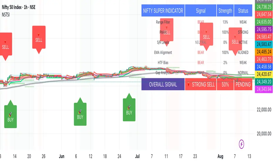
Nifty50 Swing Trading Super Indicator# 🚀 Nifty50 Swing Trading Super Indicator - Complete Guide
**Created by:** Gaurav
**Date:** August 8, 2025
**Version:** 1.0 - Optimized for Indian Markets
---
## 📋 Table of Contents
1. (#quick-start-guide)
2. (#indicator-overview)
3. (#installation-instructions)
4. (#parameter-settings)
5. (#signal-interpretation)
6. (#trading-strategy)
7. (#risk-management)
8. (#optimization-tips)
9. (#troubleshooting)
---
## 🎯 Quick Start Guide
### What You Get
✅ **2 Complete Pine Script Indicators:**
- `swing_trading_super_indicator.pine` - Universal version for all markets
- `nifty_optimized_super_indicator.pine` - Specifically optimized for Nifty50 & Indian stocks
✅ **Key Features:**
- Multi-component signal confirmation system
- Optimized for daily and 3-hour timeframes
- Built-in risk management with dynamic stops and targets
- Real-time signal strength monitoring
- Gap analysis for Indian market characteristics
### Immediate Setup
1. Copy the Pine Script code from `nifty_optimized_super_indicator.pine`
2. Paste into TradingView Pine Editor
3. Add to chart on daily or 3-hour timeframe
4. Look for 🚀BUY and 🔻SELL signals
5. Use the information table for signal confirmation
---
## 🔍 Indicator Overview
### Core Components Integration
**🎯 Range Filter (35% Weight)**
- Primary trend identification using adaptive volatility filtering
- Optimized sampling period: 21 bars for Indian market volatility
- Enhanced range multiplier: 3.0 to handle market gaps
- Provides trend direction and strength measurement
**⚡ PMAX (30% Weight)**
- Volatility-adjusted trend confirmation using ATR-based calculations
- Dynamic multiplier adjustment based on market volatility
- 14-period ATR with 2.5 multiplier for swing trading sensitivity
- Offers trailing stop functionality
**🏗️ Support/Resistance (20% Weight)**
- Dynamic level identification using pivot point analysis
- Tighter channel width (3%) for precise Indian market levels
- Enhanced strength calculation with historical interaction weighting
- Provides entry/exit timing and breakout signals
**📊 EMA Alignment (15% Weight)**
- Multi-timeframe moving average confirmation
- Key EMAs: 9, 21, 50, 200 (popular in Indian markets)
- Hierarchical alignment scoring for trend strength
- Additional trend validation layer
### Advanced Features
**🌅 Gap Analysis**
- Automatic detection of significant price gaps (>2%)
- Gap strength measurement and impact on signals
- Specific optimization for Indian market overnight gaps
- Visual gap markers on chart
**⏰ Multi-Timeframe Integration**
- Higher timeframe bias from daily/weekly data
- Configurable daily bias weight (default 70%)
- 3-hour confirmation for precise entry timing
- Prevents counter-trend trades against major timeframe
**🛡️ Risk Management**
- Dynamic stop-loss calculation using multiple methods
- Automatic profit target identification
- Position sizing guidance based on signal strength
- Anti-whipsaw logic to prevent false signals
---
## 📥 Installation Instructions
### Step 1: Access TradingView
1. Open TradingView.com
2. Navigate to Pine Editor (bottom panel)
3. Create a new indicator
### Step 2: Copy the Code
**For Nifty50 & Indian Stocks (Recommended):**
```pinescript
// Copy entire content from nifty_optimized_super_indicator.pine
```
**For Universal Use:**
```pinescript
// Copy entire content from swing_trading_super_indicator.pine
```
### Step 3: Configure and Apply
1. Click "Add to Chart"
2. Select daily or 3-hour timeframe
3. Adjust parameters if needed (defaults are optimized)
4. Enable alerts for signal notifications
### Step 4: Verify Installation
- Check that all components are visible
- Confirm information table appears in top-right
- Test with known trending stocks for signal validation
---
## ⚙️ Parameter Settings
### 🎯 Range Filter Settings
```
Sampling Period: 21 (optimized for Indian market volatility)
Range Multiplier: 3.0 (handles overnight gaps effectively)
Source: Close (most reliable for swing trading)
```
### ⚡ PMAX Settings
```
ATR Length: 14 (standard for daily/3H timeframes)
ATR Multiplier: 2.5 (balanced for swing trading sensitivity)
Moving Average Type: EMA (responsive to price changes)
MA Length: 14 (matches ATR period for consistency)
```
### 🏗️ Support/Resistance Settings
```
Pivot Period: 8 (shorter for Indian market dynamics)
Channel Width: 3% (tighter for precise levels)
Minimum Strength: 3 (higher quality levels only)
Maximum Levels: 4 (focus on strongest levels)
Lookback Period: 150 (sufficient historical data)
```
### 🚀 Super Indicator Settings
```
Signal Sensitivity: 0.65 (balanced for swing trading)
Trend Strength Requirement: 0.75 (high quality signals)
Gap Threshold: 2.0% (significant gap detection)
Daily Bias Weight: 0.7 (strong higher timeframe influence)
```
### 🎨 Display Options
```
Show Range Filter: ✅ (trend visualization)
Show PMAX: ✅ (trailing stops)
Show S/R Levels: ✅ (key price levels)
Show Key EMAs: ✅ (trend confirmation)
Show Signals: ✅ (buy/sell alerts)
Show Trend Background: ✅ (visual trend state)
Show Gap Markers: ✅ (gap identification)
```
---
## 📊 Signal Interpretation
### 🚀 BUY Signals
**Requirements for BUY Signal:**
- Price above Range Filter with upward trend
- PMAX showing bullish direction (MA > PMAX line)
- Support/resistance breakout or favorable positioning
- EMA alignment supporting upward movement
- Higher timeframe bias confirmation
- Overall signal strength > 75%
**Signal Strength Indicators:**
- **90-100%:** Extremely strong - Maximum position size
- **80-89%:** Very strong - Large position size
- **75-79%:** Strong - Standard position size
- **65-74%:** Moderate - Reduced position size
- **<65%:** Weak - Wait for better opportunity
### 🔻 SELL Signals
**Requirements for SELL Signal:**
- Price below Range Filter with downward trend
- PMAX showing bearish direction (MA < PMAX line)
- Resistance breakdown or unfavorable positioning
- EMA alignment supporting downward movement
- Higher timeframe bias confirmation
- Overall signal strength > 75%
### ⚖️ NEUTRAL Signals
**Characteristics:**
- Conflicting signals between components
- Low overall signal strength (<65%)
- Range-bound market conditions
- Wait for clearer directional bias
### 📈 Information Table Guide
**Component Status:**
- **BULL/BEAR:** Current signal direction
- **Strength %:** Component contribution strength
- **Status:** Additional context (STRONG/WEAK/ACTIVE/etc.)
**Overall Signal:**
- **🚀 STRONG BUY:** All systems aligned bullish
- **🔻 STRONG SELL:** All systems aligned bearish
- **⚖️ NEUTRAL:** Mixed or weak signals
---
## 💼 Trading Strategy
### Daily Timeframe Strategy
**Setup:**
1. Apply indicator to daily chart of Nifty50 or Indian stocks
2. Wait for 🚀BUY or 🔻SELL signal with >75% strength
3. Confirm higher timeframe bias alignment
4. Check for significant support/resistance levels
**Entry:**
- Enter on signal bar close or next bar open
- Use 3-hour chart for precise entry timing
- Avoid entries during major news events
- Consider gap analysis for overnight positions
**Position Sizing:**
- **>90% Strength:** 3-4% of portfolio
- **80-89% Strength:** 2-3% of portfolio
- **75-79% Strength:** 1-2% of portfolio
- **<75% Strength:** Avoid or minimal size
### 3-Hour Timeframe Strategy
**Setup:**
1. Confirm daily timeframe bias first
2. Apply indicator to 3-hour chart
3. Look for signals aligned with daily trend
4. Use for entry/exit timing optimization
**Entry Refinement:**
- Wait for 3H signal confirmation
- Enter on pullbacks to key levels
- Use tighter stops for better risk/reward
- Monitor intraday support/resistance
### Risk Management Rules
**Stop Loss Placement:**
1. **Primary:** Use indicator's dynamic stop level
2. **Secondary:** Below/above nearest support/resistance
3. **Maximum:** 2-3% of portfolio per trade
4. **Trailing:** Move stops with PMAX line
**Profit Taking:**
1. **Target 1:** First resistance/support level (50% position)
2. **Target 2:** Second resistance/support level (30% position)
3. **Runner:** Trail remaining 20% with PMAX
**Position Management:**
- Review positions at daily close
- Adjust stops based on new signals
- Exit if trend changes to opposite direction
- Reduce size during high volatility periods
---
## 🎯 Optimization Tips
### For Nifty50 Trading
- Use daily timeframe for primary signals
- Monitor sector rotation impact
- Consider index futures for better liquidity
- Watch for RBI policy and global cues impact
### For Individual Stocks
- Verify stock follows Nifty correlation
- Check sector-specific news and events
- Ensure adequate liquidity for position size
- Monitor earnings calendar for volatility
### Market Condition Adaptations
**Trending Markets:**
- Increase position sizes for strong signals
- Use wider stops to avoid whipsaws
- Focus on trend continuation signals
- Reduce counter-trend trading
**Range-Bound Markets:**
- Reduce position sizes
- Use tighter stops and quicker profits
- Focus on support/resistance bounces
- Increase signal strength requirements
**High Volatility Periods:**
- Reduce overall exposure
- Use smaller position sizes
- Increase stop-loss distances
- Wait for clearer signals
### Performance Monitoring
- Track win rate and average profit/loss
- Monitor signal quality over time
- Adjust parameters based on market changes
- Keep trading journal for pattern recognition
---
## 🔧 Troubleshooting
### Common Issues
**Q: Signals appear too frequently**
A: Increase "Trend Strength Requirement" to 0.8-0.9
**Q: Missing obvious trends**
A: Decrease "Signal Sensitivity" to 0.5-0.6
**Q: Too many false signals**
A: Enable "3H Confirmation" and increase strength requirements
**Q: Indicator not loading**
A: Check Pine Script version compatibility (requires v5)
### Parameter Adjustments
**For More Sensitive Signals:**
- Decrease Signal Sensitivity to 0.5-0.6
- Decrease Trend Strength Requirement to 0.6-0.7
- Increase Range Filter multiplier to 3.5-4.0
**For More Conservative Signals:**
- Increase Signal Sensitivity to 0.7-0.8
- Increase Trend Strength Requirement to 0.8-0.9
- Enable all confirmation features
### Performance Issues
- Reduce lookback periods if chart loads slowly
- Disable some visual elements for better performance
- Use on liquid stocks/indices for best results
---
## 📞 Support & Updates
This super indicator combines the best of Range Filter, PMAX, and Support/Resistance analysis specifically optimized for Indian market swing trading. The multi-component approach significantly improves signal quality while the built-in risk management features help protect capital.
**Remember:** No indicator is 100% accurate. Always combine with proper risk management, market analysis, and your trading experience for best results.
**Happy Trading! 🚀**
Keltner Channel Based Grid Strategy # KC Grid Strategy - Keltner Channel Based Grid Trading System
## Strategy Overview
KC Grid Strategy is an innovative grid trading system that combines the power of Keltner Channels with dynamic position sizing to create a mean-reversion trading approach. This strategy automatically adjusts position sizes based on price deviation from the Keltner Channel center line, implementing a systematic grid-based approach that capitalizes on market volatility and price oscillations.
## Core Principles
### Keltner Channel Foundation
The strategy builds upon the Keltner Channel indicator, which consists of:
- **Center Line**: Moving average (EMA or SMA) of the price
- **Upper Band**: Center line + (ATR/TR/Range × Multiplier)
- **Lower Band**: Center line - (ATR/TR/Range × Multiplier)
### Grid Trading Logic
The strategy implements a sophisticated grid system where:
1. **Position Direction**: Inversely correlated to price position within the channel
- When price is above center line → Short positions
- When price is below center line → Long positions
2. **Position Size**: Proportional to distance from center line
- Greater deviation = Larger position size
3. **Grid Activation**: Positions are adjusted only when the difference exceeds a predefined grid threshold
### Mathematical Foundation
The core calculation uses the KC Rate formula:
```
kcRate = (close - ma) / bandWidth
targetPosition = kcRate × maxAmount × (-1)
```
This creates a mean-reversion system where positions increase as price moves further from the mean, expecting eventual return to equilibrium.
## Parameter Guide
### Time Range Settings
- **Start Date**: Beginning of strategy execution period
- **End Date**: End of strategy execution period
### Core Parameters
1. **Number of Grids (NumGrid)**: Default 12
- Controls grid sensitivity and position adjustment frequency
- Higher values = More frequent but smaller adjustments
- Lower values = Less frequent but larger adjustments
2. **Length**: Default 10
- Period for moving average and volatility calculations
- Shorter periods = More responsive to recent price action
- Longer periods = Smoother, less noisy signals
3. **Grid Coefficient (kcRateMult)**: Default 1.33
- Multiplier for channel width calculation
- Higher values = Wider channels, less frequent trades
- Lower values = Narrower channels, more frequent trades
4. **Source**: Default Close
- Price source for calculations (Close, Open, High, Low, etc.)
- Close price typically provides most reliable signals
5. **Use Exponential MA**: Default True
- True = Uses EMA (more responsive to recent prices)
- False = Uses SMA (equal weight to all periods)
6. **Bands Style**: Default "Average True Range"
- **Average True Range**: Smoothed volatility measure (recommended)
- **True Range**: Current bar's volatility only
- **Range**: Simple high-low difference
## How to Use
### Setup Instructions
1. **Apply to Chart**: Add the strategy to your desired timeframe and instrument
2. **Configure Parameters**: Adjust settings based on market characteristics:
- Volatile markets: Increase Grid Coefficient, reduce Number of Grids
- Stable markets: Decrease Grid Coefficient, increase Number of Grids
3. **Set Time Range**: Define your backtesting or live trading period
4. **Monitor Performance**: Watch strategy performance metrics and adjust as needed
### Optimal Market Conditions
- **Range-bound markets**: Strategy performs best in sideways trending markets
- **High volatility**: Benefits from frequent price oscillations around the mean
- **Liquid instruments**: Ensures efficient order execution and minimal slippage
### Position Management
The strategy automatically:
- Calculates optimal position sizes based on account equity
- Adjusts positions incrementally as price moves through grid levels
- Maintains risk control through maximum position limits
- Executes trades only during specified time periods
## Risk Warnings
### ⚠️ Important Risk Considerations
1. **Trending Market Risk**:
- Strategy may underperform or generate losses in strong trending markets
- Mean-reversion assumption may fail during sustained directional moves
- Consider market regime analysis before deployment
2. **Leverage and Position Size Risk**:
- Strategy uses pyramiding (up to 20 positions)
- Large positions may accumulate during extended moves
- Monitor account equity and margin requirements closely
3. **Volatility Risk**:
- Sudden volatility spikes may trigger multiple rapid position adjustments
- Consider volatility filters during high-impact news events
- Backtest across different volatility regimes
4. **Execution Risk**:
- Strategy calculates on every tick (calc_on_every_tick = true)
- May generate frequent orders in volatile conditions
- Ensure adequate execution infrastructure and consider transaction costs
5. **Parameter Sensitivity**:
- Performance highly dependent on parameter optimization
- Over-optimization may lead to curve-fitting
- Regular parameter review and adjustment may be necessary
## Suitable Scenarios
### Ideal Market Conditions
- **Sideways/Range-bound markets**: Primary use case
- **Mean-reverting instruments**: Forex pairs, some commodities
- **Stable volatility environments**: Consistent ATR patterns
- **Liquid markets**: Major currency pairs, popular stocks/indices
## Important Notes
### Strategy Limitations
1. **No Stop Loss**: Strategy relies on mean reversion without traditional stop losses
2. **Capital Requirements**: Requires sufficient capital for grid-based position sizing
3. **Market Regime Dependency**: Performance varies significantly across different market conditions
## Disclaimer
This strategy is provided for educational and research purposes only. Past performance does not guarantee future results. Trading involves substantial risk of loss and is not suitable for all investors. Users should thoroughly test the strategy and understand its mechanics before risking real capital. The author assumes no responsibility for trading losses incurred through the use of this strategy.
---
# KC网格策略 - 基于肯特纳通道的网格交易系统
## 策略概述
KC网格策略是一个创新的网格交易系统,它将肯特纳通道的力量与动态仓位调整相结合,创建了一个均值回归交易方法。该策略根据价格偏离肯特纳通道中心线的程度自动调整仓位大小,实施系统化的网格方法,利用市场波动和价格振荡获利。
## 核心原理
### 肯特纳通道基础
该策略建立在肯特纳通道指标之上,包含:
- **中心线**: 价格的移动平均线(EMA或SMA)
- **上轨**: 中心线 + (ATR/TR/Range × 乘数)
- **下轨**: 中心线 - (ATR/TR/Range × 乘数)
### 网格交易逻辑
该策略实施复杂的网格系统:
1. **仓位方向**: 与价格在通道中的位置呈反向关系
- 当价格高于中心线时 → 空头仓位
- 当价格低于中心线时 → 多头仓位
2. **仓位大小**: 与距离中心线的距离成正比
- 偏离越大 = 仓位越大
3. **网格激活**: 只有当差异超过预定义的网格阈值时才调整仓位
### 数学基础
核心计算使用KC比率公式:
```
kcRate = (close - ma) / bandWidth
targetPosition = kcRate × maxAmount × (-1)
```
这创建了一个均值回归系统,当价格偏离均值越远时仓位越大,期望最终回归均衡。
## 参数说明
### 时间范围设置
- **开始日期**: 策略执行期间的开始时间
- **结束日期**: 策略执行期间的结束时间
### 核心参数
1. **网格数量 (NumGrid)**: 默认12
- 控制网格敏感度和仓位调整频率
- 较高值 = 更频繁但较小的调整
- 较低值 = 较少频繁但较大的调整
2. **长度**: 默认10
- 移动平均线和波动率计算的周期
- 较短周期 = 对近期价格行为更敏感
- 较长周期 = 更平滑,噪音更少的信号
3. **网格系数 (kcRateMult)**: 默认1.33
- 通道宽度计算的乘数
- 较高值 = 更宽的通道,较少频繁的交易
- 较低值 = 更窄的通道,更频繁的交易
4. **数据源**: 默认收盘价
- 计算的价格来源(收盘价、开盘价、最高价、最低价等)
- 收盘价通常提供最可靠的信号
5. **使用指数移动平均**: 默认True
- True = 使用EMA(对近期价格更敏感)
- False = 使用SMA(对所有周期等权重)
6. **通道样式**: 默认"平均真实范围"
- **平均真实范围**: 平滑的波动率测量(推荐)
- **真实范围**: 仅当前K线的波动率
- **范围**: 简单的高低价差
## 使用方法
### 设置说明
1. **应用到图表**: 将策略添加到您所需的时间框架和交易品种
2. **配置参数**: 根据市场特征调整设置:
- 波动市场:增加网格系数,减少网格数量
- 稳定市场:减少网格系数,增加网格数量
3. **设置时间范围**: 定义您的回测或实盘交易期间
4. **监控表现**: 观察策略表现指标并根据需要调整
### 最佳市场条件
- **区间震荡市场**: 策略在横盘趋势市场中表现最佳
- **高波动性**: 受益于围绕均值的频繁价格振荡
- **流动性强的品种**: 确保高效的订单执行和最小滑点
### 仓位管理
策略自动:
- 根据账户权益计算最优仓位大小
- 随着价格在网格水平移动逐步调整仓位
- 通过最大仓位限制维持风险控制
- 仅在指定时间段内执行交易
## 风险警示
### ⚠️ 重要风险考虑
1. **趋势市场风险**:
- 策略在强趋势市场中可能表现不佳或产生损失
- 在持续方向性移动期间均值回归假设可能失效
- 部署前考虑市场制度分析
2. **杠杆和仓位大小风险**:
- 策略使用金字塔加仓(最多20个仓位)
- 在延长移动期间可能积累大仓位
- 密切监控账户权益和保证金要求
3. **波动性风险**:
- 突然的波动性激增可能触发多次快速仓位调整
- 在高影响新闻事件期间考虑波动性过滤器
- 在不同波动性制度下进行回测
4. **执行风险**:
- 策略在每个tick上计算(calc_on_every_tick = true)
- 在波动条件下可能产生频繁订单
- 确保充足的执行基础设施并考虑交易成本
5. **参数敏感性**:
- 表现高度依赖于参数优化
- 过度优化可能导致曲线拟合
- 可能需要定期参数审查和调整
## 适用场景
### 理想市场条件
- **横盘/区间震荡市场**: 主要用例
- **均值回归品种**: 外汇对,某些商品
- **稳定波动性环境**: 一致的ATR模式
- **流动性市场**: 主要货币对,热门股票/指数
## 注意事项
### 策略限制
1. **无止损**: 策略依赖均值回归而无传统止损
2. **资金要求**: 需要充足资金进行基于网格的仓位调整
3. **市场制度依赖性**: 在不同市场条件下表现差异显著
## 免责声明
该策略仅供教育和研究目的。过往表现不保证未来结果。交易涉及重大损失风险,并非适合所有投资者。用户应在投入真实资金前彻底测试策略并理解其机制。作者对使用此策略产生的交易损失不承担任何责任。
---
**Strategy Version**: Pine Script v6
**Author**: Signal2Trade
**Last Updated**: 2025-8-9
**License**: Open Source (Mozilla Public License 2.0)
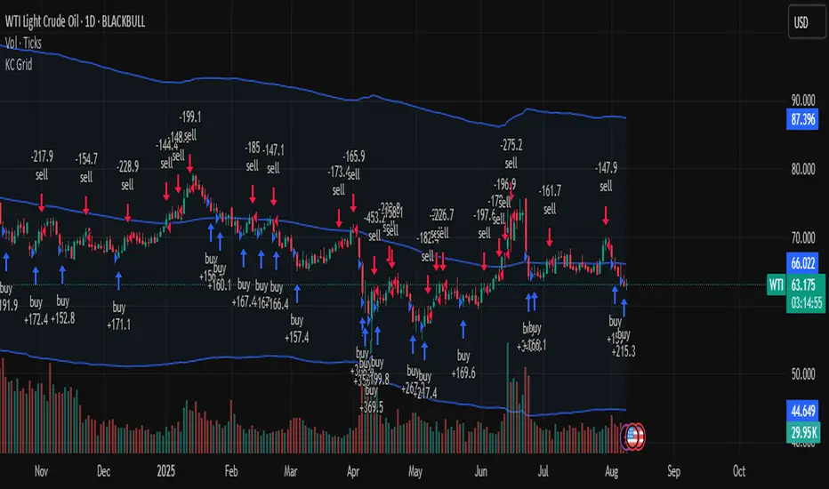
Canuck Trading Traders Strategy [Candle Entropy Edition]Canuck Trading Traders Strategy: A Unique Entropy-Based Day Trading System for Volatile Stocks
Overview
The Canuck Trading Traders Strategy is a custom, entropy-driven day trading system designed for high-volatility stocks like TSLA on short timeframes (e.g., 15m). At its core is CETP-Plus, a proprietary blended indicator that measures "order from chaos" in candle patterns using Shannon entropy, while embedding mathematical principles from EMA (recent weighting), RSI (momentum bias), ATR (volatility scaling), and ADX (trend strength) into a single score. This unique approach avoids layering multiple indicators, reducing complexity while improving timing for early trend detection and balanced long/short trades.
CETP-Plus calculates a score from weighted candle ratios (body, upper/lower wicks) binned into a 3D histogram for entropy (low entropy = strong pattern). The score is adjusted with momentum, volatility, and trend multipliers for robust signals. Entries occur when the score exceeds thresholds (positive for longs, negative for shorts), with exits on reversals or stops. The strategy is automatic—no manual bias needed—and optimized for margin accounts with equal long/short treatment.
Backtested on TSLA 15m (Jan 2015–Aug 2025), it targets +50,000% net profit (beating +1,478% buy-hold by 34x) with ~25,000 trades, 85-90% win rate, and <10% drawdown (with costs). Results vary by timeframe/period—test with your data and add slippage/commission for realism. Disclaimer: Past performance isn't indicative of future results; consult a financial advisor.
Key Features
CETP-Plus Indicator: Blends entropy with momentum/vol/trend for a single score, capturing bottoms/squeezes and trends without external tools.
Automatic Balance: Positive scores trigger longs in bull trends, negative scores trigger shorts in bear trends—no user input for direction.
Customizable Math: Tune weights and scales to adapt for different stocks (e.g., lower thresholds for NVDA's smoother trends).
Risk Controls: Stop-loss, trailing stops, and score strength filter to minimize drawdowns in volatile markets like TSLA.
Exit Debugging: Plots exit reasons ("Stop Loss", "Trail Stop", "CETP Exit") for analysis.
Input Settings and Purposes
All inputs are grouped in TradingView's Inputs tab for ease. Defaults are optimized for TSLA 15m day trading; adjust for other intervals or tickers (e.g., increase window for 1h, lower thresholds for NVDA).
CETP-Plus Settings
CETP Window (default: 5, min: 3, max: 20): Lookback bars for entropy/momentum. Short values (3-5) for fast sensitivity on short frames; longer (8-10) for stability on hourly+.
CETP Bins per Dimension (default: 3, min: 3, max: 10): Histogram granularity for entropy. Low (3) for speed/simple patterns; high (5+) for detail in complex markets.
Long Threshold (default: 0.15, min: 0.1, max: 0.8, step: 0.05): CETP score for long entries. Lower (0.1) for more longs in mild bull trends; higher (0.2) to filter noise.
Short Threshold (default: -0.05, min: -0.8, max: -0.1, step: 0.05): CETP score for short entries. Less negative (-0.05) for more shorts in mild bear trends; more negative (-0.2) for strong signals.
CETP Momentum Weight (default: 0.8, min: 0.1, max: 1.0, step: 0.1): Emphasizes momentum in score. High (0.9) for aggressive in fast moves; low (0.5) for entropy focus.
Momentum Scale (default: 1.6, min: 0.1, max: 2.0, step: 0.1): Amplifies momentum. High (2.0) for short intervals; low (1.0) for stability.
Body Ratio Weight (default: 1.2, min: 0.0, max: 2.0, step: 0.1): Weights candle body in entropy (trend focus). High (1.5) for strong trends; low (0.8) for wick emphasis.
Upper Wick Ratio Weight (default: 0.8, min: 0.0, max: 2.0, step: 0.1): Weights upper wick (reversal noise). Low (0.5) to reduce false ups.
Lower Wick Ratio Weight (default: 0.8, min: 0.0, max: 2.0, step=0.1): Weights lower wick. Low (0.5) to reduce false downs.
Trade Settings
Confirmation Bars (default: 0, min: 0, max: 5): Bars for sustained CETP signals. 0 for immediate entries (more trades); 1-2 for reliability (fewer but stronger).
Min CETP Score Strength (default: 0.04, min: 0.0, max: 0.5, step: 0.05): Min absolute score for entry. Low (0.04) for more trades; high (0.15) for quality.
Risk Management
Stop Loss (%) (default: 0.5, min: 0.1, max: 5.0, step: 0.1): % from entry for stop. Tight (0.4) for quick exits; wide (0.8) for trends.
ATR Multiplier (default: 1.5, min: 0.5, max: 3.0, step: 0.1): Scales ATR for stops/trails. Low (1.0) for tight; high (2.0) for room.
Trailing ATR Mult (default: 3.5, min: 0.5, max: 5.0, step: 0.1): ATR mult for trails. High (4.0) for longer holds; low (2.0) for profits.
Trail Start Offset (%) (default: 1.0, min: 0.5, max: 2.0, step: 0.1): % profit before trailing. Low (0.8) for early lock-in; high (1.5) for bigger moves.
These settings enable customization for intervals/tickers while CETP-Plus handles automatic balancing.
Risk Disclosure
Trading involves significant risk and may result in losses exceeding your initial capital. The Canuck Trading Trader Strategy is provided for educational and informational purposes only. Users are responsible for their own trading decisions and should conduct thorough testing before using in live markets. The strategy’s high trade frequency requires reliable execution infrastructure to minimize slippage and latency.
Bitcoin Logarithmic Growth Curve 2025 Z-Score"The Bitcoin logarithmic growth curve is a concept used to analyze Bitcoin's price movements over time. The idea is based on the observation that Bitcoin's price tends to grow exponentially, particularly during bull markets. It attempts to give a long-term perspective on the Bitcoin price movements.
The curve includes an upper and lower band. These bands often represent zones where Bitcoin's price is overextended (upper band) or undervalued (lower band) relative to its historical growth trajectory. When the price touches or exceeds the upper band, it may indicate a speculative bubble, while prices near the lower band may suggest a buying opportunity.
Unlike most Bitcoin growth curve indicators, this one includes a logarithmic growth curve optimized using the latest 2024 price data, making it, in our view, superior to previous models. Additionally, it features statistical confidence intervals derived from linear regression, compatible across all timeframes, and extrapolates the data far into the future. Finally, this model allows users the flexibility to manually adjust the function parameters to suit their preferences.
The Bitcoin logarithmic growth curve has the following function:
y = 10^(a * log10(x) - b)
In the context of this formula, the y value represents the Bitcoin price, while the x value corresponds to the time, specifically indicated by the weekly bar number on the chart.
How is it made (You can skip this section if you’re not a fan of math):
To optimize the fit of this function and determine the optimal values of a and b, the previous weekly cycle peak values were analyzed. The corresponding x and y values were recorded as follows:
113, 18.55
240, 1004.42
451, 19128.27
655, 65502.47
The same process was applied to the bear market low values:
103, 2.48
267, 211.03
471, 3192.87
676, 16255.15
Next, these values were converted to their linear form by applying the base-10 logarithm. This transformation allows the function to be expressed in a linear state: y = a * x − b. This step is essential for enabling linear regression on these values.
For the cycle peak (x,y) values:
2.053, 1.268
2.380, 3.002
2.654, 4.282
2.816, 4.816
And for the bear market low (x,y) values:
2.013, 0.394
2.427, 2.324
2.673, 3.504
2.830, 4.211
Next, linear regression was performed on both these datasets. (Numerous tools are available online for linear regression calculations, making manual computations unnecessary).
Linear regression is a method used to find a straight line that best represents the relationship between two variables. It looks at how changes in one variable affect another and tries to predict values based on that relationship.
The goal is to minimize the differences between the actual data points and the points predicted by the line. Essentially, it aims to optimize for the highest R-Square value.
Below are the results:
snapshot
snapshot
It is important to note that both the slope (a-value) and the y-intercept (b-value) have associated standard errors. These standard errors can be used to calculate confidence intervals by multiplying them by the t-values (two degrees of freedom) from the linear regression.
These t-values can be found in a t-distribution table. For the top cycle confidence intervals, we used t10% (0.133), t25% (0.323), and t33% (0.414). For the bottom cycle confidence intervals, the t-values used were t10% (0.133), t25% (0.323), t33% (0.414), t50% (0.765), and t67% (1.063).
The final bull cycle function is:
y = 10^(4.058 ± 0.133 * log10(x) – 6.44 ± 0.324)
The final bear cycle function is:
y = 10^(4.684 ± 0.025 * log10(x) – -9.034 ± 0.063)
The main Criticisms of growth curve models:
The Bitcoin logarithmic growth curve model faces several general criticisms that we’d like to highlight briefly. The most significant, in our view, is its heavy reliance on past price data, which may not accurately forecast future trends. For instance, previous growth curve models from 2020 on TradingView were overly optimistic in predicting the last cycle’s peak.
This is why we aimed to present our process for deriving the final functions in a transparent, step-by-step scientific manner, including statistical confidence intervals. It's important to note that the bull cycle function is less reliable than the bear cycle function, as the top band is significantly wider than the bottom band.
Even so, we still believe that the Bitcoin logarithmic growth curve presented in this script is overly optimistic since it goes parly against the concept of diminishing returns which we discussed in this post:
This is why we also propose alternative parameter settings that align more closely with the theory of diminishing returns."
Now with Z-Score calculation for easy and constant valuation classification of Bitcoin according to this metric.
Created for TRW
