Opening Range Breakout with Multi-Timeframe Liquidity]═══════════════════════════════════════
OPENING RANGE BREAKOUT WITH MULTI-TIMEFRAME LIQUIDITY
═══════════════════════════════════════
A professional Opening Range Breakout (ORB) indicator enhanced with multi-timeframe liquidity detection, trading session visualization, volume analysis, and trend confirmation tools. Designed for intraday trading with comprehensive alert system.
───────────────────────────────────────
WHAT THIS INDICATOR DOES
───────────────────────────────────────
This indicator combines multiple trading concepts:
- Opening Range Breakout (ORB) - Customizable time period detection with automatic high/low identification
- Multi-Timeframe Liquidity - HTF (Higher Timeframe) and LTF (Lower Timeframe) key level detection
- Trading Sessions - Tokyo, London, New York, and Sydney session visualization
- Volume Analysis - Volume spike detection and strength measurement
- Multi-Timeframe Confirmation - Trend bias from higher timeframes
- EMA Integration - Trend filter and dynamic support/resistance
- Smart Alerts - Quality-filtered breakout notifications
───────────────────────────────────────
HOW IT WORKS
───────────────────────────────────────
OPENING RANGE BREAKOUT (ORB):
Concept:
The Opening Range is a period at the start of a trading session where price establishes an initial high and low. Breakouts beyond this range often indicate the direction of the day's trend.
Detection Method:
- Default: 15-minute opening range (configurable)
- Custom Range: Set specific session times with timezone support
- Automatically identifies ORH (Opening Range High) and ORL (Opening Range Low)
- Tracks ORB mid-point for reference
Range Establishment:
1. Session starts (or custom time begins)
2. Tracks highest high and lowest low during the period
3. Range confirmed at end of opening period
4. Levels extend throughout the session
Breakout Detection:
- Bullish Breakout: Close above ORH
- Bearish Breakout: Close below ORL
- Mid-point acts as bias indicator
Visual Display:
- Shaded box during range formation
- Horizontal lines for ORH, ORL, and mid-point
- Labels showing level values
- Color-coded fills based on selected method
Fill Color Methods:
1. Session Comparison:
- Green: Current OR mid > Previous OR mid
- Red: Current OR mid < Previous OR mid
- Gray: Equal or first session
- Shows day-over-day momentum
2. Breakout Direction (Recommended):
- Green: Price currently above ORH (bullish breakout)
- Red: Price currently below ORL (bearish breakout)
- Gray: Price inside range (no breakout)
- Real-time breakout status
MULTI-TIMEFRAME LIQUIDITY:
Two-Tier System for comprehensive level identification:
HTF (Higher Timeframe) Key Liquidity:
- Default: 4H timeframe (configurable to Daily, Weekly)
- Identifies major institutional levels
- Uses pivot detection with adjustable parameters
- Suitable for swing highs/lows where large orders rest
LTF (Lower Timeframe) Key Liquidity:
- Default: 1H timeframe (configurable)
- Provides precision entry/exit levels
- Finer granularity for intraday trading
- Captures minor swing points
Calculation Method:
- Pivot high/low detection algorithm
- Configurable left bars (lookback) and right bars (confirmation)
- Timeframe multiplier for accurate multi-timeframe detection
- Automatic level extension
Mitigation System:
- Tracks when levels are swept (broken)
- Configurable mitigation type: Wick or Close-based
- Option to remove or show mitigated levels
- Display limit prevents chart clutter
Asset-Specific Optimization:
The indicator includes quick reference settings for different assets:
- Major Forex (EUR/USD, GBP/USD): Default settings optimal
- Crypto (BTC/ETH): Left=12, Right=4, Display=7
- Gold: HTF=1D, Left=20
TRADING SESSIONS:
Four Major Sessions with Full Customization:
Tokyo Session:
- Default: 04:00-13:00 UTC+4
- Asian trading hours
- Often sets daily range
London Session:
- Default: 11:00-20:00 UTC+4
- Highest liquidity period
- Major institutional activity
New York Session:
- Default: 16:00-01:00 UTC+4
- US market hours
- High-impact news events
Sydney Session:
- Default: 01:00-10:00 UTC+4
- Earliest Asian activity
- Lower volatility
Session Features:
- Shaded background boxes
- Session name labels
- Optional open/close lines
- Session high/low tracking with colored lines
- Each session has independent color settings
- Fully customizable times and timezones
VOLUME ANALYSIS:
Volume-Based Trade Confirmation:
Volume MA:
- Configurable period (default: 20)
- Establishes average volume baseline
- Used for spike detection
Volume Spike Detection:
- Identifies when volume exceeds MA * multiplier
- Default: 1.5x average volume
- Confirms breakout strength
Volume Strength Measurement:
- Calculates current volume as percentage of average
- Shows relative volume intensity
- Used in alert quality filtering
High Volume Bars:
- Identifies bars above 50th percentile
- Additional confirmation layer
- Indicates institutional participation
MULTI-TIMEFRAME CONFIRMATION:
Trend Bias from Higher Timeframes:
HTF 1 (Trend):
- Default: 1H timeframe
- Uses EMA to determine intermediate trend
- Compares current timeframe EMA to HTF EMA
HTF 2 (Bias):
- Default: 4H timeframe
- Uses 50 EMA for longer-term bias
- Confirms overall market direction
Bias Classifications:
- Bullish Bias: HTF close > HTF 50 EMA AND Current EMA > HTF1 EMA
- Bearish Bias: HTF close < HTF 50 EMA AND Current EMA < HTF1 EMA
- Neutral Bias: Mixed signals between timeframes
EMA Stack Analysis:
- Compares EMA alignment across timeframes
- +1: Bullish stack (lower TF EMA > higher TF EMA)
- -1: Bearish stack (lower TF EMA < higher TF EMA)
- 0: Neutral/crossed
Usage:
- Filters false breakouts
- Confirms trend direction
- Improves trade quality
EMA INTEGRATION:
Dynamic EMA for Trend Reference:
Features:
- Configurable period (default: 20)
- Customizable color and width
- Acts as dynamic support/resistance
- Trend filter for ORB trades
Application:
- Above EMA: Favor long breakouts
- Below EMA: Favor short breakouts
- EMA cross: Potential trend change
- Distance from EMA: Momentum gauge
SMART ALERT SYSTEM:
Quality-Filtered Breakout Notifications:
Alert Types:
1. Standard ORB Breakout
2. High Quality ORB Breakout
Quality Criteria:
- Volume Confirmation: Volume > 1.2x average
- MTF Confirmation: Bias aligned with breakout direction
Standard Alert:
- Basic breakout detection
- Price crosses ORH or ORL
- Icon: 🚀 (bullish) or 🔻 (bearish)
High Quality Alert:
- Both volume AND MTF confirmed
- Stronger probability setup
- Icon: 🚀⭐ (bullish) or 🔻⭐ (bearish)
Alert Information Includes:
- Alert quality rating
- Breakout level and current price
- Volume strength percentage (if enabled)
- MTF bias status (if enabled)
- Recommended action
One Alert Per Bar:
- Prevents alert spam
- Uses flag system to track sent alerts
- Resets on new ORB session
───────────────────────────────────────
HOW TO USE
───────────────────────────────────────
OPENING RANGE SETUP:
Basic Configuration:
1. Select time period for opening range (default: 15 minutes)
2. Choose fill color method (Breakout Direction recommended)
3. Enable historical data display if needed
Custom Range (Advanced):
1. Enable Custom Range toggle
2. Set specific session time (e.g., 0930-0945)
3. Select appropriate timezone
4. Useful for specific market opens (NYSE, LSE, etc.)
LIQUIDITY LEVELS SETUP:
Quick Configuration by Asset:
- Forex: Use default settings (Left=15, Right=5)
- Crypto: Set Left=12, Right=4, Display=7
- Gold: Set HTF=1D, Left=20
HTF Liquidity:
- Purpose: Major support/resistance levels
- Recommended: 4H for day trading, 1D for swing trading
- Use as profit targets or reversal zones
LTF Liquidity:
- Purpose: Entry/exit refinement
- Recommended: 1H for day trading, 4H for swing trading
- Use for position management
Mitigation Settings:
- Wick-based: More sensitive (default)
- Close-based: More conservative
- Remove or Show mitigated levels based on preference
TRADING SESSIONS SETUP:
Enable/Disable Sessions:
- Master toggle for all sessions
- Individual session controls
- Show/hide session names
Session High/Low Lines:
- Enable to see session extremes
- Each session has custom colors
- Useful for range trading
Customization:
- Adjust session times for your broker
- Set timezone to match your location
- Customize colors for visibility
VOLUME ANALYSIS SETUP:
Enable Volume Analysis:
1. Toggle on Volume Analysis
2. Set MA length (20 recommended)
3. Adjust spike multiplier (1.5 typical)
Usage:
- Confirm breakouts with volume
- Identify climactic moves
- Filter false signals
MULTI-TIMEFRAME SETUP:
HTF Selection:
- HTF 1 (Trend): 1H for day trading, 4H for swing
- HTF 2 (Bias): 4H for day trading, 1D for swing
Interpretation:
- Trade only with bias alignment
- Neutral bias: Be cautious
- Bias changes: Potential reversals
EMA SETUP:
Configuration:
- Period: 20 for responsive, 50 for smoother
- Color: Choose contrasting color
- Width: 1-2 for visibility
Usage:
- Filter trades: Long above, Short below
- Dynamic support/resistance reference
- Trend confirmation
ALERT SETUP:
TradingView Alert Creation:
1. Enable alerts in indicator settings
2. Enable ORB Breakout Alerts
3. Right-click chart → Add Alert
4. Select this indicator
5. Choose "Any alert() function call"
6. Configure delivery method (mobile, email, webhook)
Alert Filtering:
- All alerts include quality rating
- High Quality alerts = Volume + MTF confirmed
- Standard alerts = Basic breakout only
───────────────────────────────────────
TRADING STRATEGIES
───────────────────────────────────────
CLASSIC ORB STRATEGY:
Setup:
1. Wait for opening range to complete
2. Price breaks and closes above ORH or below ORL
3. Volume > average (if enabled)
4. MTF bias aligned (if enabled)
Entry:
- Bullish: Buy on break above ORH
- Bearish: Sell on break below ORL
- Consider retest entries for better risk/reward
Stop Loss:
- Bullish: Below ORL or range mid-point
- Bearish: Above ORH or range mid-point
- Adjust based on volatility
Targets:
- Initial: Range width extension (ORH + range width)
- Secondary: HTF liquidity levels
- Final: Session high/low or major support/resistance
ORB + LIQUIDITY CONFLUENCE:
Enhanced Setup:
1. Opening range established
2. HTF liquidity level near or beyond ORH/ORL
3. Breakout occurs with volume
4. Price targets the liquidity level
Entry:
- Enter on ORB breakout
- Target the HTF liquidity level
- Use LTF liquidity for position management
Management:
- Partial profits at ORB + range width
- Move stop to breakeven at LTF liquidity
- Final exit at HTF liquidity sweep
ORB REJECTION STRATEGY (Counter-Trend):
Setup:
1. Price breaks above ORH or below ORL
2. Weak volume (below average)
3. MTF bias opposite to breakout
4. Price closes back inside range
Entry:
- Failed bullish break: Short below ORH
- Failed bearish break: Long above ORL
Stop Loss:
- Beyond the failed breakout level
- Or beyond session extreme
Target:
- Opposite end of opening range
- Range mid-point for partial profit
SESSION-BASED ORB TRADING:
Tokyo Session:
- Typically narrower ranges
- Good for range trading
- Wait for London open breakout
London Session:
- Highest volume and volatility
- Strong ORB setups
- Major liquidity sweeps common
New York Session:
- Strong trending moves
- News-driven volatility
- Good for momentum trades
Sydney Session:
- Quieter conditions
- Suitable for range strategies
- Sets up Tokyo session
EMA-FILTERED ORB:
Rules:
- Only take bullish breaks if price > EMA
- Only take bearish breaks if price < EMA
- Ignore counter-trend breaks
Benefits:
- Reduces false signals
- Aligns with larger trend
- Improves win rate
───────────────────────────────────────
CONFIGURATION GUIDE
───────────────────────────────────────
OPENING RANGE SETTINGS:
Time Period:
- 15 min: Standard for most markets
- 30 min: Wider range, fewer breakouts
- 60 min: For slower markets or swing trades
Custom Range:
- Use for specific market opens
- NYSE: 0930-1000 EST
- LSE: 0800-0830 GMT
- Set timezone to match exchange
Historical Display:
- Enable: See all previous session data
- Disable: Cleaner chart, current session only
LIQUIDITY SETTINGS:
Left Bars (5-30):
- Lower: More frequent, sensitive levels
- Higher: Fewer, more significant levels
- Recommended: 15 for most markets
Right Bars (1-25):
- Confirmation period
- Higher: More reliable, less frequent
- Recommended: 5 for balance
Display Limit (1-20):
- Number of active levels shown
- Higher: More context, busier chart
- Recommended: 7 for clarity
Extension Options:
- Short: Levels visible near formation
- Current: Extended to current bar (recommended)
- Max: Extended indefinitely
VOLUME SETTINGS:
MA Length (5-50):
- Shorter: More responsive to spikes
- Longer: Smoother baseline
- Recommended: 20 for balance
Spike Multiplier (1.0-3.0):
- Lower: More sensitive spike detection
- Higher: Only extreme spikes
- Recommended: 1.5 for day trading
MULTI-TIMEFRAME SETTINGS:
HTF 1 (Trend):
- 5m chart: Use 15m or 1H
- 15m chart: Use 1H or 4H
- 1H chart: Use 4H or 1D
HTF 2 (Bias):
- One level higher than HTF 1
- Provides longer-term context
- Don't use same as HTF 1
EMA SETTINGS:
Length:
- 20: Responsive, more signals
- 50: Smoother, stronger filter
- 200: Long-term trend only
Style:
- Choose contrasting color
- Width 1-2 for visibility
- Match your trading style
───────────────────────────────────────
BEST PRACTICES
───────────────────────────────────────
Chart Timeframe Selection:
- ORB Trading: Use 5m or 15m charts
- Session Review: Use 1H or 4H charts
- Swing Trading: Use 1H or 4H charts
Quality Over Quantity:
- Wait for high-quality alerts (volume + MTF)
- Avoid trading every breakout
- Focus on confluence setups
Risk Management:
- Position size based on range width
- Wider ranges = smaller positions
- Use stop losses always
- Take partial profits at targets
Market Conditions:
- Best results in trending markets
- Reduce position size in choppy conditions
- Consider session overlaps for volatility
- Avoid trading near major news if inexperienced
Continuous Improvement:
- Track win rate by session
- Note which confluence factors work best
- Adjust settings based on market volatility
- Review performance weekly
───────────────────────────────────────
PERFORMANCE OPTIMIZATION
───────────────────────────────────────
This indicator is optimized with:
- max_bars_back declarations for efficient processing
- Conditional calculations based on enabled features
- Proper memory management for drawing objects
- Minimal recalculation on each bar
Best Practices:
- Disable unused features (sessions, MTF, volume)
- Limit historical display to reduce rendering
- Use appropriate timeframe for your strategy
- Clear old drawing objects periodically
───────────────────────────────────────
EDUCATIONAL DISCLAIMER
───────────────────────────────────────
This indicator combines established trading concepts:
- Opening Range Breakout theory (price action)
- Liquidity level detection (pivot analysis)
- Session-based trading (time-of-day patterns)
- Volume analysis (confirmation technique)
- Multi-timeframe analysis (trend alignment)
All calculations use standard technical analysis methods:
- Pivot high/low detection algorithms
- Moving averages for trend and volume
- Session time filtering
- Timeframe security functions
The indicator identifies potential trading setups but does not predict future price movements. Success requires proper application within a complete trading strategy including risk management, position sizing, and market context.
───────────────────────────────────────
USAGE DISCLAIMER
───────────────────────────────────────
This tool is for educational and analytical purposes. Opening Range Breakout trading involves substantial risk. The alert system and quality filters are designed to identify potential setups but do not guarantee profitability. Always conduct independent analysis, use proper risk management, and never risk capital you cannot afford to lose. Past performance does not indicate future results. Trading intraday breakouts requires experience and discipline.
───────────────────────────────────────
CREDITS & ATTRIBUTION
───────────────────────────────────────
ORIGINAL SOURCE:
This indicator builds upon concepts from LuxAlgo's-ORB
Cerca negli script per "电力行业+股票+11年涨幅"

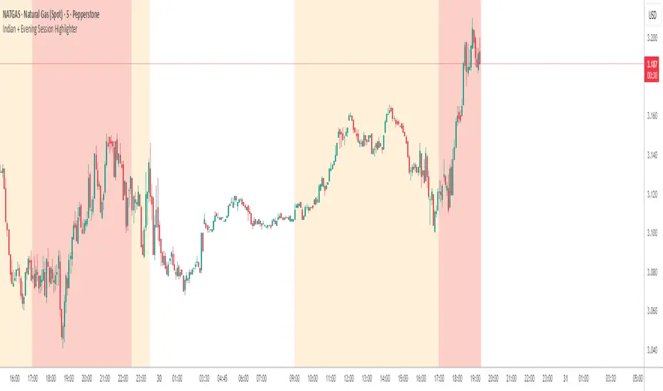
Indian + Evening Session HighlighterThis indicator visually highlights two key trading windows for Indian instruments according to IST:
Indian Session: 9:00 AM to 11:30 PM IST is shaded light orange on the chart, representing the main domestic trading hours for stocks, indices, commodities, or derivatives.
Evening Session: 5:00 PM to 10:30 PM IST is shaded light red, marking the commonly followed evening window, which often captures the impact of US and European market movements.
The indicator automatically overlays these session backgrounds on your chart, helping you quickly identify when price action occurs during India’s core and evening trade windows. This allows traders to focus on strategies specific to these time intervals, identify session-based volatility, and avoid trading during less active periods. If the evening session overlaps with the Indian session, the colors are layered for visual clarity.
It is ideal for intraday traders, option strategists, and anyone monitoring Indian market rhythms or US-linked volatility impacts on Indian assets. No inputs are required; simply apply the script and view distinct session highlights for improved timing and decision making.
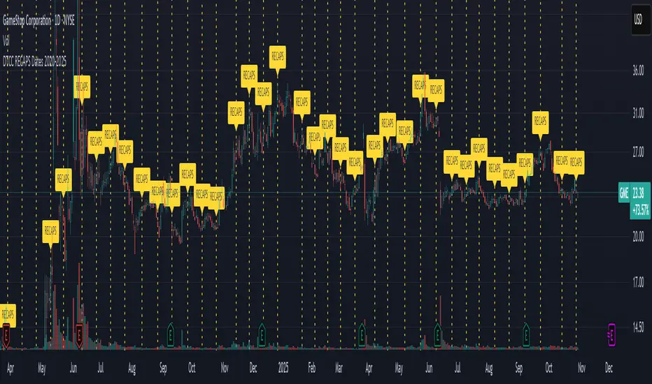
DTCC RECAPS Dates 2020-2025This is a simple indicator which marks the RECAPS dates of the DTCC, during the periods of 2020 to 2025.
These dates have marked clear settlement squeezes in the past, such as GME's squeeze of January 2021.
------------------------------------------------------------------------------------------------------------------
The Depository Trust & Clearing Corporation (DTCC) has published the 2025 schedule for its Reconfirmation and Re-pricing Service (RECAPS) through the National Securities Clearing Corporation (NSCC). RECAPS is a monthly process for comparing and re-pricing eligible equities, municipals, corporate bonds, and Unit Investment Trusts (UITs) that have aged two business days or more .
At its core, the Reconfirmation and Re-pricing Service (RECAPS) is a risk management tool used by the National Securities Clearing Corporation (NSCC), a subsidiary of the DTCC. Its primary purpose is to reduce the risks associated with aged, unsettled trades in the U.S. securities market .
When a trade is executed, it is sent to the NSCC for clearing and settlement. However, for various reasons, some trades may not settle on their scheduled date and become "aged." These unsettled trades create risk for both the trading parties and the clearinghouse (NSCC) because the value of the underlying securities can change over time. If a trade fails to settle and one of the parties defaults, the NSCC may have to step in to complete the transaction at the current market price, which could result in a loss.
RECAPS mitigates this risk by systematically re-pricing these aged, open trading obligations to the current market value. This process ensures that the financial obligations of the clearing members accurately reflect the present value of the securities, preventing the accumulation of significant, unmanaged market risk .
Detailed Mechanics: How Does it Work?
The RECAPS process revolves around two key dates you asked about: the RECAPS Date and the Settlement Date .
The RECAPS Date: On this day, the NSCC runs a process to identify all eligible trades that have remained unsettled for two business days or more. These "aged" trades are then re-priced to the current market value. This re-pricing is not just a simple recalculation; it generates new settlement instructions. The original, unsettled trade is effectively cancelled and replaced with a new one at the current market price. This is done through the NSCC's Obligation Warehouse.
The Settlement Date: This is typically the business day following the RECAPS date. On this date, the financial settlement of the re-priced trades occurs. The difference in value between the original trade price and the new, re-priced value is settled between the two trading parties. This "mark-to-market" adjustment is processed through the members' settlement accounts at the DTCC.
Essentially, the process ensures that any gains or losses due to price changes in the underlying security are realized and settled periodically, rather than being deferred until the trade is ultimately settled or cancelled.
Are These Dates Used to Check Margin Requirements?
Yes, indirectly, this process is closely tied to managing margin and collateral requirements for NSCC members. Here’s how:
The NSCC requires its members to post collateral to a clearing fund, which acts as a mutualized guarantee against defaults. The amount of collateral each member must provide is calculated based on their potential risk exposure to the clearinghouse.
By re-pricing aged trades to current market values through RECAPS, the NSCC gets a more accurate picture of each member's outstanding obligations and, therefore, their current risk profile. If a member has a large number of unsettled trades that have moved against them in value, the re-pricing will crystallize that loss, which will be settled the next day.
This regular re-pricing and settlement of aged trades prevent the build-up of large, unrealized losses that could increase a member's risk profile beyond what their posted collateral can cover. While RECAPS is not the only mechanism for calculating margin (the NSCC has a complex system for daily margin calls based on overall portfolio risk), it is a crucial component for managing the specific risk posed by aged, unsettled transactions. It ensures that the value of these obligations is kept current, which in turn helps ensure that collateral levels remain adequate.
--------------------------------------------------------------------------------------------------------------
Future dates of 2025:
- November 12, 2025 (Wed)
- November 25, 2025 (Tue)
- December 11, 2025 (Thu)
- December 29, 2025 (Mon)
The dates for 2026 haven't been published yet at this time.
The RECAPS process is essentially the industry's way of retrying the settlement of all unresolved FTDs, netting outstanding obligations, and gradually forcing resolution (either delivery or buy-in). Monitoring RECAPS cycles is one way to track the lifecycle, accumulation, and eventual resolution (or persistence) of failures to deliver in the U.S. market.
The US Stock market has become a game of settlement dates and FTDs, therefore this can be useful to track.
ProScalper📊 ProScalper - Professional 1-Minute Scalping System
🎯 Overview
ProScalper is a sophisticated, multi-confluence scalping indicator designed specifically for 1-minute chart trading. Combining advanced technical analysis with intelligent signal filtering, it provides high-probability trade setups with clear entry, stop loss, and take profit levels.
✨ Key Features
🔺 Smart Signal Detection
Range Filter Technology: Fast-responding trend detection (25-period) optimized for 1-minute timeframe
Medium-sized triangles appear above/below candles for clear buy/sell signals
Only most recent signal shown - no chart clutter
Automatically deletes old signals when new ones appear
📋 Real-Time Signal Table
Top-center display shows complete trade breakdown
Grade system: A+, A, B+, B, C+ ratings for every setup
All confluence reasons listed with checkmarks
Score and R:R displayed for instant trade quality assessment
Color-coded: Green for LONG, Red for SHORT
📐 Multi-Confluence Analysis
ProScalper combines 10+ technical factors:
✅ EMA Trend: 4 EMAs (200, 48, 13, 8) for multi-timeframe alignment
✅ VWAP: Dynamic support/resistance
✅ Fibonacci Retracement: Golden ratio (61.8%), 50%, 38.2%, 78.6%
✅ Range Filter: Adaptive trend confirmation
✅ Pivot Points: Smart reversal detection
✅ Volume Analysis: Spike detection and volume profile
✅ Higher Timeframe: 5-minute trend confirmation
✅ HTF Support/Resistance: Key levels from higher timeframes
✅ Liquidity Sweeps: Smart money detection
✅ Opening Range Breakout: First 15-minute range
💰 Complete Trade Management
Entry Lines: Dashed green (LONG) or red (SHORT) showing exact entry
Stop Loss: Red dashed line with price label
Take Profit: Blue dashed line with price label and R:R
Partial Exits: 1R level marked with orange dashed line
All lines extend 10 bars for clean alignment with Fibonacci levels
📊 Dynamic Risk/Reward
Adaptive R:R calculation based on market volatility
Targets adjusted for pivot distances
Minimum 1.2:1 to maximum 3.5:1 for scalping
Position sizing based on account risk percentage
🎨 Professional Visualization
Clean chart layout - no clutter, only essential information
Custom EMA colors: Red (200), Aqua (48), Green (13), White (8)
Gold VWAP line for key support/resistance
Color-coded Fibonacci: Bright yellow (61.8%), white (50%), orange (38.2%), fuchsia (78.6%)
No shaded zones - pure price action focus
📈 Performance Tracking
Real-time statistics table (optional)
Win rate, total trades, P&L tracking
Average R:R and win/loss ratios
Setup-specific performance metrics
⚙️ Settings & Customization
Risk Management
Adjustable account risk per trade (default: 0.5%)
ATR-based stop loss multiplier (default: 0.8 for tight scalping)
Dynamic position sizing
Signal Sensitivity
Confluence Score Threshold: 40-100 (default: 55 for balanced signals)
Range Filter Period: 25 bars (fast signals for 1-min)
Range Filter Multiplier: 2.2 (tighter bands for more signals)
Visual Controls
Toggle signal table on/off
Show/hide Fibonacci levels
Control EMA visibility
Adjust table text size
Partial Exits
1R: 50% (default)
2R: 30% (default)
3R: 20% (default)
Fully customizable percentages
Trailing Stops
ATR-Based (best for scalping)
Pivot-Based
EMA-Based
Breakeven trigger at 0.8R
🎯 Best Use Cases
Ideal For:
✅ 1-minute scalping on liquid instruments
✅ Day traders looking for quick 2-8 minute trades
✅ High-frequency trading with 8-15 signals per session
✅ Trending markets where Range Filter excels
✅ Crypto, Forex, Futures - works on all liquid assets
Trading Style:
Timeframe: 1-minute (can work on 3-5 min with adjusted settings)
Hold Time: 3-8 minutes average
Target: 1.2-3R per trade
Frequency: 8-15 signals per day
Win Rate: 45-55% (with proper risk management)
📋 How to Use
Step 1: Wait for Signal
Watch for green triangle (BUY) or red triangle (SELL)
Signal table appears at top center automatically
Step 2: Review Confluence
Check grade (prefer A+, A, B+ for best quality)
Review all reasons listed in table
Confirm score is above your threshold (55+ recommended)
Note the R:R ratio
Step 3: Enter Trade
Enter at current market price
Set stop loss at red dashed line
Set take profit at blue dashed line
Mark 1R level (orange line) for partial exit
Step 4: Manage Trade
Exit 50% at 1R (orange line)
Move to breakeven after 0.8R
Trail remaining position using your chosen method
Exit fully at TP or opposite signal
🎨 Chart Setup Recommendations
Optimal Display:
Timeframe: 1-minute
Chart Type: Candles or Heikin Ashi
Background: Dark theme for best color visibility
Volume: Enable volume bars below chart
Complementary Indicators (optional):
Order flow/Delta for institutional confirmation
Market profile for key levels
Economic calendar for news avoidance
⚠️ Important Notes
Risk Disclaimer:
Not financial advice - for educational purposes only
Always use proper risk management (0.5-1% per trade max)
Past performance doesn't guarantee future results
Test on demo account before live trading
Best Practices:
✅ Trade during high liquidity hours (9:30-11 AM, 2-4 PM EST)
✅ Avoid news events and market open/close (first/last 2 minutes)
✅ Use tight stops (0.8-1.0 ATR) for 1-minute scalping
✅ Take partial profits quickly (1R = 50% off)
✅ Respect max daily loss limits (3% recommended)
✅ Focus on A and B grade setups for consistency
What Makes This Different:
🎯 Complete system - not just signals, but full trade management
📊 Multi-confluence - 10+ factors analyzed per trade
🎨 Professional visualization - clean, focused chart design
⚡ Optimized for 1-min - settings specifically tuned for fast scalping
📋 Transparent reasoning - see exactly why each trade was taken
🏆 Grade system - instantly know trade quality
🔧 Technical Details
Pine Script Version: 5
Overlay: Yes (plots on price chart)
Max Lines: 500
Max Labels: 100
Non-repainting: All signals confirmed on bar close
Alerts: Compatible with TradingView alerts
📞 Support & Updates
This indicator is actively maintained and optimized for 1-minute scalping. Settings can be adjusted for different timeframes and trading styles, but default configuration is specifically tuned for high-frequency 1-minute scalping.
🚀 Get Started
Add ProScalper to your 1-minute chart
Adjust settings to your risk tolerance
Wait for signals (green/red triangles)
Follow the signal table guidance
Manage trades using provided levels
Track performance with stats table
Happy Scalping! 📊⚡💰

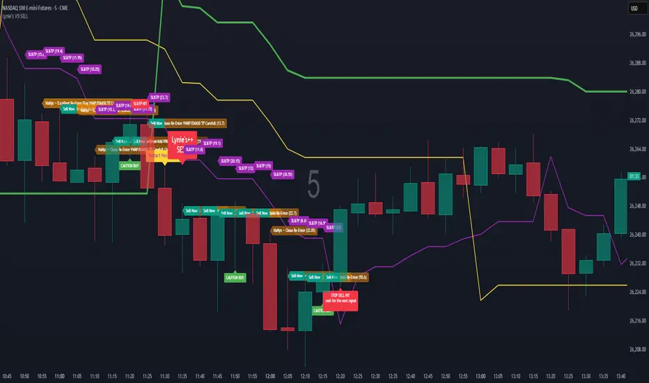
Lynie's V9 SELL🟢🔴 Lynie’s V8 — BUY & SELL (Mirrored, Interlocking System)
Lynie’s V8 is a paired long/short engine built as two mirrored scripts—Lynie’s V8 BUY and Lynie’s V8 SELL—that read price the same way, flip conditions symmetrically, and manage trades with the exact logic on opposite sides. Use either one standalone or run both together for full two-sided automation of entries, re-entries, caution states, and adaptive SL/TP.
✳️ What “mirrored” means here
Supertrend Tri-Stack (10/11/12):
BUY: ST10 primary pierce; ST12 fallback; “PAG Buy” when price pierces any ST while above the other two.
SELL: Exact inverse—ST10 primary pierce down; ST12 fallback; “PAG Sell” when price pierces any ST while below the other two.
Re-Enter Clusters:
BUY: Ratcheted up (Heikin-Ashi green holds/tightens).
SELL: Ratcheted down (Heikin-Ashi red holds/tightens).
Both sides use the same cluster age/decay math, care penalties, session awareness, and fast-candle tightening.
Care Flags (context risk):
Ichimoku, MACD, RSI combine into single and paired flags that tighten or widen offsets on both sides with the same scoring.
VWAP–EMA50 (5m) cluster gate:
Identical distance checks for BUY/SELL. When the mean cluster is present, offsets and labels adapt (tighter/“riskier scalp” messaging).
Golden Pocket A/B/C (prev-day):
Same fib boxes & labeling (gold tone) on both sides to call out TP-friendly zones.
SL/TP Envelope:
Shared dynamic engine: per-bar decay, fast-candle expansion, and care-based compress/relax—all mirrored for up/down.
Caution Labels:
BUY side prints CAUTION SELL if HA flips red inside an active long cluster.
SELL side prints CAUTION BUY if HA flips green inside an active short cluster.
Same latching & auto-release behavior.
🧠 Core workflow (both sides)
Primary trigger via ST10 pierce (structure shift) with an ST12 fallback when ST10 didn’t qualify.
PAG Mode when price is already on the right side of the other two STs—strongest conviction.
Cluster phase begins after a signal: ratcheted re-entry level, session-aware offsets, dynamic tightening on fast bars.
Care system shapes every re-entry & SL/TP label (Ichi/MACD/RSI combos + VWAP/EMA gate + QQE).
Protective layer: SL-wick and SL-body logic, caution flips, and “hold 1 bar” cluster carry after SL to avoid whipsaw spam.
🔎 Labels & messages (shared vocabulary)
Lynie’s / Lynie’s+ / Lynie’s++ — strength tiers (ST12 involvement & clean context).
Re-Enter / Excellent Re-Enter — cluster pullback quality; ratchet shows the “must-hold” zone.
SL&TP (n) — live offset multiplier the engine is using right now.
CAUTION BUY / CAUTION SELL — HA flip against the active side inside the cluster.
Restart Next Candle — visual cue to re-arm after a confirmed signal bar.
⚡ Why run both together
Continuity: When a long cycle ends (SL or caution degradation), the SELL engine is already tracking the inverse without re-tuning.
Symmetry: Same math, same signals, opposite direction—no hidden biases.
Coverage: Trend hand-offs are cleaner; you don’t miss early shorts after a long fade (and vice versa).
🔧 Recommended usage
Intraday futures (ES/NQ) or any liquid market.
Keep the VWAP–EMA cluster ON; it filters FOMO chases.
Honor Caution flips inside cluster—scale down or wait for the next clean re-enter.
Treat Golden Zones as TP magnets, not guaranteed reversals.
📌 Notes
Both scripts are Pine v6 and independent. Load BUY and SELL together for the full experience.
All offsets (re-enter & SL/TP) are visible in labels—so you always know why a zone is where it is.
Alerts are provided for signals, re-enter hits, caution, and SL events on both sides.
Summary: Lynie’s V8 BUY & SELL are vice-versa twins—one framework, two directions—delivering consistent entries, adaptive re-entries, and contextual risk management whether the market is pressing up or breaking down.
Broad Market for Crypto + index# Broad Market Indicator for Crypto
## Overview
The Broad Market Indicator for Crypto helps traders assess the strength and divergence of individual cryptocurrency assets relative to the overall market. By comparing price deviations across multiple assets, this indicator reveals whether a specific coin is moving in sync with or diverging from the broader crypto market trend.
## How It Works
This indicator calculates percentage deviations from simple moving averages (SMA) for both individual assets and an equal-weighted market index. The core methodology:
1. **Deviation Calculation**: For each asset, the indicator measures how far the current price has moved from its SMA over a specified lookback period (default: 24 hours). The deviation is expressed as a percentage: `(Current Price - SMA) / SMA × 100`
2. **Market Index Construction**: An equal-weighted index is built from selected cryptocurrencies (up to 15 assets). The default composition includes major crypto assets: BTC, ETH, BNB, SOL, XRP, ADA, AVAX, LINK, DOGE, and TRX.
3. **Comparative Analysis**: The indicator displays both the current instrument's deviation and the market index deviation on the same panel, making it easy to spot relative strength or weakness.
## Key Features
- **Customizable Asset Selection**: Choose up to 15 different cryptocurrencies to include in your market index
- **Flexible Configuration**: Toggle individual assets on/off for display and index calculation
- **Current Instrument Tracking**: Automatically plots the deviation of whatever chart you're viewing
- **Visual Clarity**: Color-coded lines for easy differentiation between assets, with the market index shown as a filled area
- **Adjustable Lookback Period**: Modify the SMA period to match your trading timeframe
## How to Use
### Identifying Market Divergences
- When the current instrument deviates significantly above the index, it shows relative strength
- When it deviates below, it indicates relative weakness
- Assets clustering around zero suggest neutral market conditions
### Trend Confirmation
- If both the index and your asset are rising together (positive deviation), it confirms a broad market uptrend
- Divergence between asset and index can signal unique fundamental factors or early trend changes
### Entry/Exit Signals
- Extreme deviations from the index may indicate overbought/oversold conditions relative to the market
- Convergence back toward the index line can signal mean reversion opportunities
## Settings
- **Lookback Period**: Adjust the SMA calculation period (default: 24 hours)
- **Asset Configuration**: Select which cryptocurrencies to monitor and include in the index
- **Display Options**: Show/hide individual assets, current instrument, and market index
- **Color Customization**: Personalize colors for better visual analysis
## Best Practices
- Use on higher timeframes (4H, Daily) for more reliable signals
- Combine with volume analysis for confirmation
- Consider fundamental news when assets show extreme divergence
- Adjust the asset basket to match your trading focus (DeFi, L1s, memecoins, etc.)
## Technical Notes
- The indicator uses `request.security()` to fetch data from multiple symbols
- Deviations are calculated independently for each asset
- The zero line represents perfect alignment with the moving average
- Index calculation automatically adjusts based on active assets
## Default Assets
1. BTC (Bitcoin) - BINANCE:BTCUSDT
2. ETH (Ethereum) - BINANCE:ETHUSDT
3. BNB (Binance Coin) - BINANCE:BNBUSDT
4. SOL (Solana) - BINANCE:SOLUSDT
5. XRP (Ripple) - BINANCE:XRPUSDT
6. ADA (Cardano) - BINANCE:ADAUSDT
7. AVAX (Avalanche) - BINANCE:AVAXUSDT
8. LINK (Chainlink) - BINANCE:LINKUSDT
9. DOGE (Dogecoin) - BINANCE:DOGEUSDT
10. TRX (Tron) - BINANCE:TRXUSDT
Additional slots (11-15) are available for custom asset selection.
---
This indicator is particularly useful for cryptocurrency traders seeking to understand market breadth and identify opportunities where specific assets are diverging from overall market sentiment.

Crypto Index Price# Crypto Index Price - Indicator Description
## 📊 What is this indicator?
**Crypto Index Price** is an indicator for creating your own cryptocurrency index based on an equal-weighted portfolio. It allows you to track the overall dynamics of the cryptocurrency market through a composite index of selected assets.
## 🎯 Key Features
- **Up to 20 assets in the index** — create an index from any trading pairs
- **Equal-weighted methodology** — each asset has the same weight in the index
- **Moving average** — optional trend filter for the index
- **Flexible visualization settings** — customizable colors and line thickness
## 📈 How to Use
The indicator is displayed in a separate pane below the chart and shows:
1. **Blue line** — crypto index value
2. **Orange line** (optional) — moving average of the index
### Trading Applications:
- **Identify overall market trend** — if the index is rising, most coins are in an uptrend
- **Divergences** — divergence between your asset and the index may signal local opportunities
- **Signal confirmation** — use the index to confirm trading decisions on individual coins
- **Market condition filter** — trade longs when index is above MA, shorts when below
## ⚙️ Settings
### Assets (Symbols)
- **Asset 1-10** — main cryptocurrencies (default: BTC, ETH, BNB, SOL, XRP, ADA, AVAX, LINK, DOGE, TRX)
- **Asset 11-20** — additional slots for index expansion
### Visual Parameters
- **Index line color** — main line color (default: blue)
- **Line width** — from 1 to 5 pixels
- **Show moving average** — enable/disable MA
- **MA period** — moving average calculation period (default: 20)
- **MA color** — moving average line color (default: orange)
## 💡 Recommendations
- For a top coins index, use 5-10 largest cryptocurrencies by market cap
- For an altcoin index, add medium and small coins from your sector
- Use MA to filter false signals and identify the global trend
- Compare individual asset behavior with the index to find anomalies
## ⚠️ Important
The indicator uses equal-weighted methodology — each coin contributes equally regardless of price or market cap. This differs from cap-weighted indices and may provide a different market perspective.
---
*This indicator is intended for analysis and is not trading advice. Always conduct your own analysis before making trading decisions.*
---

Liquidity Sniper V3 (ANTI-FAKEOUT)An advanced institutional trading indicator combining liquidity pool targeting, smart money concepts, and momentum-based entries with comprehensive risk management.
🎯 CORE FEATURES:
- Liquidity Sniper Module: Identifies and targets major liquidity pools (PDH/PDL, PWH/PWL, Equal Highs/Lows, HVN/LVN edges)
- Anti-Fakeout Stack: 10-layer confirmation system including VWAP reclaim, micro BOS, displacement, relative volume, and mitigation entries
- Momentum Engulf Add-On: Catches high-velocity impulsive moves with engulfing candles, volume spikes, and volatility breakouts
- GARCH Volatility Filter: Dynamic volatility analysis to avoid choppy conditions
- Multi-Timeframe Confirmation: Ensures alignment across timeframes before entries
📊 SIGNAL CLASSIFICATION:
- BEST (Green): Highest probability setups with all confirmations aligned - 6.0+ score
- BETTER (Medium Green): Strong setups with most confirmations - 4.5-6.0 score
- GOOD (Light Green): Valid setups with basic confirmations - 3.0-4.5 score
🔍 TRADE SCENARIOS:
S1: Liquidity Reversal - Sweeps + reversals at key levels with displacement
S2: Continuation - Trend following with VWAP mean reversion
S3: Mean Reversion - Extreme deviations (2σ+) with Fibonacci exhaustion
S4: Deep Sweep - 3σ sweeps at major liquidity with high confluence
⚡ MOMENTUM TRIGGERS:
- MET (Momentum Engulf): Bullish/bearish engulfing with 1.5x+ volume spike and ATR impulse
- VBT (Volatility Breakout): Range breakouts with sigma bursts and participation
🛡️ RISK MANAGEMENT:
- Dynamic TP/SL based on ATR, VWAP bands, and liquidity pools
- 3-tier targets (T1: VWAP, T2: Nearest pool, T3: 5R extension)
- Early invalidation tracking (0.5R movement monitoring)
- Minimum 2:1 RR requirement with cooldown periods
- RTH session filters and anti-spam protection
📈 TECHNICAL EDGE:
- SMT Divergence detection vs ES correlation
- CVD (Cumulative Volume Delta) divergence confirmation
- FVG (Fair Value Gap) and Order Block mitigation entries
- Equal highs/lows clustering analysis
- Volume profile HVN/LVN identification
⚙️ FULLY CUSTOMIZABLE:
All parameters adjustable including cooldowns, proximity thresholds, ATR multipliers, RR floors, and scenario weights.
Perfect for: ES/NQ futures, forex majors, and liquid stocks. Works on 1-15 min timeframes. Best results during NY session (9:35-11:00 AM & 1:30-3:30 PM ET).
Created for serious traders seeking institutional-grade edge with quantifiable risk/reward and high-probability setups

FX Sessions by m_cptForex Intraday Sessions Indicator, config time in UTC-4. Support 4 main sessions, smooth end-to-start candles mode, without gaps if your sessions has config like:
1) 19:00 - 03:00
2) 02:00 - 03:00
3) 03:00 -11:00
No excluded last candles issue on all TFs.
Working on LTF up to 1h TF since its intraday sessions indicator.

Previous session High/Low – Asia London USA Overview
This indicator automatically plots the Previous Day’s (PD) session Highs and Lows for the Asia (Tokyo), London, and USA (New York) trading sessions.
Each session is color-coded for clarity:
🟩 Asia (Green)
🟥 London (Red)
🟦 USA (Blue)
At the close of each session, the indicator records that session’s high and low, draws horizontal lines across the chart, and labels them neatly in the center of each range — above the high and below the low for perfect visual balance.
⚙️ How It Works
The script continuously tracks the current high and low within each session.
When a session closes, those values are locked in as the PD High and PD Low.
Clean lines and centered labels are drawn immediately.
The labels automatically offset slightly above or below the line to avoid overlap, with user-controlled spacing.
This helps traders quickly identify where price interacts with the previous session’s structure, a core concept for many session-based and liquidity-based strategies.
🧭 Sessions and Timezones
Each market session runs in its native timezone, so you can align them perfectly to your chart or your preferred trading hours:
Asia Session: Default 08:30 – 11:00 (Australia/Adelaide time)
London Session: Default 08:00 – 10:00 (Europe/London)
USA Session: Default 09:30 – 16:00 (America/New_York)
You can change each session’s hours and timezone from the Inputs panel.
🎨 Customization
In the Inputs menu you can:
Toggle each session on or off
Choose line color and thickness
Enable or disable labels
Adjust vertical offset (ticks) for label spacing
“High label offset” – moves label further above the high line
“Low label offset” – moves label further below the low line
These adjustments make it easy to keep charts clean and readable on any instrument or timeframe.
📈 Practical Use
This indicator is ideal for:
Session traders who mark PD Highs/Lows as liquidity zones
London or NY session scalpers who watch for breakouts, fakeouts, or reversals
ICT / Smart Money Concepts users wanting automatic session reference levels
Anyone wanting a quick visual map of inter-session structure

Asia & London Session High/Low – EOD Segments (v4.5)What it does
Plots the Asia and London session high & low each day.
When a session ends, its high/low are locked (non-repainting) and drawn as horizontal segments that auto-extend to the end of that same day (no infinite rays).
Optional labels show the exact level at session close.
Toggle whether to keep prior days on the chart or auto-clear them on the first bar of a new day.
Why traders use it
Quickly see overnight liquidity levels that often act as magnets or barriers during the U.S. session.
Map session range extremes for breakout/reversal planning, partials, and invalidation.
Works great alongside VWAP, 8/20/200 MAs, or your NY session tools to build confluence.
How it works
You define the session windows (defaults: Asia 00:00–06:00, London 07:00–11:00).
While a session is active, the script tracks running high/low.
On the bar after the session ends, the level is finalized and drawn; the segment’s right edge updates each bar until EOD, then stops automatically.
Inputs
Session Timezone: “Exchange”, UTC, or a specific region (set this to match your venue).
Asia / London Session: editable HHMM-HHMM windows.
Show Asia / Show London: enable either/both sessions.
Keep history: keep or auto-delete previous days.
Show labels: price labels at session close.
Colors & width: customize high/low colors and line width.
Best practices
Use on intraday timeframes (1–60m).
For equities/futures, set timezone to your exchange (e.g., America/New_York). For FX/crypto, pick what matches your workflow.
Common tweak: London 08:00–12:00 local; Asia 00:00–05:00 or your broker’s definition.
Notes
Non-repainting: levels only print once the session is complete.
Designed to be light and reliable—no boxes, just clean lines and labels.
If you want NY session levels, midlines (50%), anchored stop-time, or alerts on touches, this script can be extended.
For educational use only. Not financial advice.

ICT Liquidity Sweep Asia/London 1 Trade per High & Low🧠 ICT Liquidity Sweep Asia/London — 1 Trade per High & Low
This strategy is inspired by the ICT (Inner Circle Trader) concepts of liquidity sweeps and market structure, focusing on the Asia and London sessions.
It automatically identifies liquidity grabs (sweeps) above or below key session highs/lows and enters trades with a fixed risk/reward ratio (RR).
----------------------------------------------------------------------------------
----------------------------------------------------------------------------------
⚙️ Core Logic
-Asia Session: 8:00 PM – 11:59 PM (New York time)
-London Session: 2:00 AM – 5:00 AM (New York time)
-The script marks the Asia High/Low and London High/Low ranges for each day.
-When the market sweeps above a session high → potential Short setup
-When the market sweeps below a session low → potential Long setup
-A trade is triggered when the confirmation candle closes in the opposite direction of the sweep (bearish after a high sweep, bullish after a low sweep).
-Only one trade per sweep type (1 per High, 1 per Low) is allowed per session.
----------------------------------------------------------------------------------
----------------------------------------------------------------------------------
📈 Risk Management
-Configurable Risk/Reward Target (default = 2:1)
-Configurable Position Size (number of contracts)
-Each trade uses a fixed Stop Loss (beyond the wick of the sweep) and a Take Profit calculated from the RR setting.
-All trades are automatically logged in the Strategy Tester with performance metrics.
----------------------------------------------------------------------------------
----------------------------------------------------------------------------------
💡 Features
✅ Visual session highlighting (Asia = Aqua, London = Orange)
✅ Automatic liquidity line plotting (session highs/lows)
✅ Entry & exit labels (optional visual display)
✅ Customizable RR and contract size
✅ Works on any instrument (ideal for indices, futures, or forex)
✅ Compatible with all timeframes (optimized for 1M–15M)
----------------------------------------------------------------------------------
----------------------------------------------------------------------------------
⚠️ Notes
-Best used on New York time-based charts.
-Designed for educational and backtesting purposes — not financial advice.
-Use as a foundation for further optimization (e.g., SMT confirmation, FVG filter, or time-based restrictions).
----------------------------------------------------------------------------------
----------------------------------------------------------------------------------
🧩 Recommended Use
Pair this with:
-ICT’s concepts like CISD (Change in State of Delivery) and FVGs (Fair Value Gaps)
-Higher timeframe liquidity maps
-Session bias or daily narrative filters
----------------------------------------------------------------------------------
----------------------------------------------------------------------------------
Author: jygirouard
Strategy Version: 1.3
Type: ICT Liquidity Sweep Automation
Timezone: America/New_York
Smart Money Dynamics Blocks - Pearson MatrixSmart Money Dynamics Blocks — Pearson Matrix
A structural fusion of Prime Number Theory, Pearson Correlation, and Cumulative Delta Geometry.
1. Mathematical Foundation
This indicator is built on the intersection of Prime Number Theory and the Pearson correlation coefficient, creating a structural framework that quantifies how price and time evolve together.
Prime numbers — unique, indivisible, and irregular — are used here as nonlinear time intervals. Each prime length (2, 3, 5, 7, 11…97) represents a regression horizon where correlation is measured between price and time. The result is a multi-scale correlation lattice — a geometric matrix that captures hidden directional strength and temporal bias beyond traditional moving averages.
2. The Pearson Matrix Logic
For every prime interval p, the indicator calculates the linear correlation:
r_p = corr(price, bar_index, p)
Each r_p reflects how closely price and time move together across a prime-defined window. All r_p values are then averaged to create avgR, a single adaptive coefficient summarizing overall structural coherence.
- When avgR > 0.8 → strong positive correlation (labeled R+).
- When avgR < -0.8 → strong negative correlation (labeled R−).
This approach gives a mathematically grounded definition of trend — one that isn’t based on pattern recognition, but on measurable correlation strength.
3. Sequential Prime Slope and Median Pivot
Using the ordered sequence of 25 prime intervals, the model computes sequential slopes between adjacent primes. These slopes represent the rate of change of structure between two prime scales. A robust median aggregator smooths the slopes, producing a clean, stable directional vector.
The system anchors this slope to the 41-bar pivot — the median of the first 25 primes — serving as the geometric midpoint of the prime lattice. The resulting yellow line on the chart is not an ordinary regression line; it’s a dynamic prime-slope function, adapting continuously with correlation feedback.
4. Regression-Style Parallel Bands
Around this prime-slope line, the indicator constructs parallel bands using standard deviation envelopes — conceptually similar to a regression channel but recalculated through the prime–Pearson matrix.
These bands adjust dynamically to:
- Volatility, via standard deviation of residuals.
- Correlation strength, via avgR sign weighting.
Together, they visualize statistical deviation geometry, making it easier to observe symmetry, expansion, and contraction phases of price structure.
5. Volume and Cumulative Delta Peaks
Below the geometric layer, the indicator incorporates a custom lower-timeframe volume feed — by default using 15-second data (custom_tf_input_volume = “15S”). This allows precise delta computation between up-volume and down-volume even on higher timeframe charts.
From this feed, the indicator accumulates delta over a configurable period (default: 100 bars). When cumulative delta reaches a local maximum or minimum, peak and trough markers appear, showing the precise bar where buying or selling pressure statistically peaked.
This combination of geometry and order flow reveals the intersection of market structure and energy — where liquidity pressure expresses itself through mathematical form.
6. Chart Interpretation
The primary chart view represents the live execution of the indicator. It displays the relationship between structural correlation and volume behavior in real time.
Orange “R+” and blue “R−” labels indicate regions of strong positive or negative Pearson correlation across the prime matrix. The yellow median prime-slope line serves as the structural backbone of the indicator, while green and red parallel bands act as dynamic regression boundaries derived from the underlying correlation strength. Peaks and troughs in cumulative delta — displayed as numerical annotations — mark statistically significant shifts in buying and selling pressure.
The secondary visualization (Prime Regression Concept) expands on this by illustrating how regression behavior evolves across prime intervals. Each colored regression fan corresponds to a prime number window (2, 3, 5, 7, …, 97), demonstrating how multiple regression lines would appear if drawn independently. The indicator integrates these into one unified geometric model — eliminating the need to plot tens of regression lines manually. It’s a conceptual tool to help visualize the internal logic: the synthesis of many small-scale regressions into a single coherent structure.
7. Interpretive Insight
This model is not a prediction tool; it’s an instrument of mathematical observation. By translating price dynamics into a prime-structured correlation space, it reveals how coherence unfolds through time — not as a forecast, but as a measurable evolution of structure.
It unifies three analytical domains:
- Prime distribution — defines a nonlinear temporal architecture.
- Pearson correlation — quantifies statistical cohesion.
- Cumulative delta — expresses behavioral imbalance in order flow.
The synthesis creates a geometric analysis of liquidity and time — where structure meets energy, and where the invisible rhythm of market flow becomes measurable.
8. Contribution & Feedback
Share your observations in the comments:
- The time gap and alternation between R+ and R− clusters.
- How different timeframes change delta sensitivity or reveal compression/expansion.
- Prime intervals/clusters that tend to sit near turning points or liquidity shifts.
- How avgR behaves across assets or regimes (trending, ranging, high-vol).
- Notable interactions with the parallel bands (touches, breaks, mean-revert).
Your field notes help others read the model more effectively and compare contexts.
Summary
- Primes define the structure.
- Pearson quantifies coherence.
- Slope median stabilizes geometry.
- Regression bands visualize deviation.
- Cumulative delta locates imbalance.
Together, they construct a framework where mathematics meets market behavior.

NY Session Range Box with Labeled Time MarkersShows opening time ny session by timing with lines to inform traders to avoid 11:30am to 1:30pm for choppy sessions and mark early and power hour .

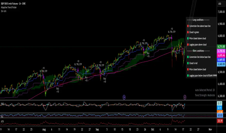
1hr ichi v6Ichimoku adapted to a 1hr chart
Set margin for positions to "0"
Adjust the number of contracts to the maximum drawdown you will accept. I use 11-13%
TASC 2025.11 The Points and Line Chart█ OVERVIEW
This script implements the Points and Line Chart described by Mohamed Ashraf Mahfouz and Mohamed Meregy in the November 2025 edition of the TASC Traders' Tips , "Efficient Display of Irregular Time Series”. This novel chart type interprets regular time series chart data to create an irregular time series chart.
█ CONCEPTS
When formatting data for display on a price chart, there are two main categorizations of chart types: regular time series (RTS) and irregular time series (ITS).
RTS charts, such as a typical candlestick chart, collect data over a specified amount of time and display it at one point. A one-minute candle, for example, represents the entirety of price movements within the minute that it represents.
ITS charts display data only after certain conditions are met. Since they do not plot at a consistent time period, they are called “irregular”.
Typically, ITS charts, such as Point and Figure (P&F) and Renko charts, focus on price change, plotting only when a certain threshold of change occurs.
The Points and Line (P&L) chart operates similarly to a P&F chart, using price change to determine when to plot points. However, instead of plotting the price in points, the P&L chart (by default) plots the closing price from RTS data. In other words, the P&L chart plots its points at the actual RTS close, as opposed to (price) intervals based on point size. This approach creates an ITS while still maintaining a reference to the RTS data, allowing us to gain a better understanding of time while consolidating the chart into an ITS format.
█ USAGE
Because the P&L chart forms bars based on price action instead of time, it displays displays significantly more history than a typical RTS chart. With this view, we are able to more easily spot support and resistance levels, which we could use when looking to place trades.
In the chart below, we can see over 13 years of data consolidated into one single view.
To view specific chart details, hover over each point of the chart to see a list of information.
In addition to providing a compact view of price movement over larger periods, this new chart type helps make classic chart patterns easier to interpret. When considering breakouts, the closing price provides a clearer representation of the actual breakout, as opposed to point size plots which are limited.
Because P&L is a new charting type, this script still requires a standard RTS chart for proper calculations. However, the main price chart is not intended for interpretation alongside the P&L chart; users can hide the main price series to keep the chart clean.
█ DISPLAYS
This indicator creates two displays: the "Price Display" and the "Data Display".
With the "Price display" setting, users can choose between showing a line or OHLC candles for the P&L drawing. The line display shows the close price of the P&L chart. In the candle display, the close price remains the same, while the open, high, and low values depend on the price action between points.
With the "Data display" setting, users can enable the display of a histogram that shows either the total volume or days/bars between the points in the P&L chart. For example, a reading of 12 days would indicate that the time since the last point was 12 days.
Note: The "Days" setting actually shows the number of chart bars elapsed between P&L points. The displayed value represents days only if the chart uses the "1D" timeframe.
The "Overlay P&L on chart" input controls whether the P&L line or candles appear on the main chart pane or in a separate pane.
Users can deactivate either display by selecting "None" from the corresponding input.
Technical Note: Due to drawing limitations, this indicator has the following display limits:
The line display can show data to 10,000 P&L points.
The candle display and tooltips show data for up to 500 points.
The histograms show data for up to 3,333 points.
█ INPUTS
Reversal Amount: The number of points/steps required to determine a reversal.
Scale size Method: The method used to filter price movements. By default, the P&L chart uses the same scaling method as the P&F chart. Optionally, this scaling method can be changed to use ATR or Percent.
P&L Method: The prices to plot and use for filtering:
“Close” plots the closing price and uses it to determine movements.
“High/Low” uses the high price on upside moves and low price on downside moves.
"Point Size" uses the closing price for filtration, but locks the price to plot at point size intervals.
ICT Killzones & MacrosICT Killzones & Macros (v1.1.5) — configurable ICT session windows + refined “macro” windows with live High/Low levels, optional extensions, next-window previews, and lightweight opening-price lines. Built to be clock-robust, timezone-aware, and performant on intraday charts.
Tip: All times are interpreted in your chosen IANA timezone (default: America/New_York) and auto-handle DST. You can rename, recolor, enable/disable, and retime every window.
What it plots
- Killzones (5) : Asia (19:00–02:00), London (02:00–05:00), NY AM (07:00–09:30), London Close (10:00–12:00), NY PM (13:30–16:00) — full-height boxes with optional header.
- Macros (8) (defaults tailored for common ICT “refined” windows): Asia-1 (18:00–21:00), Asia-2 (21:00–00:00), London-1 (01:00–04:00), AM-1 (09:45–10:15), AM-2 (10:45–11:15), Lunch (12:00–13:00), PM-1 (13:30–14:30), Power Hour (15:10–16:00).
- Live High/Low lines for the current Macro/Killzone window.
- Optional HL extension to the right until price crosses or the trading day rolls (style selectable).
- “Next” previews : earliest upcoming Macro and Killzone header; optional next-window background band.
- Opening Prices (3 lightweight time lines) : defaults 00:00, 08:30, 09:30 with right-edge labels, scoped to a session you choose (auto-cleans at session end).
- Key inputs & styling
- General : Timezone (IANA), “Sessions to show” (per window) to keep only the last N completed windows.
- Header : height (ticks), gap (ticks), fill opacity, border width/style, text size/color, toggle “Next Macro/Killzone” headers.
- Boxes : global fill opacity, global border width/style (used by both Macros & Killzones).
- High/Low : show HL, HL line style, extend on/off + extension style, optional extension labels.
- Opening Prices : enable Time 1/2/3, set HH:MM for each, session window, per-line colors, style (dotted/dashed/solid), width.
- Per-window controls : each Macro/Killzone has Enable, Session (HHMM-HHMM), Label, Fill color.
How to use (quick start)
- Set Timezone to your preference (default America/New_York).
- Toggle on the Macros and Killzones you trade. Adjust session times if needed.
- (Optional) Turn on Extend High/Low to project levels until crossed/day-roll.
- (Optional) Enable Next… headers to see the next upcoming window at a glance.
- (Optional) Configure Opening Prices (00:00 / 08:30 / 09:30 by default) and the session over which they appear.
Behavior & notes
- Time windows are computed by clock, not by guessing bar timestamps, making them robust across brokers and timeframes.
- With HL extension on, the current window’s levels extend until crossed or the end of the trading day (in your timezone). With it off, completed windows keep static HL markers (limited by “Sessions to show”).
- “Sessions to show” applies per Macro/Killzone to automatically prune older windows and keep charts snappy.
- Opening-price lines exist only within the chosen “Opening Prices Session” and are removed when it ends (keeps charts clean).
Defaults (color cues)
Killzones: Asia (blue), London (purple), NY AM (green), London Close (yellow), NY PM (orange).
Macros: neutral greys with Lunch and PM accents out of the box (all customizable).
Performance tips
- Reduce “Sessions to show” if you scroll far back in history.
- Disable “Next…” previews and/or extension labels on very slow machines.
- Narrow the “Opening Prices Session” window to exactly when you need those lines.
Changelog highlights
- v1.1.5 : Internal refinements and stability.
- v1.1.3 : Live High/Low lines for current windows + optional extension.
- v1.1.2 : Added “next Killzone” preview (to match “next Macro”).
- v1.1.0 : Defaults updated (5 KZ, 8 Macros). Removed “snap-to-killzone” behavior.
- v1.0.0 : Independent Macro vs. Killzone rendering; cleaner header logic.
- Known limitations
If your chart warns about drawings, trim “Sessions to show”.
If your broker session times differ from NY hours, adjust the sessions or change the indicator timezone.
Credits & intent
Inspired by ICT timing concepts; provided for education/mark-up, not financial advice.
Built to be flexible so you can mirror your personal playbook and journaling workflow.

Bollinger Band Screener [Pineify]Multi-Symbol Bollinger Band Screener Pineify – Advanced Multi-Timeframe Market Analysis
Unlock the power of rapid, multi-asset scanning with this original TradingView Pine Script. Expose trends, volatility, and reversals across your favorite tickers—all in a single, customizable dashboard.
Key Features
Screens up to 8 symbols simultaneously with individual controls.
Covers 4 distinct timeframes per symbol for robust, multi-timeframe analysis.
Integrates advanced Bollinger Band logic, adaptable with 11+ moving average types (SMA, EMA, RMA, HMA, WMA, VWMA, TMA, VAR, WWMA, ZLEMA, and TSF).
Visualizes precise state changes: Open/Parallel Uptrends & Downtrends, Consolidation, Breakouts, and more.
Highly interactive table view for instant signal interpretation and actionable alerts.
Flexible to any market: crypto, stocks, forex, indices, and commodities.
How It Works
For each chosen symbol and timeframe, the script calculates Bollinger Bands using your specified source, length, standard deviation, and moving average method.
Real-time state recognition assigns one of several states (Open Rising, Open Falling, Parallel Rising, Parallel Falling), painting the table with unique color codes.
State detection is rigorously defined: e.g., “Open Rising” is set when both bands and the basis rise, indicating strong up momentum.
All bands, signals, and strategies dynamically update as new bars print or user inputs change.
Trading Ideas and Insights
Identify volatility expansions and compressions instantly, spotting breakouts and breakdowns before they play out.
Spot multi-timeframe confluences—when trends align across several TFs, conviction increases for potential trades.
Trade reversals or continuations based on unique Bollinger Band patterns, such as squeeze-break or persistent parallel moves.
Harness this tool for scalping, swing trading, or systematic portfolio screens—your logic, your edge!
How Multiple Indicators Work Together
This screener’s core strength is its integration of multiple moving average types into Bollinger Band construction, not just standard SMA. Each average adapts the bands’ responsiveness to trend and noise, so traders can select the underlying logic that matches their market environment (e.g., HMA for fast moves or ZLEMA for smoothed lag). Overlaying 4 timeframes per symbol ensures trends, reversals, and volatility shifts never slip past your radar. When all MAs and bands synchronize across symbols and TFs, it becomes easy to separate real opportunity from market noise.
Unique Aspects
Perhaps the most flexible Bollinger Band screener for TradingView—choose from over 10 moving average methods.
Powerful multi-timeframe and multi-asset design, rare among Pine scripts.
Immediate visual clarity with color-coded table cells indicating band state—no need for guesswork or chart clutter.
Custom configuration for each asset and time slice to suit any trading style.
How to Use
Add the script to your TradingView chart.
Use the user-friendly input settings to specify up to 8 symbols and 4 timeframes each.
Customize the Bollinger Band parameters: source (price type), band length, standard deviation, and type of moving average.
Interpret the dashboard: Color codes and “state” abbreviations show you instantly which symbols and timeframes are trending, consolidating, or breaking out.
Take trades according to your strategy, using the screener as a confirmation or primary scan tool.
Customization
Fully customize: symbols, timeframes, source, band length, standard deviation multiplier, and moving average type.
Supports intricate watchlists—anything TradingView allows, this script tracks.
Adapt for cryptos, equities, forex, or derivatives by changing symbol inputs.
Conclusion
The Multi-Symbol Bollinger Band Screener “Pineify” is a comprehensive, SEO-optimized Pine Script tool to supercharge your market scanning, trend spotting, and decision-making on TradingView. Whether you trade crypto, stocks, or forex—its fast, intuitive, multi-timeframe dashboard gives you the informational edge to stay ahead of the market.
Try it now to streamline your trading workflow and see all the bands, all the trends, all the time!

Mean Reverting Suite [OmegaTools]Overview
The Mean Reverting Suits (MR Suite) by OmegaTools is an advanced analytical and visualization framework designed to identify directional exhaustion, statistical overextensions, and conditions consistent with mean-reversion dynamics. It integrates three pillars into a single display: a composite momentum-normalized oscillator, a percentile-based extension model with volume contextualization, and a dynamic structural mapping engine built on confirmed pivots. The indicator does not generate signals or prescribe trade actions; it provides objective context so users can evaluate market balance and the likelihood that price is departing from its recent statistical baseline.
Core logic
The composite oscillator blends MFI on two horizons and RSI on HL2, then averages them to produce a stabilized mean-reversion gauge. Candle and bar colors are mapped by a dual gradient centered at 50. Readings above 50 progressively shift from neutral gray toward the bearish accent color to reflect increasing momentum saturation; readings below 50 shift from the bullish accent color toward gray to reflect potential accumulation or temporary undervaluation. This continuous mapping avoids rigid thresholds and conveys the strength and decay of momentum as a smooth spectrum.
The percentile-based extension model measures the persistence of directional bias by tracking how many bars have elapsed since the last opposing condition. These rolling counts are compared to the 80th percentile of their own historical distributions stored in arrays. When a current streak exceeds its respective percentile, the environment is labeled as statistically extended in that direction. Background shading communicates this information and is modulated by relative volume, computed as live volume divided by a blended average of SMA(30) and EMA(11). Higher opacity implies greater liquidity participation during the extension.
The structural mapping module uses confirmed pivot highs and lows at the chosen length to create persistent horizontal levels that extend forward and automatically maintain themselves until price invalidates or refreshes them. These levels represent market memory zones and assist in reading where reactions previously formed. The engine updates in real time, ensuring the framework continuously reflects the prevailing structure.
Standard deviation and z-score overlay
The updated version introduces a mean and dispersion layer. A simple moving average of HL2 over twice the length provides the reference mean. Dispersion is estimated as the moving average of the absolute deviation between close and the mean over five times the length. The z-score is computed as the distance of price from the mean divided by this dispersion proxy. Visual arrows highlight observations where the absolute z-score exceeds two standard deviations, offering a concise view of statistically unusual departures from the local mean. This layer complements the percentile extension model by adding an orthogonal measure of extremity based on distributional distance rather than run length.
Visualization
Candle bodies and borders inherit the oscillator’s gradient color, creating an immediate sense of directional pressure and potential momentum fatigue. The chart background activates when the extension model detects a statistically rare streak, using blue tones for bearish extension and red tones for bullish extension, with intensity scaling by relative volume. Horizontal lines denote active pivot-based levels, automatically extending, truncating, and refreshing as structure evolves. The z-score arrows appear only when deviations exceed the ±2 threshold, keeping the display focused on noteworthy statistical events.
Inputs and configuration
Length controls the sensitivity of all modules. Lower values make the oscillator and pivot detection more reactive; higher values smooth readings and widen structural context. Bullish and Bearish colors are user-selectable to match platform themes or accessibility requirements.
Interpretation guidance
A strong red background indicates an unusually extended bullish run in the presence of meaningful volume; a strong blue background indicates an unusually extended bearish run in the presence of meaningful volume. Candle gradients near deep bearish tones suggest oscillator readings well above 50; gradients near deep bullish tones suggest oscillator readings well below 50. Pivot lines mark the most recently confirmed structural levels that the market has reacted to. Z-score arrows denote points where price has moved beyond approximately two standard deviations of its local mean, signaling statistically uncommon distance rather than directional persistence. None of these elements are directives; they are objective descriptors designed to improve situational awareness.
Advantages
The framework is adaptive by design and self-normalizes to each instrument’s volatility and rhythm through percentile logic and dispersion-based distance. It is volume-aware, visually encoding liquidity pressure so that users can distinguish thin extensions from structurally significant ones. It reduces chart clutter by unifying momentum state, statistical extension, standard deviation distance, and structural levels into a single coherent view. It is asset- and timeframe-agnostic, suitable for intraday through swing horizons across futures, equities, FX, and digital assets.
Usage notes
MR Suite is intended for analytical and educational purposes. It does not provide trading signals, risk parameters, or strategy instructions. Users may employ its context alongside their own methodologies, risk frameworks, and execution rules. The indicator’s value derives from quantifying how unusual a move is, showing how much liquidity supports it, and anchoring that information to evolving structural references, thereby improving the clarity and consistency of discretionary assessment without prescribing actions.

ALMASTO – Pro Trend & Momentum (v1.1)ALMASTO — Pro Trend & Momentum Strategy
Description:
This strategy is designed for precision trading in both Forex (FX) and Crypto markets.
It combines multi-timeframe trend confirmation (EMA200), momentum filters (RSI, MACD, ADX), and ATR-based dynamic risk management.
ALMASTO — Pro Trend & Momentum Strategy automatically manages take-profit levels, stop-loss, and breakeven adjustments once TP1 is reached — providing a structured and emotion-free trading approach.
Optimal Use
Works best on lower timeframes (5m–15m) with strong liquidity sessions.
Optimized for pairs like EURUSD, XAUUSD, and BTCUSDT.
Built for trend-following setups and momentum reversals with high volatility confirmation.
Recommended Settings
🔹 Forex – 5m
EMA Fast = 34, EMA Slow = 200, HTF = 1H
RSI (14): Long ≥ 55 / Short ≤ 45
MACD (8 / 21 / 5), ADX Len 10 / Min 27
ATR Len 7, Stop Loss = ATR × 2.1
TP1 = 1.1 RR, TP2 = 2.3 RR
Session = 07:00–11:00 & 12:30–16:00 (Exchange Time)
Risk = 0.8% per trade
🔹 Forex – 15m
EMA Fast = 50, EMA Slow = 200, HTF = 4H
RSI (14): Long ≥ 53 / Short ≤ 47
MACD (12 / 26 / 9), ADX Min 24
ATR Len 10, SL = ATR × 1.9
TP1 = 1.2 RR, TP2 = 2.6 RR
Risk = 1.0% per trade
🔹 Crypto – 5m (BTC/USDT)
EMA Fast = 34, EMA Slow = 200, HTF = 4H
RSI (14): Long ≥ 56 / Short ≤ 44
MACD (8 / 21 / 5), ADX Min 30
ATR Len 7, SL = ATR × 2.2
TP1 = 1.0 RR, TP2 = 2.5 RR
Session = 00:00–06:00 & 12:00–22:00 (UTC)
Risk = 0.5% per trade
Core Features
✅ Auto breakeven after TP1
✅ Dual take-profit system (1:1 & 1:2 RR)
✅ ATR-based stop & trailing logic
✅ Filters for session time, volume, and volatility
✅ Candle-body vs ATR size filter to avoid noise
✅ Optional cooldown between trades
Important Notes
Use bar close confirmation only (barstate.isconfirmed) to avoid repainting on lower timeframes.
Adjust commission (0.01–0.03%) and slippage (1–2 ticks) in Strategy Tester for realistic results.
Avoid low-liquidity hours (after 21:00 UTC for FX / after midnight for crypto).
Backtest using realistic broker data (e.g., BlackBull Markets / Bybit / Binance Futures).
Best results occur during London & New York sessions with moderate volatility.
⚠️ Disclaimer
This script is for educational and research purposes only.
It does not constitute financial advice.
Use proper risk management and test thoroughly before using on live accounts.
Developed by KING FX Labs
Built and optimized by Yousef Almasto — combining advanced price-action logic, multi-timeframe EMA structure, and volatility-adaptive ATR management.
Tested across Forex, Gold, and Crypto markets to ensure consistent performance and minimal drawdown.
📈 “Precision Trading. Zero Emotion. Pure Momentum.”

MNQ TopStep 50K | Ultra Quality v3.0MNQ TopStep 50K | Ultra Quality v3.0 - Publish Summary
📊 Overview
A professional-grade trading indicator designed specifically for MNQ futures traders using TopStep funded accounts. Combines 7 technical confirmations with 5 advanced safety filters to deliver high-quality trade signals while managing drawdown risk.
🎯 Key Features
Core Signal System
7-Point Confirmation: VWAP, EMA crossovers, 15-min HTF trend, MACD, RSI, ADX, and Volume
Signal Grading: Each signal is rated A+ through D based on 7 quality factors
Quality Threshold: Adjustable minimum grade requirement (A+, A, B, C, D)
Advanced Safety Filters (Customizable)
Mean Reversion Filter - Prevents chasing extended moves beyond VWAP bands
ATR Spike Filter - Avoids trading during extreme volatility events
EMA Spacing Filter - Ensures proper trend separation (optional)
Momentum Filter - Requires consecutive directional bars (optional)
Multi-Timeframe Confirmation - Aligns with 15-min trend (optional)
TopStep Risk Management
Real-time drawdown tracking
Position sizing calculator based on remaining cushion
Daily loss limit monitoring
Consecutive loss protection
Max trades per day limiter
Visual Components
VWAP with 1σ, 2σ, 3σ bands
EMA 9/21 with cloud fill
15-min EMA 50 for HTF trend
Comprehensive metrics dashboard
Risk management panel
Filter status panel
Detailed trade labels with entry, stops, and targets
⚙️ Default Settings (Balanced for Regular Signals)
Technical Indicators
Fast EMA: 9 | Slow EMA: 21 | HTF EMA: 50 (15-min)
MACD: 10/22/9
RSI: 14 period | Thresholds: 52 (buy) / 48 (sell)
ADX: 14 period | Minimum: 20
ATR: 14 period | Stop: 2x | TP1: 2x | TP2: 3x
Volume: 1.2x average required
Session Settings
Default: 9:30 AM - 11:30 AM ET (adjustable)
Avoids first 15 minutes after market open
Customizable trading hours
Safety Filters (Default Configuration)
✅ Mean Reversion: Enabled (2.5σ max from VWAP)
✅ ATR Spike: Enabled (2.0x threshold)
❌ EMA Spacing: Disabled (can enable for quality)
❌ Momentum: Disabled (can enable for quality)
❌ MTF Confirmation: Disabled (can enable for quality)
Risk Controls
Minimum Signal Quality: C (adjustable to A+ for fewer/better signals)
Min Bars Between Signals: 10
Max Trades Per Day: 5
Stop After Consecutive Losses: 2
📈 Expected Performance
With Default Settings:
Signals per week: 10-15 trades
Estimated win rate: 55-60%
Risk-Reward: 1:2 (TP1) and 1:3 (TP2)
With Aggressive Settings (Min Quality = D, All Filters Off):
Signals per week: 20-25 trades
Estimated win rate: 50-55%
With Conservative Settings (Min Quality = A, All Filters On):
Signals per week: 3-5 trades
Estimated win rate: 65-70%
🚀 How to Use
Basic Setup:
Add indicator to MNQ 5-minute chart
Adjust TopStep account settings in inputs
Set your risk per trade percentage (default: 0.5%)
Configure trading session hours
Set minimum signal quality (Start with C for balanced results)
Signal Interpretation:
Green Triangle (BUY): Long signal - all confirmations aligned
Red Triangle (SELL): Short signal - all confirmations aligned
Label Details: Shows entry, stop loss, take profit levels, position size, and signal grade
Signal Grade: A+ = Elite (6-7 points) | A = Strong (5) | B = Good (4) | C = Fair (3)
Dashboard Monitoring:
Top Right: Technical metrics and market conditions
Top Left: Filter status (which filters are passing/blocking)
Bottom Right: TopStep risk metrics and position sizing
⚡ Customization Tips
For More Signals:
Lower "Minimum Signal Quality" to D
Decrease ADX threshold to 18-20
Lower RSI thresholds to 50/50
Reduce Volume multiplier to 1.1x
Disable additional filters
For Higher Quality (Fewer Signals):
Raise "Minimum Signal Quality" to A or A+
Increase ADX threshold to 25-30
Enable all 5 advanced filters
Tighten VWAP distance to 2.0σ
Increase momentum requirement to 3-4 bars
For TopStep Compliance:
Adjust "Max Total Drawdown" and "Daily Loss Limit" to match your account
Update "Already Used Drawdown" daily
Monitor the Risk Panel for cushion remaining
Use recommended contract sizing
🛡️ Risk Disclaimer
IMPORTANT: This indicator is for educational and informational purposes only.
Past performance does not guarantee future results
All trading involves substantial risk of loss
Use proper risk management and position sizing
Test thoroughly in paper trading before live use
The indicator does not guarantee profitable trades
Adjust settings based on your risk tolerance and trading style
Always comply with your broker's and TopStep's rules
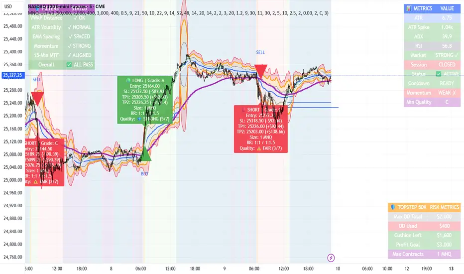
MNQ TopStep 50K | Ultra Quality v3.0MNQ TopStep 50K | Ultra Quality v3.0 - Publish Summary📊 OverviewA professional-grade trading indicator designed specifically for MNQ futures traders using TopStep funded accounts. Combines 7 technical confirmations with 5 advanced safety filters to deliver high-quality trade signals while managing drawdown risk.🎯 Key FeaturesCore Signal System
7-Point Confirmation: VWAP, EMA crossovers, 15-min HTF trend, MACD, RSI, ADX, and Volume
Signal Grading: Each signal is rated A+ through D based on 7 quality factors
Quality Threshold: Adjustable minimum grade requirement (A+, A, B, C, D)
Advanced Safety Filters (Customizable)
Mean Reversion Filter - Prevents chasing extended moves beyond VWAP bands
ATR Spike Filter - Avoids trading during extreme volatility events
EMA Spacing Filter - Ensures proper trend separation (optional)
Momentum Filter - Requires consecutive directional bars (optional)
Multi-Timeframe Confirmation - Aligns with 15-min trend (optional)
TopStep Risk Management
Real-time drawdown tracking
Position sizing calculator based on remaining cushion
Daily loss limit monitoring
Consecutive loss protection
Max trades per day limiter
Visual Components
VWAP with 1σ, 2σ, 3σ bands
EMA 9/21 with cloud fill
15-min EMA 50 for HTF trend
Comprehensive metrics dashboard
Risk management panel
Filter status panel
Detailed trade labels with entry, stops, and targets
⚙️ Default Settings (Balanced for Regular Signals)Technical Indicators
Fast EMA: 9 | Slow EMA: 21 | HTF EMA: 50 (15-min)
MACD: 10/22/9
RSI: 14 period | Thresholds: 52 (buy) / 48 (sell)
ADX: 14 period | Minimum: 20
ATR: 14 period | Stop: 2x | TP1: 2x | TP2: 3x
Volume: 1.2x average required
Session Settings
Default: 9:30 AM - 11:30 AM ET (adjustable)
Avoids first 15 minutes after market open
Customizable trading hours
Safety Filters (Default Configuration)
✅ Mean Reversion: Enabled (2.5σ max from VWAP)
✅ ATR Spike: Enabled (2.0x threshold)
❌ EMA Spacing: Disabled (can enable for quality)
❌ Momentum: Disabled (can enable for quality)
❌ MTF Confirmation: Disabled (can enable for quality)
Risk Controls
Minimum Signal Quality: C (adjustable to A+ for fewer/better signals)
Min Bars Between Signals: 10
Max Trades Per Day: 5
Stop After Consecutive Losses: 2
📈 Expected PerformanceWith Default Settings:
Signals per week: 10-15 trades
Estimated win rate: 55-60%
Risk-Reward: 1:2 (TP1) and 1:3 (TP2)
With Aggressive Settings (Min Quality = D, All Filters Off):
Signals per week: 20-25 trades
Estimated win rate: 50-55%
With Conservative Settings (Min Quality = A, All Filters On):
Signals per week: 3-5 trades
Estimated win rate: 65-70%
🚀 How to UseBasic Setup:
Add indicator to MNQ 5-minute chart
Adjust TopStep account settings in inputs
Set your risk per trade percentage (default: 0.5%)
Configure trading session hours
Set minimum signal quality (Start with C for balanced results)
Signal Interpretation:
Green Triangle (BUY): Long signal - all confirmations aligned
Red Triangle (SELL): Short signal - all confirmations aligned
Label Details: Shows entry, stop loss, take profit levels, position size, and signal grade
Signal Grade: A+ = Elite (6-7 points) | A = Strong (5) | B = Good (4) | C = Fair (3)
Dashboard Monitoring:
Top Right: Technical metrics and market conditions
Top Left: Filter status (which filters are passing/blocking)
Bottom Right: TopStep risk metrics and position sizing
⚡ Customization TipsFor More Signals:
Lower "Minimum Signal Quality" to D
Decrease ADX threshold to 18-20
Lower RSI thresholds to 50/50
Reduce Volume multiplier to 1.1x
Disable additional filters
For Higher Quality (Fewer Signals):
Raise "Minimum Signal Quality" to A or A+
Increase ADX threshold to 25-30
Enable all 5 advanced filters
Tighten VWAP distance to 2.0σ
Increase momentum requirement to 3-4 bars
For TopStep Compliance:
Adjust "Max Total Drawdown" and "Daily Loss Limit" to match your account
Update "Already Used Drawdown" daily
Monitor the Risk Panel for cushion remaining
Use recommended contract sizing
🛡️ Risk DisclaimerIMPORTANT: This indicator is for educational and informational purposes only.
Past performance does not guarantee future results
All trading involves substantial risk of loss
Use proper risk management and position sizing
Test thoroughly in paper trading before live use
The indicator does not guarantee profitable trades
Adjust settings based on your risk tolerance and trading style
Always comply with your broker's and TopStep's rules

MNQ Morning Indicator | Clean SignalsMNQ Morning Trading Indicator Summary
What It Does
This is a TradingView indicator designed for day trading MNQ (Micro Nasdaq-100 futures) during morning sessions. It generates BUY and SELL signals only when multiple technical conditions align, helping traders identify high-probability trade setups.
Core Strategy
BUY Signal Requirements (All must be true):
✅ Price above VWAP (volume-weighted average price)
✅ Fast EMA (9) above Slow EMA (21) - uptrend confirmation
✅ Price above 15-minute 50 EMA - higher timeframe confirmation
✅ MACD histogram positive - momentum confirmation
✅ RSI above 55 - strength confirmation
✅ ADX above 25 - trending market (not choppy)
✅ Volume 1.5x above average - strong participation
SELL Signal (opposite conditions)
Key Features
🎯 Risk Management
Stop Loss: 2× ATR (Average True Range)
Take Profit 1: 2× ATR (1:2 risk-reward)
Take Profit 2: 3× ATR (1:3 risk-reward)
Dollar values: Calculates P&L based on MNQ's $2/point value
⏰ Session Filter
Default: 9:30 AM - 11:30 AM ET (customizable)
Safety feature: Avoids first 15 minutes (high volatility period)
Won't generate signals outside trading hours
🛡️ Signal Quality
Rates each signal: 🔥 STRONG, ⚡ MEDIUM, or ⚠️ WEAK
Requires minimum 15 bars between signals (prevents overtrading)
📊 Visual Dashboard
Shows real-time metrics:
ATR values
ADX (trend strength)
RSI (momentum)
Market condition (TREND/CHOP)
Session status
Volume status
Signal cooldown timer
Visual Elements
📈 VWAP with standard deviation bands (1σ, 2σ, 3σ)
📉 Multiple EMAs with trend-based coloring
🟢/🔴 Buy/Sell arrows on chart
📋 Detailed trade labels showing entry, SL, TPs, and risk-reward ratios
🎨 Background highlighting for market conditions
Safety Features
Cooldown period between signals
Session restrictions (no trading outside set hours)
First 15-minute avoidance (post-open volatility)
Multi-confirmation requirement (all 7 conditions must align)
Trend filter (ADX minimum to avoid choppy markets)
Best For
Day traders focused on morning sessions
MNQ futures traders
Traders who prefer systematic, rule-based entries
Those wanting pre-calculated risk management levels
Customization
All parameters are adjustable:
EMA periods
MACD settings
RSI thresholds
ADX minimum
ATR multipliers
Session times
Visual preferences
This indicator is designed to be conservative — it waits for strong confirmation before signaling, which means fewer but potentially higher-quality trades.