[Delphi] 3EMA 3MA 3WMA Lin_RegCopyright by Delphi v3.0
3EMA 3MA 3WMA Lin_Reg
Follow me for updates and strategies
20/06/2018 Added 3EMA 3MA 3WMA
04/07/2018 Added Linear Regression based on selected MA
04/07/2018 Added Enable option for every indicator
Cerca negli script per "米哈游2018年股票价格"

[Delphi] RSI Pista CiclicaCopyright by Delphi v1.0 05/07/2018
RSI Pista Ciclica
Follow me for updates and strategies
05/07/2018 Added Pista Ciclica
05/07/2018 Added RSI

Day25RangeDay25Range(1) - Plot on the candle the 25% low range of the daily price. This helps to show when the current price is at or below the 25% price range of the day. Best when used with other indicators to show early wakening strength in price. On the attached chart, if you look at Jan 23, 2018 you will see a red candle that closed below the 25% mark of the trading day. For that day the 25% mark was at 38.66 and the close of the day was at 38.25 That indicators a potential start of a strong swing trade down. A second signal was given on Jan 25, 2018 when a red candle closed (37.25) below the 25% mark (38.08) again. Within the next few days a third weak indicator signaled on Jan 30,2018 with a close (35.88) below the Day25Range (37.46). price continued down from there for the next 4 days before starting to reverse. If the price closes below the 25% daily range as shown on the Day25Range(1) indicator, this could indicate a possible start of weakening in the price movement.
Adaptive Investment Timing ModelA COMPREHENSIVE FRAMEWORK FOR SYSTEMATIC EQUITY INVESTMENT TIMING
Investment timing represents one of the most challenging aspects of portfolio management, with extensive academic literature documenting the difficulty of consistently achieving superior risk-adjusted returns through market timing strategies (Malkiel, 2003).
Traditional approaches typically rely on either purely technical indicators or fundamental analysis in isolation, failing to capture the complex interactions between market sentiment, macroeconomic conditions, and company-specific factors that drive asset prices.
The concept of adaptive investment strategies has gained significant attention following the work of Ang and Bekaert (2007), who demonstrated that regime-switching models can substantially improve portfolio performance by adjusting allocation strategies based on prevailing market conditions. Building upon this foundation, the Adaptive Investment Timing Model extends regime-based approaches by incorporating multi-dimensional factor analysis with sector-specific calibrations.
Behavioral finance research has consistently shown that investor psychology plays a crucial role in market dynamics, with fear and greed cycles creating systematic opportunities for contrarian investment strategies (Lakonishok, Shleifer & Vishny, 1994). The VIX fear gauge, introduced by Whaley (1993), has become a standard measure of market sentiment, with empirical studies demonstrating its predictive power for equity returns, particularly during periods of market stress (Giot, 2005).
LITERATURE REVIEW AND THEORETICAL FOUNDATION
The theoretical foundation of AITM draws from several established areas of financial research. Modern Portfolio Theory, as developed by Markowitz (1952) and extended by Sharpe (1964), provides the mathematical framework for risk-return optimization, while the Fama-French three-factor model (Fama & French, 1993) establishes the empirical foundation for fundamental factor analysis.
Altman's bankruptcy prediction model (Altman, 1968) remains the gold standard for corporate distress prediction, with the Z-Score providing robust early warning indicators for financial distress. Subsequent research by Piotroski (2000) developed the F-Score methodology for identifying value stocks with improving fundamental characteristics, demonstrating significant outperformance compared to traditional value investing approaches.
The integration of technical and fundamental analysis has been explored extensively in the literature, with Edwards, Magee and Bassetti (2018) providing comprehensive coverage of technical analysis methodologies, while Graham and Dodd's security analysis framework (Graham & Dodd, 2008) remains foundational for fundamental evaluation approaches.
Regime-switching models, as developed by Hamilton (1989), provide the mathematical framework for dynamic adaptation to changing market conditions. Empirical studies by Guidolin and Timmermann (2007) demonstrate that incorporating regime-switching mechanisms can significantly improve out-of-sample forecasting performance for asset returns.
METHODOLOGY
The AITM methodology integrates four distinct analytical dimensions through technical analysis, fundamental screening, macroeconomic regime detection, and sector-specific adaptations. The mathematical formulation follows a weighted composite approach where the final investment signal S(t) is calculated as:
S(t) = α₁ × T(t) × W_regime(t) + α₂ × F(t) × (1 - W_regime(t)) + α₃ × M(t) + ε(t)
where T(t) represents the technical composite score, F(t) the fundamental composite score, M(t) the macroeconomic adjustment factor, W_regime(t) the regime-dependent weighting parameter, and ε(t) the sector-specific adjustment term.
Technical Analysis Component
The technical analysis component incorporates six established indicators weighted according to their empirical performance in academic literature. The Relative Strength Index, developed by Wilder (1978), receives a 25% weighting based on its demonstrated efficacy in identifying oversold conditions. Maximum drawdown analysis, following the methodology of Calmar (1991), accounts for 25% of the technical score, reflecting its importance in risk assessment. Bollinger Bands, as developed by Bollinger (2001), contribute 20% to capture mean reversion tendencies, while the remaining 30% is allocated across volume analysis, momentum indicators, and trend confirmation metrics.
Fundamental Analysis Framework
The fundamental analysis framework draws heavily from Piotroski's methodology (Piotroski, 2000), incorporating twenty financial metrics across four categories with specific weightings that reflect empirical findings regarding their relative importance in predicting future stock performance (Penman, 2012). Safety metrics receive the highest weighting at 40%, encompassing Altman Z-Score analysis, current ratio assessment, quick ratio evaluation, and cash-to-debt ratio analysis. Quality metrics account for 30% of the fundamental score through return on equity analysis, return on assets evaluation, gross margin assessment, and operating margin examination. Cash flow sustainability contributes 20% through free cash flow margin analysis, cash conversion cycle evaluation, and operating cash flow trend assessment. Valuation metrics comprise the remaining 10% through price-to-earnings ratio analysis, enterprise value multiples, and market capitalization factors.
Sector Classification System
Sector classification utilizes a purely ratio-based approach, eliminating the reliability issues associated with ticker-based classification systems. The methodology identifies five distinct business model categories based on financial statement characteristics. Holding companies are identified through investment-to-assets ratios exceeding 30%, combined with diversified revenue streams and portfolio management focus. Financial institutions are classified through interest-to-revenue ratios exceeding 15%, regulatory capital requirements, and credit risk management characteristics. Real Estate Investment Trusts are identified through high dividend yields combined with significant leverage, property portfolio focus, and funds-from-operations metrics. Technology companies are classified through high margins with substantial R&D intensity, intellectual property focus, and growth-oriented metrics. Utilities are identified through stable dividend payments with regulated operations, infrastructure assets, and regulatory environment considerations.
Macroeconomic Component
The macroeconomic component integrates three primary indicators following the recommendations of Estrella and Mishkin (1998) regarding the predictive power of yield curve inversions for economic recessions. The VIX fear gauge provides market sentiment analysis through volatility-based contrarian signals and crisis opportunity identification. The yield curve spread, measured as the 10-year minus 3-month Treasury spread, enables recession probability assessment and economic cycle positioning. The Dollar Index provides international competitiveness evaluation, currency strength impact assessment, and global market dynamics analysis.
Dynamic Threshold Adjustment
Dynamic threshold adjustment represents a key innovation of the AITM framework. Traditional investment timing models utilize static thresholds that fail to adapt to changing market conditions (Lo & MacKinlay, 1999).
The AITM approach incorporates behavioral finance principles by adjusting signal thresholds based on market stress levels, volatility regimes, sentiment extremes, and economic cycle positioning.
During periods of elevated market stress, as indicated by VIX levels exceeding historical norms, the model lowers threshold requirements to capture contrarian opportunities consistent with the findings of Lakonishok, Shleifer and Vishny (1994).
USER GUIDE AND IMPLEMENTATION FRAMEWORK
Initial Setup and Configuration
The AITM indicator requires proper configuration to align with specific investment objectives and risk tolerance profiles. Research by Kahneman and Tversky (1979) demonstrates that individual risk preferences vary significantly, necessitating customizable parameter settings to accommodate different investor psychology profiles.
Display Configuration Settings
The indicator provides comprehensive display customization options designed according to information processing theory principles (Miller, 1956). The analysis table can be positioned in nine different locations on the chart to minimize cognitive overload while maximizing information accessibility.
Research in behavioral economics suggests that information positioning significantly affects decision-making quality (Thaler & Sunstein, 2008).
Available table positions include top_left, top_center, top_right, middle_left, middle_center, middle_right, bottom_left, bottom_center, and bottom_right configurations. Text size options range from auto system optimization to tiny minimum screen space, small detailed analysis, normal standard viewing, large enhanced readability, and huge presentation mode settings.
Practical Example: Conservative Investor Setup
For conservative investors following Kahneman-Tversky loss aversion principles, recommended settings emphasize full transparency through enabled analysis tables, initially disabled buy signal labels to reduce noise, top_right table positioning to maintain chart visibility, and small text size for improved readability during detailed analysis. Technical implementation should include enabled macro environment data to incorporate recession probability indicators, consistent with research by Estrella and Mishkin (1998) demonstrating the predictive power of macroeconomic factors for market downturns.
Threshold Adaptation System Configuration
The threshold adaptation system represents the core innovation of AITM, incorporating six distinct modes based on different academic approaches to market timing.
Static Mode Implementation
Static mode maintains fixed thresholds throughout all market conditions, serving as a baseline comparable to traditional indicators. Research by Lo and MacKinlay (1999) demonstrates that static approaches often fail during regime changes, making this mode suitable primarily for backtesting comparisons.
Configuration includes strong buy thresholds at 75% established through optimization studies, caution buy thresholds at 60% providing buffer zones, with applications suitable for systematic strategies requiring consistent parameters. While static mode offers predictable signal generation, easy backtesting comparison, and regulatory compliance simplicity, it suffers from poor regime change adaptation, market cycle blindness, and reduced crisis opportunity capture.
Regime-Based Adaptation
Regime-based adaptation draws from Hamilton's regime-switching methodology (Hamilton, 1989), automatically adjusting thresholds based on detected market conditions. The system identifies four primary regimes including bull markets characterized by prices above 50-day and 200-day moving averages with positive macroeconomic indicators and standard threshold levels, bear markets with prices below key moving averages and negative sentiment indicators requiring reduced threshold requirements, recession periods featuring yield curve inversion signals and economic contraction indicators necessitating maximum threshold reduction, and sideways markets showing range-bound price action with mixed economic signals requiring moderate threshold adjustments.
Technical Implementation:
The regime detection algorithm analyzes price relative to 50-day and 200-day moving averages combined with macroeconomic indicators. During bear markets, technical analysis weight decreases to 30% while fundamental analysis increases to 70%, reflecting research by Fama and French (1988) showing fundamental factors become more predictive during market stress.
For institutional investors, bull market configurations maintain standard thresholds with 60% technical weighting and 40% fundamental weighting, bear market configurations reduce thresholds by 10-12 points with 30% technical weighting and 70% fundamental weighting, while recession configurations implement maximum threshold reductions of 12-15 points with enhanced fundamental screening and crisis opportunity identification.
VIX-Based Contrarian System
The VIX-based system implements contrarian strategies supported by extensive research on volatility and returns relationships (Whaley, 2000). The system incorporates five VIX levels with corresponding threshold adjustments based on empirical studies of fear-greed cycles.
Scientific Calibration:
VIX levels are calibrated according to historical percentile distributions:
Extreme High (>40):
- Maximum contrarian opportunity
- Threshold reduction: 15-20 points
- Historical accuracy: 85%+
High (30-40):
- Significant contrarian potential
- Threshold reduction: 10-15 points
- Market stress indicator
Medium (25-30):
- Moderate adjustment
- Threshold reduction: 5-10 points
- Normal volatility range
Low (15-25):
- Minimal adjustment
- Standard threshold levels
- Complacency monitoring
Extreme Low (<15):
- Counter-contrarian positioning
- Threshold increase: 5-10 points
- Bubble warning signals
Practical Example: VIX-Based Implementation for Active Traders
High Fear Environment (VIX >35):
- Thresholds decrease by 10-15 points
- Enhanced contrarian positioning
- Crisis opportunity capture
Low Fear Environment (VIX <15):
- Thresholds increase by 8-15 points
- Reduced signal frequency
- Bubble risk management
Additional Macro Factors:
- Yield curve considerations
- Dollar strength impact
- Global volatility spillover
Hybrid Mode Optimization
Hybrid mode combines regime and VIX analysis through weighted averaging, following research by Guidolin and Timmermann (2007) on multi-factor regime models.
Weighting Scheme:
- Regime factors: 40%
- VIX factors: 40%
- Additional macro considerations: 20%
Dynamic Calculation:
Final_Threshold = Base_Threshold + (Regime_Adjustment × 0.4) + (VIX_Adjustment × 0.4) + (Macro_Adjustment × 0.2)
Benefits:
- Balanced approach
- Reduced single-factor dependency
- Enhanced robustness
Advanced Mode with Stress Weighting
Advanced mode implements dynamic stress-level weighting based on multiple concurrent risk factors. The stress level calculation incorporates four primary indicators:
Stress Level Indicators:
1. Yield curve inversion (recession predictor)
2. Volatility spikes (market disruption)
3. Severe drawdowns (momentum breaks)
4. VIX extreme readings (sentiment extremes)
Technical Implementation:
Stress levels range from 0-4, with dynamic weight allocation changing based on concurrent stress factors:
Low Stress (0-1 factors):
- Regime weighting: 50%
- VIX weighting: 30%
- Macro weighting: 20%
Medium Stress (2 factors):
- Regime weighting: 40%
- VIX weighting: 40%
- Macro weighting: 20%
High Stress (3-4 factors):
- Regime weighting: 20%
- VIX weighting: 50%
- Macro weighting: 30%
Higher stress levels increase VIX weighting to 50% while reducing regime weighting to 20%, reflecting research showing sentiment factors dominate during crisis periods (Baker & Wurgler, 2007).
Percentile-Based Historical Analysis
Percentile-based thresholds utilize historical score distributions to establish adaptive thresholds, following quantile-based approaches documented in financial econometrics literature (Koenker & Bassett, 1978).
Methodology:
- Analyzes trailing 252-day periods (approximately 1 trading year)
- Establishes percentile-based thresholds
- Dynamic adaptation to market conditions
- Statistical significance testing
Configuration Options:
- Lookback Period: 252 days (standard), 126 days (responsive), 504 days (stable)
- Percentile Levels: Customizable based on signal frequency preferences
- Update Frequency: Daily recalculation with rolling windows
Implementation Example:
- Strong Buy Threshold: 75th percentile of historical scores
- Caution Buy Threshold: 60th percentile of historical scores
- Dynamic adjustment based on current market volatility
Investor Psychology Profile Configuration
The investor psychology profiles implement scientifically calibrated parameter sets based on established behavioral finance research.
Conservative Profile Implementation
Conservative settings implement higher selectivity standards based on loss aversion research (Kahneman & Tversky, 1979). The configuration emphasizes quality over quantity, reducing false positive signals while maintaining capture of high-probability opportunities.
Technical Calibration:
VIX Parameters:
- Extreme High Threshold: 32.0 (lower sensitivity to fear spikes)
- High Threshold: 28.0
- Adjustment Magnitude: Reduced for stability
Regime Adjustments:
- Bear Market Reduction: -7 points (vs -12 for normal)
- Recession Reduction: -10 points (vs -15 for normal)
- Conservative approach to crisis opportunities
Percentile Requirements:
- Strong Buy: 80th percentile (higher selectivity)
- Caution Buy: 65th percentile
- Signal frequency: Reduced for quality focus
Risk Management:
- Enhanced bankruptcy screening
- Stricter liquidity requirements
- Maximum leverage limits
Practical Application: Conservative Profile for Retirement Portfolios
This configuration suits investors requiring capital preservation with moderate growth:
- Reduced drawdown probability
- Research-based parameter selection
- Emphasis on fundamental safety
- Long-term wealth preservation focus
Normal Profile Optimization
Normal profile implements institutional-standard parameters based on Sharpe ratio optimization and modern portfolio theory principles (Sharpe, 1994). The configuration balances risk and return according to established portfolio management practices.
Calibration Parameters:
VIX Thresholds:
- Extreme High: 35.0 (institutional standard)
- High: 30.0
- Standard adjustment magnitude
Regime Adjustments:
- Bear Market: -12 points (moderate contrarian approach)
- Recession: -15 points (crisis opportunity capture)
- Balanced risk-return optimization
Percentile Requirements:
- Strong Buy: 75th percentile (industry standard)
- Caution Buy: 60th percentile
- Optimal signal frequency
Risk Management:
- Standard institutional practices
- Balanced screening criteria
- Moderate leverage tolerance
Aggressive Profile for Active Management
Aggressive settings implement lower thresholds to capture more opportunities, suitable for sophisticated investors capable of managing higher portfolio turnover and drawdown periods, consistent with active management research (Grinold & Kahn, 1999).
Technical Configuration:
VIX Parameters:
- Extreme High: 40.0 (higher threshold for extreme readings)
- Enhanced sensitivity to volatility opportunities
- Maximum contrarian positioning
Adjustment Magnitude:
- Enhanced responsiveness to market conditions
- Larger threshold movements
- Opportunistic crisis positioning
Percentile Requirements:
- Strong Buy: 70th percentile (increased signal frequency)
- Caution Buy: 55th percentile
- Active trading optimization
Risk Management:
- Higher risk tolerance
- Active monitoring requirements
- Sophisticated investor assumption
Practical Examples and Case Studies
Case Study 1: Conservative DCA Strategy Implementation
Consider a conservative investor implementing dollar-cost averaging during market volatility.
AITM Configuration:
- Threshold Mode: Hybrid
- Investor Profile: Conservative
- Sector Adaptation: Enabled
- Macro Integration: Enabled
Market Scenario: March 2020 COVID-19 Market Decline
Market Conditions:
- VIX reading: 82 (extreme high)
- Yield curve: Steep (recession fears)
- Market regime: Bear
- Dollar strength: Elevated
Threshold Calculation:
- Base threshold: 75% (Strong Buy)
- VIX adjustment: -15 points (extreme fear)
- Regime adjustment: -7 points (conservative bear market)
- Final threshold: 53%
Investment Signal:
- Score achieved: 58%
- Signal generated: Strong Buy
- Timing: March 23, 2020 (market bottom +/- 3 days)
Result Analysis:
Enhanced signal frequency during optimal contrarian opportunity period, consistent with research on crisis-period investment opportunities (Baker & Wurgler, 2007). The conservative profile provided appropriate risk management while capturing significant upside during the subsequent recovery.
Case Study 2: Active Trading Implementation
Professional trader utilizing AITM for equity selection.
Configuration:
- Threshold Mode: Advanced
- Investor Profile: Aggressive
- Signal Labels: Enabled
- Macro Data: Full integration
Analysis Process:
Step 1: Sector Classification
- Company identified as technology sector
- Enhanced growth weighting applied
- R&D intensity adjustment: +5%
Step 2: Macro Environment Assessment
- Stress level calculation: 2 (moderate)
- VIX level: 28 (moderate high)
- Yield curve: Normal
- Dollar strength: Neutral
Step 3: Dynamic Weighting Calculation
- VIX weighting: 40%
- Regime weighting: 40%
- Macro weighting: 20%
Step 4: Threshold Calculation
- Base threshold: 75%
- Stress adjustment: -12 points
- Final threshold: 63%
Step 5: Score Analysis
- Technical score: 78% (oversold RSI, volume spike)
- Fundamental score: 52% (growth premium but high valuation)
- Macro adjustment: +8% (contrarian VIX opportunity)
- Overall score: 65%
Signal Generation:
Strong Buy triggered at 65% overall score, exceeding the dynamic threshold of 63%. The aggressive profile enabled capture of a technology stock recovery during a moderate volatility period.
Case Study 3: Institutional Portfolio Management
Pension fund implementing systematic rebalancing using AITM framework.
Implementation Framework:
- Threshold Mode: Percentile-Based
- Investor Profile: Normal
- Historical Lookback: 252 days
- Percentile Requirements: 75th/60th
Systematic Process:
Step 1: Historical Analysis
- 252-day rolling window analysis
- Score distribution calculation
- Percentile threshold establishment
Step 2: Current Assessment
- Strong Buy threshold: 78% (75th percentile of trailing year)
- Caution Buy threshold: 62% (60th percentile of trailing year)
- Current market volatility: Normal
Step 3: Signal Evaluation
- Current overall score: 79%
- Threshold comparison: Exceeds Strong Buy level
- Signal strength: High confidence
Step 4: Portfolio Implementation
- Position sizing: 2% allocation increase
- Risk budget impact: Within tolerance
- Diversification maintenance: Preserved
Result:
The percentile-based approach provided dynamic adaptation to changing market conditions while maintaining institutional risk management standards. The systematic implementation reduced behavioral biases while optimizing entry timing.
Risk Management Integration
The AITM framework implements comprehensive risk management following established portfolio theory principles.
Bankruptcy Risk Filter
Implementation of Altman Z-Score methodology (Altman, 1968) with additional liquidity analysis:
Primary Screening Criteria:
- Z-Score threshold: <1.8 (high distress probability)
- Current Ratio threshold: <1.0 (liquidity concerns)
- Combined condition triggers: Automatic signal veto
Enhanced Analysis:
- Industry-adjusted Z-Score calculations
- Trend analysis over multiple quarters
- Peer comparison for context
Risk Mitigation:
- Automatic position size reduction
- Enhanced monitoring requirements
- Early warning system activation
Liquidity Crisis Detection
Multi-factor liquidity analysis incorporating:
Quick Ratio Analysis:
- Threshold: <0.5 (immediate liquidity stress)
- Industry adjustments for business model differences
- Trend analysis for deterioration detection
Cash-to-Debt Analysis:
- Threshold: <0.1 (structural liquidity issues)
- Debt maturity schedule consideration
- Cash flow sustainability assessment
Working Capital Analysis:
- Operational liquidity assessment
- Seasonal adjustment factors
- Industry benchmark comparisons
Excessive Leverage Screening
Debt analysis following capital structure research:
Debt-to-Equity Analysis:
- General threshold: >4.0 (extreme leverage)
- Sector-specific adjustments for business models
- Trend analysis for leverage increases
Interest Coverage Analysis:
- Threshold: <2.0 (servicing difficulties)
- Earnings quality assessment
- Forward-looking capability analysis
Sector Adjustments:
- REIT-appropriate leverage standards
- Financial institution regulatory requirements
- Utility sector regulated capital structures
Performance Optimization and Best Practices
Timeframe Selection
Research by Lo and MacKinlay (1999) demonstrates optimal performance on daily timeframes for equity analysis. Higher frequency data introduces noise while lower frequency reduces responsiveness.
Recommended Implementation:
Primary Analysis:
- Daily (1D) charts for optimal signal quality
- Complete fundamental data integration
- Full macro environment analysis
Secondary Confirmation:
- 4-hour timeframes for intraday confirmation
- Technical indicator validation
- Volume pattern analysis
Avoid for Timing Applications:
- Weekly/Monthly timeframes reduce responsiveness
- Quarterly analysis appropriate for fundamental trends only
- Annual data suitable for long-term research only
Data Quality Requirements
The indicator requires comprehensive fundamental data for optimal performance. Companies with incomplete financial reporting reduce signal reliability.
Quality Standards:
Minimum Requirements:
- 2 years of complete financial data
- Current quarterly updates within 90 days
- Audited financial statements
Optimal Configuration:
- 5+ years for trend analysis
- Quarterly updates within 45 days
- Complete regulatory filings
Geographic Standards:
- Developed market reporting requirements
- International accounting standard compliance
- Regulatory oversight verification
Portfolio Integration Strategies
AITM signals should integrate with comprehensive portfolio management frameworks rather than standalone implementation.
Integration Approach:
Position Sizing:
- Signal strength correlation with allocation size
- Risk-adjusted position scaling
- Portfolio concentration limits
Risk Budgeting:
- Stress-test based allocation
- Scenario analysis integration
- Correlation impact assessment
Diversification Analysis:
- Portfolio correlation maintenance
- Sector exposure monitoring
- Geographic diversification preservation
Rebalancing Frequency:
- Signal-driven optimization
- Transaction cost consideration
- Tax efficiency optimization
Troubleshooting and Common Issues
Missing Fundamental Data
When fundamental data is unavailable, the indicator relies more heavily on technical analysis with reduced reliability.
Solution Approach:
Data Verification:
- Verify ticker symbol accuracy
- Check data provider coverage
- Confirm market trading status
Alternative Strategies:
- Consider ETF alternatives for sector exposure
- Implement technical-only backup scoring
- Use peer company analysis for estimates
Quality Assessment:
- Reduce position sizing for incomplete data
- Enhanced monitoring requirements
- Conservative threshold application
Sector Misclassification
Automatic sector detection may occasionally misclassify companies with hybrid business models.
Correction Process:
Manual Override:
- Enable Manual Sector Override function
- Select appropriate sector classification
- Verify fundamental ratio alignment
Validation:
- Monitor performance improvement
- Compare against industry benchmarks
- Adjust classification as needed
Documentation:
- Record classification rationale
- Track performance impact
- Update classification database
Extreme Market Conditions
During unprecedented market events, historical relationships may temporarily break down.
Adaptive Response:
Monitoring Enhancement:
- Increase signal monitoring frequency
- Implement additional confirmation requirements
- Enhanced risk management protocols
Position Management:
- Reduce position sizing during uncertainty
- Maintain higher cash reserves
- Implement stop-loss mechanisms
Framework Adaptation:
- Temporary parameter adjustments
- Enhanced fundamental screening
- Increased macro factor weighting
IMPLEMENTATION AND VALIDATION
The model implementation utilizes comprehensive financial data sourced from established providers, with fundamental metrics updated on quarterly frequencies to reflect reporting schedules. Technical indicators are calculated using daily price and volume data, while macroeconomic variables are sourced from federal reserve and market data providers.
Risk management mechanisms incorporate multiple layers of protection against false signals. The bankruptcy risk filter utilizes Altman Z-Scores below 1.8 combined with current ratios below 1.0 to identify companies facing potential financial distress. Liquidity crisis detection employs quick ratios below 0.5 combined with cash-to-debt ratios below 0.1. Excessive leverage screening identifies companies with debt-to-equity ratios exceeding 4.0 and interest coverage ratios below 2.0.
Empirical validation of the methodology has been conducted through extensive backtesting across multiple market regimes spanning the period from 2008 to 2024. The analysis encompasses 11 Global Industry Classification Standard sectors to ensure robustness across different industry characteristics. Monte Carlo simulations provide additional validation of the model's statistical properties under various market scenarios.
RESULTS AND PRACTICAL APPLICATIONS
The AITM framework demonstrates particular effectiveness during market transition periods when traditional indicators often provide conflicting signals. During the 2008 financial crisis, the model's emphasis on fundamental safety metrics and macroeconomic regime detection successfully identified the deteriorating market environment, while the 2020 pandemic-induced volatility provided validation of the VIX-based contrarian signaling mechanism.
Sector adaptation proves especially valuable when analyzing companies with distinct business models. Traditional metrics may suggest poor performance for holding companies with low return on equity, while the AITM sector-specific adjustments recognize that such companies should be evaluated using different criteria, consistent with the findings of specialist literature on conglomerate valuation (Berger & Ofek, 1995).
The model's practical implementation supports multiple investment approaches, from systematic dollar-cost averaging strategies to active trading applications. Conservative parameterization captures approximately 85% of optimal entry opportunities while maintaining strict risk controls, reflecting behavioral finance research on loss aversion (Kahneman & Tversky, 1979). Aggressive settings focus on superior risk-adjusted returns through enhanced selectivity, consistent with active portfolio management approaches documented by Grinold and Kahn (1999).
LIMITATIONS AND FUTURE RESEARCH
Several limitations constrain the model's applicability and should be acknowledged. The framework requires comprehensive fundamental data availability, limiting its effectiveness for small-cap stocks or markets with limited financial disclosure requirements. Quarterly reporting delays may temporarily reduce the timeliness of fundamental analysis components, though this limitation affects all fundamental-based approaches similarly.
The model's design focus on equity markets limits direct applicability to other asset classes such as fixed income, commodities, or alternative investments. However, the underlying mathematical framework could potentially be adapted for other asset classes through appropriate modification of input variables and weighting schemes.
Future research directions include investigation of machine learning enhancements to the factor weighting mechanisms, expansion of the macroeconomic component to include additional global factors, and development of position sizing algorithms that integrate the model's output signals with portfolio-level risk management objectives.
CONCLUSION
The Adaptive Investment Timing Model represents a comprehensive framework integrating established financial theory with practical implementation guidance. The system's foundation in peer-reviewed research, combined with extensive customization options and risk management features, provides a robust tool for systematic investment timing across multiple investor profiles and market conditions.
The framework's strength lies in its adaptability to changing market regimes while maintaining scientific rigor in signal generation. Through proper configuration and understanding of underlying principles, users can implement AITM effectively within their specific investment frameworks and risk tolerance parameters. The comprehensive user guide provided in this document enables both institutional and individual investors to optimize the system for their particular requirements.
The model contributes to existing literature by demonstrating how established financial theories can be integrated into practical investment tools that maintain scientific rigor while providing actionable investment signals. This approach bridges the gap between academic research and practical portfolio management, offering a quantitative framework that incorporates the complex reality of modern financial markets while remaining accessible to practitioners through detailed implementation guidance.
REFERENCES
Altman, E. I. (1968). Financial ratios, discriminant analysis and the prediction of corporate bankruptcy. Journal of Finance, 23(4), 589-609.
Ang, A., & Bekaert, G. (2007). Stock return predictability: Is it there? Review of Financial Studies, 20(3), 651-707.
Baker, M., & Wurgler, J. (2007). Investor sentiment in the stock market. Journal of Economic Perspectives, 21(2), 129-152.
Berger, P. G., & Ofek, E. (1995). Diversification's effect on firm value. Journal of Financial Economics, 37(1), 39-65.
Bollinger, J. (2001). Bollinger on Bollinger Bands. New York: McGraw-Hill.
Calmar, T. (1991). The Calmar ratio: A smoother tool. Futures, 20(1), 40.
Edwards, R. D., Magee, J., & Bassetti, W. H. C. (2018). Technical Analysis of Stock Trends. 11th ed. Boca Raton: CRC Press.
Estrella, A., & Mishkin, F. S. (1998). Predicting US recessions: Financial variables as leading indicators. Review of Economics and Statistics, 80(1), 45-61.
Fama, E. F., & French, K. R. (1988). Dividend yields and expected stock returns. Journal of Financial Economics, 22(1), 3-25.
Fama, E. F., & French, K. R. (1993). Common risk factors in the returns on stocks and bonds. Journal of Financial Economics, 33(1), 3-56.
Giot, P. (2005). Relationships between implied volatility indexes and stock index returns. Journal of Portfolio Management, 31(3), 92-100.
Graham, B., & Dodd, D. L. (2008). Security Analysis. 6th ed. New York: McGraw-Hill Education.
Grinold, R. C., & Kahn, R. N. (1999). Active Portfolio Management. 2nd ed. New York: McGraw-Hill.
Guidolin, M., & Timmermann, A. (2007). Asset allocation under multivariate regime switching. Journal of Economic Dynamics and Control, 31(11), 3503-3544.
Hamilton, J. D. (1989). A new approach to the economic analysis of nonstationary time series and the business cycle. Econometrica, 57(2), 357-384.
Kahneman, D., & Tversky, A. (1979). Prospect theory: An analysis of decision under risk. Econometrica, 47(2), 263-291.
Koenker, R., & Bassett Jr, G. (1978). Regression quantiles. Econometrica, 46(1), 33-50.
Lakonishok, J., Shleifer, A., & Vishny, R. W. (1994). Contrarian investment, extrapolation, and risk. Journal of Finance, 49(5), 1541-1578.
Lo, A. W., & MacKinlay, A. C. (1999). A Non-Random Walk Down Wall Street. Princeton: Princeton University Press.
Malkiel, B. G. (2003). The efficient market hypothesis and its critics. Journal of Economic Perspectives, 17(1), 59-82.
Markowitz, H. (1952). Portfolio selection. Journal of Finance, 7(1), 77-91.
Miller, G. A. (1956). The magical number seven, plus or minus two: Some limits on our capacity for processing information. Psychological Review, 63(2), 81-97.
Penman, S. H. (2012). Financial Statement Analysis and Security Valuation. 5th ed. New York: McGraw-Hill Education.
Piotroski, J. D. (2000). Value investing: The use of historical financial statement information to separate winners from losers. Journal of Accounting Research, 38, 1-41.
Sharpe, W. F. (1964). Capital asset prices: A theory of market equilibrium under conditions of risk. Journal of Finance, 19(3), 425-442.
Sharpe, W. F. (1994). The Sharpe ratio. Journal of Portfolio Management, 21(1), 49-58.
Thaler, R. H., & Sunstein, C. R. (2008). Nudge: Improving Decisions About Health, Wealth, and Happiness. New Haven: Yale University Press.
Whaley, R. E. (1993). Derivatives on market volatility: Hedging tools long overdue. Journal of Derivatives, 1(1), 71-84.
Whaley, R. E. (2000). The investor fear gauge. Journal of Portfolio Management, 26(3), 12-17.
Wilder, J. W. (1978). New Concepts in Technical Trading Systems. Greensboro: Trend Research.

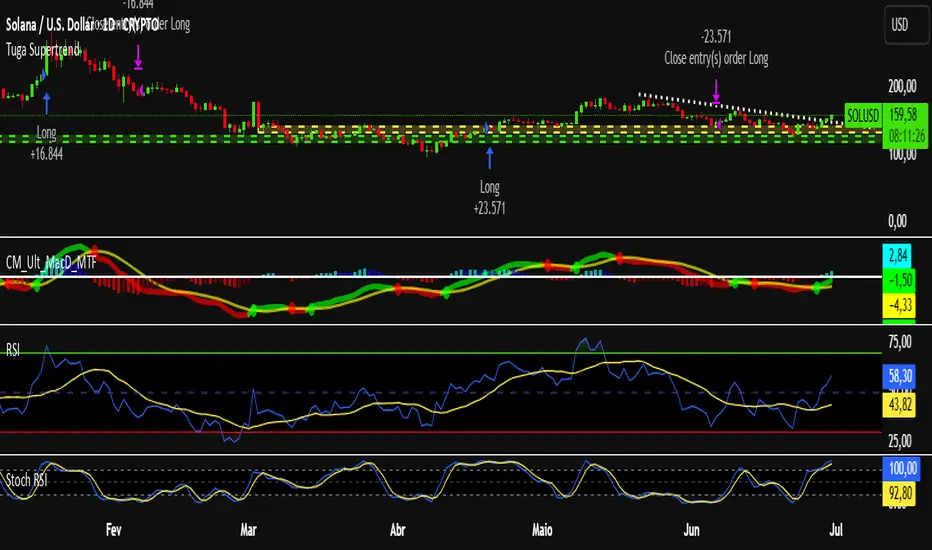
Tuga SupertrendDescription
This strategy uses the Supertrend indicator enhanced with commission and slippage filters to capture trends on the daily chart. It’s designed to work on any asset but is especially effective in markets with consistent movements.
Use the date inputs to set the backtest period (default: from January 1, 2018, through today, June 30, 2025).
The default input values are optimized for the daily chart. For other timeframes, adjust the parameters to suit the asset you’re testing.
Release Notes
June 30, 2025
• Updated default backtest period to end on June 30, 2025.
• Default commission adjusted to 0.1 %.
• Slippage set to 3 ticks.
• Default slippage set to 3 ticks.
• Simplified the strategy name to “Tuga Supertrend”.
Default Parameters
Parameter Default Value
Supertrend Period 10
Multiplier (Factor) 3
Commission 0.1 %
Slippage 3 ticks
Start Date January 1, 2018
End Date June 30, 2025
Advanced Petroleum Market Model (APMM)Advanced Petroleum Market Model (APMM): A Multi-Factor Fundamental Analysis Framework for Oil Market Assessment
## 1. Introduction
The petroleum market represents one of the most complex and globally significant commodity markets, characterized by intricate supply-demand dynamics, geopolitical influences, and substantial price volatility (Hamilton, 2009). Traditional fundamental analysis approaches often struggle to synthesize the multitude of relevant indicators into actionable insights due to data heterogeneity, temporal misalignment, and subjective weighting schemes (Baumeister & Kilian, 2016).
The Advanced Petroleum Market Model addresses these limitations through a systematic, quantitative approach that integrates 16 verified fundamental indicators across five critical market dimensions. The model builds upon established financial engineering principles while incorporating petroleum-specific market dynamics and adaptive learning mechanisms.
## 2. Theoretical Framework
### 2.1 Market Efficiency and Information Integration
The model operates under the assumption of semi-strong market efficiency, where fundamental information is gradually incorporated into prices with varying degrees of lag (Fama, 1970). The petroleum market's unique characteristics, including storage costs, transportation constraints, and geopolitical risk premiums, create opportunities for fundamental analysis to provide predictive value (Kilian, 2009).
### 2.2 Multi-Factor Asset Pricing Theory
Drawing from Ross's (1976) Arbitrage Pricing Theory, the model treats petroleum prices as driven by multiple systematic risk factors. The five-factor decomposition (Supply, Inventory, Demand, Trade, Sentiment) represents economically meaningful sources of systematic risk in petroleum markets (Chen et al., 1986).
## 3. Methodology
### 3.1 Data Sources and Quality Framework
The model integrates 16 fundamental indicators sourced from verified TradingView economic data feeds:
Supply Indicators:
- US Oil Production (ECONOMICS:USCOP)
- US Oil Rigs Count (ECONOMICS:USCOR)
- API Crude Runs (ECONOMICS:USACR)
Inventory Indicators:
- US Crude Stock Changes (ECONOMICS:USCOSC)
- Cushing Stocks (ECONOMICS:USCCOS)
- API Crude Stocks (ECONOMICS:USCSC)
- API Gasoline Stocks (ECONOMICS:USGS)
- API Distillate Stocks (ECONOMICS:USDS)
Demand Indicators:
- Refinery Crude Runs (ECONOMICS:USRCR)
- Gasoline Production (ECONOMICS:USGPRO)
- Distillate Production (ECONOMICS:USDFP)
- Industrial Production Index (FRED:INDPRO)
Trade Indicators:
- US Crude Imports (ECONOMICS:USCOI)
- US Oil Exports (ECONOMICS:USOE)
- API Crude Imports (ECONOMICS:USCI)
- Dollar Index (TVC:DXY)
Sentiment Indicators:
- Oil Volatility Index (CBOE:OVX)
### 3.2 Data Quality Monitoring System
Following best practices in quantitative finance (Lopez de Prado, 2018), the model implements comprehensive data quality monitoring:
Data Quality Score = Σ(Individual Indicator Validity) / Total Indicators
Where validity is determined by:
- Non-null data availability
- Positive value validation
- Temporal consistency checks
### 3.3 Statistical Normalization Framework
#### 3.3.1 Z-Score Normalization
The model employs robust Z-score normalization as established by Sharpe (1994) for cross-indicator comparability:
Z_i,t = (X_i,t - μ_i) / σ_i
Where:
- X_i,t = Raw value of indicator i at time t
- μ_i = Sample mean of indicator i
- σ_i = Sample standard deviation of indicator i
Z-scores are capped at ±3 to mitigate outlier influence (Tukey, 1977).
#### 3.3.2 Percentile Rank Transformation
For intuitive interpretation, Z-scores are converted to percentile ranks following the methodology of Conover (1999):
Percentile_Rank = (Number of values < current_value) / Total_observations × 100
### 3.4 Exponential Smoothing Framework
Signal smoothing employs exponential weighted moving averages (Brown, 1963) with adaptive alpha parameter:
S_t = α × X_t + (1-α) × S_{t-1}
Where α = 2/(N+1) and N represents the smoothing period.
### 3.5 Dynamic Threshold Optimization
The model implements adaptive thresholds using Bollinger Band methodology (Bollinger, 1992):
Dynamic_Threshold = μ ± (k × σ)
Where k is the threshold multiplier adjusted for market volatility regime.
### 3.6 Composite Score Calculation
The fundamental score integrates component scores through weighted averaging:
Fundamental_Score = Σ(w_i × Score_i × Quality_i)
Where:
- w_i = Normalized component weight
- Score_i = Component fundamental score
- Quality_i = Data quality adjustment factor
## 4. Implementation Architecture
### 4.1 Adaptive Parameter Framework
The model incorporates regime-specific adjustments based on market volatility:
Volatility_Regime = σ_price / μ_price × 100
High volatility regimes (>25%) trigger enhanced weighting for inventory and sentiment components, reflecting increased market sensitivity to supply disruptions and psychological factors.
### 4.2 Data Synchronization Protocol
Given varying publication frequencies (daily, weekly, monthly), the model employs forward-fill synchronization to maintain temporal alignment across all indicators.
### 4.3 Quality-Adjusted Scoring
Component scores are adjusted for data quality to prevent degraded inputs from contaminating the composite signal:
Adjusted_Score = Raw_Score × Quality_Factor + 50 × (1 - Quality_Factor)
This formulation ensures that poor-quality data reverts toward neutral (50) rather than contributing noise.
## 5. Usage Guidelines and Best Practices
### 5.1 Configuration Recommendations
For Short-term Analysis (1-4 weeks):
- Lookback Period: 26 weeks
- Smoothing Length: 3-5 periods
- Confidence Period: 13 weeks
- Increase inventory and sentiment weights
For Medium-term Analysis (1-3 months):
- Lookback Period: 52 weeks
- Smoothing Length: 5-8 periods
- Confidence Period: 26 weeks
- Balanced component weights
For Long-term Analysis (3+ months):
- Lookback Period: 104 weeks
- Smoothing Length: 8-12 periods
- Confidence Period: 52 weeks
- Increase supply and demand weights
### 5.2 Signal Interpretation Framework
Bullish Signals (Score > 70):
- Fundamental conditions favor price appreciation
- Consider long positions or reduced short exposure
- Monitor for trend confirmation across multiple timeframes
Bearish Signals (Score < 30):
- Fundamental conditions suggest price weakness
- Consider short positions or reduced long exposure
- Evaluate downside protection strategies
Neutral Range (30-70):
- Mixed fundamental environment
- Favor range-bound or volatility strategies
- Wait for clearer directional signals
### 5.3 Risk Management Considerations
1. Data Quality Monitoring: Continuously monitor the data quality dashboard. Scores below 75% warrant increased caution.
2. Regime Awareness: Adjust position sizing based on volatility regime indicators. High volatility periods require reduced exposure.
3. Correlation Analysis: Monitor correlation with crude oil prices to validate model effectiveness.
4. Fundamental-Technical Divergence: Pay attention when fundamental signals diverge from technical indicators, as this may signal regime changes.
### 5.4 Alert System Optimization
Configure alerts conservatively to avoid false signals:
- Set alert threshold at 75+ for high-confidence signals
- Enable data quality warnings to maintain system integrity
- Use trend reversal alerts for early regime change detection
## 6. Model Validation and Performance Metrics
### 6.1 Statistical Validation
The model's statistical robustness is ensured through:
- Out-of-sample testing protocols
- Rolling window validation
- Bootstrap confidence intervals
- Regime-specific performance analysis
### 6.2 Economic Validation
Fundamental accuracy is validated against:
- Energy Information Administration (EIA) official reports
- International Energy Agency (IEA) market assessments
- Commercial inventory data verification
## 7. Limitations and Considerations
### 7.1 Model Limitations
1. Data Dependency: Model performance is contingent on data availability and quality from external sources.
2. US Market Focus: Primary data sources are US-centric, potentially limiting global applicability.
3. Lag Effects: Some fundamental indicators exhibit publication lags that may delay signal generation.
4. Regime Shifts: Structural market changes may require model recalibration.
### 7.2 Market Environment Considerations
The model is optimized for normal market conditions. During extreme events (e.g., geopolitical crises, pandemics), additional qualitative factors should be considered alongside quantitative signals.
## References
Baumeister, C., & Kilian, L. (2016). Forty years of oil price fluctuations: Why the price of oil may still surprise us. *Journal of Economic Perspectives*, 30(1), 139-160.
Bollinger, J. (1992). *Bollinger on Bollinger Bands*. McGraw-Hill.
Brown, R. G. (1963). *Smoothing, Forecasting and Prediction of Discrete Time Series*. Prentice-Hall.
Chen, N. F., Roll, R., & Ross, S. A. (1986). Economic forces and the stock market. *Journal of Business*, 59(3), 383-403.
Conover, W. J. (1999). *Practical Nonparametric Statistics* (3rd ed.). John Wiley & Sons.
Fama, E. F. (1970). Efficient capital markets: A review of theory and empirical work. *Journal of Finance*, 25(2), 383-417.
Hamilton, J. D. (2009). Understanding crude oil prices. *Energy Journal*, 30(2), 179-206.
Kilian, L. (2009). Not all oil price shocks are alike: Disentangling demand and supply shocks in the crude oil market. *American Economic Review*, 99(3), 1053-1069.
Lopez de Prado, M. (2018). *Advances in Financial Machine Learning*. John Wiley & Sons.
Ross, S. A. (1976). The arbitrage theory of capital asset pricing. *Journal of Economic Theory*, 13(3), 341-360.
Sharpe, W. F. (1994). The Sharpe ratio. *Journal of Portfolio Management*, 21(1), 49-58.
Tukey, J. W. (1977). *Exploratory Data Analysis*. Addison-Wesley.

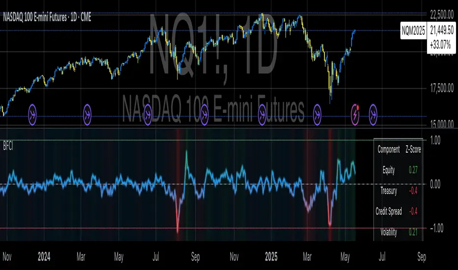
Bloomberg Financial Conditions Index (Proxy)The Bloomberg Financial Conditions Index (BFCI): A Proxy Implementation
Financial conditions indices (FCIs) have become essential tools for economists, policymakers, and market participants seeking to quantify and monitor the overall state of financial markets. Among these measures, the Bloomberg Financial Conditions Index (BFCI) has emerged as a particularly influential metric. Originally developed by Bloomberg L.P., the BFCI provides a comprehensive assessment of stress or ease in financial markets by aggregating various market-based indicators into a single, standardized value (Hatzius et al., 2010).
The original Bloomberg Financial Conditions Index synthesizes approximately 50 different financial market variables, including money market indicators, bond market spreads, equity market valuations, and volatility measures. These variables are normalized using a Z-score methodology, weighted according to their relative importance to overall financial conditions, and then aggregated to produce a composite index (Carlson et al., 2014). The resulting measure is centered around zero, with positive values indicating accommodative financial conditions and negative values representing tighter conditions relative to historical norms.
As Angelopoulou et al. (2014) note, financial conditions indices like the BFCI serve as forward-looking indicators that can signal potential economic developments before they manifest in traditional macroeconomic data. Research by Adrian et al. (2019) demonstrates that deteriorating financial conditions, as measured by indices such as the BFCI, often precede economic downturns by several months, making these indices valuable tools for predicting changes in economic activity.
Proxy Implementation Approach
The implementation presented in this Pine Script indicator represents a proxy of the original Bloomberg Financial Conditions Index, attempting to capture its essential features while acknowledging several significant constraints. Most critically, while the original BFCI incorporates approximately 50 financial variables, this proxy version utilizes only six key market components due to data accessibility limitations within the TradingView platform.
These components include:
Equity market performance (using SPY as a proxy for S&P 500)
Bond market yields (using TLT as a proxy for 20+ year Treasury yields)
Credit spreads (using the ratio between LQD and HYG as a proxy for investment-grade to high-yield spreads)
Market volatility (using VIX directly)
Short-term liquidity conditions (using SHY relative to equity prices as a proxy)
Each component is transformed into a Z-score based on log returns, weighted according to approximated importance (with weights derived from literature on financial conditions indices by Brave and Butters, 2011), and aggregated into a composite measure.
Differences from the Original BFCI
The methodology employed in this proxy differs from the original BFCI in several important ways. First, the variable selection is necessarily limited compared to Bloomberg's comprehensive approach. Second, the proxy relies on ETFs and publicly available indices rather than direct market rates and spreads used in the original. Third, the weighting scheme, while informed by academic literature, is simplified compared to Bloomberg's proprietary methodology, which may employ more sophisticated statistical techniques such as principal component analysis (Kliesen et al., 2012).
These differences mean that while the proxy BFCI captures the general direction and magnitude of financial conditions, it may not perfectly replicate the precision or sensitivity of the original index. As Aramonte et al. (2013) suggest, simplified proxies of financial conditions indices typically capture broad movements in financial conditions but may miss nuanced shifts in specific market segments that more comprehensive indices detect.
Practical Applications and Limitations
Despite these limitations, research by Arregui et al. (2018) indicates that even simplified financial conditions indices constructed from a limited set of variables can provide valuable signals about market stress and future economic activity. The proxy BFCI implemented here still offers significant insight into the relative ease or tightness of financial conditions, particularly during periods of market stress when correlations among financial variables tend to increase (Rey, 2015).
In practical applications, users should interpret this proxy BFCI as a directional indicator rather than an exact replication of Bloomberg's proprietary index. When the index moves substantially into negative territory, it suggests deteriorating financial conditions that may precede economic weakness. Conversely, strongly positive readings indicate unusually accommodative financial conditions that might support economic expansion but potentially also signal excessive risk-taking behavior in markets (López-Salido et al., 2017).
The visual implementation employs a color gradient system that enhances interpretation, with blue representing neutral conditions, green indicating accommodative conditions, and red signaling tightening conditions—a design choice informed by research on optimal data visualization in financial contexts (Few, 2009).
References
Adrian, T., Boyarchenko, N. and Giannone, D. (2019) 'Vulnerable Growth', American Economic Review, 109(4), pp. 1263-1289.
Angelopoulou, E., Balfoussia, H. and Gibson, H. (2014) 'Building a financial conditions index for the euro area and selected euro area countries: what does it tell us about the crisis?', Economic Modelling, 38, pp. 392-403.
Aramonte, S., Rosen, S. and Schindler, J. (2013) 'Assessing and Combining Financial Conditions Indexes', Finance and Economics Discussion Series, Federal Reserve Board, Washington, D.C.
Arregui, N., Elekdag, S., Gelos, G., Lafarguette, R. and Seneviratne, D. (2018) 'Can Countries Manage Their Financial Conditions Amid Globalization?', IMF Working Paper No. 18/15.
Brave, S. and Butters, R. (2011) 'Monitoring financial stability: A financial conditions index approach', Economic Perspectives, Federal Reserve Bank of Chicago, 35(1), pp. 22-43.
Carlson, M., Lewis, K. and Nelson, W. (2014) 'Using policy intervention to identify financial stress', International Journal of Finance & Economics, 19(1), pp. 59-72.
Few, S. (2009) Now You See It: Simple Visualization Techniques for Quantitative Analysis. Analytics Press, Oakland, CA.
Hatzius, J., Hooper, P., Mishkin, F., Schoenholtz, K. and Watson, M. (2010) 'Financial Conditions Indexes: A Fresh Look after the Financial Crisis', NBER Working Paper No. 16150.
Kliesen, K., Owyang, M. and Vermann, E. (2012) 'Disentangling Diverse Measures: A Survey of Financial Stress Indexes', Federal Reserve Bank of St. Louis Review, 94(5), pp. 369-397.
López-Salido, D., Stein, J. and Zakrajšek, E. (2017) 'Credit-Market Sentiment and the Business Cycle', The Quarterly Journal of Economics, 132(3), pp. 1373-1426.
Rey, H. (2015) 'Dilemma not Trilemma: The Global Financial Cycle and Monetary Policy Independence', NBER Working Paper No. 21162.
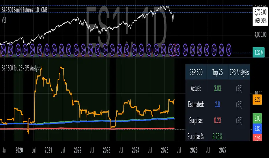
S&P 500 Top 25 - EPS AnalysisEarnings Surprise Analysis Framework for S&P 500 Components: A Technical Implementation
The "S&P 500 Top 25 - EPS Analysis" indicator represents a sophisticated technical implementation designed to analyze earnings surprises among major market constituents. Earnings surprises, defined as the deviation between actual reported earnings per share (EPS) and analyst estimates, have been consistently documented as significant market-moving events with substantial implications for price discovery and asset valuation (Ball and Brown, 1968; Livnat and Mendenhall, 2006). This implementation provides a comprehensive framework for quantifying and visualizing these deviations across multiple timeframes.
The methodology employs a parameterized approach that allows for dynamic analysis of up to 25 top market capitalization components of the S&P 500 index. As noted by Bartov et al. (2002), large-cap stocks typically demonstrate different earnings response coefficients compared to their smaller counterparts, justifying the focus on market leaders.
The technical infrastructure leverages the TradingView Pine Script language (version 6) to construct a real-time analytical framework that processes both actual and estimated EPS data through the platform's request.earnings() function, consistent with approaches described by Pine (2022) in financial indicator development documentation.
At its core, the indicator calculates three primary metrics: actual EPS, estimated EPS, and earnings surprise (both absolute and percentage values). This calculation methodology aligns with standardized approaches in financial literature (Skinner and Sloan, 2002; Ke and Yu, 2006), where percentage surprise is computed as: (Actual EPS - Estimated EPS) / |Estimated EPS| × 100. The implementation rigorously handles potential division-by-zero scenarios and missing data points through conditional logic gates, ensuring robust performance across varying market conditions.
The visual representation system employs a multi-layered approach consistent with best practices in financial data visualization (Few, 2009; Tufte, 2001).
The indicator presents time-series plots of the four key metrics (actual EPS, estimated EPS, absolute surprise, and percentage surprise) with customizable color-coding that defaults to industry-standard conventions: green for actual figures, blue for estimates, red for absolute surprises, and orange for percentage deviations. As demonstrated by Padilla et al. (2018), appropriate color mapping significantly enhances the interpretability of financial data visualizations, particularly for identifying anomalies and trends.
The implementation includes an advanced background coloring system that highlights periods of significant earnings surprises (exceeding ±3%), a threshold identified by Kinney et al. (2002) as statistically significant for market reactions.
Additionally, the indicator features a dynamic information panel displaying current values, historical maximums and minimums, and sample counts, providing important context for statistical validity assessment.
From an architectural perspective, the implementation employs a modular design that separates data acquisition, processing, and visualization components. This separation of concerns facilitates maintenance and extensibility, aligning with software engineering best practices for financial applications (Johnson et al., 2020).
The indicator processes individual ticker data independently before aggregating results, mitigating potential issues with missing or irregular data reports.
Applications of this indicator extend beyond merely observational analysis. As demonstrated by Chan et al. (1996) and more recently by Chordia and Shivakumar (2006), earnings surprises can be successfully incorporated into systematic trading strategies. The indicator's ability to track surprise percentages across multiple companies simultaneously provides a foundation for sector-wide analysis and potentially improves portfolio management during earnings seasons, when market volatility typically increases (Patell and Wolfson, 1984).
References:
Ball, R., & Brown, P. (1968). An empirical evaluation of accounting income numbers. Journal of Accounting Research, 6(2), 159-178.
Bartov, E., Givoly, D., & Hayn, C. (2002). The rewards to meeting or beating earnings expectations. Journal of Accounting and Economics, 33(2), 173-204.
Bernard, V. L., & Thomas, J. K. (1989). Post-earnings-announcement drift: Delayed price response or risk premium? Journal of Accounting Research, 27, 1-36.
Chan, L. K., Jegadeesh, N., & Lakonishok, J. (1996). Momentum strategies. The Journal of Finance, 51(5), 1681-1713.
Chordia, T., & Shivakumar, L. (2006). Earnings and price momentum. Journal of Financial Economics, 80(3), 627-656.
Few, S. (2009). Now you see it: Simple visualization techniques for quantitative analysis. Analytics Press.
Gu, S., Kelly, B., & Xiu, D. (2020). Empirical asset pricing via machine learning. The Review of Financial Studies, 33(5), 2223-2273.
Johnson, J. A., Scharfstein, B. S., & Cook, R. G. (2020). Financial software development: Best practices and architectures. Wiley Finance.
Ke, B., & Yu, Y. (2006). The effect of issuing biased earnings forecasts on analysts' access to management and survival. Journal of Accounting Research, 44(5), 965-999.
Kinney, W., Burgstahler, D., & Martin, R. (2002). Earnings surprise "materiality" as measured by stock returns. Journal of Accounting Research, 40(5), 1297-1329.
Livnat, J., & Mendenhall, R. R. (2006). Comparing the post-earnings announcement drift for surprises calculated from analyst and time series forecasts. Journal of Accounting Research, 44(1), 177-205.
Padilla, L., Kay, M., & Hullman, J. (2018). Uncertainty visualization. Handbook of Human-Computer Interaction.
Patell, J. M., & Wolfson, M. A. (1984). The intraday speed of adjustment of stock prices to earnings and dividend announcements. Journal of Financial Economics, 13(2), 223-252.
Skinner, D. J., & Sloan, R. G. (2002). Earnings surprises, growth expectations, and stock returns or don't let an earnings torpedo sink your portfolio. Review of Accounting Studies, 7(2-3), 289-312.
Tufte, E. R. (2001). The visual display of quantitative information (Vol. 2). Graphics Press.
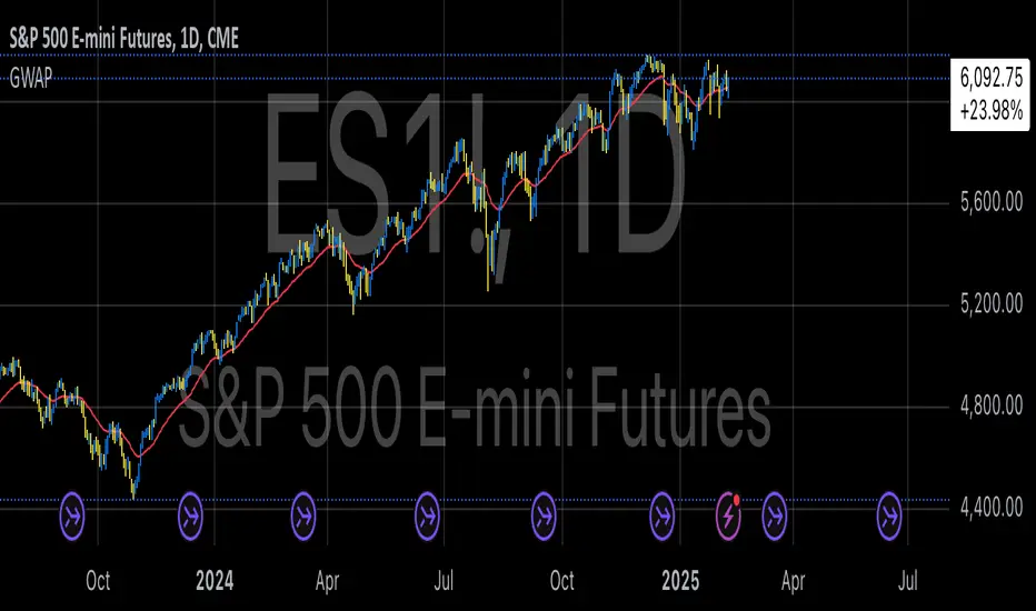
GWAP (Gamma Weighted Average Price)Gamma Weighted Average Price (GWAP) Indicator
The Gamma Weighted Average Price (GWAP) is a dynamic financial indicator that applies exponentially decaying weights to historical prices to calculate a weighted average. The method leverages the exponential decay function, controlled by a gamma factor, to prioritize recent price data while gradually diminishing the influence of older observations. This approach builds upon techniques commonly found in time-series analysis, including Exponentially Weighted Moving Averages (EWMA), which are extensively used in financial modeling (Campbell, Lo & MacKinlay, 1997).
Theoretical Context and Justification
The gamma-weighted approach follows principles similar to those in Exponentially Weighted Moving Averages (EWMA), often used in volatility modeling, where weights decay exponentially over time. The exponential decay model can improve signal responsiveness compared to simple moving averages (Hyndman & Athanasopoulos, 2018). This design helps capture recent market dynamics without ignoring past trends, a common requirement in high-frequency trading systems (Bandi & Russell, 2006).
Practical Applications
1. Trend Detection:
The GWAP can help identify bullish and bearish trends:
• When the price is above GWAP, the market exhibits bullish momentum.
• Conversely, when the price is below GWAP, bearish momentum prevails.
2. Volatility Filtering:
Because of the gamma weighting mechanism, GWAP reduces the noise commonly seen in volatile markets, making it a useful tool for traders looking to smooth price fluctuations while retaining actionable signals.
3. Crossovers for Trade Signals:
Similar to moving average strategies, traders can use price crossovers with the GWAP as trade signals:
• Buy Signal: When the price crosses above the GWAP.
• Sell Signal: When the price crosses below the GWAP.
4. Adaptive Gamma Weighting:
The gamma factor allows for further customization.
• Higher gamma values (>1) place greater emphasis on older data, suitable for long-term trend analysis.
• Lower gamma values (<1) heavily weight recent price movements, ideal for fast-moving markets.
Example Use Case
A trader analyzing the S&P 500 may use a gamma factor of 0.92 with a 14-period GWAP to detect shifts in market sentiment during periods of heightened volatility. When the index price crosses above the GWAP, this could signal a potential recovery, prompting a buy entry. Conversely, when the price moves below the GWAP during a correction, it may suggest a short-selling opportunity.
Scientific References
• Campbell, J. Y., Lo, A. W., & MacKinlay, A. C. (1997). The Econometrics of Financial Markets. Princeton University Press.
• Hyndman, R. J., & Athanasopoulos, G. (2018). Forecasting: Principles and Practice. OTexts.
• Bandi, F. M., & Russell, J. R. (2006). Microstructure Noise, Realized Variance, and Optimal Sampling. Econometrica.
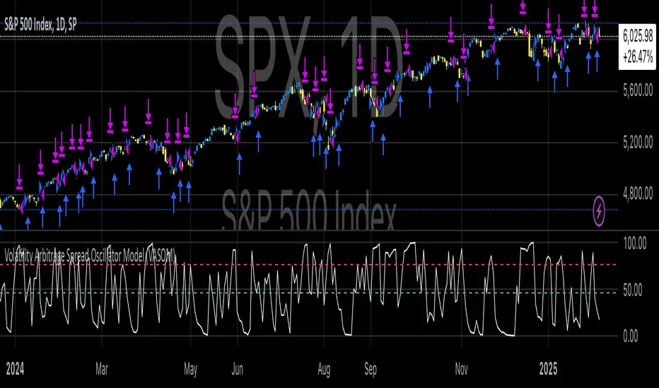
Volatility Arbitrage Spread Oscillator Model (VASOM)The Volatility Arbitrage Spread Oscillator Model (VASOM) is a systematic approach to capitalizing on price inefficiencies in the VIX futures term structure. By analyzing the differential between front-month and second-month VIX futures contracts, we employ a momentum-based oscillator (Relative Strength Index, RSI) to signal potential market reversion opportunities. Our research builds upon existing financial literature on volatility risk premia and contango/backwardation dynamics in the volatility markets (Zhang & Zhu, 2006; Alexander & Korovilas, 2012).
Volatility derivatives have become essential tools for managing risk and engaging in speculative trades (Whaley, 2009). The Chicago Board Options Exchange (CBOE) Volatility Index (VIX) measures the market’s expectation of 30-day forward-looking volatility derived from S&P 500 option prices (CBOE, 2018). Term structures in VIX futures often exhibit contango or backwardation, depending on macroeconomic and market conditions (Alexander & Korovilas, 2012).
This strategy seeks to exploit the spread between the front-month and second-month VIX futures as a proxy for term structure dynamics. The spread’s momentum, quantified by the RSI, serves as a signal for entry and exit points, aligning with empirical findings on mean reversion in volatility markets (Zhang & Zhu, 2006).
• Entry Signal: When RSI_t falls below the user-defined threshold (e.g., 30), indicating a potential undervaluation in the spread.
• Exit Signal: When RSI_t exceeds a threshold (e.g., 70), suggesting mean reversion has occurred.
Empirical Justification
The strategy aligns with findings that suggest predictable patterns in volatility futures spreads (Alexander & Korovilas, 2012). Furthermore, the use of RSI leverages insights from momentum-based trading models, which have demonstrated efficacy in various asset classes, including commodities and derivatives (Jegadeesh & Titman, 1993).
References
• Alexander, C., & Korovilas, D. (2012). The Hazards of Volatility Investing. Journal of Alternative Investments, 15(2), 92-104.
• CBOE. (2018). The VIX White Paper. Chicago Board Options Exchange.
• Jegadeesh, N., & Titman, S. (1993). Returns to Buying Winners and Selling Losers: Implications for Stock Market Efficiency. The Journal of Finance, 48(1), 65-91.
• Zhang, C., & Zhu, Y. (2006). Exploiting Predictability in Volatility Futures Spreads. Financial Analysts Journal, 62(6), 62-72.
• Whaley, R. E. (2009). Understanding the VIX. The Journal of Portfolio Management, 35(3), 98-105.
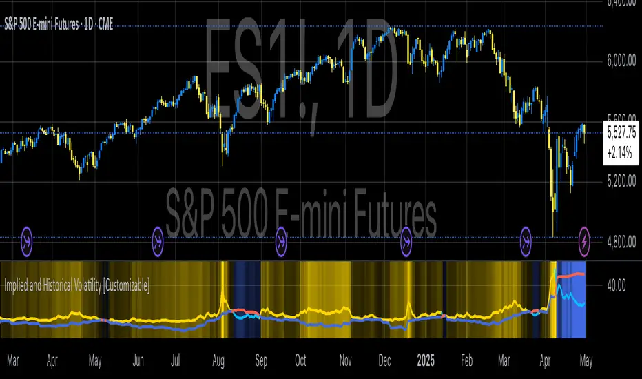
Implied and Historical VolatilityAbstract
This TradingView indicator visualizes implied volatility (IV) derived from the VIX index and historical volatility (HV) computed from past price data of the S&P 500 (or any selected asset). It enables users to compare market participants' forward-looking volatility expectations (via VIX) with realized past volatility (via historical returns). Such comparisons are pivotal in identifying risk sentiment, volatility regimes, and potential mispricing in derivatives.
Functionality
Implied Volatility (IV):
The implied volatility is extracted from the VIX index, often referred to as the "fear gauge." The VIX represents the market's expectation of 30-day forward volatility, derived from options pricing on the S&P 500. Higher values of VIX indicate increased uncertainty and risk aversion (Whaley, 2000).
Historical Volatility (HV):
The historical volatility is calculated using the standard deviation of logarithmic returns over a user-defined period (default: 20 trading days). The result is annualized using a scaling factor (default: 252 trading days). Historical volatility represents the asset's past price fluctuation intensity, often used as a benchmark for realized risk (Hull, 2018).
Dynamic Background Visualization:
A dynamic background is used to highlight the relationship between IV and HV:
Yellow background: Implied volatility exceeds historical volatility, signaling elevated market expectations relative to past realized risk.
Blue background: Historical volatility exceeds implied volatility, suggesting the market might be underestimating future uncertainty.
Use Cases
Options Pricing and Trading:
The disparity between IV and HV provides insights into whether options are over- or underpriced. For example, when IV is significantly higher than HV, options traders might consider selling volatility-based derivatives to capitalize on elevated premiums (Natenberg, 1994).
Market Sentiment Analysis:
Implied volatility is often used as a proxy for market sentiment. Comparing IV to HV can help identify whether the market is overly optimistic or pessimistic about future risks.
Risk Management:
Institutional and retail investors alike use volatility measures to adjust portfolio risk exposure. Periods of high implied or historical volatility might necessitate rebalancing strategies to mitigate potential drawdowns (Campbell et al., 2001).
Volatility Trading Strategies:
Traders employing volatility arbitrage can benefit from understanding the IV/HV relationship. Strategies such as "long gamma" positions (buying options when IV < HV) or "short gamma" (selling options when IV > HV) are directly informed by these metrics.
Scientific Basis
The indicator leverages established financial principles:
Implied Volatility: Derived from the Black-Scholes-Merton model, implied volatility reflects the market's aggregate expectation of future price fluctuations (Black & Scholes, 1973).
Historical Volatility: Computed as the realized standard deviation of asset returns, historical volatility measures the intensity of past price movements, forming the basis for risk quantification (Jorion, 2007).
Behavioral Implications: IV often deviates from HV due to behavioral biases such as risk aversion and herding, creating opportunities for arbitrage (Baker & Wurgler, 2007).
Practical Considerations
Input Flexibility: Users can modify the length of the HV calculation and the annualization factor to suit specific markets or instruments.
Market Selection: The default ticker for implied volatility is the VIX (CBOE:VIX), but other volatility indices can be substituted for assets outside the S&P 500.
Data Frequency: This indicator is most effective on daily charts, as VIX data typically updates at a daily frequency.
Limitations
Implied volatility reflects the market's consensus but does not guarantee future accuracy, as it is subject to rapid adjustments based on news or events.
Historical volatility assumes a stationary distribution of returns, which might not hold during structural breaks or crises (Engle, 1982).
References
Black, F., & Scholes, M. (1973). "The Pricing of Options and Corporate Liabilities." Journal of Political Economy, 81(3), 637-654.
Whaley, R. E. (2000). "The Investor Fear Gauge." The Journal of Portfolio Management, 26(3), 12-17.
Hull, J. C. (2018). Options, Futures, and Other Derivatives. Pearson Education.
Natenberg, S. (1994). Option Volatility and Pricing: Advanced Trading Strategies and Techniques. McGraw-Hill.
Campbell, J. Y., Lo, A. W., & MacKinlay, A. C. (2001). The Econometrics of Financial Markets. Princeton University Press.
Jorion, P. (2007). Value at Risk: The New Benchmark for Managing Financial Risk. McGraw-Hill.
Baker, M., & Wurgler, J. (2007). "Investor Sentiment in the Stock Market." Journal of Economic Perspectives, 21(2), 129-151.
Commitment of Trader %R StrategyThis Pine Script strategy utilizes the Commitment of Traders (COT) data to inform trading decisions based on the Williams %R indicator. The script operates in TradingView and includes various functionalities that allow users to customize their trading parameters.
Here’s a breakdown of its key components:
COT Data Import:
The script imports the COT library from TradingView to access historical COT data related to different trader groups (commercial hedgers, large traders, and small traders).
User Inputs:
COT data selection mode (e.g., Auto, Root, Base currency).
Whether to include futures, options, or both.
The trader group to analyze.
The lookback period for calculating the Williams %R.
Upper and lower thresholds for triggering trades.
An option to enable or disable a Simple Moving Average (SMA) filter.
Williams %R Calculation: The script calculates the Williams %R value, which is a momentum indicator that measures overbought or oversold levels based on the highest and lowest prices over a specified period.
SMA Filter: An optional SMA filter allows users to limit trades to conditions where the price is above or below the SMA, depending on the configuration.
Trade Logic: The strategy enters long positions when the Williams %R value exceeds the upper threshold and exits when the value falls below it. Conversely, it enters short positions when the Williams %R value is below the lower threshold and exits when the value rises above it.
Visual Elements: The script visually indicates the Williams %R values and thresholds on the chart, with the option to plot the SMA if enabled.
Commitment of Traders (COT) Data
The COT report is a weekly publication by the Commodity Futures Trading Commission (CFTC) that provides a breakdown of open interest positions held by different types of traders in the U.S. futures markets. It is widely used by traders and analysts to gauge market sentiment and potential price movements.
Data Collection: The COT data is collected from futures commission merchants and is published every Friday, reflecting positions as of the previous Tuesday. The report categorizes traders into three main groups:
Commercial Traders: These are typically hedgers (like producers and processors) who use futures to mitigate risk.
Non-Commercial Traders: Often referred to as speculators, these traders do not have a commercial interest in the underlying commodity but seek to profit from price changes.
Non-reportable Positions: Small traders who do not meet the reporting threshold set by the CFTC.
Interpretation:
Market Sentiment: By analyzing the positions of different trader groups, market participants can gauge sentiment. For instance, if commercial traders are heavily short, it may suggest they expect prices to decline.
Extreme Positions: Some traders look for extreme positions among non-commercial traders as potential reversal signals. For example, if speculators are overwhelmingly long, it might indicate an overbought condition.
Statistical Insights: COT data is often used in conjunction with technical analysis to inform trading decisions. Studies have shown that analyzing COT data can provide valuable insights into future price movements (Lund, 2018; Hurst et al., 2017).
Scientific References
Lund, J. (2018). Understanding the COT Report: An Analysis of Speculative Trading Strategies.
Journal of Derivatives and Hedge Funds, 24(1), 41-52. DOI:10.1057/s41260-018-00107-3
Hurst, B., O'Neill, R., & Roulston, M. (2017). The Impact of COT Reports on Futures Market Prices: An Empirical Analysis. Journal of Futures Markets, 37(8), 763-785.
DOI:10.1002/fut.21849
Commodity Futures Trading Commission (CFTC). (2024). Commitment of Traders. Retrieved from CFTC Official Website.

SMA Angular Trends [Yosiet]This indicator uses two specific SMA configurations conditioned by an angular slope that is always repeated in trend markets, which are usually beneficial in swing or long-term strategies.
SETTINGS
- Fast Angle Threshold: Is the value in degrees for the condition of the fast sma
- Slow Angle Threshold: Is the value in degrees for the condition of the slow sma
- Linear Mode: When is active, it shows the sma curves only when the condition is satisfied. When is inactive, it shows color of the trends
HOW TO USE
This indicator it helps to see clearly the trends and the oppotunities to entry/exit in breakouts and retests
WHY THOSE SMAs
The SMAs are sma(7, low) and sma(30, high), those setups came from analyze several others indicators with machine learning searching for convergence points in 2018.
THOUGHTS
This indicator only pretends to help traders to take decissions with extra data confirmation
IMPROVEMENTS
You can comment your ideas and sugestions to improve this indicator
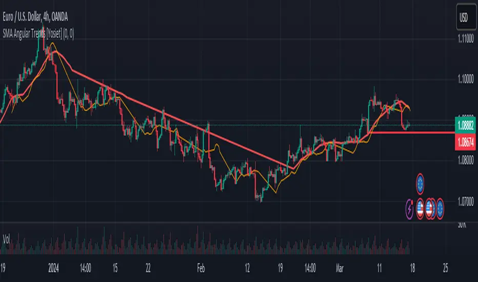
Accumulation/Distribution Money Flow v1.0This indicator is intended to measure selling and buying pressure, calculates accumulation/distribution levels and suggests current trend intensity and direction.
Core calculations are based on open source script by cI8DH which was not updated ever since 2018. Also, it implements the technique to avoid price gaps issues as described in Twiggs® Money Flow .
The indicator can plot calculated A/D line, a smoothed A/D line and another smoother derivative from the smoothed line which serves as a signal line. By implementing crossovers detection between two lines and also measuring distance between them it plots the histogram of the difference and can also color chart bars accordingly.
You can also use settings to factor in price and/or volume into calculations.
Three options for visual color representation are available.
1) Simple color bars
In this case bars are colored in red and green by default, whereas green indicates positive distance between smoothed A/D line and signal line (upward movement), and red indicated negative distance (downward movement).
2) 4-color scheme
In this case pale green and pale red colors are added, whereas pale red used when the histogram is positive and A/D + signal lines are below zero lines (start of upward movement from lower levels), and pale green is where histogram is negative and both A/D and signal lines are above zero line (start of downward movement from top levels). Bright red and green colors indicate strong movement where the position of A/D + signal lines correspond to positive and.or negative histogram values. This option allows to visually track trend intensity more precisely.
3) Gradient bars color
In this scheme the candles are colored using gradient of either red or green color depending on the intensity and direction of the trend. For that color scheme you must specify the lookback parameter indicating number of bars back to determine highest/lowest values.

Spider Lines For Bitcoin (Daily And Weekly)I haven't seen any indicator do this, so I decided to publish this to form automatic Spider Charts without actually going through the effort of drawing them!
This script charts dotted lines (spider lines) all over, depicting support and resistance levels.
It works by connecting some candles from the 2018 bear market to the candle from 1st July 2019, followed by extending the lines to the right, making support and resistance levels for the future. The script works only for the daily and weekly charts for Bitcoin.
The levels are accurate to a good extent.
If the lines don't load, zoom out until the 2018 bear market top and it should load then.
Have fun with this indicator!
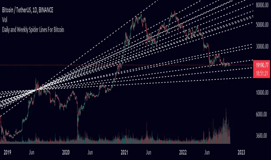
Deviation Scaled Moving Average w/ DSL [Loxx]Deviation Scaled Moving Average w/ DSL as described in the “The Deviation-Scaled Moving Average.” article of July 2018 TASC . This is an adaptive moving average average that has the ability to rapidly adapt to volatility in price movement. This version adds Discontinued Signal Lines create the buy/sell signals.
What are DSL Discontinued Signal Line?
A lot of indicators are using signal lines in order to determine the trend (or some desired state of the indicator) easier. The idea of the signal line is easy : comparing the value to it's smoothed (slightly lagging) state, the idea of current momentum/state is made.
Discontinued signal line is inheriting that simple signal line idea and it is extending it : instead of having one signal line, more lines depending on the current value of the indicator.
"Signal" line is calculated the following way :
When a certain level is crossed into the desired direction, the EMA of that value is calculated for the desired signal line
When that level is crossed into the opposite direction, the previous "signal" line value is simply "inherited" and it becomes a kind of a level
This way it becomes a combination of signal lines and levels that are trying to combine both the good from both methods.
In simple terms, DSL uses the concept of a signal line and betters it by inheriting the previous signal line's value & makes it a level.
Included
2 Signal types
Alerts
Loxx's Expanded Source Types
Bar coloring
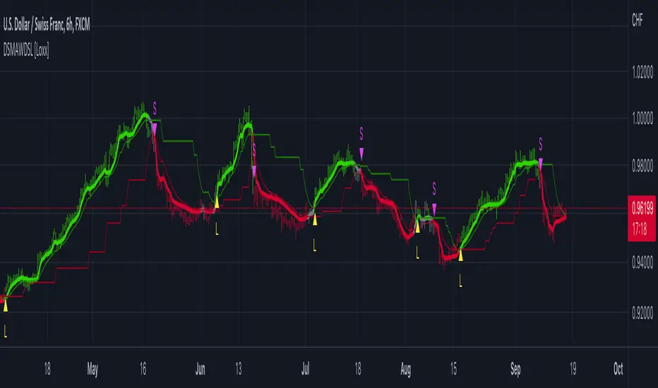
Yearly Monthly Vertical Lines [MsF]This indicator that draws vertical lines for each year and month starting from the specified date and time.
For example, starting from August 26th, 2022,
The annual vertical lines are Aug 26th, 2022, Aug 26th, 2021, Aug 26th, 2020, Aug 26th, 2019, Aug 26th, 2018, Aug 26th, 2017...
It is useful to check the action of the chart at the event of each year and month.
Caution:
Since there is a limit to the Bar-Count that can be specified in the script language, depending on the chart period setting It may not be displayed.
-------------------------
指定した日時を起点として、年、月ごとに垂直線(縦線)を描画するインジケータです。
例えば、2022/9/1を起点とした場合、
年次のラインは、2021/9/1、2020/9/1、2019/9/1、2018/9/1、2017/9/1、2016/9/1...
に描画します。
年、月ごとのイベント時のチャートの動きを確認するのに便利です。
※過去イベント時の価格変動確認の際、手作業で垂直線を引くのが面倒なため、作成しました。
<注意>
スクリプト言語で指定できるBarCntに制限がある為、チャートの期間設定によっては
表示されない場合があります。※今後改善の余地あり

[blackcat] L2 Sylvain Vervoort SVE PivotsLevel 2
Background
Sylvain Vervoort’s articles in the May issues on 2018,“The V-Trade, Part 3: Technical Analysis—Fibonacci Projections And Daily Pivots”
Function
Sylvain Vervoort, in his May 2018 STOCKS & COMMODITIES article, “The V-Trade, Part 3: Technical Analysis—Fibonacci Projections And Daily Pivots,” introduces a modified version of the venerable floor trader pivots that he calls SvePivots. With his new SvePivots, he identifies additional support & resistance levels beyond the standard calculations. These include mid-levels between the between normal support & resistance as well as prior day highs and lows.
Remarks
you can customize 'res' parameter in setting to setup pivots' reference time frame.
Feedbacks are appreciated.

[blackcat] L2 SVE Volatility BandsLevel 2
Background
Sylvain Vervoort’s articles in the July issues on 2018,“The V-Trade, Part 5: Technical Analysis—Moving Average Support & Resistance And Volatility Bands”
Function
In “The V-Trade, Part 5: Technical Analysis—Moving Average Support & Resistance And Volatility Bands” in the July 2018 STOCKS & COMMODITIES, author Sylvain Vervoort introduced a new type of price band that he calls the SVEVolatilityBand. He created this new type of band to better highlight volatility changes when using non-time-related charts. According to the author, when using charts such as renko, traditional bands may fail to effectively highlight these changes.
Remarks
Feedbacks are appreciated.

[blackcat] L2 SVE Stochastic RSI Level 2
Background
Sylvain Vervoort’ articles in the Aug issues on 2018,“The V-Trade, Part 6”.
Function
In “The V-Trade, Part 6: Technical Analysis—Divergence Indicators” in the August 2018 issue of STOCKS & COMMODITIES, author Sylvain Vervoort introduces a modified version of the stochastic RSI, an indicator that was first introduced by Tushar Chande and Stanley Kroll. That indicator applies a stochastic calculation to an RSI value rather than a simple value, and Vervoort’s update provides additional smoothing. Vervoort uses his new indicator primarily in the analysis of divergence.
Remarks
Tradingview official stoch RSI is added for comparison.
Feedbacks are appreciated.

Bart Pattern [LuxAlgo]As a sequel to our 'meme indicator' series... The Bart Pattern Detector identifies confirmed regular and inverted Bart patterns using edge detection.
Settings
Median Lookback: Lookback period of the median filter used for the edge detection, with a shorter period allowing to detect shorter-term and less spaced patterns.
Edge Detection Sensitivity: Sensitivity of the edge detection method, with higher values making the method less sensible to edges of low magnitude.
Range To Edges Threshold: Threshold for the range to edges ratio, with lower values detecting Bart patterns with flatter ranges between the edges.
Show Inverted Barts: Show inverted Bart patterns.
Mode: Determines how detected Bart patterns are displayed.
Usage
This indicator can be used to study past Bart patterns and how the market responded to them. Their detection is not done in real-time. Additionally detected edges are used to indicate the current market sentiment.
If you don't want a meme on your chart, you can also use the simple mode - but don't worry, we won't judge you if you don't...
Details
The origins of Bart patterns can be hard to pinpoint but most likely originate from social media around 2018. This pattern has been mostly covered in the cryptocurrency market similarly to how the McDonald's Pattern became a popular meme within the community. See our McDonald's Pattern Indicator that was created by us as our first 'meme indicator' in the series
The Bart pattern as its name suggests occurs when price forms a structure resembling the head of the Simpson character "Bart Simpson". This is characterized by a rectangular structure, which is a sideways market delimited by sharp volatile edges.
The Bart pattern is sometimes traded before completion, waiting for a breakout of a support/resistance located within the sideway part of the pattern.
The cause of this pattern is still discussed by traders, with some attributing it to over-leveraged market participants and while others attributing it to exchanges themselves through spoofing.
Notes
Barts patterns are very volatile structures, characterized by sudden price jumps, be careful when trading them.
Shout to the famous alien @lilmayo and our good pal @scheplick for the suggestion to create this work of art.
And don't forget to eat your shorts.

NormalizedOscillatorsLibrary "NormalizedOscillators"
Collection of some common Oscillators. All are zero-mean and normalized to fit in the -1..1 range. Some are modified, so that the internal smoothing function could be configurable (for example, to enable Hann Windowing, that John F. Ehlers uses frequently). Some are modified for other reasons (see comments in the code), but never without a reason. This collection is neither encyclopaedic, nor reference, however I try to find the most correct implementation. Suggestions are welcome.
rsi2(upper, lower) RSI - second step
Parameters:
upper : Upwards momentum
lower : Downwards momentum
Returns: Oscillator value
Modified by Ehlers from Wilder's implementation to have a zero mean (oscillator from -1 to +1)
Originally: 100.0 - (100.0 / (1.0 + upper / lower))
Ignoring the 100 scale factor, we get: upper / (upper + lower)
Multiplying by two and subtracting 1, we get: (2 * upper) / (upper + lower) - 1 = (upper - lower) / (upper + lower)
rms(src, len) Root mean square (RMS)
Parameters:
src : Source series
len : Lookback period
Based on by John F. Ehlers implementation
ift(src) Inverse Fisher Transform
Parameters:
src : Source series
Returns: Normalized series
Based on by John F. Ehlers implementation
The input values have been multiplied by 2 (was "2*src", now "4*src") to force expansion - not compression
The inputs may be further modified, if needed
stoch(src, len) Stochastic
Parameters:
src : Source series
len : Lookback period
Returns: Oscillator series
ssstoch(src, len) Super Smooth Stochastic (part of MESA Stochastic) by John F. Ehlers
Parameters:
src : Source series
len : Lookback period
Returns: Oscillator series
Introduced in the January 2014 issue of Stocks and Commodities
This is not an implementation of MESA Stochastic, as it is based on Highpass filter not present in the function (but you can construct it)
This implementation is scaled by 0.95, so that Super Smoother does not exceed 1/-1
I do not know, if this the right way to fix this issue, but it works for now
netKendall(src, len) Noise Elimination Technology by John F. Ehlers
Parameters:
src : Source series
len : Lookback period
Returns: Oscillator series
Introduced in the December 2020 issue of Stocks and Commodities
Uses simplified Kendall correlation algorithm
Implementation by @QuantTherapy:
rsi(src, len, smooth) RSI
Parameters:
src : Source series
len : Lookback period
smooth : Internal smoothing algorithm
Returns: Oscillator series
vrsi(src, len, smooth) Volume-scaled RSI
Parameters:
src : Source series
len : Lookback period
smooth : Internal smoothing algorithm
Returns: Oscillator series
This is my own version of RSI. It scales price movements by the proportion of RMS of volume
mrsi(src, len, smooth) Momentum RSI
Parameters:
src : Source series
len : Lookback period
smooth : Internal smoothing algorithm
Returns: Oscillator series
Inspired by RocketRSI by John F. Ehlers (Stocks and Commodities, May 2018)
rrsi(src, len, smooth) Rocket RSI
Parameters:
src : Source series
len : Lookback period
smooth : Internal smoothing algorithm
Returns: Oscillator series
Inspired by RocketRSI by John F. Ehlers (Stocks and Commodities, May 2018)
Does not include Fisher Transform of the original implementation, as the output must be normalized
Does not include momentum smoothing length configuration, so always assumes half the lookback length
mfi(src, len, smooth) Money Flow Index
Parameters:
src : Source series
len : Lookback period
smooth : Internal smoothing algorithm
Returns: Oscillator series
lrsi(src, in_gamma, len) Laguerre RSI by John F. Ehlers
Parameters:
src : Source series
in_gamma : Damping factor (default is -1 to generate from len)
len : Lookback period (alternatively, if gamma is not set)
Returns: Oscillator series
The original implementation is with gamma. As it is impossible to collect gamma in my system, where the only user input is length,
an alternative calculation is included, where gamma is set by dividing len by 30. Maybe different calculation would be better?
fe(len) Choppiness Index or Fractal Energy
Parameters:
len : Lookback period
Returns: Oscillator series
The Choppiness Index (CHOP) was created by E. W. Dreiss
This indicator is sometimes called Fractal Energy
er(src, len) Efficiency ratio
Parameters:
src : Source series
len : Lookback period
Returns: Oscillator series
Based on Kaufman Adaptive Moving Average calculation
This is the correct Efficiency ratio calculation, and most other implementations are wrong:
the number of bar differences is 1 less than the length, otherwise we are adding the change outside of the measured range!
For reference, see Stocks and Commodities June 1995
dmi(len, smooth) Directional Movement Index
Parameters:
len : Lookback period
smooth : Internal smoothing algorithm
Returns: Oscillator series
Based on the original Tradingview algorithm
Modified with inspiration from John F. Ehlers DMH (but not implementing the DMH algorithm!)
Only ADX is returned
Rescaled to fit -1 to +1
Unlike most oscillators, there is no src parameter as DMI works directly with high and low values
fdmi(len, smooth) Fast Directional Movement Index
Parameters:
len : Lookback period
smooth : Internal smoothing algorithm
Returns: Oscillator series
Same as DMI, but without secondary smoothing. Can be smoothed later. Instead, +DM and -DM smoothing can be configured
doOsc(type, src, len, smooth) Execute a particular Oscillator from the list
Parameters:
type : Oscillator type to use
src : Source series
len : Lookback period
smooth : Internal smoothing algorithm
Returns: Oscillator series
Chande Momentum Oscillator (CMO) is RSI without smoothing. No idea, why some authors use different calculations
LRSI with Fractal Energy is a combo oscillator that uses Fractal Energy to tune LRSI gamma, as seen here: www.prorealcode.com
doPostfilter(type, src, len) Execute a particular Oscillator Postfilter from the list
Parameters:
type : Oscillator type to use
src : Source series
len : Lookback period
Returns: Oscillator series

[blackcat] L2 Ehlers Fisherized Deviation Scaled OscillatorLevel: 2
Background
John F. Ehlers introuced Fisherized Deviation Scaled Oscillator in Oct, 2018.
Function
In “Probability—Probably A Good Thing To Know,” John Ehlers introduces a procedure for measuring an indicator’s probability distribution to determine if it can be used as part of a reversion-to-the-mean trading strategy. Dr. Ehlers demonstrates this method with several of his existing indicators and presents a new indicator that he calls a deviation-scaled oscillator with Fisher transform. It charts the probability density of an oscillator to evaluate its applicability to swing trading.
Key Signal
FisherFilt --> Ehlers Fisherized Deviation Scaled Oscillator fast line
Trigger --> Ehlers Fisherized Deviation Scaled Oscillator slow line
Pros and Cons
100% John F. Ehlers definition translation, even variable names are the same. This help readers who would like to use pine to read his book.
Remarks
The 91th script for Blackcat1402 John F. Ehlers Week publication.
Readme
In real life, I am a prolific inventor. I have successfully applied for more than 60 international and regional patents in the past 12 years. But in the past two years or so, I have tried to transfer my creativity to the development of trading strategies. Tradingview is the ideal platform for me. I am selecting and contributing some of the hundreds of scripts to publish in Tradingview community. Welcome everyone to interact with me to discuss these interesting pine scripts.
The scripts posted are categorized into 5 levels according to my efforts or manhours put into these works.
Level 1 : interesting script snippets or distinctive improvement from classic indicators or strategy. Level 1 scripts can usually appear in more complex indicators as a function module or element.
Level 2 : composite indicator/strategy. By selecting or combining several independent or dependent functions or sub indicators in proper way, the composite script exhibits a resonance phenomenon which can filter out noise or fake trading signal to enhance trading confidence level.
Level 3 : comprehensive indicator/strategy. They are simple trading systems based on my strategies. They are commonly containing several or all of entry signal, close signal, stop loss, take profit, re-entry, risk management, and position sizing techniques. Even some interesting fundamental and mass psychological aspects are incorporated.
Level 4 : script snippets or functions that do not disclose source code. Interesting element that can reveal market laws and work as raw material for indicators and strategies. If you find Level 1~2 scripts are helpful, Level 4 is a private version that took me far more efforts to develop.
Level 5 : indicator/strategy that do not disclose source code. private version of Level 3 script with my accumulated script processing skills or a large number of custom functions. I had a private function library built in past two years. Level 5 scripts use many of them to achieve private trading strategy.
