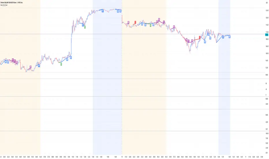
Stoch_RSI_ChartEnhanced Stochastic RSI Divergence Indicator with VWAP Filter for Charts
This custom indicator builds upon the classic Stochastic RSI to automatically detect both regular and hidden divergences. It’s designed to help traders spot potential market reversals or continuations using two methods for divergence detection (fractal‑ and pivot‑based) while offering optional VWAP filtering for confirmation.
Key Features
Stoch RSI Calculation
The indicator computes a smoothed Stoch RSI using configurable parameters for RSI length, stochastic length, and smoothing periods. An option to average the K and D lines provides a cleaner momentum view.
Divergence Detection via Fractals & Pivots
Fractal-Based Divergences:
Looks for 4-candle patterns to identify higher-highs or lower-lows in the price that are not confirmed by the oscillator, signaling potential reversals.
Pivot-Based Divergences:
Utilizes TradingView’s built-in pivot functions to find divergence conditions over adjustable pivot ranges.
Regular vs. Hidden Divergences:
Regular Divergence: Occurs when price makes a new extreme (higher high or lower low) while the Stoch RSI fails to follow suit.
Hidden Divergence: Indicates potential trend continuations when the oscillator diverges against the established price trend.
Optional VWAP Filtering
The script includes two optional VWAP filters that work as follows:
VWAP Filter on Regular Divergences:
Only confirms regular divergence signals if the current price satisfies the VWAP condition (e.g., price is above VWAP for bullish signals, below VWAP for bearish signals).
VWAP Filter on Hidden Divergences:
Similarly, hidden divergence signals are validated only when the price meets specific VWAP conditions, adding an extra layer of trend confirmation.
Customizable Alerts and Visual Labels
Easily configure divergence labels (“B” for bullish, “S” for bearish) and enable up to four alert conditions for real‑time notifications when a divergence occurs.
Credits & History:
Log RSI by @fskrypt
Divergence Detection originally by @RicardoSantos (with edits from @JustUncleL)
Further Edits by @NeoButane on August 8, 2018
Latest Edits by @FYMD on June 1, 2024
Cerca negli script per "米哈游2018年股票价格"
(US) Historical Trade WarsHistorical U.S. Trade Wars Indicator
Overview
This indicator visualizes major U.S. trade wars and disputes throughout modern economic history, from the McKinley Tariff of 1890 to recent U.S.-China tensions. This U.S.-focused timeline is perfect for macro traders, economic historians, and anyone looking to understand how America's trade conflicts correlate with market movements.
Features
Comprehensive U.S. Timeline: Covers 130+ years of U.S.-centered trade disputes with historically accurate dates.
Color-Coded Events:
🔴 Red: Marks the beginning of a U.S. trade war or major dispute.
🟡 Yellow: Highlights significant events within a trade conflict.
🟢 Green: Shows resolutions or ends of trade disputes.
Global Partners/Rivals: Tracks U.S. trade relations with China, Japan, EU, Canada, Mexico, Brazil, Argentina, and others.
Country Flags: Uses emoji flags for easy visual identification of nations in trade relations with the U.S.
Major Trade Wars Covered:
McKinley Tariff (1890-1894)
Smoot-Hawley Tariff Act (1930-1934)
U.S.-Europe Chicken War (1962-1974)
Multifiber Arrangement Quotas (1974-2005)
Japan-U.S. Trade Disputes (1981-1989)
NAFTA and Softwood Lumber Disputes
Clinton and Bush-Era Steel Tariffs
Obama-Era China Tire Tariffs
Rare Earth Minerals Dispute (2012-2014)
Solar Panel Dispute (2012-2015)
TPP and TTIP Negotiations
U.S.-China Trade War (2018-present)
Airbus-Boeing Dispute
Usage
Analyze how markets historically responded to trade war initiations and resolutions.
Identify patterns in market behavior during periods of trade tensions.
Use as an overlay with price action to examine correlations.
Perfect companion for macro analysis on daily, weekly, or monthly charts.
About
This indicator is designed as a historical reference tool for traders and economic analysts focusing on U.S. trade policy and its global impact. The dates and events have been thoroughly researched for accuracy. Each label includes emojis to indicate the U.S. and its trade partners/rivals, making it easy to track America's evolving trade relationships across time.
Note: This indicator works best on larger timeframes (daily, weekly, monthly) due to the historical span covered.

KalmanfilterLibrary "Kalmanfilter"
A sophisticated Kalman Filter implementation for financial time series analysis
@author Rocky-Studio
@version 1.0
initialize(initial_value, process_noise, measurement_noise)
Initializes Kalman Filter parameters
Parameters:
initial_value (float) : (float) The initial state estimate
process_noise (float) : (float) The process noise coefficient (Q)
measurement_noise (float) : (float) The measurement noise coefficient (R)
Returns: A tuple containing
update(prev_state, prev_covariance, measurement, process_noise, measurement_noise)
Update Kalman Filter state
Parameters:
prev_state (float)
prev_covariance (float)
measurement (float)
process_noise (float)
measurement_noise (float)
calculate_measurement_noise(price_series, length)
Adaptive measurement noise calculation
Parameters:
price_series (array)
length (int)
calculate_measurement_noise_simple(price_series)
Parameters:
price_series (array)
update_trading(prev_state, prev_velocity, prev_covariance, measurement, volatility_window)
Enhanced trading update with velocity
Parameters:
prev_state (float)
prev_velocity (float)
prev_covariance (float)
measurement (float)
volatility_window (int)
model4_update(prev_mean, prev_speed, prev_covariance, price, process_noise, measurement_noise)
Kalman Filter Model 4 implementation (Benhamou 2018)
Parameters:
prev_mean (float)
prev_speed (float)
prev_covariance (array)
price (float)
process_noise (array)
measurement_noise (float)
model4_initialize(initial_price)
Initialize Model 4 parameters
Parameters:
initial_price (float)
model4_default_process_noise()
Create default process noise matrix for Model 4
model4_calculate_measurement_noise(price_series, length)
Adaptive measurement noise calculation for Model 4
Parameters:
price_series (array)
length (int)

BTC Seasonality Strategy (Weekly)This strategy identifies potential weekend opportunities in Bitcoin (BTC) markets by leveraging the concept of seasonality, entering a position at a predefined time and day, and exiting at a specified time and day.
Key Features
Customizable Time and Day Selection:
Users can select the entry and exit days and corresponding times (in EST).
Directional Flexibility:
The strategy allows traders to choose between long or short positions.
TradingView Compliance:
The script adheres to TradingView's house rules, avoids overly complex conditions, and provides clear user-configurable inputs.
How It Works
The script determines the current weekday and hour in EST, converting TradingView's UTC time for accurate comparisons.
If the current day and hour match the selected entry conditions, a trade (long or short) is opened.
The position is closed when the current day and hour match the specified exit conditions.
Theoretical Basis
Market Seasonality:
The concept of seasonality in financial markets refers to predictable patterns based on time, such as weekends or specific days of the week. Studies have shown that cryptocurrency markets exhibit unique trading behaviors during weekends due to reduced institutional activity and higher retail participation behavioral Biases**:
Retail traders often dominate weekend markets, potentially causing predictable inefficiencies .
Reverences**
Baur, D. G., Hong, K., & Lee, A. D. (2018). Bitcoin: Medium of exchange or speculative assets? Journal of International Financial Markets, Institutions and Money, 54, 177–189.
Urquhart, A. (2016). The inefficiency of Bitcoin. Economics Letters, 148, 80–82.

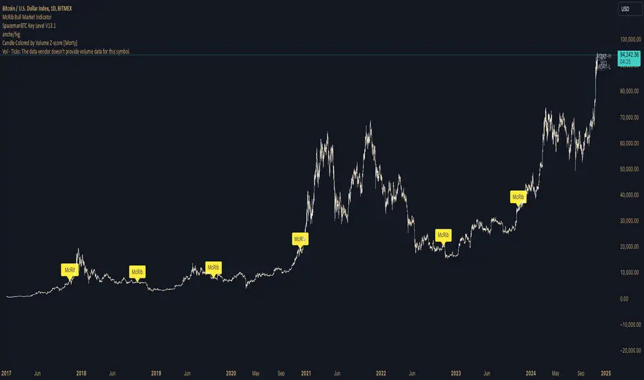
McRib Bull Market Indicator# McRib Bull Market Indicator
## Overview
The McRib Bull Market Indicator is a unique technical analysis tool that marks McDonald's McRib sandwich release dates on your trading charts. While seemingly unconventional, this indicator serves as a fascinating historical reference point for market analysis, particularly for studying periods of market expansion.
## Key Features
- Visual yellow labels marking verified McRib release dates from 2012 to 2024
- Clean, unobtrusive design that overlays on any chart timeframe
- Covers both U.S. and international releases (including UK and Australia)
## Historical Reference Points
The indicator includes release dates from:
- December 2012
- October-December 2014
- January 2015
- October 2016
- November 2017
- October 2018
- October 2019
- December 2020
- October 2022
- November 2023
- December 2024
## Usage Guide
1. Add the indicator to any chart by searching for "McRib Bull Market Indicator"
2. The indicator will automatically display yellow labels above price candles on McRib release dates
3. Use these reference points to:
- Analyze market conditions during McRib releases
- Study potential correlations between releases and market movements
- Compare market behavior across different McRib release periods
- Identify any patterns in market expansion phases coinciding with releases
## Trading Application
While initially created as a novelty indicator, it can be used to:
- Mark specific historical points of reference for broader market analysis
- Study potential market psychology around major promotional events
- Compare seasonal market patterns with recurring release dates
- Analyze market expansion phases that coincide with releases
Remember: While this indicator provides interesting historical reference points, it should be used as part of a comprehensive trading strategy rather than as a standalone trading signal.
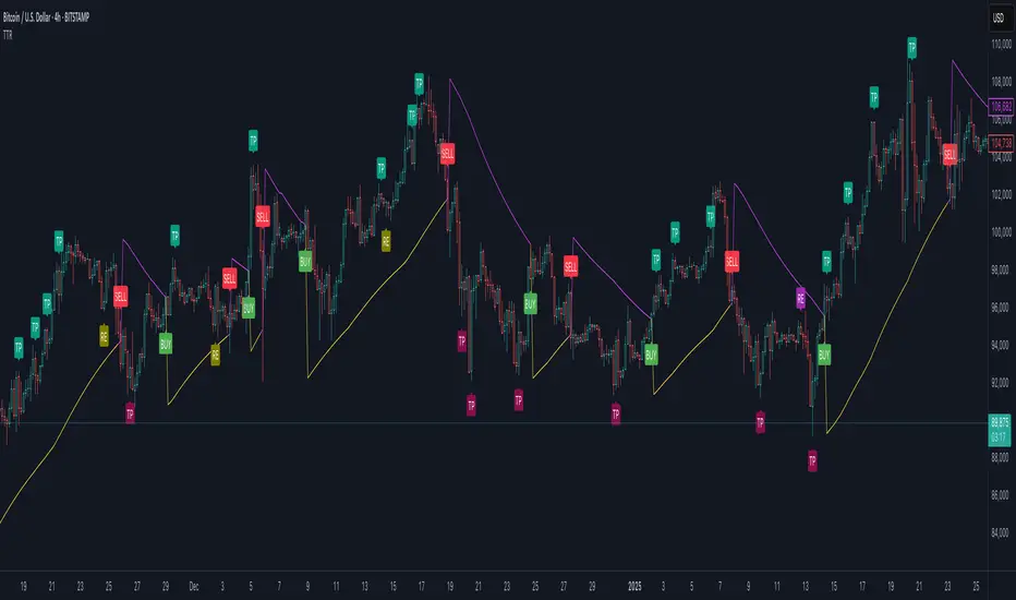
Trend Trader-RemasteredThe script was originally coded in 2018 with Pine Script version 3, and it was in invite only status. It has been updated and optimised for Pine Script v5 and made completely open source.
Overview
The Trend Trader-Remastered is a refined and highly sophisticated implementation of the Parabolic SAR designed to create strategic buy and sell entry signals, alongside precision take profit and re-entry signals based on marked Bill Williams (BW) fractals. Built with a deep emphasis on clarity and accuracy, this indicator ensures that only relevant and meaningful signals are generated, eliminating any unnecessary entries or exits.
Key Features
1) Parabolic SAR-Based Entry Signals:
This indicator leverages an advanced implementation of the Parabolic SAR to create clear buy and sell position entry signals.
The Parabolic SAR detects potential trend shifts, helping traders make timely entries in trending markets.
These entries are strategically aligned to maximise trend-following opportunities and minimise whipsaw trades, providing an effective approach for trend traders.
2) Take Profit and Re-Entry Signals with BW Fractals:
The indicator goes beyond simple entry and exit signals by integrating BW Fractal-based take profit and re-entry signals.
Relevant Signal Generation: The indicator maintains strict criteria for signal relevance, ensuring that a re-entry signal is only generated if there has been a preceding take profit signal in the respective position. This prevents any misleading or premature re-entry signals.
Progressive Take Profit Signals: The script generates multiple take profit signals sequentially in alignment with prior take profit levels. For instance, in a buy position initiated at a price of 100, the first take profit might occur at 110. Any subsequent take profit signals will then occur at prices greater than 110, ensuring they are "in favour" of the original position's trajectory and previous take profits.
3) Consistent Trend-Following Structure:
This design allows the Trend Trader-Remastered to continue signaling take profit opportunities as the trend advances. The indicator only generates take profit signals in alignment with previous ones, supporting a systematic and profit-maximising strategy.
This structure helps traders maintain positions effectively, securing incremental profits as the trend progresses.
4) Customisability and Usability:
Adjustable Parameters: Users can configure key settings, including sensitivity to the Parabolic SAR and fractal identification. This allows flexibility to fine-tune the indicator according to different market conditions or trading styles.
User-Friendly Alerts: The indicator provides clear visual signals on the chart, along with optional alerts to notify traders of new buy, sell, take profit, or re-entry opportunities in real-time.
Formation Defined Moving Support and ResistanceThe script was originally coded in 2018 with Pine Script version 3, and it was in protected code status. It has been updated and optimised for Pine Script v5 and made completely open source.
The Formation Defined Moving Support and Resistance indicator is a sophisticated tool for identifying dynamic support and resistance levels based on specific price formations and level interactions. This indicator goes beyond traditional static support and resistance by updating levels based on predefined formation patterns and market behaviour, providing traders with a more responsive view of potential support and resistance zones.
Features:
The indicator detects essential price levels:
Lower Low (LL)
Higher Low (HL)
Higher High (HH)
Lower High (LH)
Equal Lower Low (ELL)
Equal Higher Low (EHL)
Equal Higher High (EHH)
Equal Lower High (ELH)
By identifying these key points, the script builds a foundation for tracking and responding to changes in price structure.
Pre-defined Formations and Comparisons:
The indicator calculates and recognises nine different pre-defined formations, such as bullish and bearish formations, based on the sequence of price levels.
These formations are compared against previous levels and formations, allowing for a sophisticated understanding of recent market movements and momentum shifts.
This formation-based approach provides insights into whether the price is likely to maintain, break, or reverse key levels.
Dynamic Support and Resistance Levels:
The indicator offers an option to toggle Moving Support and Resistance Levels.
When enabled, the support and resistance levels dynamically adjust:
Upon a change in the detected formation.
When the bar’s closing price breaks the last defined support or resistance level.
This feature ensures that the support and resistance levels adapt quickly to market changes, giving a more accurate and responsive perspective.
Customisable Price Source:
Users can choose the price source for level detection, selecting between close or high/low prices.
This flexibility allows the indicator to adapt to different trading styles, whether the focus is on closing prices for more conservative levels or on highs and lows for more sensitive level tracking.
This indicator can benefit traders relying on dynamic support and resistance rather than fixed, historical levels. It adapts to recent price actions and market formations, making it useful for identifying entry and exit points, trend continuation or reversal, and setting trailing stops based on updated support and resistance levels.

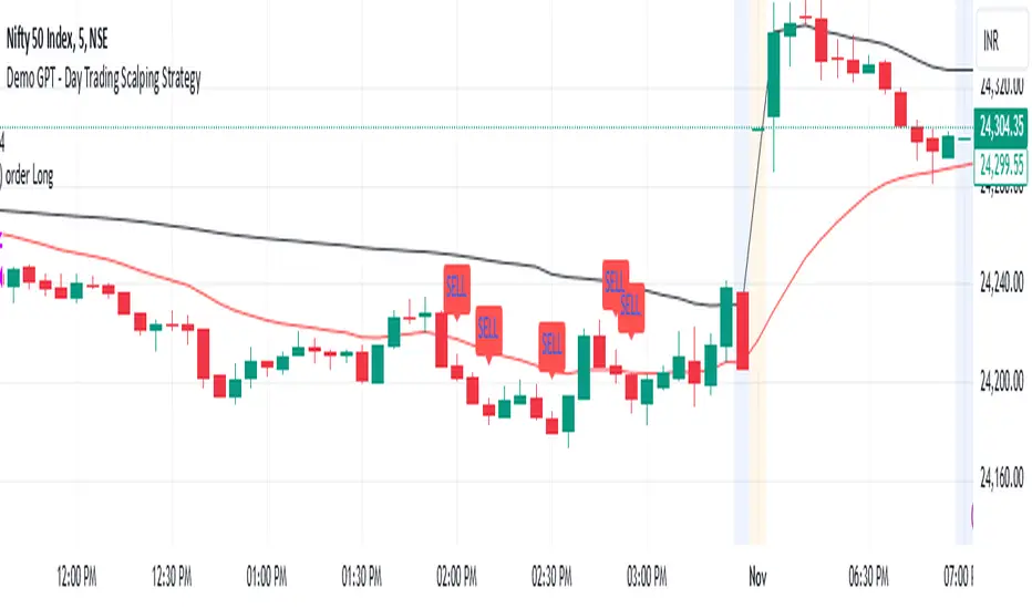
Demo GPT - Day Trading Scalping StrategyOverview:
This strategy is designed for day trading and scalping, utilizing a combination of technical indicators, candlestick patterns, and volume analysis to determine entry and exit points. It focuses on capturing short-term price movements while ensuring that trades are executed under specific market conditions.
Key Components:
Technical Indicators Used:
Exponential Moving Average (EMA): The strategy uses the 20-period EMA to identify the trend direction. The EMA smooths out price data, helping traders make more informed decisions about potential buy or sell signals.
Volume Weighted Average Price (VWAP): VWAP is used to measure the average price a security has traded at throughout the day, based on both volume and price. This indicator helps assess whether the current price is above or below the average trading price.
Camarilla Pivot Points: The strategy calculates four levels of Camarilla pivots (S2, S3, R2, R3) based on the highest and lowest prices over the last 14 daily candles. These levels act as potential support and resistance zones, guiding entry and exit decisions.
Candlestick Analysis:
Buy Condition: A buy signal is triggered when:
The first candle (previous candle) is green (close > open).
The second candle (current candle) is also green and opens above the first candle.
The volume of the current candle exceeds the 20-period moving average of volume, indicating strong buying interest.
Sell Condition: A sell signal is triggered when:
The first candle is red (close < open).
The second candle opens below the first red candle.
The volume of the current candle also exceeds the 20-period moving average of volume, indicating strong selling pressure.
Position Management:
The strategy enters a long position (buy) when the buy condition is met and closes the long position when the sell condition is met. This approach aims to capture upward momentum while avoiding extended exposure to downside risks.
Trading Settings:
Capital Management: The strategy uses 100% of available capital for each trade, allowing for maximum exposure to potential gains.
Commission and Slippage: The script includes settings for a commission rate of 0.1% and slippage of 3, accounting for trading costs and potential price changes during order execution.
Date Filtering: The strategy allows users to set a start date (January 1, 2018) and an end date (December 31, 2069) for trade execution, providing flexibility in backtesting and live trading.
Visualization:
The script plots the 20 EMA, VWAP, and the Camarilla pivot levels on the chart for visual reference.
Buy and sell signals are visually represented with shapes on the chart, making it easy to identify potential trade opportunities at a glance.
Volume is plotted in a separate pane to assess trading activity, and a horizontal line at zero provides a reference point.
Summary:
This Day Trading Scalping Strategy is designed to exploit short-term price movements by using a combination of EMAs, VWAP, and Camarilla pivot levels, alongside candlestick patterns and volume analysis. It is well-suited for traders looking to make quick trades based on real-time market conditions while maintaining a disciplined approach to entry and exit points. The strategy is highly visual, allowing traders to quickly assess market conditions and make informed trading decisions.
Feel free to modify or adjust any aspects of the strategy according to your specific trading goals or preferences!
E9 PLRRThe E9 PLRR (Power Law Residual Ratio) is a custom-built indicator designed to evaluate the overvaluation or undervaluation of an asset, specifically by utilizing logarithmic price data and a power law-based model. It leverages a dynamic regression technique to assess the deviation of the current price from its expected value, giving insights into how much the price deviates from its long-term trend.
This indicator is primarily used to detect market extremes and cycles, often used in the analysis of long-term price movements in assets like Bitcoin, where cyclical behavior and significant price deviations are common.
This chart is back from 2019 and shows (From left to right) 2018 Bear market bottom at $3.5k (Dark Blue) , following a peak at 12k (dark red) before the Covid crash back down to EUROTLX:4K (Dark blue)
Key Components
Logarithmic Price Data:
The indicator works with logarithmic price data (ohlc4), which represents the average of open, high, low, and close prices. The logarithmic transformation is crucial in financial modeling, especially when analyzing long-term price data, as it normalizes exponential price growth patterns.
Dynamic Exponent 𝑘:
The model calculates a dynamic exponent k using regression, which defines the power law relationship between time and price. This exponent is essential in determining the expected power law price return and how far the current price deviates from that expected trend.
Power Law Price Return:
The power law price return is computed using the dynamic exponent
k over a defined period, such as 365 days (1 year). It represents the theoretical price return based on a power law relationship, which is used to compare against the actual logarithmic price data.
Risk-Free Rate:
The indicator incorporates an adjustable risk-free rate, allowing users to model the opportunity cost of holding an asset compared to risk-free alternatives. By default, the risk-free rate is set to 0%, but this can be modified depending on the user's requirements.
Volatility Adjustment:
A key feature of the PLRR is its ability to adjust for price volatility. The indicator smooths out short-term price fluctuations using a moving average, helping to detect longer-term cycles and trends.
PLRR Calculation:
The core of the indicator is the calculation of the Power Law Residual Ratio (PLRR). This is derived by subtracting the expected power law price return and risk-free rate from the logarithmic price return, then multiplying the result by a user-defined multiplier.
Color Gradient:
The PLRR values are represented visually using a color gradient. This gradient helps the user quickly identify whether the asset is in an undervalued, fair value, or overvalued state:
Dark Blue to Light Blue: Indicates undervaluation, with increasing blue tones representing a higher degree of undervaluation.
Green to Yellow: Represents fair value, where the price is aligned with the expected power law return.
Orange to Dark Red: Indicates overvaluation, with increasing red tones representing a higher degree of overvaluation.
Zero Line:
A zero line is plotted on the indicator chart, serving as a reference point. Values above the zero line suggest potential overvaluation, while values below indicate potential undervaluation.
Dots Visualization:
The PLRR is plotted using dots, with each dot color-coded based on the PLRR value. This dot-based visualization makes it easier to spot significant changes or reversals in market sentiment without overwhelming the user with continuous lines.
Bar Coloring:
The chart’s bars are colored in accordance with the PLRR value at each point in time, making it visually clear when an asset is potentially overvalued or undervalued.
Indicator Functionality
Cycle Identification : The E9 PLRR is especially useful for identifying cyclical market behavior. In assets like Bitcoin, which are known for their boom-bust cycles, the PLRR can help pinpoint when the market is likely entering a peak (overvaluation) or a trough (undervaluation).
Overvaluation and Undervaluation Detection: By comparing the current price to its expected power law return, the PLRR helps traders assess whether an asset is trading above or below its fair value. This is critical for long-term investors seeking to enter the market at undervalued levels and exit during periods of overvaluation.
Trend Following: The indicator helps users identify the broader trend by smoothing out short-term volatility. This makes it useful for both momentum traders looking to ride trends and contrarian traders seeking to capitalize on market extremes.
Customization
The E9 PLRR allows users to fine-tune several parameters based on their preferences or specific market conditions:
Lookback Period:
The user can adjust the lookback period (default: 100) to modify how the moving average and regression are calculated.
Risk-Free Rate:
Adjusting the risk-free rate allows for more realistic modeling of the opportunity cost of holding the asset.
Multiplier:
The multiplier (default: 5.688) amplifies the sensitivity of the PLRR, allowing users to adjust how aggressively the indicator responds to price movements.
This indicator was inspired by the works of Ashwin & PlanG and their work around powerLaw. Thank you. I hall be working on the calculation of this indicator moving forward to make improvements and optomisations.
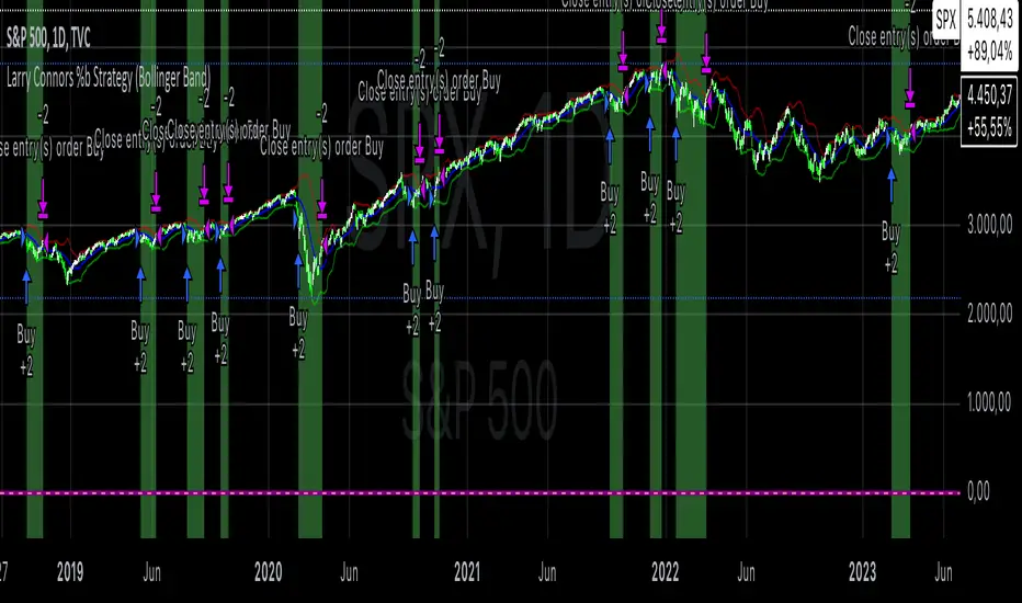
Larry Connors %b Strategy (Bollinger Band)Larry Connors’ %b Strategy is a mean-reversion trading approach that uses Bollinger Bands to identify buy and sell signals based on the %b indicator. This strategy was developed by Larry Connors, a renowned trader and author known for his systematic, data-driven trading methods, particularly those focusing on short-term mean reversion.
The %b indicator measures the position of the current price relative to the Bollinger Bands, which are volatility bands placed above and below a moving average. The strategy specifically targets times when prices are oversold within a long-term uptrend and aims to capture rebounds by buying at relatively low points and selling at relatively high points.
Strategy Rules
The basic rules of the %b Strategy are:
1. Trend Confirmation: The closing price must be above the 200-day moving average. This filter ensures that trades are made in alignment with a longer-term uptrend, thereby avoiding trades against the primary market trend.
2. Oversold Conditions: The %b indicator must be below 0.2 for three consecutive days. The %b value below 0.2 indicates that the price is near the lower Bollinger Band, suggesting an oversold condition.
3. Entry Signal: Enter a long position at the close when conditions 1 and 2 are met.
4. Exit Signal: Exit the position when the %b value closes above 0.8, signaling an overbought condition where the price is near the upper Bollinger Band.
How the Strategy Works
This strategy operates on the premise of mean reversion, which suggests that extreme price movements will revert to the mean over time. By entering positions when the %b value indicates an oversold condition (below 0.2) in a confirmed uptrend, the strategy attempts to capture short-term price rebounds. The exit rule (when %b is above 0.8) aims to lock in profits once the price reaches an overbought condition, often near the upper Bollinger Band.
Who Was Larry Connors?
Larry Connors is a well-known figure in the world of financial markets and trading. He co-authored several influential trading books, including “Short-Term Trading Strategies That Work” and “High Probability ETF Trading.” Connors is recognized for his quantitative approach, focusing on systematic, rules-based strategies that leverage historical data to validate trading edges.
His work primarily revolves around short-term trading strategies, often using technical indicators like RSI (Relative Strength Index), Bollinger Bands, and moving averages. Connors’ methodologies have been widely adopted by traders seeking structured approaches to exploit short-term inefficiencies in the market.
Risks of the Strategy
While the %b Strategy can be effective, particularly in mean-reverting markets, it is not without risks:
1. Mean Reversion Assumption: The strategy is based on the assumption that prices will revert to the mean. In trending or sharply falling markets, this reversion may not occur, leading to sustained losses.
2. False Signals in Choppy Markets: In volatile or sideways markets, the strategy may generate multiple false signals, resulting in whipsaw trades that can erode capital through frequent small losses.
3. No Stop Loss: The basic implementation of the strategy does not include a stop loss, which increases the risk of holding losing trades longer than intended, especially if the market continues to move against the position.
4. Performance During Market Crashes: During major market downturns, the strategy’s buy signals could be triggered frequently as prices decline, compounding losses without the presence of a risk management mechanism.
Scientific References and Theoretical Basis
The %b Strategy relies on the concept of mean reversion, which has been extensively studied in finance literature. Studies by Avellaneda and Lee (2010) and Bouchaud et al. (2018) have demonstrated that mean-reverting strategies can be profitable in specific market environments, particularly when combined with volatility filters like Bollinger Bands. However, the same studies caution that such strategies are highly sensitive to market conditions and often perform poorly during periods of prolonged trends.
Bollinger Bands themselves were popularized by John Bollinger and are widely used to assess price volatility and detect potential overbought and oversold conditions. The %b value is a critical part of this analysis, as it standardizes the position of price relative to the bands, making it easier to compare conditions across different securities and time frames.
Conclusion
Larry Connors’ %b Strategy is a well-known mean-reversion technique that leverages Bollinger Bands to identify buying opportunities in uptrending markets when prices are temporarily oversold. While the strategy can be effective under the right conditions, traders should be aware of its limitations and risks, particularly in trending or highly volatile markets. Incorporating risk management techniques, such as stop losses, could help mitigate some of these risks, making the strategy more robust against adverse market conditions.
Potential Divergence Checker#### Key Features
1. Potential Divergence Signals:
Potential divergences can signal a change in price movement before it occurs. This indicator identifies potential divergences instead of waiting for full confirmation, allowing it to detect signs of divergence earlier than traditional methods. This provides more flexible entry points and can act as a broader filter for potential setups.
2. Exposing Signals for External Use:
One of its advanced features is the ability to expose signals for use in other scripts. This allows users to integrate divergence signals and related entry/exit points into custom strategies or automated systems.
3. Custom Entry/Exit Timing Based on Years and Days:
The indicator provides entry and exit signals based on years and days, which could be useful for time-specific market behavior, long-term trades, and back testing.
#### Basic Usage
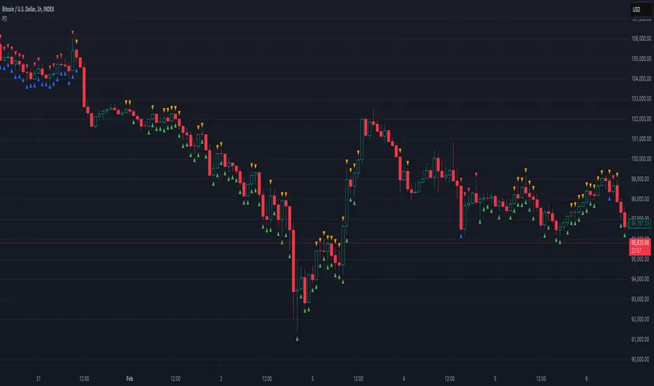
This indicator can check for all types of potential divergences: bullish, hidden bullish, bearish, hidden bearish. All you need to do is choose the type you want to check for under “DIVERGENCE TYPE” in the settings. On the chart, potential bullish divergences will show up as triangles below the price candles. one the chart potential bearish divergences will show up as upside down triangles above the price candles
#### Signals for Advanced Usage
You can use this indicator as a source in other indicators or strategies using the following information:
“ PD: Bull divergence signal ” will return “1” when a divergence is present and “0” when not present
“ PD: HBull divergence(hidden bull) signal ” will return “1” when a divergence is present and “0” when not present
“ PD: Bear divergence signal ” will return “1” when a divergence is present and “0” when not present
“ PD: HBear divergence(hidden bear) signal ” will return “1” when a divergence is present and “0” when not present
“ PD: enter ” signal will return a “1” when both the days and years criteria in the “entry filter settings” are met and “0” when not met.
“ PD: exit ” signal will return a “1” when the days criteria in the “exit filter settings” are met and “0” when not met.
#### Examples of Using Signals
1. If you are testing a long strategy for Bitcoin and do not want it to run during bear market years(e.g., the second year after a US presidential election), you can enable the “year and day filter for entry,” uncheck the following years in the settings: 2010, 2014, 2018, 2022, 2026, and reference the signal below in our strategy
signal: “ PD: enter ”
2. Let’s say you have a good long strategy, but want to make it a bit more profitable, you can tell the strategy not to run on days where there is potential bearish divergence and have it only run on more profitable days using these signals and the appropriate settings in the indicator
signal: “ PD: Bear divergence signal ” will return a ‘0’ with no bearish divergence present
signal: “ PD: enter ” will return a “1” if the entry falls on a specific, more profitable day chosen in the settings
#### Disclaimer
The "Potential Divergence Checker" indicator is a tool designed to identify potential market signals. It may have bugs and not do what it should do. It is not a guarantee of future trading performance, and users should exercise caution when making trading decisions based on its outputs. Always perform your own research and consider consulting with a financial advisor before making any investment decisions. Trading involves significant risk, and past performance is not indicative of future results.
Fractional Differentiation█ Description
This Pine Script indicator implements fractional differentiation, a mathematical operation that extends the concept of differentiation to non-integer orders. Fractional differentiation is particularly significant in financial analysis, as it enables analysts to uncover underlying patterns in price series that are not evident with traditional integer-order differentiation. The motivation behind fractional differencing lies in its ability to balance the trade-off between retaining data/feature memory and ensuring stationarity.
█ Significance
Fractional differentiation offers a nuanced view of market data, allowing for the adjustment of the differentiation order to balance between signal clarity and noise reduction. This is especially useful in financial markets, where the choice of differentiation order can highlight long-term trends or short-term price movements without completely smoothing out the valuable market noise.
█ Approximations Used
The implementation relies on the Gamma function for the computation of coefficients in the fractional differentiation formula. Given the complexity of the Gamma function, this script uses an approximation method based on the Lanczos approximation for the logarithm of the Gamma function, as detailed in "An Analysis Of The Lanczos Gamma Approximation" by Glendon Ralph Pugh (2004). This approximation strikes a balance between computational efficiency and accuracy, making it suitable for real-time market analysis in Pine Script.
█ Limitations
While this script opens new avenues for market analysis, it comes with inherent limitations:
- The approximation of the Gamma function, although accurate, is not exact. The precision of the fractional differentiation result may vary slightly, especially for higher-order differentiations.
- The script's performance is subject to Pine Script's execution environment, with a default loop limit set to 100 iterations for practicality. Users might need to adjust this limit based on their specific use case, balancing between computational load and the desired depth of historical data analysis.
█ Credits
This script makes use of the `MathSpecialFunctionsGamma` library, authored by Ricardo Santos . This library provides essential mathematical functions, including an approximation of the Gamma function, which is crucial for the fractional differentiation calculation.
I also extend my sincere gratitude to
Dr. Marcos López de Prado for his seminal work, Advances in Financial Machine Learning (2018). Dr. López de Prado's insights have significantly influenced our approach to developing sophisticated analytical tools.
Dr. Ernie Chan for his freely and generously sharing valuable insights via discourse on quantitative trading strategies through his talks and publications.
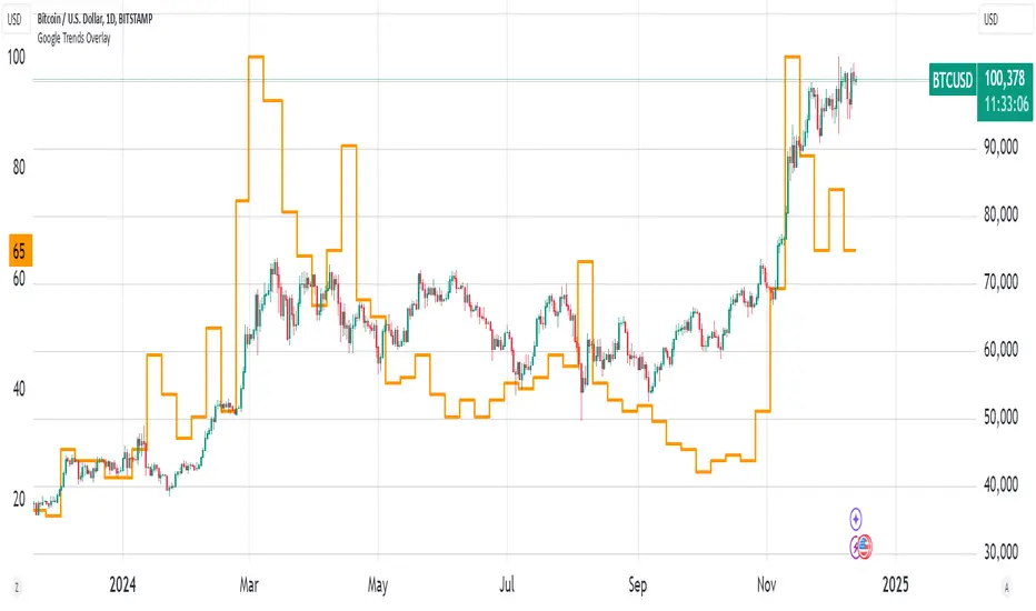
Bitcoin Google Trends OverlayThis indicator overlays Bitcoin Google trends data starting from 16/12/2018 until 10/12/2023. To have more recent data, you will need to update the data points manually.
If it is not showing properly, you need to plot the indicator to a new scale. Try also to use a logarithmic scale to better correlate the Bitcoin Google Trends data.
Interpretation:
Google Trends data and the Bitcoin price are very correlated. Google Trends data is a good indicator of market sentiment, but it usually lags.
EphemerisLibrary "Ephemeris"
TODO: add library description here
mercuryElements()
mercuryRates()
venusElements()
venusRates()
earthElements()
earthRates()
marsElements()
marsRates()
jupiterElements()
jupiterRates()
saturnElements()
saturnRates()
uranusElements()
uranusRates()
neptuneElements()
neptuneRates()
rev360(x)
Normalize degrees to within [0, 360)
Parameters:
x (float) : degrees to be normalized
Returns: Normalized degrees
scaleAngle(longitude, magnitude, harmonic)
Scale angle in degrees
Parameters:
longitude (float)
magnitude (float)
harmonic (int)
Returns: Scaled angle in degrees
julianCenturyInJulianDays()
Constant Julian days per century
Returns: 36525
julianEpochJ2000()
Julian date on J2000 epoch start (2000-01-01)
Returns: 2451545.0
meanObliquityForJ2000()
Mean obliquity of the ecliptic on J2000 epoch start (2000-01-01)
Returns: 23.43928
getJulianDate(Year, Month, Day, Hour, Minute)
Convert calendar date to Julian date
Parameters:
Year (int) : calendar year as integer (e.g. 2018)
Month (int) : calendar month (January = 1, December = 12)
Day (int) : calendar day of month (e.g. January valid days are 1-31)
Hour (int) : valid values 0-23
Minute (int) : valid values 0-60
julianCenturies(date, epoch_start)
Centuries since Julian Epoch 2000-01-01
Parameters:
date (float) : Julian date to conver to Julian centuries
epoch_start (float) : Julian date of epoch start (e.g. J2000 epoch = 2451545)
Returns: Julian date converted to Julian centuries
julianCenturiesSinceEpochJ2000(julianDate)
Calculate Julian centuries since epoch J2000 (2000-01-01)
Parameters:
julianDate (float) : Julian Date in days
Returns: Julian centuries since epoch J2000 (2000-01-01)
atan2(y, x)
Specialized arctan function
Parameters:
y (float) : radians
x (float) : radians
Returns: special arctan of y/x
eccAnom(ec, m_param, dp)
Compute eccentricity of the anomaly
Parameters:
ec (float) : Eccentricity of Orbit
m_param (float) : Mean Anomaly ?
dp (int) : Decimal places to round to
Returns: Eccentricity of the Anomaly
planetEphemerisCalc(TGen, planetElementId, planetRatesId)
Compute planetary ephemeris (longtude relative to Earth or Sun) on a Julian date
Parameters:
TGen (float) : Julian Date
planetElementId (float ) : All planet orbital elements in an array. This index references a specific planet's elements.
planetRatesId (float ) : All planet orbital rates in an array. This index references a specific planet's rates.
Returns: X,Y,Z ecliptic rectangular coordinates and R radius from reference body.
calculateRightAscensionAndDeclination(earthX, earthY, earthZ, planetX, planetY, planetZ)
Calculate right ascension and declination for a planet relative to Earth
Parameters:
earthX (float) : Earth X ecliptic rectangular coordinate relative to Sun
earthY (float) : Earth Y ecliptic rectangular coordinate relative to Sun
earthZ (float) : Earth Z ecliptic rectangular coordinate relative to Sun
planetX (float) : Planet X ecliptic rectangular coordinate relative to Sun
planetY (float) : Planet Y ecliptic rectangular coordinate relative to Sun
planetZ (float) : Planet Z ecliptic rectangular coordinate relative to Sun
Returns: Planet geocentric orbital radius, geocentric right ascension, and geocentric declination
mercuryHelio(T)
Compute Mercury heliocentric longitude on date
Parameters:
T (float)
Returns: Mercury heliocentric longitude on date
venusHelio(T)
Compute Venus heliocentric longitude on date
Parameters:
T (float)
Returns: Venus heliocentric longitude on date
earthHelio(T)
Compute Earth heliocentric longitude on date
Parameters:
T (float)
Returns: Earth heliocentric longitude on date
marsHelio(T)
Compute Mars heliocentric longitude on date
Parameters:
T (float)
Returns: Mars heliocentric longitude on date
jupiterHelio(T)
Compute Jupiter heliocentric longitude on date
Parameters:
T (float)
Returns: Jupiter heliocentric longitude on date
saturnHelio(T)
Compute Saturn heliocentric longitude on date
Parameters:
T (float)
Returns: Saturn heliocentric longitude on date
neptuneHelio(T)
Compute Neptune heliocentric longitude on date
Parameters:
T (float)
Returns: Neptune heliocentric longitude on date
uranusHelio(T)
Compute Uranus heliocentric longitude on date
Parameters:
T (float)
Returns: Uranus heliocentric longitude on date
sunGeo(T)
Parameters:
T (float)
mercuryGeo(T)
Parameters:
T (float)
venusGeo(T)
Parameters:
T (float)
marsGeo(T)
Parameters:
T (float)
jupiterGeo(T)
Parameters:
T (float)
saturnGeo(T)
Parameters:
T (float)
neptuneGeo(T)
Parameters:
T (float)
uranusGeo(T)
Parameters:
T (float)
moonGeo(T_JD)
Parameters:
T_JD (float)
mercuryOrbitalPeriod()
Mercury orbital period in Earth days
Returns: 87.9691
venusOrbitalPeriod()
Venus orbital period in Earth days
Returns: 224.701
earthOrbitalPeriod()
Earth orbital period in Earth days
Returns: 365.256363004
marsOrbitalPeriod()
Mars orbital period in Earth days
Returns: 686.980
jupiterOrbitalPeriod()
Jupiter orbital period in Earth days
Returns: 4332.59
saturnOrbitalPeriod()
Saturn orbital period in Earth days
Returns: 10759.22
uranusOrbitalPeriod()
Uranus orbital period in Earth days
Returns: 30688.5
neptuneOrbitalPeriod()
Neptune orbital period in Earth days
Returns: 60195.0
jupiterSaturnCompositePeriod()
jupiterNeptuneCompositePeriod()
jupiterUranusCompositePeriod()
saturnNeptuneCompositePeriod()
saturnUranusCompositePeriod()
planetSineWave(julianDateInCenturies, planetOrbitalPeriod, planetHelio)
Convert heliocentric longitude of planet into a sine wave
Parameters:
julianDateInCenturies (float)
planetOrbitalPeriod (float) : Orbital period of planet in Earth days
planetHelio (float) : Heliocentric longitude of planet in degrees
Returns: Sine of heliocentric longitude on a Julian date

Yesterday's High v.17.07Yesterday’s High Breakout it is a trading system based on the analysis of yesterday's highs, it works in trend-following mode therefore it opens a long position at the breakout of yesterday's highs even if they occur several times in one day.
There are several methods for exiting a trade, each with its own unique strategy. The first method involves setting Take-Profit and Stop-Loss percentages, while the second utilizes a trailing-stop with a specified offset value. The third method calls for a conditional exit when the candle closes below a reference EMA.
Additionally, operational filters can be applied based on the volatility of the currency pair, such as calculating the percentage change from the opening or incorporating a gap to the previous day's high levels. These filters help to anticipate or delay entry into the market, mitigating the risk of false breakouts.
In the specific case of INJ, a 12% Take-Profit and a 1.5% Stop-Loss were set, with an activated trailing-stop percentage, TRL 1 and OFF 0.5.
To postpone entry and avoid false breakouts, a 1% gap was added to the price of yesterday's highs.
Name: Yesterday's High Breakout - Trend Follower Strategy
Author: @tumiza999
Category: Trend Follower, Breakout of Yesterday's High.
Operating mode: Spot or Futures (only long).
Trade duration: Intraday.
Timeframe: 30M, 1H, 2H, 4H
Market: Crypto
Suggested usage: Short-term trading, when the market is in trend and it is showing high volatility.
Entry: When there is a breakout of Yesterday's High.
Exit: Profit target or Trailing stop, Stop loss or Crossunder EMA.
Configuration:
- Gap to anticipate or postpone the entry before or after the identified level
- Rate of Change for Entry Condition
- Take Profit, Stop Loss and Trailing Stop
- EMA length
Backtesting:
⁃ Exchange: BINANCE
⁃ Pair: INJUSDT
⁃ Timeframe: 4H
- Treshold: 1
- Gap%: 1
- SL: 1.5
- TP:12
- TRL: 1
- OFF-TRL: 0.5
⁃ Fee: 0.075%
⁃ Slippage: 1
- Initial Capital: 10000 USDT
- Position sizing: 10% of Equity
- Start : 2018-07-26 (Out Of Sample from 2022-12-23)
- Bar magnifier: on
Credits: LucF for Pine Coders (f_security function to avoid repainting using security)
Disclaimer: Risk Management is crucial, so adjust stop loss to your comfort level. A tight stop loss can help minimise potential losses. Use at your own risk.
How you or we can improve? Source code is open so share your ideas!
Leave a comment and smash the boost button!
Thanks for your attention, happy to support the TradingView community.

MA Correlation CoefficientThis script helps you visualize the correlation between the price of an asset and 4 moving averages of your choice. This indicator can help you identify trendy markets as well as trend-shifts.
Disclaimer
Bear in mind that there is always some lag when using Moving-Averages, hence the purpose of this indicator is as a trend identification tool rather than an entry-exit strategy.
Working Principle
The basic idea behind this indicator is the following:
In a trendy market you will find high correlation between price and all kinds of Moving-Averages. This works both ways, no matter bull or bear trend.
In sideways markets you might find a mix of correlations accross timeframes (2018) or high correlation with Low-Timeframe averages and low correlation with High-Timeframe averages (2021/2022).
Trend shifts might be characterised by a 'staircase' type of correlation (yellow), where the asset regains correlation with higher timeframe averages
Indicator Options
1. Source : data used for indicator calculation
1. Correlation Window : size of moving window for correlation calculation
2. Average Type :
Simple-Moving-Average (SMA)
Exponential-Moving-Average (EMA)
Hull-Moving-Average (HMA)
Volume-Weighted-Moving-Average (VWMA)
3. Lookback : number of past candles to calculate average
4. Gradient : modify gradient colors. colors relate to correlation values.
Plot Explanation
The indicator plots, using colors, the correlation of the asset with 4 averages. For every candle, 4 correlation values are generated, corresponding to 4 colors. These 4 colors are stacked one on top of the other generating the patterns explained above. These patterns may help you identify what kind of market you're in.

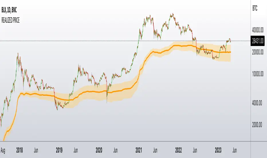
Realized PriceBitcoin Realized Price is a metric that determines the value of all bitcoins in circulation by dividing the total purchase price by the number of bitcoins. This provides traders with the average cost basis for all bitcoins in circulation, which is also known as Realized Price.
Unlike the current Market Price that reflects the current value of CRYPTOCAP:BTC , Realized Price shows the average purchase price of all bitcoins in circulation. It is essential to note that Realized Price values each UTXO based on the value when it last moved from one wallet to another, assuming that the movement represents the purchase of the bitcoins.
The significance of Bitcoin Realized Price lies in its ability to provide traders with an overall economic perspective of the Bitcoin market. When the CRYPTOCAP:BTC Market Price exceeds the Realized Price, the market participants are making a profit on average. Conversely, when the CRYPTOCAP:BTC Market Price is lower than the Realized Price, traders are incurring paper losses on average.
It's worth noting that Realized Price is a modification of Realized Cap, created in 2018 by Antoine Le Calvez.
In addition to BTC I have added LTC and ETH
NB!
Script is history data depended - use on charts with most history data
BTC -> BNC:BLX
ETH -> BITSTAMP:ETHUSD
LTC -> BITFINEX:LTCUSD
it plots realized price and its deviation - when price break out from these bands it explodes hard - near the realized price is good to accumulate the coin - it is fair price
Examples
BTC
ETH
LTC
Yesterday’s High Breakout - Trend Following StrategyYesterday’s High Breakout it is a trading system based on the analysis of yesterday's highs, it works in trend-following mode therefore it opens a long position at the breakout of yesterday's highs even if they occur several times in one day.
There are several methods for exiting a trade, each with its own unique strategy. The first method involves setting Take-Profit and Stop-Loss percentages, while the second utilizes a trailing-stop with a specified offset value. The third method calls for a conditional exit when the candle closes below a reference EMA.
Additionally, operational filters can be applied based on the volatility of the currency pair, such as calculating the percentage change from the opening or incorporating a gap to the previous day's high levels. These filters help to anticipate or delay entry into the market, mitigating the risk of false breakouts.
In the specific case of NULS, a 9% Take-Profit and a 3% Stop-Loss were set, with an activated trailing-stop percentage. To postpone entry and avoid false breakouts, a 1% gap was added to the price of yesterday's highs.
Name : Yesterday's High Breakout - Trend Follower Strategy
Author : @tumiza999
Category : Trend Follower, Breakout of Yesterday's High.
Operating mode : Spot or Futures (only long).
Trade duration : Intraday.
Timeframe : 30M, 1H, 2H, 4H
Market : Crypto
Suggested usage : Short-term trading, when the market is in trend and it is showing high volatility.
Entry : When there is a breakout of Yesterday's High.
Exit : Profit target or Trailing stop, Stop loss or Crossunder EMA.
Configuration :
- Gap to anticipate or postpone the entry before or after the identified level
- Rate of Change for Entry Condition
- Take Profit, Stop Loss and Trailing Stop
- EMA length
Backtesting :
⁃ Exchange: BINANCE
⁃ Pair: NULSUSDT
⁃ Timeframe: 2H
⁃ Fee: 0.075%
⁃ Slippage: 1
- Initial Capital: 10000 USDT
- Position sizing: 10% of Equity
- Start : 2018-07-26 (Out Of Sample from 2022-12-23)
- Bar magnifier: on
Credits : LucF for Pine Coders (f_security function to avoid repainting using security)
Disclaimer : Risk Management is crucial, so adjust stop loss to your comfort level. A tight stop loss can help minimise potential losses. Use at your own risk.
How you or we can improve? Source code is open so share your ideas!
Leave a comment and smash the boost button!
Thanks for your attention, happy to support the TradingView community.

Price Distance RatioThis study plots the ratio between current price and the price N days ago.
With N input that is configurable, users can find optimal long/short entries when price is in an established trend and price has diverge far from a given local peak or all time high.
With many years of stock trading the analysis indicates a connection between the distance of price and subsequent returns.
Portfolios of stocks with lower price to local highes ratios generally underperformed portfolios of stocks with higher prices to peaks reached similar N days ago.
The highest returns to previous peak are recorded when buying at the biggest dip.
For example, the purchase at 20% drawdown could generate 25% when price returns to the peak. The purchase at 50% drawdown could generate bigger, i.e. 100% return, when price returns to the peak. And the purchase at 90% drawdown could generate much bigger, i.e. 900% return, in a case the price returns to the peak.
However, buying very far below local peaks on almost all holding periods produces lower CAGR returns because of "timing adjustment". In simple words, typically the drawdown takes less time vs. further recovery.
For example:
👉 The largest BTC drawdown in 2013-2015 took 410 days (Peak-to-Valley) . And the recovery of BTC to new highs took 771 days (Valley-to-Peak) after that.
👉 The 3rd longest drawdown in BTC took 363 days (observed from December 17, 2017 to December 15, 2018). And further recovery in BTC to its new high took almost two years - 716 days .
👉The 4th longest drawdown in BTC took 162 days (observed from June 08, 2011 to November 17, 2011). And further recovery in BTC to its new high took more than a year - 469 days .
The concept of this study could recognizes at least 4 different modes of action.
👉 In a clearly established upward trend traders should be buying (following the trend) when Ratio is above 100% and reducing the size when Ratio turns below 100%.
👉 Conversely, in a clearly established downward trend traders should be shorted when Ratio is below 100% and covering when the Ratio turns back to 100%.
👉 In a sideways movement traders are advised to wait carefully if the Ratio near 100% for a long time, and take a position the trend is clear.
👉 Chartists can analyze the dynamic of the indicator - both in terms of trends and overall level. For example as it shown at the chart.
The understading of the study and rules of "timing adjustments" could genarate the awesome opportunities for stock options traders also, with strategies of selling uncovered call options and vertical call spreads.
// Many thanks to @HPotter and @Wheeelman wizards for their continious support and assistance.

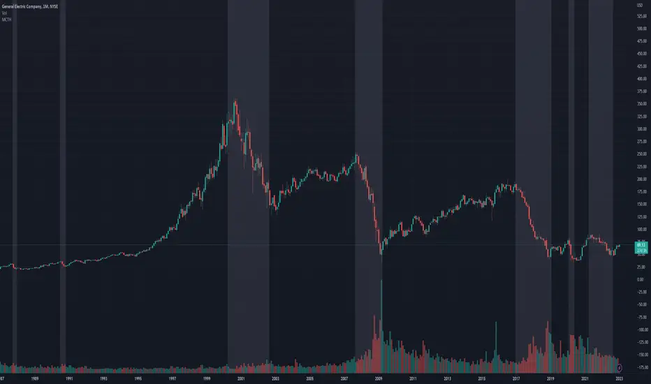
Market Crashes/Chart Timeframes HighlightThis extremely helpful indicator allows you to highlight 7 custom date-based timeframes on your charts.
The default dates selected are what I consider to be the most significant 7 most recent market declines, including and since the 87 flash crash.
Note: The default dates are approximate but good enough to highlight the key timeframes of these pullbacks/crashes/corrections.
It's simple to use and does exactly what it should.
I created this indicator to make it easier when looking at the overall story of a chart. I found it helpful to highlight these areas to see how a market or equity has responded during these significant market pullbacks.
The highlight alone I’ve found helpful, and it becomes more powerful if you combine it with your own trusted trade system.
Also, to get the most out of using the default dates it’s important to understand the narrative behind each pullback/crash. Here’s the list of what I consider significant pullbacks:
Black Monday - Oct 87
1990s Recession - Jul 90 to Mar 91
Dot Com Bubble - 2000 to 2002 or so
Real Estate 2008 Crisis - I choose 2007-2009 to cover full insider knowledge and aftermath
2016 - 2018 - This isn't seen as a pullback, but I have it as significant because in many markets and equities, this was an almost equal percentage pullback as 2008. See Notes below
2020 Crash - Covid-19 and related shenanigans pullback
April 2021 to August 2022 - I believe we are in a current SHORT cycle so I've highlighted April 2021 as the start of what might be the start of a major decline testing Dot Com or lower levels.
A few notes on the above.
You'll find on most of the pullbacks listed above most equities and related markets behave similarly or have similar patterns.
The 2016-18 pullback is the most difficult to track. For instance, GE in this timeframe had a -80% decline, whereas BA depending on how you want to measure it had a 50-110% gain.
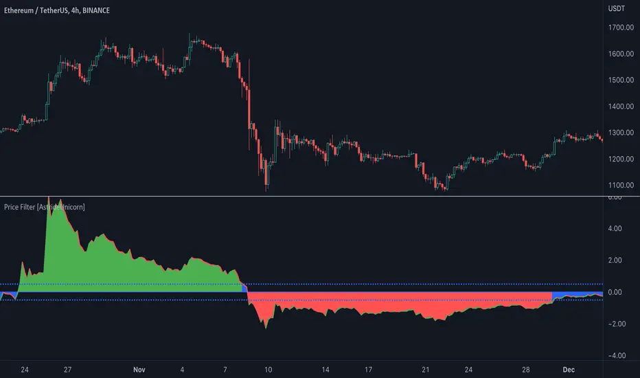
Price Filter [AstrideUnicorn]The indicator calculates a fast price filter based on the closing price of the underlying asset. Overall, it is intended to provide a fast, reliable way to detect trend direction and confirm trend strength, using statistical measures of price movements.
The algorithm was adapted from Marcus Schmidberger's (2018) article "High Frequency Trading with the MSCI World ETF". It demeans the price time series using the long-term average and then normalizes it with the long-term standard deviation. The resulting time series is then compared to specified thresholds to determine the trend direction.
HOW TO USE
The indicator surface is colored green if the price is trending upwards and red if the price is trending downwards. If the indicator outline is the opposite color of the indicator surface, it indicates that the price is moving against the trend and the current trend may be losing strength.
If the 'Use threshold' setting is enabled, the indicator will be colored blue if its value is within the range defined by the upper and lower thresholds. This indicates that the price is trending sideways, or that the current trend is losing strength.
SETTNGS
Length - the length of the long-term average used to calculate the price filter. Recommended range 20 - 200. The sensitivity of the indicator increases as the value becomes smaller, allowing it to detect smaller price moves and swings earlier.
Threshold - the threshold value used to detect trend direction.
Use threshold - a boolean (true/false) input that determines whether to use the threshold value for confirmation.
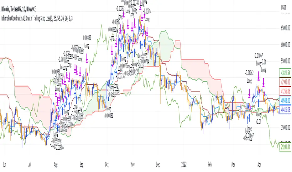
Ichimoku Cloud and ADX with Trailing Stop Loss (by Coinrule)The Ichimoku Cloud is a collection of technical indicators that show support and resistance levels, as well as momentum and trend direction. It does this by taking multiple averages and plotting them on a chart. It also uses these figures to compute a “cloud” that attempts to forecast where the price may find support or resistance in the future.
The Ichimoku Cloud was developed by Goichi Hosoda, a Japanese journalist, and published in the late 1960s. It provides more data points than the standard candlestick chart. While it seems complicated at first glance, those familiar with how to read the charts often find it easy to understand with well-defined trading signals.
The Ichimoku Cloud is composed of five lines or calculations, two of which comprise a cloud where the difference between the two lines is shaded in.
The lines include a nine-period average, a 26-period average, an average of those two averages, a 52-period average, and a lagging closing price line.
The cloud is a key part of the indicator. When the price is below the cloud, the trend is down. When the price is above the cloud, the trend is up.
The above trend signals are strengthened if the cloud is moving in the same direction as the price. For example, during an uptrend, the top of the cloud is moving up, or during a downtrend, the bottom of the cloud is moving down.
DMI is simple to interpret. When +DI > - DI, it means the price is trending up. On the other hand, when -DI > +DI , the trend is weak or moving on the downside. The ADX does not give an indication about the direction but about the strength of the trend.
Typically values of ADX above 25 mean that the trend is steeply moving up or down, based on the -DI and +D positioning. This script aims to capture swings in the DMI, and thus, in the trend of the asset, using a contrarian approach.
Trading on high values of ADX, the strategy tries to spot extremely oversold and overbought conditions. Values of ADX above 45 may suggest that the trend has overextended and is may be about to reverse.
This strategy combines the Ichimoku Cloud with the ADX indicator to better enter trades.
Long orders are placed when these basic signals are triggered.
Long Position:
Tenkan-Sen is above the Kijun-Sen
Chikou-Span is above the close of 26 bars ago
Close is above the Kumo Cloud
MACD line crosses over the signal line
-DI is greater than +DI
ADX is greater than 45
Close Position:
3% increase trailing
3% decrease trailing
The script is backtested from 1 January 2018 and provides good returns.
The strategy assumes each order is using 30% of the available coins to make the results more realistic and to simulate you only ran this strategy on 30% of your holdings. A trading fee of 0.1% is also taken into account and is aligned to the base fee applied on Binance.
This script also works well on MATIC (1d timeframe), ETH (1d timeframe), and SOL (1d timeframe).
Event Locator BasicUsable under any conditions and in all markets, the 'event locator' provides a foundational layer for any count-based trading strategy or system. This specific installment color codes events - all down events are green, up events are blue, double-marked events are red, and smooth events are gray. It also wraps the price sequence in a 3-d line landscape plot - providing a visual using lines that are event sensitive. Though events are sometimes referred to as 'fractals,' this is not a fractal tool. These marks are based on 3 candles, not 5 as is common with the Bill Williams fractal scripts. Every countable event on the chart will be marked using this tool. Really, Elliott Wave should have told you about this... (because you can't legitimately count w/o it)
//This indicator was originally a mod of the 'Williams Fractals' indicator - modified by Erek A.D., Nov. 2017
//It was rewritten from the ground up by 'Brobear' in Sept./Oct. 2018
//This code marks 'rough' AND 'smooth' EVENTS in price flow
//EVENTS are naturally created in markets when SEPARATION occurs at candle tips
//SEPARATION happens when a high is flanked by lower highs or a low is flanked by higher lows
//EVENT LOCATORS like this provide an objective foundation for counting price movement
