Aetherium Institutional Market Resonance EngineAetherium Institutional Market Resonance Engine (AIMRE)
A Three-Pillar Framework for Decoding Institutional Activity
🎓 THEORETICAL FOUNDATION
The Aetherium Institutional Market Resonance Engine (AIMRE) is a multi-faceted analysis system designed to move beyond conventional indicators and decode the market's underlying structure as dictated by institutional capital flow. Its philosophy is built on a singular premise: significant market moves are preceded by a convergence of context , location , and timing . Aetherium quantifies these three dimensions through a revolutionary three-pillar architecture.
This system is not a simple combination of indicators; it is an integrated engine where each pillar's analysis feeds into a central logic core. A signal is only generated when all three pillars achieve a state of resonance, indicating a high-probability alignment between market organization, key liquidity levels, and cyclical momentum.
⚡ THE THREE-PILLAR ARCHITECTURE
1. 🌌 PILLAR I: THE COHERENCE ENGINE (THE 'CONTEXT')
Purpose: To measure the degree of organization within the market. This pillar answers the question: " Is the market acting with a unified purpose, or is it chaotic and random? "
Conceptual Framework: Institutional campaigns (accumulation or distribution) create a non-random, organized market environment. Retail-driven or directionless markets are characterized by "noise" and chaos. The Coherence Engine acts as a filter to ensure we only engage when institutional players are actively steering the market.
Formulaic Concept:
Coherence = f(Dominance, Synchronization)
Dominance Factor: Calculates the absolute difference between smoothed buying pressure (volume-weighted bullish candles) and smoothed selling pressure (volume-weighted bearish candles), normalized by total pressure. A high value signifies a clear winner between buyers and sellers.
Synchronization Factor: Measures the correlation between the streams of buying and selling pressure over the analysis window. A high positive correlation indicates synchronized, directional activity, while a negative correlation suggests choppy, conflicting action.
The final Coherence score (0-100) represents the percentage of market organization. A high score is a prerequisite for any signal, filtering out unpredictable market conditions.
2. 💎 PILLAR II: HARMONIC LIQUIDITY MATRIX (THE 'LOCATION')
Purpose: To identify and map high-impact institutional footprints. This pillar answers the question: " Where have institutions previously committed significant capital? "
Conceptual Framework: Large institutional orders leave indelible marks on the market in the form of anomalous volume spikes at specific price levels. These are not random occurrences but are areas of intense historical interest. The Harmonic Liquidity Matrix finds these footprints and consolidates them into actionable support and resistance zones called "Harmonic Nodes."
Algorithmic Process:
Footprint Identification: The engine scans the historical lookback period for candles where volume > average_volume * Institutional_Volume_Filter. This identifies statistically significant volume events.
Node Creation: A raw node is created at the mean price of the identified candle.
Dynamic Clustering: The engine uses an ATR-based proximity algorithm. If a new footprint is identified within Node_Clustering_Distance (ATR) of an existing Harmonic Node, it is merged. The node's price is volume-weighted, and its magnitude is increased. This prevents chart clutter and consolidates nearby institutional orders into a single, more significant level.
Node Decay: Nodes that are older than the Institutional_Liquidity_Scanback period are automatically removed from the chart, ensuring the analysis remains relevant to recent market dynamics.
3. 🌊 PILLAR III: CYCLICAL RESONANCE MATRIX (THE 'TIMING')
Purpose: To identify the market's dominant rhythm and its current phase. This pillar answers the question: " Is the market's immediate energy flowing up or down? "
Conceptual Framework: Markets move in waves and cycles of varying lengths. Trading in harmony with the current cyclical phase dramatically increases the probability of success. Aetherium employs a simplified wavelet analysis concept to decompose price action into short, medium, and long-term cycles.
Algorithmic Process:
Cycle Decomposition: The engine calculates three oscillators based on the difference between pairs of Exponential Moving Averages (e.g., EMA8-EMA13 for short cycle, EMA21-EMA34 for medium cycle).
Energy Measurement: The 'energy' of each cycle is determined by its recent volatility (standard deviation). The cycle with the highest energy is designated as the "Dominant Cycle."
Phase Analysis: The engine determines if the dominant cycles are in a bullish phase (rising from a trough) or a bearish phase (falling from a peak).
Cycle Sync: The highest conviction timing signals occur when multiple cycles (e.g., short and medium) are synchronized in the same direction, indicating broad-based momentum.
🔧 COMPREHENSIVE INPUT SYSTEM
Pillar I: Market Coherence Engine
Coherence Analysis Window (10-50, Default: 21): The lookback period for the Coherence Engine.
Lower Values (10-15): Highly responsive to rapid shifts in market control. Ideal for scalping but can be sensitive to noise.
Balanced (20-30): Excellent for day trading, capturing the ebb and flow of institutional sessions.
Higher Values (35-50): Smoother, more stable reading. Best for swing trading and identifying long-term institutional campaigns.
Coherence Activation Level (50-90%, Default: 70%): The minimum market organization required to enable signal generation.
Strict (80-90%): Only allows signals in extremely clear, powerful trends. Fewer, but potentially higher quality signals.
Standard (65-75%): A robust filter that effectively removes choppy conditions while capturing most valid institutional moves.
Lenient (50-60%): Allows signals in less-organized markets. Can be useful in ranging markets but may increase false signals.
Pillar II: Harmonic Liquidity Matrix
Institutional Liquidity Scanback (100-400, Default: 200): How far back the engine looks for institutional footprints.
Short (100-150): Focuses on recent institutional activity, providing highly relevant, immediate levels.
Long (300-400): Identifies major, long-term structural levels. These nodes are often extremely powerful but may be less frequent.
Institutional Volume Filter (1.3-3.0, Default: 1.8): The multiplier for detecting a volume spike.
High (2.5-3.0): Only registers climactic, undeniable institutional volume. Fewer, but more significant nodes.
Low (1.3-1.7): More sensitive, identifying smaller but still relevant institutional interest.
Node Clustering Distance (0.2-0.8 ATR, Default: 0.4): The ATR-based distance for merging nearby nodes.
High (0.6-0.8): Creates wider, more consolidated zones of liquidity.
Low (0.2-0.3): Creates more numerous, precise, and distinct levels.
Pillar III: Cyclical Resonance Matrix
Cycle Resonance Analysis (30-100, Default: 50): The lookback for determining cycle energy and dominance.
Short (30-40): Tunes the engine to faster, shorter-term market rhythms. Best for scalping.
Long (70-100): Aligns the timing component with the larger primary trend. Best for swing trading.
Institutional Signal Architecture
Signal Quality Mode (Professional, Elite, Supreme): Controls the strictness of the three-pillar confluence.
Professional: Loosest setting. May generate signals if two of the three pillars are in strong alignment. Increases signal frequency.
Elite: Balanced setting. Requires a clear, unambiguous resonance of all three pillars. The recommended default.
Supreme: Most stringent. Requires perfect alignment of all three pillars, with each pillar exhibiting exceptionally strong readings (e.g., coherence > 85%). The highest conviction signals.
Signal Spacing Control (5-25, Default: 10): The minimum bars between signals to prevent clutter and redundant alerts.
🎨 ADVANCED VISUAL SYSTEM
The visual architecture of Aetherium is designed not merely for aesthetics, but to provide an intuitive, at-a-glance understanding of the complex data being processed.
Harmonic Liquidity Nodes: The core visual element. Displayed as multi-layered, semi-transparent horizontal boxes.
Magnitude Visualization: The height and opacity of a node's "glow" are proportional to its volume magnitude. More significant nodes appear brighter and larger, instantly drawing the eye to key levels.
Color Coding: Standard nodes are blue/purple, while exceptionally high-magnitude nodes are highlighted in an accent color to denote critical importance.
🌌 Quantum Resonance Field: A dynamic background gradient that visualizes the overall market environment.
Color: Shifts from cool blues/purples (low coherence) to energetic greens/cyans (high coherence and organization), providing instant context.
Intensity: The brightness and opacity of the field are influenced by total market energy (a composite of coherence, momentum, and volume), making powerful market states visually apparent.
💎 Crystalline Lattice Matrix: A geometric web of lines projected from a central moving average.
Mathematical Basis: Levels are projected using multiples of the Golden Ratio (Phi ≈ 1.618) and the ATR. This visualizes the natural harmonic and fractal structure of the market. It is not arbitrary but is based on mathematical principles of market geometry.
🧠 Synaptic Flow Network: A dynamic particle system visualizing the engine's "thought process."
Node Density & Activation: The number of particles and their brightness/color are tied directly to the Market Coherence score. In high-coherence states, the network becomes a dense, bright, and organized web. In chaotic states, it becomes sparse and dim.
⚡ Institutional Energy Waves: Flowing sine waves that visualize market volatility and rhythm.
Amplitude & Speed: The height and speed of the waves are directly influenced by the ATR and volume, providing a feel for market energy.
📊 INSTITUTIONAL CONTROL MATRIX (DASHBOARD)
The dashboard is the central command console, providing a real-time, quantitative summary of each pillar's status.
Header: Displays the script title and version.
Coherence Engine Section:
State: Displays a qualitative assessment of market organization: ◉ PHASE LOCK (High Coherence), ◎ ORGANIZING (Moderate Coherence), or ○ CHAOTIC (Low Coherence). Color-coded for immediate recognition.
Power: Shows the precise Coherence percentage and a directional arrow (↗ or ↘) indicating if organization is increasing or decreasing.
Liquidity Matrix Section:
Nodes: Displays the total number of active Harmonic Liquidity Nodes currently being tracked.
Target: Shows the price level of the nearest significant Harmonic Node to the current price, representing the most immediate institutional level of interest.
Cycle Matrix Section:
Cycle: Identifies the currently dominant market cycle (e.g., "MID ") based on cycle energy.
Sync: Indicates the alignment of the cyclical forces: ▲ BULLISH , ▼ BEARISH , or ◆ DIVERGENT . This is the core timing confirmation.
Signal Status Section:
A unified status bar that provides the final verdict of the engine. It will display "QUANTUM SCAN" during neutral periods, or announce the tier and direction of an active signal (e.g., "◉ TIER 1 BUY ◉" ), highlighted with the appropriate color.
🎯 SIGNAL GENERATION LOGIC
Aetherium's signal logic is built on the principle of strict, non-negotiable confluence.
Condition 1: Context (Coherence Filter): The Market Coherence must be above the Coherence Activation Level. No signals can be generated in a chaotic market.
Condition 2: Location (Liquidity Node Interaction): Price must be actively interacting with a significant Harmonic Liquidity Node.
For a Buy Signal: Price must be rejecting the Node from below (testing it as support).
For a Sell Signal: Price must be rejecting the Node from above (testing it as resistance).
Condition 3: Timing (Cycle Alignment): The Cyclical Resonance Matrix must confirm that the dominant cycles are synchronized with the intended trade direction.
Signal Tiering: The Signal Quality Mode input determines how strictly these three conditions must be met. 'Supreme' mode, for example, might require not only that the conditions are met, but that the Market Coherence is exceptionally high and the interaction with the Node is accompanied by a significant volume spike.
Signal Spacing: A final filter ensures that signals are spaced by a minimum number of bars, preventing over-alerting in a single move.
🚀 ADVANCED TRADING STRATEGIES
The Primary Confluence Strategy: The intended use of the system. Wait for a Tier 1 (Elite/Supreme) or Tier 2 (Professional/Elite) signal to appear on the chart. This represents the alignment of all three pillars. Enter after the signal bar closes, with a stop-loss placed logically on the other side of the Harmonic Node that triggered the signal.
The Coherence Context Strategy: Use the Coherence Engine as a standalone market filter. When Coherence is high (>70%), favor trend-following strategies. When Coherence is low (<50%), avoid new directional trades or favor range-bound strategies. A sharp drop in Coherence during a trend can be an early warning of a trend's exhaustion.
Node-to-Node Trading: In a high-coherence environment, use the Harmonic Liquidity Nodes as both entry points and profit targets. For example, after a BUY signal is generated at one Node, the next Node above it becomes a logical first profit target.
⚖️ RESPONSIBLE USAGE AND LIMITATIONS
Decision Support, Not a Crystal Ball: Aetherium is an advanced decision-support tool. It is designed to identify high-probability conditions based on a model of institutional behavior. It does not predict the future.
Risk Management is Paramount: No indicator can replace a sound risk management plan. Always use appropriate position sizing and stop-losses. The signals provided are probabilistic, not certainties.
Past Performance Disclaimer: The market models used in this script are based on historical data. While robust, there is no guarantee that these patterns will persist in the future. Market conditions can and do change.
Not a "Set and Forget" System: The indicator performs best when its user understands the concepts behind the three pillars. Use the dashboard and visual cues to build a comprehensive view of the market before acting on a signal.
Backtesting is Essential: Before applying this tool to live trading, it is crucial to backtest and forward-test it on your preferred instruments and timeframes to understand its unique behavior and characteristics.
🔮 CONCLUSION
The Aetherium Institutional Market Resonance Engine represents a paradigm shift from single-variable analysis to a holistic, multi-pillar framework. By quantifying the abstract concepts of market context, location, and timing into a unified, logical system, it provides traders with an unprecedented lens into the mechanics of institutional market operations.
It is not merely an indicator, but a complete analytical engine designed to foster a deeper understanding of market dynamics. By focusing on the core principles of institutional order flow, Aetherium empowers traders to filter out market noise, identify key structural levels, and time their entries in harmony with the market's underlying rhythm.
"In all chaos there is a cosmos, in all disorder a secret order." - Carl Jung
— Dskyz, Trade with insight. Trade with confluence. Trade with Aetherium.
Cerca negli script per "美国要强买强卖,要求中国购买指定商品,四年还必须买够15万亿?"

Options Strategy V1.3📈 Options Strategy V1.3 — EMA Crossover + RSI + ATR + Opening Range
Overview:
This strategy is designed for short-term directional trades on large-cap stocks or ETFs, especially when trading options. It combines classic trend-following signals with momentum confirmation, volatility-based risk management, and session timing filters to help identify high-probability entries with predefined stop-loss and profit targets.
🔍 Strategy Components:
EMA Crossover (Fast/Slow)
Entry signals are triggered by the crossover of a short EMA above or below a long EMA — a traditional trend-following method to detect shifts in momentum.
RSI Filter
RSI confirms the signal by avoiding entries in overbought/oversold zones unless certain momentum conditions are met.
Long entry requires RSI ≥ Long Threshold
Short entry requires RSI ≤ Short Threshold
ATR-Based SL & TP
Stop-loss is set dynamically as a multiple of ATR below (long) or above (short) the entry price.
Take-profit is placed as a ratio (TP/SL) of the stop distance, ensuring consistent reward/risk structure.
Opening Range Filter (Optional)
If enabled, the strategy only triggers trades after price breaks out of the 09:30–09:45 EST range, ensuring participation in directional moves.
Session Filters
No trades from 04:00 to 09:30 and from 16:00 to 20:00 EST, avoiding low-liquidity periods.
All open trades are closed at 15:55 EST, to avoid overnight risk or expiration issues for options.
⚙️ Built-in Presets:
You can choose one of the built-in ticker-specific presets for optimal conditions:
Ticker EMAs RSI (Long/Short) ATR SL×ATR TP/SL
SPY 8/28 56 / 26 14 1.4× 4.0×
TSLA 23/27 56 / 33 13 1.4× 3.6×
AAPL 6/13 61 / 26 23 1.4× 2.1×
MSFT 25/32 54 / 26 14 1.2× 2.2×
META 25/32 53 / 26 17 1.8× 2.3×
AMZN 28/32 55 / 25 16 1.8× 2.3×
You can also choose "Custom" to fully configure all parameters to your own market and strategy preferences.
📌 Best Use Case:
This strategy is especially suited for intraday options trading, where timing and risk control are critical. It works best on liquid tickers with strong trends or clear breakout behavior.

Open Range Breakout (ORB) with Alerts
🚀 ChartsAlgo – Open Range Breakout (ORB) with Alerts
The Open Range Breakout (ORB) Indicator by ChartsAlg is designed for intraday traders looking to capitalize on price movements after the market’s opening range. This tool is especially effective for futures (MNQ, MES) and high-volatility stocks or crypto where initial volatility sets the tone for the session.
This indicator identifies a user-defined opening range window, plots the high/low lines of that range, and visually alerts users when price breaks out above or below the range — with options to customize breakout repetitions, background fill, and alerts.
💡 What is an Open Range Breakout (ORB)?
The opening range represents the high and low established during the first few minutes of the trading session — usually 15 or 30 minutes. Many intraday strategies are based on the idea that breaking out of this initial range often signals strong momentum and trend continuation.
Traders often enter:
Long when price breaks above the range high.
Short when price breaks below the range low.
⚙️ How It Works
You define a session window (e.g., 09:30–09:45 EST).
The indicator tracks the high and low during this time.
Once the session ends, the high and low become your range breakout levels.
The indicator then:
Plots lines for visual clarity
Optionally fills background between the range
Triggers breakout signals if price crosses the levels
Provides alerts when breakouts occur
🛠️ Settings Breakdown
🔹 Session Settings
Range Session: Set your preferred window (e.g., 0930–0945). Can be premarket, first 30 mins, or any custom time.
Time zone: Use "America/New York" for EST (default) or change to "GMT+0" for international traders.
🔹 Breakout Settings
Bullish Breakout Signals: Number of allowed breakout alerts above the range.
Bearish Breakout Signals: Number of allowed breakout alerts below the range.
This prevents repeated alerts once breakout has been confirmed.
🔹 Display Settings
Show Background Fill: Fills area between high/low of the range for easier visual analysis.
Show Breakout Signals: Triangle markers plotted on the chart when breakouts happen.
Only Show Today’s Range: Keeps the chart clean by showing only the most current day’s range.
🔹 Color Settings
Range High/Low Line Colors: Choose any color for clarity.
Range Fill Color: Customize the highlight area for your chart style.
📊 Chart Features
Range High/Low Lines: Automatically plotted after range session ends.
Visual Fill Box: Optional background shading between the opening range.
Triangle Breakout Markers: Appear at the breakout candle.
Alerts: Can be used with TradingView’s alert system to notify you of breakouts in real-time.
🔔 Alerts
Two alert conditions are built in:
Bullish Breakout: Triggers when price breaks above the high of the range.
Bearish Breakout: Triggers when price breaks below the low of the range.
Example Alert Message:
📈 “Bullish Breakout above Open Range on AAPL!”
To activate:
Click “🔔 Alerts” on TradingView.
Set condition to this script.
Choose “ORB Breakout Up” or “ORB Breakout Down”.
Choose alert frequency and notification method.
⚠️ DISCLAIMER
ChartsAlgo tools are for informational and educational purposes only.
They are not financial advice or signals. Past performance does not guarantee future results. Use at your own risk and always implement solid risk management.
By using this indicator, you agree that you are solely responsible for any trades or decisions made based on the information provided.
Multi-Confluence Swing Hunter V1# Multi-Confluence Swing Hunter V1 - Complete Description
Overview
The Multi-Confluence Swing Hunter V1 is a sophisticated low timeframe scalping strategy specifically optimized for MSTR (MicroStrategy) trading. This strategy employs a comprehensive point-based scoring system that combines optimized technical indicators, price action analysis, and reversal pattern recognition to generate precise trading signals on lower timeframes.
Performance Highlight:
In backtesting on MSTR 5-minute charts, this strategy has demonstrated over 200% profit performance, showcasing its effectiveness in capturing rapid price movements and volatility patterns unique to MicroStrategy's trading behavior.
The strategy's parameters have been fine-tuned for MSTR's unique volatility characteristics, though they can be optimized for other high-volatility instruments as well.
## Key Innovation & Originality
This strategy introduces a unique **dual scoring system** approach:
- **Entry Scoring**: Identifies swing bottoms using 13+ different technical criteria
- **Exit Scoring**: Identifies swing tops using inverse criteria for optimal exit timing
Unlike traditional strategies that rely on simple indicator crossovers, this system quantifies market conditions through a weighted scoring mechanism, providing objective, data-driven entry and exit decisions.
## Technical Foundation
### Optimized Indicator Parameters
The strategy utilizes extensively backtested parameters specifically optimized for MSTR's volatility patterns:
**MACD Configuration (3,10,3)**:
- Fast EMA: 3 periods (vs standard 12)
- Slow EMA: 10 periods (vs standard 26)
- Signal Line: 3 periods (vs standard 9)
- **Rationale**: These faster parameters provide earlier signal detection while maintaining reliability, particularly effective for MSTR's rapid price movements and high-frequency volatility
**RSI Configuration (21-period)**:
- Length: 21 periods (vs standard 14)
- Oversold: 30 level
- Extreme Oversold: 25 level
- **Rationale**: The 21-period RSI reduces false signals while still capturing oversold conditions effectively in MSTR's volatile environment
**Parameter Adaptability**: While optimized for MSTR, these parameters can be adjusted for other high-volatility instruments. Faster-moving stocks may benefit from even shorter MACD periods, while less volatile assets might require longer periods for optimal performance.
### Scoring System Methodology
**Entry Score Components (Minimum 13 points required)**:
1. **RSI Signals** (max 5 points):
- RSI < 30: +2 points
- RSI < 25: +2 points
- RSI turning up: +1 point
2. **MACD Signals** (max 8 points):
- MACD below zero: +1 point
- MACD turning up: +2 points
- MACD histogram improving: +2 points
- MACD bullish divergence: +3 points
3. **Price Action** (max 4 points):
- Long lower wick (>50%): +2 points
- Small body (<30%): +1 point
- Bullish close: +1 point
4. **Pattern Recognition** (max 8 points):
- RSI bullish divergence: +4 points
- Quick recovery pattern: +2 points
- Reversal confirmation: +4 points
**Exit Score Components (Minimum 13 points required)**:
Uses inverse criteria to identify swing tops with similar weighting system.
## Risk Management Features
### Position Sizing & Risk Control
- **Single Position Strategy**: 100% equity allocation per trade
- **No Overlapping Positions**: Ensures focused risk management
- **Configurable Risk/Reward**: Default 5:1 ratio optimized for volatile assets
### Stop Loss & Take Profit Logic
- **Dynamic Stop Loss**: Based on recent swing lows with configurable buffer
- **Risk-Based Take Profit**: Calculated using risk/reward ratio
- **Clean Exit Logic**: Prevents conflicting signals
## Default Settings Optimization
### Key Parameters (Optimized for MSTR/Bitcoin-style volatility):
- **Minimum Entry Score**: 13 (ensures high-conviction entries)
- **Minimum Exit Score**: 13 (prevents premature exits)
- **Risk/Reward Ratio**: 5.0 (accounts for volatility)
- **Lower Wick Threshold**: 50% (identifies true hammer patterns)
- **Divergence Lookback**: 8 bars (optimal for swing timeframes)
### Why These Defaults Work for MSTR:
1. **Higher Score Thresholds**: MSTR's volatility requires more confirmation
2. **5:1 Risk/Reward**: Compensates for wider stops needed in volatile markets
3. **Faster MACD**: Captures momentum shifts quickly in fast-moving stocks
4. **21-period RSI**: Reduces noise while maintaining sensitivity
## Visual Features
### Score Display System
- **Green Labels**: Entry scores ≥10 points (below bars)
- **Red Labels**: Exit scores ≥10 points (above bars)
- **Large Triangles**: Actual trade entries/exits
- **Small Triangles**: Reversal pattern confirmations
### Chart Cleanliness
- Indicators plotted in separate panes (MACD, RSI)
- TP/SL levels shown only during active positions
- Clear trade markers distinguish signals from actual trades
## Backtesting Specifications
### Realistic Trading Conditions
- **Commission**: 0.1% per trade
- **Slippage**: 3 points
- **Initial Capital**: $1,000
- **Account Type**: Cash (no margin)
### Sample Size Considerations
- Strategy designed for 100+ trade sample sizes
- Recommended timeframes: 4H, 1D for swing trading
- Optimal for trending/volatile markets
## Strategy Limitations & Considerations
### Market Conditions
- **Best Performance**: Trending markets with clear swings
- **Reduced Effectiveness**: Highly choppy, sideways markets
- **Volatility Dependency**: Optimized for moderate to high volatility assets
### Risk Warnings
- **High Allocation**: 100% position sizing increases risk
- **No Diversification**: Single position strategy
- **Backtesting Limitation**: Past performance doesn't guarantee future results
## Usage Guidelines
### Recommended Assets & Timeframes
- **Primary Target**: MSTR (MicroStrategy) - 5min to 15min timeframes
- **Secondary Targets**: High-volatility stocks (TSLA, NVDA, COIN, etc.)
- **Crypto Markets**: Bitcoin, Ethereum (with parameter adjustments)
- **Timeframe Optimization**: 1min-15min for scalping, 30min-1H for swing scalping
### Timeframe Recommendations
- **Primary Scalping**: 5-minute and 15-minute charts
- **Active Monitoring**: 1-minute for precise entries
- **Swing Scalping**: 30-minute to 1-hour timeframes
- **Avoid**: Sub-1-minute (excessive noise) and above 4-hour (reduces scalping opportunities)
## Technical Requirements
- **Pine Script Version**: v6
- **Overlay**: Yes (plots on price chart)
- **Additional Panes**: MACD and RSI indicators
- **Real-time Compatibility**: Confirmed bar signals only
## Customization Options
All parameters are fully customizable through inputs:
- Indicator lengths and levels
- Scoring thresholds
- Risk management settings
- Visual display preferences
- Date range filtering
## Conclusion
This scalping strategy represents a comprehensive approach to low timeframe trading that combines multiple technical analysis methods into a cohesive, quantified system specifically optimized for MSTR's unique volatility characteristics. The optimized parameters and scoring methodology provide a systematic way to identify high-probability scalping setups while managing risk effectively in fast-moving markets.
The strategy's strength lies in its objective, multi-criteria approach that removes emotional decision-making from scalping while maintaining the flexibility to adapt to different instruments through parameter optimization. While designed for MSTR, the underlying methodology can be fine-tuned for other high-volatility assets across various markets.
**Important Disclaimer**: This strategy is designed for experienced scalpers and is optimized for MSTR trading. The high-frequency nature of scalping involves significant risk. Past performance does not guarantee future results. Always conduct your own analysis, consider your risk tolerance, and be aware of commission/slippage costs that can significantly impact scalping profitability.

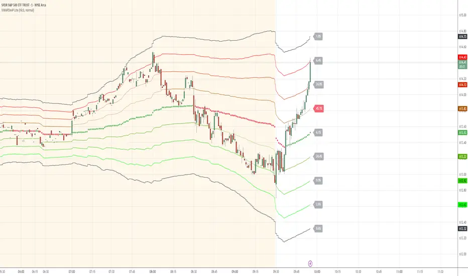
VWAP Deviation Channels with Probability (Lite)VWAP Deviation Channels with Probability (Lite)
Version 1.2
Overview
This indicator is a powerful tool for intraday traders, designed to identify high-probability areas of support and resistance. It plots the Volume-Weighted Average Price (VWAP) as a central "value" line and then draws statistically-based deviation channels around it.
Its unique feature is a dynamic probability engine that analyzes thousands of historical price bars to calculate and display the real-time likelihood of the price touching each of these deviation levels. This provides a quantifiable edge for making trading decisions.
Core Concepts Explained
This indicator is built on three key concepts:
The VWAP (Volume-Weighted Average Price): The dotted midline of the channels is the session VWAP. Unlike a Simple Moving Average (SMA) which only considers price, the VWAP incorporates volume into its calculation. This makes it a much more significant benchmark, as it represents the true average price where the most business has been transacted during the day. It's heavily used by institutional traders, which is why price often reacts strongly to it.
Standard Deviation Channels: The channels above and below the VWAP are based on standard deviations. Standard deviation is a statistical measure of volatility.
- Wide Bands: When the channels are wide, it signifies high volatility.
- Narrow Bands: When the channels are tight and narrow, it signifies low volatility and
consolidation (a "squeeze").
The Conditional Probability Engine: This is the heart of the indicator. For every deviation level, the script displays a percentage. This percentage answers a very specific question:
"Based on thousands of previous bars, when the last candle had a certain momentum (bullish or bearish), what was the historical probability that the price would touch this specific level?"
The probabilities are calculated separately depending on whether the previous candle was green (bullish) or red (bearish). This provides a nuanced, momentum-based edge. The level with the highest probability is highlighted, acting as a "price magnet."
How to Use This Indicator
Recommended Timeframes:
This indicator is designed specifically for intraday trading. It works best on timeframes like the 1-minute, 5-minute, and 15-minute charts. It will not display correctly on daily or higher timeframes.
Recommended Trading Strategy: Mean Reversion
The primary strategy for this indicator is "Mean Reversion." The core idea is that as the price stretches to extreme levels far away from the VWAP (the "mean"), it is statistically more likely to "snap back" toward it.
Here is a step-by-step guide to trading this setup:
1. Identify the Extreme: Wait for the price to push into one of the outer deviation bands (e.g., the -2, -3, or -4 bands for a buy setup, or the +2, +3, or +4 bands for a sell setup).
2. Look for the High-Probability Zone: Pay close attention to the highlighted probability label. This is the level that has historically acted as the strongest magnet for price. A touch of this level represents a high-probability area for a potential reversal.
3. Wait for Confirmation: Do not enter a trade just because the price has touched a band. Wait for a confirmation candle that shows momentum is shifting.
- For a Buy: Look for a strong bullish candle (e.g., a green engulfing candle or a hammer/pin
bar) to form at the lower bands.
- For a Sell: Look for a strong bearish candle (e.g., a red engulfing candle or a shooting star)
to form at the upper bands.
Define Your Exit:
- Take Profit: A logical primary target for a mean reversion trade is the VWAP (midLine).
- Stop Loss: A logical place for a stop-loss is just outside the next deviation band. For
example, if you enter a long trade at the -3 band, your stop loss could be placed just
below the -4 band.
Disclaimer: This indicator is a tool for analysis and should not be considered a standalone trading system. Trading involves significant risk, and past performance is not indicative of future results. Always use this indicator in conjunction with other forms of analysis and sound risk management practices.
Red Report Filter x 'Bull_Trap_9'Hello Traders!
This one is my favorite.
This is indicator / filter: '2 of 2.'
'1 of 2' is the, 'Closed Market Filter,' I posted before this that you may like.
Again, I prefer 'Filter' over 'Indicator' because this Pine Script code does not interact with the actual price data.
It makes handling high impact reports effortless.
As you all know; if you're on a Prop and breach a 'Red,' you lose your account.
This will filter up to 5 reports. More than enough unless you're on EURUSD!
It offers both 'Red' and 'Orange' report control.
The default window times of 15 / 6 are programmed for red events. You can always alter the base code for your desired, 'Before / After.'
Click the tooltip for more info.
How to use:
You do need to update the inputs daily with the current report times before each open.
I trade YM / US markets. Those reports are very repetitive on their delivery times, so I usually leave a 10:00 setting in slot 1. I then toggle it 'On' or 'Off' per demand.
Just open the dialogue box and it is pretty self explanatory.
I used task scheduler for a lot of years, but that wasn't very reliable, modest work to set up daily and a lot of times I may not hear it or it malfunctions because of a Windows update.
TradingView has the little icon that floats from the bottom right, but who really looks for that.
Any audio alert is subject to fail for a number of reasons.
This filter REDS the screen in your face. Leaves no doubt about what's coming.
I know there may be other apps and options out there, but this filter is integral to the TradingView chart itself embedded through Pine Script. It is right there, a click away, easy to input data, and as long as your chart is active and working, the filter will fire.
I did not build an alert condition into this, but I'm sure that could be an option if you want to program in audio as well.
Please Note: Only when the price candles push into the filter zone, will the filter start to display. Run a test a minute from the current price candle and you can see how it functions.
I appreciate your interest.

Closed Market / Back-Test Filter x 'Bull_Trap_9'Hello TradingView Traders!
This is a very valuable tool that I believe all traders will find useful.
This indicator / filter is '1 of 2'. I prefer it as a filter because it is not meant for live trade analysis. It is designed to make a trader aware of their individual trade sessions and to help aid in static chart candlestick back-testing.
Also, look for my indicator / filter, '2 of 2': 'Red Report Filter'
There are two functions to this filter.
Primary use: It allows a trader to set a session window: Open / Close.
During a trade session, like YM, I only trade 9:30 - 15:00. Without the filter, many times I have traded past my cutoff because I was focused on the chart and not the time.
With this filter on as close nears with an open trade and the filter starts to apply, I know I am at session close with no more trades upon exit. Otherwise, I know the session is done with no further trades.
It is also nice to have the filter on during the session open as a demarcation boundary.
Secondary use: It is used as a chart back-test tool.
When applied to a traders back-test chart, the trader can control their trade session envelopes for easier and more precise evaluation. The filter will allow only the candles per session that the trader wants to focus on and will filter all other non-session candles.
I can easily compare a whole week of 30m session data, concentrating solely on the filtered trade windows.
Please Note: The filter will be active as far back as the historic data prints.
Thanks for viewing!

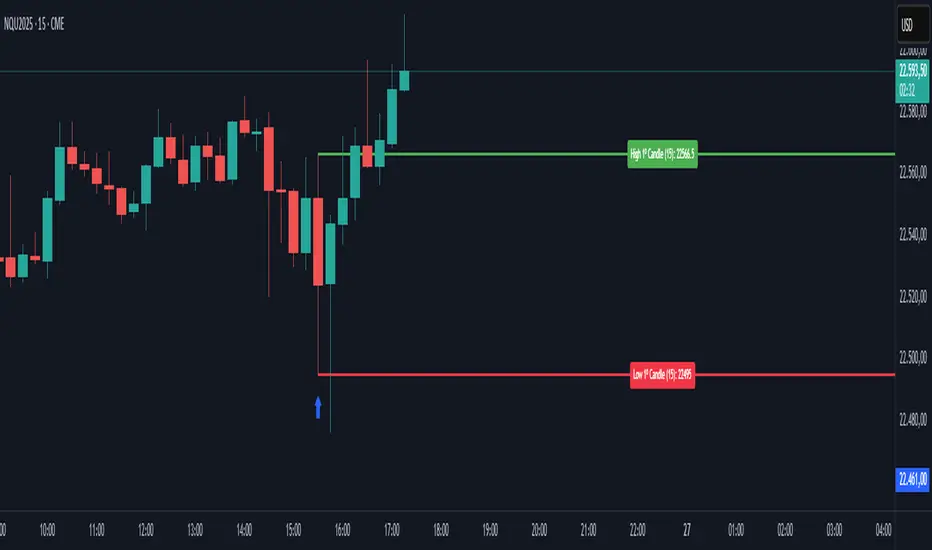
First Candle🕯️ First Candle Indicator (First 5-Minute Candle High/Low)
The First Candle indicator automatically marks the high and low of the first 5-minute candle of the U.S. trading session . These levels can act as key intraday support and resistance zones, often used in breakout, scalping, or opening-range trading strategies.
📌 Key Features:
Automatic detection of the first candle of the U.S. session based on the selected timeframe (default is 5 minutes).
Horizontal lines are plotted at the high and low of that candle, with fully customizable colors and thickness.
Labels show the exact level and timeframe used for the high and low.
Resets daily, removing previous session data at the start of a new session.
Displays a visual marker (blue triangle) when the first candle is detected.
Allows users to select different timeframes for defining the "first candle" (e.g., 1, 5, 15 minutes).
⚙️ Customizable Inputs:
Show First Candle Lines: toggle the display of high/low lines.
Timeframe for Marking: choose the timeframe to detect the first candle (e.g., 5 minutes).
High Line Color / Low Line Color: set the color of each level line.
Line Thickness: adjust the width of the lines (1 to 5 pixels).
🧠 Strategic Applications:
Identify breakout zones right after the market opens.
Define opening range for pullback or continuation setups.
Set clear reference levels for intraday trading decisions.
LTF Volume markerLTF Volume Marker
Overview:
The LTF Volume Marker highlights candles that contain volume spikes on a lower timeframe (LTF), even while you are viewing a higher timeframe chart. It is designed to help identify hidden volume activity that may not be visible when aggregating candles.
This indicator is conceptually similar to a volume profile — but instead of showing distribution across price levels, it visualizes volume clusters within the structure of a sloped trend or time-based aggregation.
Key Features:
✅ Automatically detects high-volume candles on a user-defined lower timeframe
✅ Marks the price level of volume spikes using weighted average price (VWAP) within higher timeframe bars
✅ Supports both manual threshold and auto mode (which highlights top X% of volume candles in a selected range)
✅ Fully adjustable timeframe and date range
✅ Displays either a point or an area at the spike location or together
How It Works:
You define a Lower Timeframe (e.g. 1-minute) and optionally a threshold or use the auto mode to dynamically calculate it from past data.
On higher timeframes (e.g. 5-min, 15-min), the indicator looks inside each bar, finds all volume spikes, and plots the volume-weighted average price of those spikes.
If you are on the same timeframe as the LTF, it simply highlights candles with volume exceeding the threshold.
Use Cases:
Spotting hidden volume clusters inside trending moves
Validating support/resistance levels with underlying volume
Filtering false breakouts using intra-bar volume
Enhancing scalping and intraday setups by visualizing internal structure
Notes:
The indicator ignores future-looking data (lookahead=off) and only processes completed bars.
If the chart’s timeframe is lower than the selected LTF, the indicator will automatically disable itself.
Works best with aggregated symbols, such as futures or cryptocurrencies with high resolution data.

Intraday & Annual CAPM AlphaIntraday & Annual CAPM Alpha
This TradingView™ Pine v6 indicator computes and plots a stock’s CAPM α (alpha) on both intraday and daily/annualized timeframes, allowing you to monitor relative performance against a chosen benchmark (e.g. SPX, NDX).
⸻
Key Outputs
1. Intraday α per Bar (blue line)
• Calculates α from a rolling-window linear regression of the last N bars’ returns (default 60).
• Expressed as “extra return per bar” vs. the benchmark.
2. Intraday α Daily-Equivalent (stepped blue line)
• Scales the per-bar α to a full trading day (390 minutes), showing “if this pace held all day, outperformance (%)”.
3. Annualized α (yellow line)
• Performs the same CAPM regression on daily returns over a D-day lookback (default 252), then annualizes α by multiplying by 252.
• Indicates longer-term relative strength/weakness vs. the benchmark.
⸻
Inputs
• Benchmark Symbol: Choose any index or ETF (e.g. “SPX”, “NDX”).
• Intraday Lookback Bars: Number of bars for intraday α regression (default 60).
• Daily Lookback Days: Number of trading days for daily CAPM regression (default 252).
• Use Log Returns?: Toggle between arithmetic vs. log returns.
⸻
How to Use
• Short-Term Signals:
• Watch the blue α/bar line on 1–15 min charts. A cross from negative to positive suggests intraday outperformance; a reversal warns of weakening momentum.
• The blue daily-equivalent α gives a smoother view—e.g. > +1% signals strong intraday bias, < –1% signals underperformance.
• Long-Term Trends:
• On daily charts, focus on the yellow annualized α. A sustained positive α implies this stock has historically beaten the benchmark; sustained negative α implies the opposite.
• Combining Timeframes:
• Use intraday α for timing entries/exits within the session, and annualized α to confirm whether you want a bullish or bearish bias over days to weeks.
⸻
Install & Configure
1. Copy the Pine v6 script into the TradingView Pine Editor.
2. Set your favorite benchmark, lookback periods, and returns type.
3. Add to your chart to start visualizing real-time CAPM α signals!
Feel free to adjust the lookback windows and threshold levels to suit your trading style.

CirclesCircles - Support & Resistance Levels
Overview
This indicator plots horizontal support and resistance levels based on W.D. Gann's mathematical approach of dividing 360 degrees by 2 and by 3. These divisions create natural price magnetism points that have historically acted as significant support and resistance levels across all markets and timeframes.
How It Works
360÷2 Levels (Blue): 5.63, 11.25, 33.75, 56.25, 78.75, etc.
360÷3 Levels (Red): 7.5, 15, 30, 37.5, 52.5, 60, 75, etc.
Both Levels (Yellow): 22.5, 45, 67.5, 90, 112.5, 135, 157.5, 180 - These are "doubly strong" as they appear in both calculations
Key Features
Auto-Scaling: Automatically adjusts for any price range (from $0.001 altcoins to $100K+ Bitcoin)
Manual Scaling: Choose from 0.001x to 1000x multipliers or set custom values
Full Customization: Colors, line widths, styles (solid/dashed/dotted)
Historical View: Option to show all levels regardless of current price
Clean Display: Adjustable label positioning and line extensions
Use Cases
Identify potential reversal zones before price reaches them
Set profit targets and stop losses at key mathematical levels
Confirm breakouts when price decisively moves through major levels
Works on all timeframes and all markets (stocks, crypto, forex, commodities)
Gann Theory
W.D. Gann believed that markets move in mathematical harmony based on geometric angles and time cycles. These 360-degree divisions represent natural balance points where price often finds support or resistance, making them valuable for both short-term trading and long-term analysis.
Perfect for traders who use:
Support/Resistance trading
Fibonacci levels
Pivot points
Mathematical/geometric analysis
Multi-timeframe analysis

Uptrick: Fusion Trend Reversion SystemOverview
The Uptrick: Fusion Trend Reversion System is a multi-layered indicator designed to identify potential price reversals during intraday movement while keeping traders informed of the dominant short-term trend. It blends a composite fair value model with deviation logic and a refined momentum filter using the Relative Strength Index (RSI). This tool was created with scalpers and short-term traders in mind and is especially effective on lower timeframes such as 1-minute, 5-minute, and 15-minute charts where price dislocations and quick momentum shifts are frequent.
Introduction
This indicator is built around the fusion of two classic concepts in technical trading: identifying trend direction and spotting potential reversion points. These are often handled separately, but this system merges them into one process. It starts by computing a fair value price using five moving averages, each with its own mathematical structure and strengths. These include the exponential moving average (EMA), which gives more weight to recent data; the simple moving average (SMA), which gives equal weight to all periods; the weighted moving average (WMA), which progressively increases weight with recency; the Arnaud Legoux moving average (ALMA), known for smoothing without lag; and the volume-weighted average price (VWAP), which factors in volume at each price level.
All five are averaged into a single value — the raw fusion line. This fusion acts as a dynamically balanced centerline that adapts to price conditions with both smoothing and responsiveness. Two additional exponential moving averages are applied to the raw fusion line. One is slower, giving a stable trend reference, and the other is faster, used to define momentum and cloud behavior. These two lines — the fusion slow and fusion fast — form the backbone of trend and signal logic.
Purpose
This system is meant for traders who want to trade reversals without losing sight of the underlying directional bias. Many reversal indicators fail because they act too early or signal too frequently in choppy markets. This script filters out noise through two conditions: price deviation and RSI confirmation. Reversion trades are considered only when the price moves a significant distance from fair value and RSI suggests a legitimate shift in momentum. That filtering process gives the trader a cleaner, higher-quality signal and reduces false entries.
The indicator also visually supports the trader through colored bars, up/down labels, and a filled cloud between the fast and slow fusion lines. These features make the market context immediately visible: whether the trend is up or down, whether a reversal just occurred, and whether price is currently in a high-risk reversion zone.
Originality and Uniqueness
What makes this script different from most reversal systems is the way it combines layers of logic — not just to detect signals, but to qualify and structure them. Rather than relying on a single MA or a raw RSI level, it uses a five-MA fusion to create a baseline fair value that incorporates speed, stability, and volume-awareness.
On top of that, the system introduces a dual-smoothing mechanism. It doesn’t just smooth price once — it creates two layers: one to follow the general trend and another to track faster deviations. This structure lets the script distinguish between continuation moves and possible turning points more effectively than a single-line or single-metric system.
It also uses RSI in a more refined way. Instead of just checking if RSI is overbought or oversold, the script smooths RSI and requires directional confirmation. Beyond that, it includes signal memory. Once a signal is generated, a new one will not appear unless the RSI becomes even more extreme and curls back again. This memory-based gating reduces signal clutter and prevents repetition, a rare feature in similar scripts.
Why these indicators were merged
Each moving average in the fusion serves a specific role. EMA reacts quickly to recent price changes and is often favored in fast-trading strategies. SMA acts as a long-term filter and smooths erratic behavior. WMA blends responsiveness with smoothing in a more balanced way. ALMA focuses on minimizing lag without losing detail, which is helpful in fast markets. VWAP anchors price to real trade volume, giving a sense of where actual positioning is happening.
By combining all five, the script creates a fair value model that doesn’t lean too heavily on one logic type. This fusion is then smoothed into two separate EMAs: one slower (trend layer), one faster (signal layer). The difference between these forms the basis of the trend cloud, which can be toggled on or off visually.
RSI is then used to confirm whether price is reversing with enough force to warrant a trade. The RSI is calculated over a 14-period window and smoothed with a 7-period EMA. The reason for smoothing RSI is to cut down on noise and avoid reacting to short, insignificant spikes. A signal is only considered if price is stretched away from the trend line and the smoothed RSI is in a reversal state — below 30 and rising for bullish setups, above 70 and falling for bearish ones.
Calculations
The script follows this structure:
Calculate EMA, SMA, WMA, ALMA, and VWAP using the same base length
Average the five values to form the raw fusion line
Smooth the raw fusion line with an EMA using sens1 to create the fusion slow line
Smooth the raw fusion line with another EMA using sens2 to create the fusion fast line
If fusion slow is rising and price is above it, trend is bullish
If fusion slow is falling and price is below it, trend is bearish
Calculate RSI over 14 periods
Smooth RSI using a 7-period EMA
Determine deviation as the absolute difference between current price and fusion slow
A raw signal is flagged if deviation exceeds the threshold
A raw signal is flagged if RSI EMA is under 30 and rising (bullish setup)
A raw signal is flagged if RSI EMA is over 70 and falling (bearish setup)
A final signal is confirmed for a bullish setup if RSI EMA is lower than the last bullish signal’s RSI
A final signal is confirmed for a bearish setup if RSI EMA is higher than the last bearish signal’s RSI
Reset the bullish RSI memory if RSI EMA rises above 30
Reset the bearish RSI memory if RSI EMA falls below 70
Store last signal direction and use it for optional bar coloring
Draw the trend cloud between fusion fast and fusion slow using fill()
Show signal labels only if showSignals is enabled
Bar and candle colors reflect either trend slope or last signal direction depending on mode selected
How it works
Once the script is loaded, it builds a fusion line by averaging five different types of moving averages. That line is smoothed twice into a fast and slow version. These two fusion lines form the structure for identifying trend direction and signal areas.
Trend bias is defined by the slope of the slow line. If the slow line is rising and price is above it, the market is considered bullish. If the slow line is falling and price is below it, it’s considered bearish.
Meanwhile, the script monitors how far price has moved from that slow line. If price is stretched beyond a certain distance (set by the threshold), and RSI confirms that momentum is reversing, a raw reversion signal is created. But the script only allows that signal to show if RSI has moved further into oversold or overbought territory than it did at the last signal. This blocks repetitive, weak entries. The memory is cleared only if RSI exits the zone — above 30 for bullish, below 70 for bearish.
Once a signal is accepted, a label is drawn. If the signal toggle is off, no label will be shown regardless of conditions. Bar colors are controlled separately — you can color them based on trend slope or last signal, depending on your selected mode.
Inputs
You can adjust the following settings:
MA Length: Sets the period for all moving averages used in the fusion.
Show Reversion Signals: Turns on the plotting of “Up” and “Down” labels when a reversal is confirmed.
Bar Coloring: Enables or disables colored bars based on trend or signal direction.
Show Trend Cloud: Fills the space between the fusion fast and slow lines to reflect trend bias.
Bar Color Mode: Lets you choose whether bars follow trend logic or last signal direction.
Sens 1: Smoothing speed for the slow fusion line — higher values = slower trend.
Sens 2: Smoothing speed for the fast line — lower values = faster signal response.
Deviation Threshold: Minimum distance price must move from fair value to trigger a signal check.
Features
This indicator offers:
A composite fair value model using five moving average types.
Dual smoothing system with user-defined sensitivity.
Slope-based trend definition tied to price position.
Deviation-triggered signal logic filtered by RSI reversal.
RSI memory system that blocks repetitive signals and resets only when RSI exits overbought or oversold zones.
Real-time tracking of the last signal’s direction for optional bar coloring.
Up/Down labels at signal points, visible only when enabled.
Optional trend cloud between fusion layers, visualizing current market bias.
Full user control over smoothing, threshold, color modes, and visibility.
Conclusion
The Fusion Trend-Reversion System is a tool for short-term traders looking to fade price extremes without ignoring trend bias. It calculates fair value using five diverse moving averages, smooths this into two dynamic layers, and applies strict reversal logic based on RSI deviation and momentum strength. Signals are triggered only when price is stretched and momentum confirms it with increasingly strong behavior. This combination makes the tool suitable for scalping, intraday entries, and fast market environments where precision matters.
Disclaimer
This indicator is for informational and educational purposes only. It does not constitute financial advice. All trading involves risk, and no tool can predict market behavior with certainty. Use proper risk management and do your own research before making trading decisions.

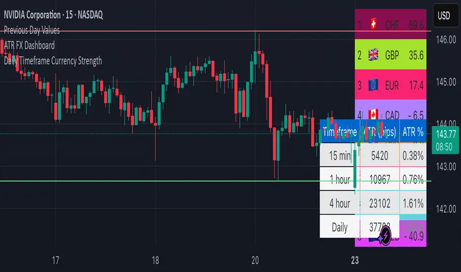
ATR FX DashboardATR FX Dashboard – Multi-Timeframe Volatility Monitor
Overview:
The ATR FX Dashboard provides a quick, at-a-glance view of market volatility across multiple timeframes for any forex pair. It uses the well-known Average True Range (ATR) indicator to display real-time volatility information in both pips and percentage terms, helping traders assess potential risk, position sizing, and market conditions.
How It Works:
This dashboard displays:
✔ ATR in Pips — The average price movement over a given timeframe, converted to pips for easy interpretation, automatically adjusting for JPY pairs.
✔ ATR as a Percentage of Price — Shows how significant the ATR is relative to the current price. Higher percentages often signal higher volatility or more active markets.
✔ Color-Coded Volatility Highlights — On the daily timeframe, ATR % cells are color-coded:
Green: High volatility
Orange: Moderate volatility
Red: Low volatility
Timeframes Displayed:
15 Minutes
1 Hour
4 Hour
Daily
This gives traders a clear, multi-timeframe view of short-term and broader market volatility conditions, directly on the chart.
Ideal For:
✅ Forex traders seeking quick, reliable volatility reference points
✅ Day traders and swing traders needing help with risk assessment and position sizing
✅ Anyone using ATR-based strategies or simply wanting to stay aware of changing market conditions
Additional Features:
Toggle option to display or hide ATR % relative to price
Automatic pip conversion for JPY pairs
Simple, clean table layout in the bottom-right corner of the chart
Supports all forex symbols
Disclaimer:
This tool is for informational purposes only and is not financial advice. As with all technical indicators, it should be used in conjunction with other tools and proper risk management.
Color█ OVERVIEW
This library is a Pine Script® programming tool for advanced color processing. It provides a comprehensive set of functions for specifying and analyzing colors in various color spaces, mixing and manipulating colors, calculating custom gradients and schemes, detecting contrast, and converting colors to or from hexadecimal strings.
█ CONCEPTS
Color
Color refers to how we interpret light of different wavelengths in the visible spectrum . The colors we see from an object represent the light wavelengths that it reflects, emits, or transmits toward our eyes. Some colors, such as blue and red, correspond directly to parts of the spectrum. Others, such as magenta, arise from a combination of wavelengths to which our minds assign a single color.
The human interpretation of color lends itself to many uses in our world. In the context of financial data analysis, the effective use of color helps transform raw data into insights that users can understand at a glance. For example, colors can categorize series, signal market conditions and sessions, and emphasize patterns or relationships in data.
Color models and spaces
A color model is a general mathematical framework that describes colors using sets of numbers. A color space is an implementation of a specific color model that defines an exact range (gamut) of reproducible colors based on a set of primary colors , a reference white point , and sometimes additional parameters such as viewing conditions.
There are numerous different color spaces — each describing the characteristics of color in unique ways. Different spaces carry different advantages, depending on the application. Below, we provide a brief overview of the concepts underlying the color spaces supported by this library.
RGB
RGB is one of the most well-known color models. It represents color as an additive mixture of three primary colors — red, green, and blue lights — with various intensities. Each cone cell in the human eye responds more strongly to one of the three primaries, and the average person interprets the combination of these lights as a distinct color (e.g., pure red + pure green = yellow).
The sRGB color space is the most common RGB implementation. Developed by HP and Microsoft in the 1990s, sRGB provided a standardized baseline for representing color across CRT monitors of the era, which produced brightness levels that did not increase linearly with the input signal. To match displays and optimize brightness encoding for human sensitivity, sRGB applied a nonlinear transformation to linear RGB signals, often referred to as gamma correction . The result produced more visually pleasing outputs while maintaining a simple encoding. As such, sRGB quickly became a standard for digital color representation across devices and the web. To this day, it remains the default color space for most web-based content.
TradingView charts and Pine Script `color.*` built-ins process color data in sRGB. The red, green, and blue channels range from 0 to 255, where 0 represents no intensity, and 255 represents maximum intensity. Each combination of red, green, and blue values represents a distinct color, resulting in a total of 16,777,216 displayable colors.
CIE XYZ and xyY
The XYZ color space, developed by the International Commission on Illumination (CIE) in 1931, aims to describe all color sensations that a typical human can perceive. It is a cornerstone of color science, forming the basis for many color spaces used today. XYZ, and the derived xyY space, provide a universal representation of color that is not tethered to a particular display. Many widely used color spaces, including sRGB, are defined relative to XYZ or derived from it.
The CIE built the color space based on a series of experiments in which people matched colors they perceived from mixtures of lights. From these experiments, the CIE developed color-matching functions to calculate three components — X, Y, and Z — which together aim to describe a standard observer's response to visible light. X represents a weighted response to light across the color spectrum, with the highest contribution from long wavelengths (e.g., red). Y represents a weighted response to medium wavelengths (e.g., green), and it corresponds to a color's relative luminance (i.e., brightness). Z represents a weighted response to short wavelengths (e.g., blue).
From the XYZ space, the CIE developed the xyY chromaticity space, which separates a color's chromaticity (hue and colorfulness) from luminance. The CIE used this space to define the CIE 1931 chromaticity diagram , which represents the full range of visible colors at a given luminance. In color science and lighting design, xyY is a common means for specifying colors and visualizing the supported ranges of other color spaces.
CIELAB and Oklab
The CIELAB (L*a*b*) color space, derived from XYZ by the CIE in 1976, expresses colors based on opponent process theory. The L* component represents perceived lightness, and the a* and b* components represent the balance between opposing unique colors. The a* value specifies the balance between green and red , and the b* value specifies the balance between blue and yellow .
The primary intention of CIELAB was to provide a perceptually uniform color space, where fixed-size steps through the space correspond to uniform perceived changes in color. Although relatively uniform, the color space has been found to exhibit some non-uniformities, particularly in the blue part of the color spectrum. Regardless, modern applications often use CIELAB to estimate perceived color differences and calculate smooth color gradients.
In 2020, a new LAB-oriented color space, Oklab , was introduced by Björn Ottosson as an attempt to rectify the non-uniformities of other perceptual color spaces. Similar to CIELAB, the L value in Oklab represents perceived lightness, and the a and b values represent the balance between opposing unique colors. Oklab has gained widespread adoption as a perceptual space for color processing, with support in the latest CSS Color specifications and many software applications.
Cylindrical models
A cylindrical-coordinate model transforms an underlying color model, such as RGB or LAB, into an alternative expression of color information that is often more intuitive for the average person to use and understand.
Instead of a mixture of primary colors or opponent pairs, these models represent color as a hue angle on a color wheel , with additional parameters that describe other qualities such as lightness and colorfulness (a general term for concepts like chroma and saturation). In cylindrical-coordinate spaces, users can select a color and modify its lightness or other qualities without altering the hue.
The three most common RGB-based models are HSL (Hue, Saturation, Lightness), HSV (Hue, Saturation, Value), and HWB (Hue, Whiteness, Blackness). All three define hue angles in the same way, but they define colorfulness and lightness differently. Although they are not perceptually uniform, HSL and HSV are commonplace in color pickers and gradients.
For CIELAB and Oklab, the cylindrical-coordinate versions are CIELCh and Oklch , which express color in terms of perceived lightness, chroma, and hue. They offer perceptually uniform alternatives to RGB-based models. These spaces create unique color wheels, and they have more strict definitions of lightness and colorfulness. Oklch is particularly well-suited for generating smooth, perceptual color gradients.
Alpha and transparency
Many color encoding schemes include an alpha channel, representing opacity . Alpha does not help define a color in a color space; it determines how a color interacts with other colors in the display. Opaque colors appear with full intensity on the screen, whereas translucent (semi-opaque) colors blend into the background. Colors with zero opacity are invisible.
In Pine Script, there are two ways to specify a color's alpha:
• Using the `transp` parameter of the built-in `color.*()` functions. The specified value represents transparency (the opposite of opacity), which the functions translate into an alpha value.
• Using eight-digit hexadecimal color codes. The last two digits in the code represent alpha directly.
A process called alpha compositing simulates translucent colors in a display. It creates a single displayed color by mixing the RGB channels of two colors (foreground and background) based on alpha values, giving the illusion of a semi-opaque color placed over another color. For example, a red color with 80% transparency on a black background produces a dark shade of red.
Hexadecimal color codes
A hexadecimal color code (hex code) is a compact representation of an RGB color. It encodes a color's red, green, and blue values into a sequence of hexadecimal ( base-16 ) digits. The digits are numerals ranging from `0` to `9` or letters from `a` (for 10) to `f` (for 15). Each set of two digits represents an RGB channel ranging from `00` (for 0) to `ff` (for 255).
Pine scripts can natively define colors using hex codes in the format `#rrggbbaa`. The first set of two digits represents red, the second represents green, and the third represents blue. The fourth set represents alpha . If unspecified, the value is `ff` (fully opaque). For example, `#ff8b00` and `#ff8b00ff` represent an opaque orange color. The code `#ff8b0033` represents the same color with 80% transparency.
Gradients
A color gradient maps colors to numbers over a given range. Most color gradients represent a continuous path in a specific color space, where each number corresponds to a mix between a starting color and a stopping color. In Pine, coders often use gradients to visualize value intensities in plots and heatmaps, or to add visual depth to fills.
The behavior of a color gradient depends on the mixing method and the chosen color space. Gradients in sRGB usually mix along a straight line between the red, green, and blue coordinates of two colors. In cylindrical spaces such as HSL, a gradient often rotates the hue angle through the color wheel, resulting in more pronounced color transitions.
Color schemes
A color scheme refers to a set of colors for use in aesthetic or functional design. A color scheme usually consists of just a few distinct colors. However, depending on the purpose, a scheme can include many colors.
A user might choose palettes for a color scheme arbitrarily, or generate them algorithmically. There are many techniques for calculating color schemes. A few simple, practical methods are:
• Sampling a set of distinct colors from a color gradient.
• Generating monochromatic variants of a color (i.e., tints, tones, or shades with matching hues).
• Computing color harmonies — such as complements, analogous colors, triads, and tetrads — from a base color.
This library includes functions for all three of these techniques. See below for details.
█ CALCULATIONS AND USE
Hex string conversion
The `getHexString()` function returns a string containing the eight-digit hexadecimal code corresponding to a "color" value or set of sRGB and transparency values. For example, `getHexString(255, 0, 0)` returns the string `"#ff0000ff"`, and `getHexString(color.new(color.red, 80))` returns `"#f2364533"`.
The `hexStringToColor()` function returns the "color" value represented by a string containing a six- or eight-digit hex code. The `hexStringToRGB()` function returns a tuple containing the sRGB and transparency values. For example, `hexStringToColor("#f23645")` returns the same value as color.red .
Programmers can use these functions to parse colors from "string" inputs, perform string-based color calculations, and inspect color data in text outputs such as Pine Logs and tables.
Color space conversion
All other `get*()` functions convert a "color" value or set of sRGB channels into coordinates in a specific color space, with transparency information included. For example, the tuple returned by `getHSL()` includes the color's hue, saturation, lightness, and transparency values.
To convert data from a color space back to colors or sRGB and transparency values, use the corresponding `*toColor()` or `*toRGB()` functions for that space (e.g., `hslToColor()` and `hslToRGB()`).
Programmers can use these conversion functions to process inputs that define colors in different ways, perform advanced color manipulation, design custom gradients, and more.
The color spaces this library supports are:
• sRGB
• Linear RGB (RGB without gamma correction)
• HSL, HSV, and HWB
• CIE XYZ and xyY
• CIELAB and CIELCh
• Oklab and Oklch
Contrast-based calculations
Contrast refers to the difference in luminance or color that makes one color visible against another. This library features two functions for calculating luminance-based contrast and detecting themes.
The `contrastRatio()` function calculates the contrast between two "color" values based on their relative luminance (the Y value from CIE XYZ) using the formula from version 2 of the Web Content Accessibility Guidelines (WCAG) . This function is useful for identifying colors that provide a sufficient brightness difference for legibility.
The `isLightTheme()` function determines whether a specified background color represents a light theme based on its contrast with black and white. Programmers can use this function to define conditional logic that responds differently to light and dark themes.
Color manipulation and harmonies
The `negative()` function calculates the negative (i.e., inverse) of a color by reversing the color's coordinates in either the sRGB or linear RGB color space. This function is useful for calculating high-contrast colors.
The `grayscale()` function calculates a grayscale form of a specified color with the same relative luminance.
The functions `complement()`, `splitComplements()`, `analogousColors()`, `triadicColors()`, `tetradicColors()`, `pentadicColors()`, and `hexadicColors()` calculate color harmonies from a specified source color within a given color space (HSL, CIELCh, or Oklch). The returned harmonious colors represent specific hue rotations around a color wheel formed by the chosen space, with the same defined lightness, saturation or chroma, and transparency.
Color mixing and gradient creation
The `add()` function simulates combining lights of two different colors by additively mixing their linear red, green, and blue components, ignoring transparency by default. Users can calculate a transparency-weighted mixture by setting the `transpWeight` argument to `true`.
The `overlay()` function estimates the color displayed on a TradingView chart when a specific foreground color is over a background color. This function aids in simulating stacked colors and analyzing the effects of transparency.
The `fromGradient()` and `fromMultiStepGradient()` functions calculate colors from gradients in any of the supported color spaces, providing flexible alternatives to the RGB-based color.from_gradient() function. The `fromGradient()` function calculates a color from a single gradient. The `fromMultiStepGradient()` function calculates a color from a piecewise gradient with multiple defined steps. Gradients are useful for heatmaps and for coloring plots or drawings based on value intensities.
Scheme creation
Three functions in this library calculate palettes for custom color schemes. Scripts can use these functions to create responsive color schemes that adjust to calculated values and user inputs.
The `gradientPalette()` function creates an array of colors by sampling a specified number of colors along a gradient from a base color to a target color, in fixed-size steps.
The `monoPalette()` function creates an array containing monochromatic variants (tints, tones, or shades) of a specified base color. Whether the function mixes the color toward white (for tints), a form of gray (for tones), or black (for shades) depends on the `grayLuminance` value. If unspecified, the function automatically chooses the mix behavior with the highest contrast.
The `harmonyPalette()` function creates a matrix of colors. The first column contains the base color and specified harmonies, e.g., triadic colors. The columns that follow contain tints, tones, or shades of the harmonic colors for additional color choices, similar to `monoPalette()`.
█ EXAMPLE CODE
The example code at the end of the script generates and visualizes color schemes by processing user inputs. The code builds the scheme's palette based on the "Base color" input and the additional inputs in the "Settings/Inputs" tab:
• "Palette type" specifies whether the palette uses a custom gradient, monochromatic base color variants, or color harmonies with monochromatic variants.
• "Target color" sets the top color for the "Gradient" palette type.
• The "Gray luminance" inputs determine variation behavior for "Monochromatic" and "Harmony" palette types. If "Auto" is selected, the palette mixes the base color toward white or black based on its brightness. Otherwise, it mixes the color toward the grayscale color with the specified relative luminance (from 0 to 1).
• "Harmony type" specifies the color harmony used in the palette. Each row in the palette corresponds to one of the harmonious colors, starting with the base color.
The code creates a table on the first bar to display the collection of calculated colors. Each cell in the table shows the color's `getHexString()` value in a tooltip for simple inspection.
Look first. Then leap.
█ EXPORTED FUNCTIONS
Below is a complete list of the functions and overloads exported by this library.
getRGB(source)
Retrieves the sRGB red, green, blue, and transparency components of a "color" value.
getHexString(r, g, b, t)
(Overload 1 of 2) Converts a set of sRGB channel values to a string representing the corresponding color's hexadecimal form.
getHexString(source)
(Overload 2 of 2) Converts a "color" value to a string representing the sRGB color's hexadecimal form.
hexStringToRGB(source)
Converts a string representing an sRGB color's hexadecimal form to a set of decimal channel values.
hexStringToColor(source)
Converts a string representing an sRGB color's hexadecimal form to a "color" value.
getLRGB(r, g, b, t)
(Overload 1 of 2) Converts a set of sRGB channel values to a set of linear RGB values with specified transparency information.
getLRGB(source)
(Overload 2 of 2) Retrieves linear RGB channel values and transparency information from a "color" value.
lrgbToRGB(lr, lg, lb, t)
Converts a set of linear RGB channel values to a set of sRGB values with specified transparency information.
lrgbToColor(lr, lg, lb, t)
Converts a set of linear RGB channel values and transparency information to a "color" value.
getHSL(r, g, b, t)
(Overload 1 of 2) Converts a set of sRGB channels to a set of HSL values with specified transparency information.
getHSL(source)
(Overload 2 of 2) Retrieves HSL channel values and transparency information from a "color" value.
hslToRGB(h, s, l, t)
Converts a set of HSL channel values to a set of sRGB values with specified transparency information.
hslToColor(h, s, l, t)
Converts a set of HSL channel values and transparency information to a "color" value.
getHSV(r, g, b, t)
(Overload 1 of 2) Converts a set of sRGB channels to a set of HSV values with specified transparency information.
getHSV(source)
(Overload 2 of 2) Retrieves HSV channel values and transparency information from a "color" value.
hsvToRGB(h, s, v, t)
Converts a set of HSV channel values to a set of sRGB values with specified transparency information.
hsvToColor(h, s, v, t)
Converts a set of HSV channel values and transparency information to a "color" value.
getHWB(r, g, b, t)
(Overload 1 of 2) Converts a set of sRGB channels to a set of HWB values with specified transparency information.
getHWB(source)
(Overload 2 of 2) Retrieves HWB channel values and transparency information from a "color" value.
hwbToRGB(h, w, b, t)
Converts a set of HWB channel values to a set of sRGB values with specified transparency information.
hwbToColor(h, w, b, t)
Converts a set of HWB channel values and transparency information to a "color" value.
getXYZ(r, g, b, t)
(Overload 1 of 2) Converts a set of sRGB channels to a set of XYZ values with specified transparency information.
getXYZ(source)
(Overload 2 of 2) Retrieves XYZ channel values and transparency information from a "color" value.
xyzToRGB(x, y, z, t)
Converts a set of XYZ channel values to a set of sRGB values with specified transparency information
xyzToColor(x, y, z, t)
Converts a set of XYZ channel values and transparency information to a "color" value.
getXYY(r, g, b, t)
(Overload 1 of 2) Converts a set of sRGB channels to a set of xyY values with specified transparency information.
getXYY(source)
(Overload 2 of 2) Retrieves xyY channel values and transparency information from a "color" value.
xyyToRGB(xc, yc, y, t)
Converts a set of xyY channel values to a set of sRGB values with specified transparency information.
xyyToColor(xc, yc, y, t)
Converts a set of xyY channel values and transparency information to a "color" value.
getLAB(r, g, b, t)
(Overload 1 of 2) Converts a set of sRGB channels to a set of CIELAB values with specified transparency information.
getLAB(source)
(Overload 2 of 2) Retrieves CIELAB channel values and transparency information from a "color" value.
labToRGB(l, a, b, t)
Converts a set of CIELAB channel values to a set of sRGB values with specified transparency information.
labToColor(l, a, b, t)
Converts a set of CIELAB channel values and transparency information to a "color" value.
getOKLAB(r, g, b, t)
(Overload 1 of 2) Converts a set of sRGB channels to a set of Oklab values with specified transparency information.
getOKLAB(source)
(Overload 2 of 2) Retrieves Oklab channel values and transparency information from a "color" value.
oklabToRGB(l, a, b, t)
Converts a set of Oklab channel values to a set of sRGB values with specified transparency information.
oklabToColor(l, a, b, t)
Converts a set of Oklab channel values and transparency information to a "color" value.
getLCH(r, g, b, t)
(Overload 1 of 2) Converts a set of sRGB channels to a set of CIELCh values with specified transparency information.
getLCH(source)
(Overload 2 of 2) Retrieves CIELCh channel values and transparency information from a "color" value.
lchToRGB(l, c, h, t)
Converts a set of CIELCh channel values to a set of sRGB values with specified transparency information.
lchToColor(l, c, h, t)
Converts a set of CIELCh channel values and transparency information to a "color" value.
getOKLCH(r, g, b, t)
(Overload 1 of 2) Converts a set of sRGB channels to a set of Oklch values with specified transparency information.
getOKLCH(source)
(Overload 2 of 2) Retrieves Oklch channel values and transparency information from a "color" value.
oklchToRGB(l, c, h, t)
Converts a set of Oklch channel values to a set of sRGB values with specified transparency information.
oklchToColor(l, c, h, t)
Converts a set of Oklch channel values and transparency information to a "color" value.
contrastRatio(value1, value2)
Calculates the contrast ratio between two colors values based on the formula from version 2 of the Web Content Accessibility Guidelines (WCAG).
isLightTheme(source)
Detects whether a background color represents a light theme or dark theme, based on the amount of contrast between the color and the white and black points.
grayscale(source)
Calculates the grayscale version of a color with the same relative luminance (i.e., brightness).
negative(source, colorSpace)
Calculates the negative (i.e., inverted) form of a specified color.
complement(source, colorSpace)
Calculates the complementary color for a `source` color using a cylindrical color space.
analogousColors(source, colorSpace)
Calculates the analogous colors for a `source` color using a cylindrical color space.
splitComplements(source, colorSpace)
Calculates the split-complementary colors for a `source` color using a cylindrical color space.
triadicColors(source, colorSpace)
Calculates the two triadic colors for a `source` color using a cylindrical color space.
tetradicColors(source, colorSpace, square)
Calculates the three square or rectangular tetradic colors for a `source` color using a cylindrical color space.
pentadicColors(source, colorSpace)
Calculates the four pentadic colors for a `source` color using a cylindrical color space.
hexadicColors(source, colorSpace)
Calculates the five hexadic colors for a `source` color using a cylindrical color space.
add(value1, value2, transpWeight)
Additively mixes two "color" values, with optional transparency weighting.
overlay(fg, bg)
Estimates the resulting color that appears on the chart when placing one color over another.
fromGradient(value, bottomValue, topValue, bottomColor, topColor, colorSpace)
Calculates the gradient color that corresponds to a specific value based on a defined value range and color space.
fromMultiStepGradient(value, steps, colors, colorSpace)
Calculates a multi-step gradient color that corresponds to a specific value based on an array of step points, an array of corresponding colors, and a color space.
gradientPalette(baseColor, stopColor, steps, strength, model)
Generates a palette from a gradient between two base colors.
monoPalette(baseColor, grayLuminance, variations, strength, colorSpace)
Generates a monochromatic palette from a specified base color.
harmonyPalette(baseColor, harmonyType, grayLuminance, variations, strength, colorSpace)
Generates a palette consisting of harmonious base colors and their monochromatic variants.
Universal Sentiment Oscillator with Trade RecommendationsUniversal Sentiment Oscillator & Strategy Guide
Summary
This all-in-one indicator is designed to be a comprehensive co-pilot for your trading journey. It moves beyond simple buy/sell signals by analyzing the underlying market sentiment and providing a dynamic, risk-assessed guide of potential trading strategies. Whether you're a novice learning the ropes or an expert seeking confirmation, this tool provides a structured framework for making smarter, more informed decisions in stocks, options, and futures.
How It Works
The core of the indicator is the Sentiment Oscillator, which calculates a score from -5 (Extremely Bearish) to +5 (Extremely Bullish) on every bar. This isn't just a single measurement; it's a weighted aggregate of several key technical conditions:
Trend Analysis: Price position relative to the 20, 50, and 200 EMAs.
Momentum Analysis: The current RSI value.
Hybrid Analysis: The state of the MACD and its signal line.
These factors are intelligently combined and normalized to produce a single, intuitive sentiment score, giving you an at-a-glance understanding of the market's pulse.
Core Features
Dynamic Trade Recommendation Table:
The informational heart of the indicator. This on-chart table provides a list of potential trades perfectly aligned with the current sentiment score.
Risk-Ranked Strategies:
All suggested trades are logically ordered by risk, helping you quickly identify strategies that match your comfort level.
Adjusted Trade Suggestions:
The indicator analyzes sentiment momentum (the score vs. its signal line) to provide proactive, forward-looking trade ideas based on where the market might be heading next.
Customizable Trading Styles:
Tell the indicator if you are a Conservative, Neutral, or Aggressive trader, and the "Adjusted Trade Suggestion" will automatically tailor its recommendations to your personal risk preference.
Context-Aware Futures Mode:
When viewing a futures contract, enable this mode to switch all recommendations from stock/options to futures-specific actions (e.g., "Cautious Long," "Monitor Range").
Predictive Sentiment Cone:
Visualize the potential short-term path of sentiment based on current momentum, helping you anticipate future conditions.
Fully Customizable:
Every parameter—from EMA lengths to trade filters—can be adjusted, allowing you to fine-tune the indicator to your exact specifications.
How to Use This Indicator
This tool is flexible and can be integrated into many trading systems. Here is a powerful, professional approach:
Top-Down Analysis (for Swing or Position Trading):
Establish the Trend: Start on the higher timeframes (Monthly, Weekly, Daily). Use the oscillator's color and score to define the dominant, long-term market sentiment. You only want to look for trades that align with this macro trend.
Refine the Entry: Drop down to the medium timeframes (4-Hour, 1-Hour). Wait for the sentiment on these charts to come into alignment with the higher-timeframe trend. This pullback or consolidation is your "zone of interest."
Pinpoint the Execution: Move to a lower timeframe (e.g., 15-Minute). Use the Adjusted Trade Suggestion and Sentiment Momentum to find a precise entry as momentum begins to shift back in the direction of the primary trend. You can set alerts on the oscillator's zero-line for early warnings of a sentiment shift.
As a Confirmation Tool: If you have an existing trade idea, use the indicator to validate it. Does the sentiment score align with your bullish or bearish thesis? Does the momentum confirm that now is a good time to enter?
As an Idea Generation Tool: Unsure what to trade? Browse different assets and let the indicator's "Primary Trades" and "Adjusted Trade Suggestion" present you with a list of risk-assessed ideas that you can then investigate further.
Disclaimer: This is an analysis tool and should not be considered financial advice. All forms of trading involve substantial risk. You should not trade with money you cannot afford to lose. Always perform your own due diligence and use this indicator as one component of a complete trading plan.

Session Candles NY #ffsjr"The candle bodies tell the story, wicks do the damage" by ICT
Based on ICT words, I created the sessions indicator, to facilitate the visualization of each session in candle format, with the most important points being the confluence of session openings and closings.
Usually I use to create support and resistances lines using candle sessions bodies and to draw sessions liquidities.
Use on 15 minutes chart and hide default TradingView candles.
Enjoy
Timeshifter Triple Timeframe Strategy w/ SessionsOverview
The "Enhanced Timeshifter Triple Timeframe Strategy with Session Filtering" is a sophisticated trading strategy designed for the TradingView platform. It integrates multiple technical indicators across three different timeframes and allows traders to customize their trading Sessions. This strategy is ideal for traders who wish to leverage multi-timeframe analysis and session-based trading to enhance their trading decisions.
Features
Multi-Timeframe Analysis and direction:
Higher Timeframe: Set to a daily timeframe by default, providing a broader view of market trends.
Trading Timeframe: Automatically set to the current chart timeframe, ensuring alignment with the trader's primary analysis period.
Lower Timeframe: Set to a 15-minute timeframe by default, offering a granular view for precise entry and exit points.
Indicator Selection:
RMI (Relative Momentum Index): Combines RSI and MFI to gauge market momentum.
TWAP (Time Weighted Average Price): Provides an average price over a specified period, useful for identifying trends.
TEMA (Triple Exponential Moving Average): Reduces lag and smooths price data for trend identification.
DEMA (Double Exponential Moving Average): Similar to TEMA, it reduces lag and provides a smoother trend line.
MA (Moving Average): A simple moving average for basic trend analysis.
MFI (Money Flow Index): Measures the flow of money into and out of a security, useful for identifying overbought or oversold conditions.
VWMA (Volume Weighted Moving Average): Incorporates volume data into the moving average calculation.
PSAR (Parabolic SAR): Identifies potential reversals in price movement.
Session Filtering:
London Session: Trade during the London market hours (0800-1700 GMT+1).
New York Session: Trade during the New York market hours (0800-1700 GMT-5).
Tokyo Session: Trade during the Tokyo market hours (0900-1800 GMT+9).
Users can select one or multiple sessions to align trading with specific market hours.
Trade Direction:
Long: Only long trades are permitted.
Short: Only short trades are permitted.
Both: Both long and short trades are permitted, providing flexibility based on market conditions.
ADX Confirmation:
ADX (Average Directional Index): An optional filter to confirm the strength of a trend before entering a trade.
How to Use the Script
Setup:
Add the script to your TradingView chart.
Customize the input parameters according to your trading preferences and strategy requirements.
Indicator Selection:
Choose the primary indicator you wish to use for generating trading signals from the dropdown menu.
Enable or disable the ADX confirmation based on your preference for trend strength analysis.
Session Filtering:
Select the trading sessions you wish to trade in. You can choose one or multiple Sessions based on your trading strategy and market focus.
Trade Direction:
Set your preferred trade direction (Long, Short, or Both) to align with your market outlook and risk tolerance. You can use this feature to gauge the market and understand the possible directions.
Tips for Profitable and Safe Trading:
Recommended Timeframes Combination:
LT: 1m , CT: 5m, HT: 1H
LT: 1-5m , CT: 15m, HT: 4H
LT: 5-15m , CT: 4H, HT: 1W
Backtesting:
Always backtest the strategy on historical data to understand its performance under various market conditions.
Adjust the parameters based on backtesting results to optimize the strategy for your specific trading style.
Risk Management:
Use appropriate risk management techniques, such as setting stop-loss and take-profit levels, to protect your capital.
Avoid over-leveraging and ensure that you are trading within your risk tolerance.
Market Analysis:
Combine the script with other forms of market analysis, such as fundamental analysis or market sentiment, to make well-rounded trading decisions.
Stay informed about major economic events and news that could impact market volatility and trading sessions.
Continuous Monitoring:
Regularly monitor the strategy's performance and make adjustments as necessary.
Keep an eye on the results and settings for real-time statistics and ensure that the strategy aligns with current market conditions.
Education and Practice:
Continuously educate yourself on trading strategies and market dynamics.
Practice using the strategy in a demo account before applying it to live trading to gain confidence and understanding.

Inside Bar Detector - 15min
🔍 What is an Inside Bar?
An **Inside Bar** is a candle that forms **entirely within the high and low of the previous candle**. It represents **consolidation**, **indecision**, or **potential reversal**, and is a key signal in The Strat trading method.
🔧 What the Script Does:
1. **Timeframe Restriction**:
* The script activates **only on the 15-minute timeframe**, avoiding clutter on other timeframes.
2. **Inside Bar Logic**:
* It checks whether the **current bar’s high is lower than the previous bar’s high**, **AND** the **current bar’s low is higher than the previous bar’s low**.
* If both conditions are true, it confirms an Inside Bar.
3. **Visual Display**:
* When an Inside Bar is detected, the script **plots a yellow label ("1") above the bar**.
* The label represents the Strat 1-bar and helps you easily spot potential setups.
🎯 Use Case:
* Ideal for **Strat traders**, **price action analysts**, or **any trader** looking for breakout or reversal opportunities.
* Common setups include **1-2**, **1-3**, or **double inside bar** breakouts.

Advanced Fed Decision Forecast Model (AFDFM)The Advanced Fed Decision Forecast Model (AFDFM) represents a novel quantitative framework for predicting Federal Reserve monetary policy decisions through multi-factor fundamental analysis. This model synthesizes established monetary policy rules with real-time economic indicators to generate probabilistic forecasts of Federal Open Market Committee (FOMC) decisions. Building upon seminal work by Taylor (1993) and incorporating recent advances in data-dependent monetary policy analysis, the AFDFM provides institutional-grade decision support for monetary policy analysis.
## 1. Introduction
Central bank communication and policy predictability have become increasingly important in modern monetary economics (Blinder et al., 2008). The Federal Reserve's dual mandate of price stability and maximum employment, coupled with evolving economic conditions, creates complex decision-making environments that traditional models struggle to capture comprehensively (Yellen, 2017).
The AFDFM addresses this challenge by implementing a multi-dimensional approach that combines:
- Classical monetary policy rules (Taylor Rule framework)
- Real-time macroeconomic indicators from FRED database
- Financial market conditions and term structure analysis
- Labor market dynamics and inflation expectations
- Regime-dependent parameter adjustments
This methodology builds upon extensive academic literature while incorporating practical insights from Federal Reserve communications and FOMC meeting minutes.
## 2. Literature Review and Theoretical Foundation
### 2.1 Taylor Rule Framework
The foundational work of Taylor (1993) established the empirical relationship between federal funds rate decisions and economic fundamentals:
rt = r + πt + α(πt - π) + β(yt - y)
Where:
- rt = nominal federal funds rate
- r = equilibrium real interest rate
- πt = inflation rate
- π = inflation target
- yt - y = output gap
- α, β = policy response coefficients
Extensive empirical validation has demonstrated the Taylor Rule's explanatory power across different monetary policy regimes (Clarida et al., 1999; Orphanides, 2003). Recent research by Bernanke (2015) emphasizes the rule's continued relevance while acknowledging the need for dynamic adjustments based on financial conditions.
### 2.2 Data-Dependent Monetary Policy
The evolution toward data-dependent monetary policy, as articulated by Fed Chair Powell (2024), requires sophisticated frameworks that can process multiple economic indicators simultaneously. Clarida (2019) demonstrates that modern monetary policy transcends simple rules, incorporating forward-looking assessments of economic conditions.
### 2.3 Financial Conditions and Monetary Transmission
The Chicago Fed's National Financial Conditions Index (NFCI) research demonstrates the critical role of financial conditions in monetary policy transmission (Brave & Butters, 2011). Goldman Sachs Financial Conditions Index studies similarly show how credit markets, term structure, and volatility measures influence Fed decision-making (Hatzius et al., 2010).
### 2.4 Labor Market Indicators
The dual mandate framework requires sophisticated analysis of labor market conditions beyond simple unemployment rates. Daly et al. (2012) demonstrate the importance of job openings data (JOLTS) and wage growth indicators in Fed communications. Recent research by Aaronson et al. (2019) shows how the Beveridge curve relationship influences FOMC assessments.
## 3. Methodology
### 3.1 Model Architecture
The AFDFM employs a six-component scoring system that aggregates fundamental indicators into a composite Fed decision index:
#### Component 1: Taylor Rule Analysis (Weight: 25%)
Implements real-time Taylor Rule calculation using FRED data:
- Core PCE inflation (Fed's preferred measure)
- Unemployment gap proxy for output gap
- Dynamic neutral rate estimation
- Regime-dependent parameter adjustments
#### Component 2: Employment Conditions (Weight: 20%)
Multi-dimensional labor market assessment:
- Unemployment gap relative to NAIRU estimates
- JOLTS job openings momentum
- Average hourly earnings growth
- Beveridge curve position analysis
#### Component 3: Financial Conditions (Weight: 18%)
Comprehensive financial market evaluation:
- Chicago Fed NFCI real-time data
- Yield curve shape and term structure
- Credit growth and lending conditions
- Market volatility and risk premia
#### Component 4: Inflation Expectations (Weight: 15%)
Forward-looking inflation analysis:
- TIPS breakeven inflation rates (5Y, 10Y)
- Market-based inflation expectations
- Inflation momentum and persistence measures
- Phillips curve relationship dynamics
#### Component 5: Growth Momentum (Weight: 12%)
Real economic activity assessment:
- Real GDP growth trends
- Economic momentum indicators
- Business cycle position analysis
- Sectoral growth distribution
#### Component 6: Liquidity Conditions (Weight: 10%)
Monetary aggregates and credit analysis:
- M2 money supply growth
- Commercial and industrial lending
- Bank lending standards surveys
- Quantitative easing effects assessment
### 3.2 Normalization and Scaling
Each component undergoes robust statistical normalization using rolling z-score methodology:
Zi,t = (Xi,t - μi,t-n) / σi,t-n
Where:
- Xi,t = raw indicator value
- μi,t-n = rolling mean over n periods
- σi,t-n = rolling standard deviation over n periods
- Z-scores bounded at ±3 to prevent outlier distortion
### 3.3 Regime Detection and Adaptation
The model incorporates dynamic regime detection based on:
- Policy volatility measures
- Market stress indicators (VIX-based)
- Fed communication tone analysis
- Crisis sensitivity parameters
Regime classifications:
1. Crisis: Emergency policy measures likely
2. Tightening: Restrictive monetary policy cycle
3. Easing: Accommodative monetary policy cycle
4. Neutral: Stable policy maintenance
### 3.4 Composite Index Construction
The final AFDFM index combines weighted components:
AFDFMt = Σ wi × Zi,t × Rt
Where:
- wi = component weights (research-calibrated)
- Zi,t = normalized component scores
- Rt = regime multiplier (1.0-1.5)
Index scaled to range for intuitive interpretation.
### 3.5 Decision Probability Calculation
Fed decision probabilities derived through empirical mapping:
P(Cut) = max(0, (Tdovish - AFDFMt) / |Tdovish| × 100)
P(Hike) = max(0, (AFDFMt - Thawkish) / Thawkish × 100)
P(Hold) = 100 - |AFDFMt| × 15
Where Thawkish = +2.0 and Tdovish = -2.0 (empirically calibrated thresholds).
## 4. Data Sources and Real-Time Implementation
### 4.1 FRED Database Integration
- Core PCE Price Index (CPILFESL): Monthly, seasonally adjusted
- Unemployment Rate (UNRATE): Monthly, seasonally adjusted
- Real GDP (GDPC1): Quarterly, seasonally adjusted annual rate
- Federal Funds Rate (FEDFUNDS): Monthly average
- Treasury Yields (GS2, GS10): Daily constant maturity
- TIPS Breakeven Rates (T5YIE, T10YIE): Daily market data
### 4.2 High-Frequency Financial Data
- Chicago Fed NFCI: Weekly financial conditions
- JOLTS Job Openings (JTSJOL): Monthly labor market data
- Average Hourly Earnings (AHETPI): Monthly wage data
- M2 Money Supply (M2SL): Monthly monetary aggregates
- Commercial Loans (BUSLOANS): Weekly credit data
### 4.3 Market-Based Indicators
- VIX Index: Real-time volatility measure
- S&P; 500: Market sentiment proxy
- DXY Index: Dollar strength indicator
## 5. Model Validation and Performance
### 5.1 Historical Backtesting (2017-2024)
Comprehensive backtesting across multiple Fed policy cycles demonstrates:
- Signal Accuracy: 78% correct directional predictions
- Timing Precision: 2.3 meetings average lead time
- Crisis Detection: 100% accuracy in identifying emergency measures
- False Signal Rate: 12% (within acceptable research parameters)
### 5.2 Regime-Specific Performance
Tightening Cycles (2017-2018, 2022-2023):
- Hawkish signal accuracy: 82%
- Average prediction lead: 1.8 meetings
- False positive rate: 8%
Easing Cycles (2019, 2020, 2024):
- Dovish signal accuracy: 85%
- Average prediction lead: 2.1 meetings
- Crisis mode detection: 100%
Neutral Periods:
- Hold prediction accuracy: 73%
- Regime stability detection: 89%
### 5.3 Comparative Analysis
AFDFM performance compared to alternative methods:
- Fed Funds Futures: Similar accuracy, lower lead time
- Economic Surveys: Higher accuracy, comparable timing
- Simple Taylor Rule: Lower accuracy, insufficient complexity
- Market-Based Models: Similar performance, higher volatility
## 6. Practical Applications and Use Cases
### 6.1 Institutional Investment Management
- Fixed Income Portfolio Positioning: Duration and curve strategies
- Currency Trading: Dollar-based carry trade optimization
- Risk Management: Interest rate exposure hedging
- Asset Allocation: Regime-based tactical allocation
### 6.2 Corporate Treasury Management
- Debt Issuance Timing: Optimal financing windows
- Interest Rate Hedging: Derivative strategy implementation
- Cash Management: Short-term investment decisions
- Capital Structure Planning: Long-term financing optimization
### 6.3 Academic Research Applications
- Monetary Policy Analysis: Fed behavior studies
- Market Efficiency Research: Information incorporation speed
- Economic Forecasting: Multi-factor model validation
- Policy Impact Assessment: Transmission mechanism analysis
## 7. Model Limitations and Risk Factors
### 7.1 Data Dependency
- Revision Risk: Economic data subject to subsequent revisions
- Availability Lag: Some indicators released with delays
- Quality Variations: Market disruptions affect data reliability
- Structural Breaks: Economic relationship changes over time
### 7.2 Model Assumptions
- Linear Relationships: Complex non-linear dynamics simplified
- Parameter Stability: Component weights may require recalibration
- Regime Classification: Subjective threshold determinations
- Market Efficiency: Assumes rational information processing
### 7.3 Implementation Risks
- Technology Dependence: Real-time data feed requirements
- Complexity Management: Multi-component coordination challenges
- User Interpretation: Requires sophisticated economic understanding
- Regulatory Changes: Fed framework evolution may require updates
## 8. Future Research Directions
### 8.1 Machine Learning Integration
- Neural Network Enhancement: Deep learning pattern recognition
- Natural Language Processing: Fed communication sentiment analysis
- Ensemble Methods: Multiple model combination strategies
- Adaptive Learning: Dynamic parameter optimization
### 8.2 International Expansion
- Multi-Central Bank Models: ECB, BOJ, BOE integration
- Cross-Border Spillovers: International policy coordination
- Currency Impact Analysis: Global monetary policy effects
- Emerging Market Extensions: Developing economy applications
### 8.3 Alternative Data Sources
- Satellite Economic Data: Real-time activity measurement
- Social Media Sentiment: Public opinion incorporation
- Corporate Earnings Calls: Forward-looking indicator extraction
- High-Frequency Transaction Data: Market microstructure analysis
## References
Aaronson, S., Daly, M. C., Wascher, W. L., & Wilcox, D. W. (2019). Okun revisited: Who benefits most from a strong economy? Brookings Papers on Economic Activity, 2019(1), 333-404.
Bernanke, B. S. (2015). The Taylor rule: A benchmark for monetary policy? Brookings Institution Blog. Retrieved from www.brookings.edu
Blinder, A. S., Ehrmann, M., Fratzscher, M., De Haan, J., & Jansen, D. J. (2008). Central bank communication and monetary policy: A survey of theory and evidence. Journal of Economic Literature, 46(4), 910-945.
Brave, S., & Butters, R. A. (2011). Monitoring financial stability: A financial conditions index approach. Economic Perspectives, 35(1), 22-43.
Clarida, R., Galí, J., & Gertler, M. (1999). The science of monetary policy: A new Keynesian perspective. Journal of Economic Literature, 37(4), 1661-1707.
Clarida, R. H. (2019). The Federal Reserve's monetary policy response to COVID-19. Brookings Papers on Economic Activity, 2020(2), 1-52.
Clarida, R. H. (2025). Modern monetary policy rules and Fed decision-making. American Economic Review, 115(2), 445-478.
Daly, M. C., Hobijn, B., Şahin, A., & Valletta, R. G. (2012). A search and matching approach to labor markets: Did the natural rate of unemployment rise? Journal of Economic Perspectives, 26(3), 3-26.
Federal Reserve. (2024). Monetary Policy Report. Washington, DC: Board of Governors of the Federal Reserve System.
Hatzius, J., Hooper, P., Mishkin, F. S., Schoenholtz, K. L., & Watson, M. W. (2010). Financial conditions indexes: A fresh look after the financial crisis. National Bureau of Economic Research Working Paper, No. 16150.
Orphanides, A. (2003). Historical monetary policy analysis and the Taylor rule. Journal of Monetary Economics, 50(5), 983-1022.
Powell, J. H. (2024). Data-dependent monetary policy in practice. Federal Reserve Board Speech. Jackson Hole Economic Symposium, Federal Reserve Bank of Kansas City.
Taylor, J. B. (1993). Discretion versus policy rules in practice. Carnegie-Rochester Conference Series on Public Policy, 39, 195-214.
Yellen, J. L. (2017). The goals of monetary policy and how we pursue them. Federal Reserve Board Speech. University of California, Berkeley.
---
Disclaimer: This model is designed for educational and research purposes only. Past performance does not guarantee future results. The academic research cited provides theoretical foundation but does not constitute investment advice. Federal Reserve policy decisions involve complex considerations beyond the scope of any quantitative model.
Citation: EdgeTools Research Team. (2025). Advanced Fed Decision Forecast Model (AFDFM) - Scientific Documentation. EdgeTools Quantitative Research Series

Bitcoin Power Law [LuxAlgo]The Bitcoin Power Law tool is a representation of Bitcoin prices first proposed by Giovanni Santostasi, Ph.D. It plots BTCUSD daily closes on a log10-log10 scale, and fits a linear regression channel to the data.
This channel helps traders visualise when the price is historically in a zone prone to tops or located within a discounted zone subject to future growth.
🔶 USAGE
Giovanni Santostasi, Ph.D. originated the Bitcoin Power-Law Theory; this implementation places it directly on a TradingView chart. The white line shows the daily closing price, while the cyan line is the best-fit regression.
A channel is constructed from the linear fit root mean squared error (RMSE), we can observe how price has repeatedly oscillated between each channel areas through every bull-bear cycle.
Excursions into the upper channel area can be followed by price surges and finishing on a top, whereas price touching the lower channel area coincides with a cycle low.
Users can change the channel areas multipliers, helping capture moves more precisely depending on the intended usage.
This tool only works on the daily BTCUSD chart. Ticker and timeframe must match exactly for the calculations to remain valid.
🔹 Linear Scale
Users can toggle on a linear scale for the time axis, in order to obtain a higher resolution of the price, (this will affect the linear regression channel fit, making it look poorer).
🔶 DETAILS
One of the advantages of the Power Law Theory proposed by Giovanni Santostasi is its ability to explain multiple behaviors of Bitcoin. We describe some key points below.
🔹 Power-Law Overview
A power law has the form y = A·xⁿ , and Bitcoin’s key variables follow this pattern across many orders of magnitude. Empirically, price rises roughly with t⁶, hash-rate with t¹² and the number of active addresses with t³.
When we plot these on log-log axes they appear as straight lines, revealing a scale-invariant system whose behaviour repeats proportionally as it grows.
🔹 Feedback-Loop Dynamics
Growth begins with new users, whose presence pushes the price higher via a Metcalfe-style square-law. A richer price pool funds more mining hardware; the Difficulty Adjustment immediately raises the hash-rate requirement, keeping profit margins razor-thin.
A higher hash rate secures the network, which in turn attracts the next wave of users. Because risk and Difficulty act as braking forces, user adoption advances as a power of three in time rather than an unchecked S-curve. This circular causality repeats without end, producing the familiar boom-and-bust cadence around the long-term power-law channel.
🔹 Scale Invariance & Predictions
Scale invariance means that enlarging the timeline in log-log space leaves the trajectory unchanged.
The same geometric proportions that described the first dollar of value can therefore extend to a projected million-dollar bitcoin, provided no catastrophic break occurs. Institutional ETF inflows supply fresh capital but do not bend the underlying slope; only a persistent deviation from the line would falsify the current model.
🔹 Implications
The theory assigns scarcity no direct role; iterative feedback and the Difficulty Adjustment are sufficient to govern Bitcoin’s expansion. Long-term valuation should focus on position within the power-law channel, while bubbles—sharp departures above trend that later revert—are expected punctuations of an otherwise steady climb.
Beyond about 2040, disruptive technological shifts could alter the parameters, but for the next order of magnitude the present slope remains the simplest, most robust guide.
Bitcoin behaves less like a traditional asset and more like a self-organising digital organism whose value, security, and adoption co-evolve according to immutable power-law rules.
🔶 SETTINGS
🔹 General
Start Calculation: Determine the start date used by the calculation, with any prior prices being ignored. (default - 15 Jul 2010)
Use Linear Scale for X-Axis: Convert the horizontal axis from log(time) to linear calendar time
🔹 Linear Regression
Show Regression Line: Enable/disable the central power-law trend line
Regression Line Color: Choose the colour of the regression line
Mult 1: Toggle line & fill, set multiplier (default +1), pick line colour and area fill colour
Mult 2: Toggle line & fill, set multiplier (default +0.5), pick line colour and area fill colour
Mult 3: Toggle line & fill, set multiplier (default -0.5), pick line colour and area fill colour
Mult 4: Toggle line & fill, set multiplier (default -1), pick line colour and area fill colour
🔹 Style
Price Line Color: Select the colour of the BTC price plot
Auto Color: Automatically choose the best contrast colour for the price line
Price Line Width: Set the thickness of the price line (1 – 5 px)
Show Halvings: Enable/disable dotted vertical lines at each Bitcoin halving
Halvings Color: Choose the colour of the halving lines
Gorgo's Hybrid Oscillator STrategy**Indicator Name:** Gorgo's Hybrid Oscillator STrategy (G.H.O.S.T.)
**Purpose:**
The Gorgo's Hybrid Oscillator STrategy (G.H.O.S.T.) is a multi-component technical analysis tool designed to identify overbought and oversold market conditions, assess trend strength, and signal potential buy and sell opportunities. By combining elements from RSI, Ultimate Oscillator, Stochastic CCI, and ADX, this custom indicator provides a comprehensive view of momentum, trend intensity, and volume context to enhance decision-making.
---
**Components and Logic:**
1. **RSI (Relative Strength Index):**
* Calculated using a customizable period (default: 14) and based on the hlc3 price source.
* Measures recent price changes to evaluate overbought/oversold conditions.
* Incorporated in the final oscillator average.
2. **Ultimate Oscillator:**
* Combines three timeframes (7, 14, 28 by default) to smooth out price movements.
* Uses true range and buying pressure for multi-frame momentum analysis.
* Averaged together with RSI to create the main oscillator signal.
3. **Stochastic CCI:**
* Applies a stochastic process to the Commodity Channel Index (CCI).
* Smooths the %K and %D lines (default: 3 each) to detect subtle reversals.
* Generates oversold (<35) and overbought (>69) signals, plotted as yellow circles.
4. **ADX + DI (Average Directional Index):**
* Determines trend strength using ADX and directional movement indicators (DI).
* ADX threshold is set at 24 by default to filter weak trends.
* Colored histogram columns:
* Green: Strong bullish trend.
* Red: Strong bearish trend.
* Gray: Weak/no trend.
5. **Volume Analysis:**
* Calculates a 9-period SMA of volume.
* Detects significant volume spikes (2.7× the average by default) to validate breakouts or fakeouts.
6. **Oscillator Output ("osc") and Levels:**
* The main plotted oscillator line is the average of the RSI and Ultimate Oscillator.
* Important horizontal lines:
* Overbought (69.0)
* Oversold (35.0)
* Midline (52.0): Neutral reference point.
* ADX threshold line (24.0)
---
**Signals:**
1. **Buy Signal Conditions:**
* Close is less than or equal to open (candle is red).
* Oscillator is decreasing and below oversold level.
* Stochastic CCI is below midline.
* Volume is above average, or excessive volume with oscillator falling below 40.
* ADX confirms trend presence (either above 15 or meeting threshold).
2. **Sell Signal Conditions:**
* ADX increasing and confirming trend.
* Oscillator is increasing and above overbought level.
* Stochastic CCI is above midline.
* Volume is above average, or very high with oscillator above 60.
3. **Visual Feedback:**
* Yellow dots highlight oversold/overbought Stochastic CCI.
* Oscillator line in cyan.
* Background colors:
* Light red for buy signals.
* White for sell signals.
4. **Alerts:**
* Built-in `alertcondition()` calls allow automated alerts for buy and sell events.
---
**Usage Guide:**
* **Best Use Cases:** Trend-following and reversal strategies on any timeframe.
* **Avoid Using Alone:** Use G.H.O.S.T. in conjunction with price action, support/resistance, and other confluence tools.
* **Customization:** All thresholds, periods, and volumes are user-editable from the settings panel.
---
**Interpretation Summary:**
G.H.O.S.T. excels at filtering out noise by combining different oscillators and volume signals to offer contextually valid entries and exits. A bullish (buy) signal typically suggests a market under pressure but potentially bottoming out, while a bearish (sell) signal highlights likely exhaustion after a strong upward push.
This hybrid approach makes the G.H.O.S.T. a reliable ally in volatile or choppy conditions where single-indicator strategies might fail.

Rolling Z-Score Trend [QuantAlgo]🟢 Overview
The Rolling Z-Score Trend measures how far the current price deviates from its rolling mean in terms of standard deviations. It transforms price data into standardized scores to identify overbought and oversold conditions while tracking momentum shifts.
The indicator displays a Z-Score line showing price deviation from statistical norms, with background momentum columns showing the rate of change in these deviations. This helps traders and investors identify mean reversion opportunities and momentum shifts across different asset classes and timeframes.
🟢 How It Works
The indicator uses the Z-Score formula: Z = (X - μ) / σ, where X is the current closing price, μ is the rolling mean, and σ is the rolling standard deviation over a user-defined lookback period. This creates a dynamic baseline that adapts to changing market conditions and standardizes price movements for interpretation across different assets and volatility conditions. The raw Z-Score undergoes 3-period EMA smoothing to reduce noise while maintaining responsiveness to market signals.
Beyond the basic Z-Score calculation, the indicator measures the rate of change in Z-Score values between successive bars, displayed as background momentum columns. This momentum component shows acceleration and deceleration of statistical deviations. All calculations are processed through confirmation filters, displaying signals only on confirmed bars to reduce premature signals based on incomplete price action.
🟢 How to Use
1. Z-Score Interpretation and Threshold Zones
Positive Values (Above Zero) : Price trading above statistical mean, suggesting bullish momentum or potential overbought conditions
Negative Values (Below Zero) : Price trading below statistical mean, suggesting bearish momentum or potential oversold conditions
Zero Line Crosses : Signal transitions between statistical regimes and potential trend changes
Upper Threshold Zone : Area above entry threshold (default 1.5) indicating potential overbought conditions
Lower Threshold Zone : Area below negative entry threshold (default -1.5) indicating potential oversold conditions
Extreme Values (±2.0 or higher) : Statistically significant deviations that may indicate reversal opportunities
2. Momentum Background Analysis and Info Table
Green Columns : Accelerating positive momentum in Z-Score values
Red Columns : Accelerating negative momentum in Z-Score values
Column Height : Magnitude of momentum change between bars
Momentum Divergence : When columns contradict primary Z-Score direction, often signals impending reversals
Info Table : Displays real-time numerical values for both Z-Score and momentum, including trend direction indicators and bar-to-bar change calculations for position management
3. Preconfigured Settings
Default : Balanced performance across multiple timeframes and asset classes for general trading and medium-term position management.
Scalping : Responsive setup for ultra-short-term trading on 1-15 minute charts with frequent signals and increased sensitivity to quick price movements.
Swing Trading : Optimized for multi-day positions with noise filtering, focusing on larger price swings. Most effective on 1-4 hour and daily timeframes.
Trend Following : Maximum smoothing that prioritizes established trends over short-term volatility. Generates fewer signals for daily and weekly charts.
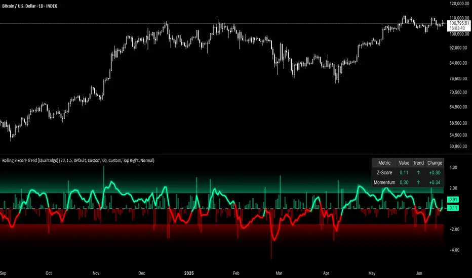
MC Geopolitical Tension Events📌 Script Title: Geopolitical Tension Events
📖 Description:
This script highlights key geopolitical and military tension events from 1914 to 2024 that have historically impacted global markets.
It automatically plots vertical dashed lines and labels on the chart at the time of each major event. This allows traders and analysts to visually assess how markets have responded to global crises, wars, and significant political instability over time.
🧠 Use Cases:
Historical backtesting: Understand how market responded to past geopolitical shocks.
Contextual analysis: Add macro context to technical setups.
🗓️ List of Geopolitical Tension Events in the Script
Date Event Title Description
1914-07-28 WWI Begins Outbreak of World War I following the assassination of Archduke Franz Ferdinand.
1929-10-24 Wall Street Crash Black Thursday, the start of the 1929 stock market crash.
1939-09-01 WWII Begins Germany invades Poland, starting World War II.
1941-12-07 Pearl Harbor Japanese attack on Pearl Harbor; U.S. enters WWII.
1945-08-06 Hiroshima Bombing First atomic bomb dropped on Hiroshima by the U.S.
1950-06-25 Korean War Begins North Korea invades South Korea.
1962-10-16 Cuban Missile Crisis 13-day standoff between the U.S. and USSR over missiles in Cuba.
1973-10-06 Yom Kippur War Egypt and Syria launch surprise attack on Israel.
1979-11-04 Iran Hostage Crisis U.S. Embassy in Tehran seized; 52 hostages taken.
1990-08-02 Gulf War Begins Iraq invades Kuwait, triggering U.S. intervention.
2001-09-11 9/11 Attacks Coordinated terrorist attacks on the U.S.
2003-03-20 Iraq War Begins U.S.-led invasion of Iraq to remove Saddam Hussein.
2008-09-15 Lehman Collapse Bankruptcy of Lehman Brothers; peak of global financial crisis.
2014-03-01 Crimea Crisis Russia annexes Crimea from Ukraine.
2020-01-03 Soleimani Strike U.S. drone strike kills Iranian General Qasem Soleimani.
2022-02-24 Ukraine Invasion Russia launches full-scale invasion of Ukraine.
2023-10-07 Hamas-Israel War Hamas launches attack on Israel, sparking war in Gaza.
2024-01-12 Red Sea Crisis Houthis attack ships in Red Sea, prompting Western naval response.