Ultimate JLines & MTF EMA (Configurable, Labels)## Ultimate JLines & MTF EMA (Configurable, Labels) — Script Overview
This Pine Script is a comprehensive, multi-timeframe indicator based on J Trader concepts. It overlays various Exponential Moving Averages (EMAs), VWAP, inside bar highlights, and dynamic labels onto price charts. The script is highly configurable, allowing users to tailor which elements are displayed and how they appear.
### Key Features
#### 1. **Multi-Timeframe JLines**
- **JLines** are pairs of EMAs (default lengths: 72 and 89) calculated on several timeframes:
- 1 minute (1m)
- 3 minutes (3m)
- 5 minutes (5m)
- 1 hour (1h)
- Custom timeframe (user-selectable)
- Each pair can be visualized as individual lines and as a "cloud" (shaded area between the two EMAs).
- Colors and opacity for each timeframe are user-configurable.
#### 2. **200 EMA on Multiple Timeframes**
- Plots the 200-period EMA on selectable timeframes: 1m, 3m, 5m, 15m, and 1h.
- Each can be toggled independently and colored as desired.
#### 3. **9 EMA and VWAP**
- Plots a 9-period EMA, either on the chart’s current timeframe or a user-specified one.
- Plots VWAP (Volume-Weighted Average Price) for additional trend context.
#### 4. **5/15 EMA Cross Cloud (5min)**
- Calculates and optionally displays a shaded "cloud" between the 5-period and 15-period EMAs on the 5-minute chart.
- Highlights bullish (5 EMA above 15 EMA) and bearish (5 EMA below 15 EMA) conditions with different colors.
- Optionally displays the 5 and 15 EMA lines themselves.
#### 5. **Inside Bar Highlighting**
- Highlights bars where the current high is less than or equal to the previous high and the low is greater than or equal to the previous low (inside bars).
- Color is user-configurable.
#### 6. **9 EMA / VWAP Cross Arrows**
- Plots up/down arrows when the 9 EMA crosses above or below the VWAP.
- Arrow colors and visibility are configurable.
#### 7. **Dynamic Labels**
- On the most recent bar, displays labels for each enabled line (EMAs, VWAP), offset to the right for clarity.
- Labels include the timeframe, type, and current value.
### Customization Options
- **Visibility:** Each plot (line, cloud, arrow, label) can be individually toggled on/off.
- **Colors:** All lines, clouds, and arrows can be colored to user preference, including opacity for clouds.
- **Timeframes:** JLines and EMAs can be calculated on different timeframes, including a custom one.
- **Label Text:** Labels dynamically reflect current indicator values and are color-coded to match their lines.
### Technical Implementation Highlights
- **Helper Functions:** Functions abstract away the logic for multi-timeframe EMA calculation.
- **Security Calls:** Uses `request.security` to fetch data from other timeframes, ensuring accurate multi-timeframe plotting.
- **Efficient Label Management:** Deletes old labels and creates new ones only on the last bar to avoid clutter and maintain performance.
- **Conditional Plotting:** All visual elements are conditionally plotted based on user input, making the indicator highly flexible.
### Use Cases
- **Trend Identification:** Multiple EMAs and VWAP help traders quickly identify trend direction and strength across timeframes.
- **Support/Resistance:** 200 EMA and JLines often act as dynamic support/resistance levels.
- **Entry/Exit Signals:** Crosses between 9 EMA and VWAP, as well as 5/15 EMA clouds, can signal potential trade entries or exits.
- **Pattern Recognition:** Inside bar highlights aid in spotting consolidation and breakout patterns.
### Summary Table of Configurable Elements
| Feature | Timeframes | Cloud Option | Label Option | Color Customizable | Description |
|----------------------------|-------------------|--------------|--------------|--------------------|-----------------------------------------------|
| JLines (72/89 EMA) | 1m, 3m, 5m, 1h, Custom | Yes | Yes | Yes | Key trend-following EMAs with cloud fill |
| 200 EMA | 1m, 3m, 5m, 15m, 1h | No | Yes | Yes | Long-term trend indicator |
| 9 EMA | Any | No | Yes | Yes | Short-term trend indicator |
| VWAP | Chart TF | No | Yes | Yes | Volume-weighted average price |
| 5/15 EMA Cloud (5m) | 5m | Yes | No | Yes | Bullish/bearish cloud between 5/15 EMAs |
| Inside Bar Highlight | Chart TF | No | N/A | Yes | Highlights price consolidation |
| 9 EMA / VWAP Cross Arrows | Chart TF | No | N/A | Yes | Marks EMA/VWAP crossovers with arrows |
This script is ideal for traders seeking a robust, multi-timeframe overlay that combines trend, momentum, and pattern signals in a single, highly customizable indicator. I do not advocate to subscribe to JTrades or the system they tout. This is based on my own observations and not a copy of any JTrades scripts. It is open source to allow full transparency.
Cerca negli script per "美国要强买强卖,要求中国购买指定商品,四年还必须买够15万亿?"

Market Zone Analyzer[BullByte]Understanding the Market Zone Analyzer
---
1. Purpose of the Indicator
The Market Zone Analyzer is a Pine Script™ (version 6) indicator designed to streamline market analysis on TradingView. Rather than scanning multiple separate tools, it unifies four core dimensions—trend strength, momentum, price action, and market activity—into a single, consolidated view. By doing so, it helps traders:
• Save time by avoiding manual cross-referencing of disparate signals.
• Reduce decision-making errors that can arise from juggling multiple indicators.
• Gain a clear, reliable read on whether the market is in a bullish, bearish, or sideways phase, so they can more confidently decide to enter, exit, or hold a position.
---
2. Why a Trader Should Use It
• Unified View: Combines all essential market dimensions into one easy-to-read score and dashboard, eliminating the need to piece together signals manually.
• Adaptability: Automatically adjusts its internal weighting for trend, momentum, and price action based on current volatility. Whether markets are choppy or calm, the indicator remains relevant.
• Ease of Interpretation: Outputs a simple “BULLISH,” “BEARISH,” or “SIDEWAYS” label, supplemented by an intuitive on-chart dashboard and an oscillator plot that visually highlights market direction.
• Reliability Features: Built-in smoothing of the net score and hysteresis logic (requiring consecutive confirmations before flips) minimize false signals during noisy or range-bound phases.
---
3. Why These Specific Indicators?
This script relies on a curated set of well-established technical tools, each chosen for its particular strength in measuring one of the four core dimensions:
1. Trend Strength:
• ADX/DMI (Average Directional Index / Directional Movement Index): Measures how strong a trend is, and whether the +DI line is above the –DI line (bullish) or vice versa (bearish).
• Moving Average Slope (Fast MA vs. Slow MA): Compares a shorter-period SMA to a longer-period SMA; if the fast MA sits above the slow MA, it confirms an uptrend, and vice versa for a downtrend.
• Ichimoku Cloud Differential (Senkou A vs. Senkou B): Provides a forward-looking view of trend direction; Senkou A above Senkou B signals bullishness, and the opposite signals bearishness.
2. Momentum:
• Relative Strength Index (RSI): Identifies overbought (above its dynamically calculated upper bound) or oversold (below its lower bound) conditions; changes in RSI often precede price reversals.
• Stochastic %K: Highlights shifts in short-term momentum by comparing closing price to the recent high/low range; values above its upper band signal bullish momentum, below its lower band signal bearish momentum.
• MACD Histogram: Measures the difference between the MACD line and its signal line; a positive histogram indicates upward momentum, a negative histogram indicates downward momentum.
3. Price Action:
• Highest High / Lowest Low (HH/LL) Range: Over a defined lookback period, this captures breakout or breakdown levels. A closing price near the recent highs (with a positive MA slope) yields a bullish score, and near the lows (with a negative MA slope) yields a bearish score.
• Heikin-Ashi Doji Detection: Uses Heikin-Ashi candles to identify indecision or continuation patterns. A small Heikin-Ashi body (doji) relative to recent volatility is scored as neutral; a larger body in the direction of the MA slope is scored bullish or bearish.
• Candle Range Measurement: Compares each candle’s high-low range against its own dynamic band (average range ± standard deviation). Large candles aligning with the prevailing trend score bullish or bearish accordingly; unusually small candles can indicate exhaustion or consolidation.
4. Market Activity:
• Bollinger Bands Width (BBW): Measures the distance between BB upper and lower bands; wide bands indicate high volatility, narrow bands indicate low volatility.
• Average True Range (ATR): Quantifies average price movement (volatility). A sudden spike in ATR suggests a volatile environment, while a contraction suggests calm.
• Keltner Channels Width (KCW): Similar to BBW but uses ATR around an EMA. Provides a second layer of volatility context, confirming or contrasting BBW readings.
• Volume (with Moving Average): Compares current volume to its moving average ± standard deviation. High volume validates strong moves; low volume signals potential lack of conviction.
By combining these tools, the indicator captures trend direction, momentum strength, price-action nuances, and overall market energy, yielding a more balanced and comprehensive assessment than any single tool alone.
---
4. What Makes This Indicator Stand Out
• Multi-Dimensional Analysis: Rather than relying on a lone oscillator or moving average crossover, it simultaneously evaluates trend, momentum, price action, and activity.
• Dynamic Weighting: The relative importance of trend, momentum, and price action adjusts automatically based on real-time volatility (Market Activity State). For example, in highly volatile conditions, trend and momentum signals carry more weight; in calm markets, price action signals are prioritized.
• Stability Mechanisms:
• Smoothing: The net score is passed through a short moving average, filtering out noise, especially on lower timeframes.
• Hysteresis: Both Market Activity State and the final bullish/bearish/sideways zone require two consecutive confirmations before flipping, reducing whipsaw.
• Visual Interpretation: A fully customizable on-chart dashboard displays each sub-indicator’s value, regime, score, and comment, all color-coded. The oscillator plot changes color to reflect the current market zone (green for bullish, red for bearish, gray for sideways) and shows horizontal threshold lines at +2, 0, and –2.
---
5. Recommended Timeframes
• Short-Term (5 min, 15 min): Day traders and scalpers can benefit from rapid signals, but should enable smoothing (and possibly disable hysteresis) to reduce false whipsaws.
• Medium-Term (1 h, 4 h): Swing traders find a balance between responsiveness and reliability. Less smoothing is required here, and the default parameters (e.g., ADX length = 14, RSI length = 14) perform well.
• Long-Term (Daily, Weekly): Position traders tracking major trends can disable smoothing for immediate raw readings, since higher-timeframe noise is minimal. Adjust lookback lengths (e.g., increase adxLength, rsiLength) if desired for slower signals.
Tip: If you keep smoothing off, stick to timeframes of 1 h or higher to avoid excessive signal “chatter.”
---
6. How Scoring Works
A. Individual Indicator Scores
Each sub-indicator is assigned one of three discrete scores:
• +1 if it indicates a bullish condition (e.g., RSI above its dynamically calculated upper bound).
• 0 if it is neutral (e.g., RSI between upper and lower bounds).
• –1 if it indicates a bearish condition (e.g., RSI below its dynamically calculated lower bound).
Examples of individual score assignments:
• ADX/DMI:
• +1 if ADX ≥ adxThreshold and +DI > –DI (strong bullish trend)
• –1 if ADX ≥ adxThreshold and –DI > +DI (strong bearish trend)
• 0 if ADX < adxThreshold (trend strength below threshold)
• RSI:
• +1 if RSI > RSI_upperBound
• –1 if RSI < RSI_lowerBound
• 0 otherwise
• ATR (as part of Market Activity):
• +1 if ATR > (ATR_MA + stdev(ATR))
• –1 if ATR < (ATR_MA – stdev(ATR))
• 0 otherwise
Each of the four main categories shares this same +1/0/–1 logic across their sub-components.
B. Category Scores
Once each sub-indicator reports +1, 0, or –1, these are summed within their categories as follows:
• Trend Score = (ADX score) + (MA slope score) + (Ichimoku differential score)
• Momentum Score = (RSI score) + (Stochastic %K score) + (MACD histogram score)
• Price Action Score = (Highest-High/Lowest-Low score) + (Heikin-Ashi doji score) + (Candle range score)
• Market Activity Raw Score = (BBW score) + (ATR score) + (KC width score) + (Volume score)
Each category’s summed value can range between –3 and +3 (for Trend, Momentum, and Price Action), and between –4 and +4 for Market Activity raw.
C. Market Activity State and Dynamic Weight Adjustments
Rather than contributing directly to the netScore like the other three categories, Market Activity determines how much weight to assign to Trend, Momentum, and Price Action:
1. Compute Market Activity Raw Score by summing BBW, ATR, KCW, and Volume individual scores (each +1/0/–1).
2. Bucket into High, Medium, or Low Activity:
• High if raw Score ≥ 2 (volatile market).
• Low if raw Score ≤ –2 (calm market).
• Medium otherwise.
3. Apply Hysteresis (if enabled): The state only flips after two consecutive bars register the same high/low/medium label.
4. Set Category Weights:
• High Activity: Trend = 50 %, Momentum = 35 %, Price Action = 15 %.
• Low Activity: Trend = 25 %, Momentum = 20 %, Price Action = 55 %.
• Medium Activity: Use the trader’s base weight inputs (e.g., Trend = 40 %, Momentum = 30 %, Price Action = 30 % by default).
D. Calculating the Net Score
5. Normalize Base Weights (so that the sum of Trend + Momentum + Price Action always equals 100 %).
6. Determine Current Weights based on the Market Activity State (High/Medium/Low).
7. Compute Each Category’s Contribution: Multiply (categoryScore) × (currentWeight).
8. Sum Contributions to get the raw netScore (a floating-point value that can exceed ±3 when scores are strong).
9. Smooth the netScore over two bars (if smoothing is enabled) to reduce noise.
10. Apply Hysteresis to the Final Zone:
• If the smoothed netScore ≥ +2, the bar is classified as “Bullish.”
• If the smoothed netScore ≤ –2, the bar is classified as “Bearish.”
• Otherwise, it is “Sideways.”
• To prevent rapid flips, the script requires two consecutive bars in the new zone before officially changing the displayed zone (if hysteresis is on).
E. Thresholds for Zone Classification
• BULLISH: netScore ≥ +2
• BEARISH: netScore ≤ –2
• SIDEWAYS: –2 < netScore < +2
---
7. Role of Volatility (Market Activity State) in Scoring
Volatility acts as a dynamic switch that shifts which category carries the most influence:
1. High Activity (Volatile):
• Detected when at least two sub-scores out of BBW, ATR, KCW, and Volume equal +1.
• The script sets Trend weight = 50 % and Momentum weight = 35 %. Price Action weight is minimized at 15 %.
• Rationale: In volatile markets, strong trending moves and momentum surges dominate, so those signals are more reliable than nuanced candle patterns.
2. Low Activity (Calm):
• Detected when at least two sub-scores out of BBW, ATR, KCW, and Volume equal –1.
• The script sets Price Action weight = 55 %, Trend = 25 %, and Momentum = 20 %.
• Rationale: In quiet, sideways markets, subtle price-action signals (breakouts, doji patterns, small-range candles) are often the best early indicators of a new move.
3. Medium Activity (Balanced):
• Raw Score between –1 and +1 from the four volatility metrics.
• Uses whatever base weights the trader has specified (e.g., Trend = 40 %, Momentum = 30 %, Price Action = 30 %).
Because volatility can fluctuate rapidly, the script employs hysteresis on Market Activity State: a new High or Low state must occur on two consecutive bars before weights actually shift. This avoids constant back-and-forth weight changes and provides more stability.
---
8. Scoring Example (Hypothetical Scenario)
• Symbol: Bitcoin on a 1-hour chart.
• Market Activity: Raw volatility sub-scores show BBW (+1), ATR (+1), KCW (0), Volume (+1) → Total raw Score = +3 → High Activity.
• Weights Selected: Trend = 50 %, Momentum = 35 %, Price Action = 15 %.
• Trend Signals:
• ADX strong and +DI > –DI → +1
• Fast MA above Slow MA → +1
• Ichimoku Senkou A > Senkou B → +1
→ Trend Score = +3
• Momentum Signals:
• RSI above upper bound → +1
• MACD histogram positive → +1
• Stochastic %K within neutral zone → 0
→ Momentum Score = +2
• Price Action Signals:
• Highest High/Lowest Low check yields 0 (close not near extremes)
• Heikin-Ashi doji reading is neutral → 0
• Candle range slightly above upper bound but trend is strong, so → +1
→ Price Action Score = +1
• Compute Net Score (before smoothing):
• Trend contribution = 3 × 0.50 = 1.50
• Momentum contribution = 2 × 0.35 = 0.70
• Price Action contribution = 1 × 0.15 = 0.15
• Raw netScore = 1.50 + 0.70 + 0.15 = 2.35
• Since 2.35 ≥ +2 and hysteresis is met, the final zone is “Bullish.”
Although the netScore lands at 2.35 (Bullish), smoothing might bring it slightly below 2.00 on the first bar (e.g., 1.90), in which case the script would wait for a second consecutive reading above +2 before officially classifying the zone as Bullish (if hysteresis is enabled).
---
9. Correlation Between Categories
The four categories—Trend Strength, Momentum, Price Action, and Market Activity—often reinforce or offset one another. The script takes advantage of these natural correlations:
• Bullish Alignment: If ADX is strong and pointed upward, fast MA is above slow MA, and Ichimoku is positive, that usually coincides with RSI climbing above its upper bound and the MACD histogram turning positive. In such cases, both Trend and Momentum categories generate +1 or +2. Because the Market Activity State is likely High (given the accompanying volatility), Trend and Momentum weights are at their peak, so the netScore quickly crosses into Bullish territory.
• Sideways/Consolidation: During a low-volatility, sideways phase, ADX may fall below its threshold, MAs may flatten, and RSI might hover in the neutral band. However, subtle price-action signals (like a small breakout candle or a Heikin-Ashi candle with a slight bias) can still produce a +1 in the Price Action category. If Market Activity is Low, Price Action’s weight (55 %) can carry enough influence—even if Trend and Momentum are neutral—to push the netScore out of “Sideways” into a mild bullish or bearish bias.
• Opposing Signals: When Trend is bullish but Momentum turns negative (for example, price continues up but RSI rolls over), the two scores can partially cancel. Market Activity may remain Medium, in which case the netScore lingers near zero (Sideways). The trader can then wait for either a clearer momentum shift or a fresh price-action breakout before committing.
By dynamically recognizing these correlations and adjusting weights, the indicator ensures that:
• When Trend and Momentum align (and volatility supports it), the netScore leaps strongly into Bullish or Bearish.
• When Trend is neutral but Price Action shows an early move in a low-volatility environment, Price Action’s extra weight in the Low Activity State can still produce actionable signals.
---
10. Market Activity State & Its Role (Detailed)
The Market Activity State is not a direct category score—it is an overarching context setter for how heavily to trust Trend, Momentum, or Price Action. Here’s how it is derived and applied:
1. Calculate Four Volatility Sub-Scores:
• BBW: Compare the current band width to its own moving average ± standard deviation. If BBW > (BBW_MA + stdev), assign +1 (high volatility); if BBW < (BBW_MA × 0.5), assign –1 (low volatility); else 0.
• ATR: Compare ATR to its moving average ± standard deviation. A spike above the upper threshold is +1; a contraction below the lower threshold is –1; otherwise 0.
• KCW: Same logic as ATR but around the KCW mean.
• Volume: Compare current volume to its volume MA ± standard deviation. Above the upper threshold is +1; below the lower threshold is –1; else 0.
2. Sum Sub-Scores → Raw Market Activity Score: Range between –4 and +4.
3. Assign Market Activity State:
• High Activity: Raw Score ≥ +2 (at least two volatility metrics are strongly spiking).
• Low Activity: Raw Score ≤ –2 (at least two metrics signal unusually low volatility or thin volume).
• Medium Activity: Raw Score is between –1 and +1 inclusive.
4. Hysteresis for Stability:
• If hysteresis is enabled, a new state only takes hold after two consecutive bars confirm the same High, Medium, or Low label.
• This prevents the Market Activity State from bouncing around when volatility is on the fence.
5. Set Category Weights Based on Activity State:
• High Activity: Trend = 50 %, Momentum = 35 %, Price Action = 15 %.
• Low Activity: Trend = 25 %, Momentum = 20 %, Price Action = 55 %.
• Medium Activity: Use trader’s base weights (e.g., Trend = 40 %, Momentum = 30 %, Price Action = 30 %).
6. Impact on netScore: Because category scores (–3 to +3) multiply by these weights, High Activity amplifies the effect of strong Trend and Momentum scores; Low Activity amplifies the effect of Price Action.
7. Market Context Tooltip: The dashboard includes a tooltip summarizing the current state—e.g., “High activity, trend and momentum prioritized,” “Low activity, price action prioritized,” or “Balanced market, all categories considered.”
---
11. Category Weights: Base vs. Dynamic
Traders begin by specifying base weights for Trend Strength, Momentum, and Price Action that sum to 100 %. These apply only when volatility is in the Medium band. Once volatility shifts:
• High Volatility Overrides:
• Trend jumps from its base (e.g., 40 %) to 50 %.
• Momentum jumps from its base (e.g., 30 %) to 35 %.
• Price Action is reduced to 15 %.
Example: If base weights were Trend = 40 %, Momentum = 30 %, Price Action = 30 %, then in High Activity they become 50/35/15. A Trend score of +3 now contributes 3 × 0.50 = +1.50 to netScore; a Momentum +2 contributes 2 × 0.35 = +0.70. In total, Trend + Momentum can easily push netScore above the +2 threshold on its own.
• Low Volatility Overrides:
• Price Action leaps from its base (30 %) to 55 %.
• Trend falls to 25 %, Momentum falls to 20 %.
Why? When markets are quiet, subtle candle breakouts, doji patterns, and small-range expansions tend to foreshadow the next swing more effectively than raw trend readings. A Price Action score of +3 in this state contributes 3 × 0.55 = +1.65, which can carry the netScore toward +2—even if Trend and Momentum are neutral or only mildly positive.
Because these weight shifts happen only after two consecutive bars confirm a High or Low state (if hysteresis is on), the indicator avoids constantly flipping its emphasis during borderline volatility phases.
---
12. Dominant Category Explained
Within the dashboard, a label such as “Trend Dominant,” “Momentum Dominant,” or “Price Action Dominant” appears when one category’s absolute weighted contribution to netScore is the largest. Concretely:
• Compute each category’s weighted contribution = (raw category score) × (current weight).
• Compare the absolute values of those three contributions.
• The category with the highest absolute value is flagged as Dominant for that bar.
Why It Matters:
• Momentum Dominant: Indicates that the combined force of RSI, Stochastic, and MACD (after weighting) is pushing netScore farther than either Trend or Price Action. In practice, it means that short-term sentiment and speed of change are the primary drivers right now, so traders should watch for continued momentum signals before committing to a trade.
• Trend Dominant: Means ADX, MA slope, and Ichimoku (once weighted) outweigh the other categories. This suggests a strong directional move is in place; trend-following entries or confirming pullbacks are likely to succeed.
• Price Action Dominant: Occurs when breakout/breakdown patterns, Heikin-Ashi candle readings, and range expansions (after weighting) are the most influential. This often happens in calmer markets, where subtle shifts in candle structure can foreshadow bigger moves.
By explicitly calling out which category is carrying the most weight at any moment, the dashboard gives traders immediate insight into why the netScore is tilting toward bullish, bearish, or sideways.
---
13. Oscillator Plot: How to Read It
The “Net Score” oscillator sits below the dashboard and visually displays the smoothed netScore as a line graph. Key features:
1. Value Range: In normal conditions it oscillates roughly between –3 and +3, but extreme confluences can push it outside that range.
2. Horizontal Threshold Lines:
• +2 Line (Bullish threshold)
• 0 Line (Neutral midline)
• –2 Line (Bearish threshold)
3. Zone Coloring:
• Green Background (Bullish Zone): When netScore ≥ +2.
• Red Background (Bearish Zone): When netScore ≤ –2.
• Gray Background (Sideways Zone): When –2 < netScore < +2.
4. Dynamic Line Color:
• The plotted netScore line itself is colored green in a Bullish Zone, red in a Bearish Zone, or gray in a Sideways Zone, creating an immediate visual cue.
Interpretation Tips:
• Crossing Above +2: Signals a strong enough combined trend/momentum/price-action reading to classify as Bullish. Many traders wait for a clear crossing plus a confirmation candle before entering a long position.
• Crossing Below –2: Indicates a strong Bearish signal. Traders may consider short or exit strategies.
• Rising Slope, Even Below +2: If netScore climbs steadily from neutral toward +2, it demonstrates building bullish momentum.
• Divergence: If price makes a higher high but the oscillator fails to reach a new high, it can warn of weakening momentum and a potential reversal.
---
14. Comments and Their Necessity
Every sub-indicator (ADX, MA slope, Ichimoku, RSI, Stochastic, MACD, HH/LL, Heikin-Ashi, Candle Range, BBW, ATR, KCW, Volume) generates a short comment that appears in the detailed dashboard. Examples:
• “Strong bullish trend” or “Strong bearish trend” for ADX/DMI
• “Fast MA above slow MA” or “Fast MA below slow MA” for MA slope
• “RSI above dynamic threshold” or “RSI below dynamic threshold” for RSI
• “MACD histogram positive” or “MACD histogram negative” for MACD Hist
• “Price near highs” or “Price near lows” for HH/LL checks
• “Bullish Heikin Ashi” or “Bearish Heikin Ashi” for HA Doji scoring
• “Large range, trend confirmed” or “Small range, trend contradicted” for Candle Range
Additionally, the top-row comment for each category is:
• Trend: “Highly Bullish,” “Highly Bearish,” or “Neutral Trend.”
• Momentum: “Strong Momentum,” “Weak Momentum,” or “Neutral Momentum.”
• Price Action: “Bullish Action,” “Bearish Action,” or “Neutral Action.”
• Market Activity: “Volatile Market,” “Calm Market,” or “Stable Market.”
Reasons for These Comments:
• Transparency: Shows exactly how each sub-indicator contributed to its category score.
• Education: Helps traders learn why a category is labeled bullish, bearish, or neutral, building intuition over time.
• Customization: If, for example, the RSI comment says “RSI neutral” despite an impending trend shift, a trader might choose to adjust RSI length or thresholds.
In the detailed dashboard, hovering over each comment cell also reveals a tooltip with additional context (e.g., “Fast MA above slow MA” or “Senkou A above Senkou B”), helping traders understand the precise rule behind that +1, 0, or –1 assignment.
---
15. Real-Life Example (Consolidated)
• Instrument & Timeframe: Bitcoin (BTCUSD), 1-hour chart.
• Current Market Activity: BBW and ATR both spike (+1 each), KCW is moderately high (+1), but volume is only neutral (0) → Raw Market Activity Score = +2 → State = High Activity (after two bars, if hysteresis is on).
• Category Weights Applied: Trend = 50 %, Momentum = 35 %, Price Action = 15 %.
• Trend Sub-Scores:
1. ADX = 25 (above threshold 20) with +DI > –DI → +1.
2. Fast MA (20-period) sits above Slow MA (50-period) → +1.
3. Ichimoku: Senkou A > Senkou B → +1.
→ Trend Score = +3.
• Momentum Sub-Scores:
4. RSI = 75 (above its moving average +1 stdev) → +1.
5. MACD histogram = +0.15 → +1.
6. Stochastic %K = 50 (mid-range) → 0.
→ Momentum Score = +2.
• Price Action Sub-Scores:
7. Price is not within 1 % of the 20-period high/low and slope = positive → 0.
8. Heikin-Ashi body is slightly larger than stdev over last 5 bars with haClose > haOpen → +1.
9. Candle range is just above its dynamic upper bound but trend is already captured, so → +1.
→ Price Action Score = +2.
• Calculate netScore (before smoothing):
• Trend contribution = 3 × 0.50 = 1.50
• Momentum contribution = 2 × 0.35 = 0.70
• Price Action contribution = 2 × 0.15 = 0.30
• Raw netScore = 1.50 + 0.70 + 0.30 = 2.50 → Immediately classified as Bullish.
• Oscillator & Dashboard Output:
• The oscillator line crosses above +2 and turns green.
• Dashboard displays:
• Trend Regime “BULLISH,” Trend Score = 3, Comment = “Highly Bullish.”
• Momentum Regime “BULLISH,” Momentum Score = 2, Comment = “Strong Momentum.”
• Price Action Regime “BULLISH,” Price Action Score = 2, Comment = “Bullish Action.”
• Market Activity State “High,” Comment = “Volatile Market.”
• Weights: Trend 50 %, Momentum 35 %, Price Action 15 %.
• Dominant Category: Trend (because 1.50 > 0.70 > 0.30).
• Overall Score: 2.50, posCount = (three +1s in Trend) + (two +1s in Momentum) + (two +1s in Price Action) = 7 bullish signals, negCount = 0.
• Final Zone = “BULLISH.”
• The trader sees that both Trend and Momentum are reinforcing each other under high volatility. They might wait one more candle for confirmation but already have strong evidence to consider a long.
---
• .
---
Disclaimer
This indicator is strictly a technical analysis tool and does not constitute financial advice. All trading involves risk, including potential loss of capital. Past performance is not indicative of future results. Traders should:
• Always backtest the “Market Zone Analyzer ” on their chosen symbols and timeframes before committing real capital.
• Combine this tool with sound risk management, position sizing, and, if possible, fundamental analysis.
• Understand that no indicator is foolproof; always be prepared for unexpected market moves.
Goodluck
-BullByte!
---

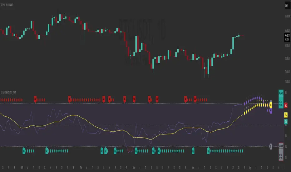
RSI Full Forecast [Titans_Invest]RSI Full Forecast
Get ready to experience the ultimate evolution of RSI-based indicators – the RSI Full Forecast, a boosted and even smarter version of the already powerful: RSI Forecast
Now featuring over 40 additional entry conditions (forecasts), this indicator redefines the way you view the market.
AI-Powered RSI Forecasting:
Using advanced linear regression with the least squares method – a solid foundation for machine learning - the RSI Full Forecast enables you to predict future RSI behavior with impressive accuracy.
But that’s not all: this new version also lets you monitor future crossovers between the RSI and the MA RSI, delivering early and strategic signals that go far beyond traditional analysis.
You’ll be able to monitor future crossovers up to 20 bars ahead, giving you an even broader and more precise view of market movements.
See the Future, Now:
• Track upcoming RSI & RSI MA crossovers in advance.
• Identify potential reversal zones before price reacts.
• Uncover statistical behavior patterns that would normally go unnoticed.
40+ Intelligent Conditions:
The new layer of conditions is designed to detect multiple high-probability scenarios based on historical patterns and predictive modeling. Each additional forecast is a window into the price's future, powered by robust mathematics and advanced algorithmic logic.
Full Customization:
All parameters can be tailored to fit your strategy – from smoothing periods to prediction sensitivity. You have complete control to turn raw data into smart decisions.
Innovative, Accurate, Unique:
This isn’t just an upgrade. It’s a quantum leap in technical analysis.
RSI Full Forecast is the first of its kind: an indicator that blends statistical analysis, machine learning, and visual design to create a true real-time predictive system.
⯁ SCIENTIFIC BASIS LINEAR REGRESSION
Linear Regression is a fundamental method of statistics and machine learning, used to model the relationship between a dependent variable y and one or more independent variables 𝑥.
The general formula for a simple linear regression is given by:
y = β₀ + β₁x + ε
β₁ = Σ((xᵢ - x̄)(yᵢ - ȳ)) / Σ((xᵢ - x̄)²)
β₀ = ȳ - β₁x̄
Where:
y = is the predicted variable (e.g. future value of RSI)
x = is the explanatory variable (e.g. time or bar index)
β0 = is the intercept (value of 𝑦 when 𝑥 = 0)
𝛽1 = is the slope of the line (rate of change)
ε = is the random error term
The goal is to estimate the coefficients 𝛽0 and 𝛽1 so as to minimize the sum of the squared errors — the so-called Random Error Method Least Squares.
⯁ LEAST SQUARES ESTIMATION
To minimize the error between predicted and observed values, we use the following formulas:
β₁ = /
β₀ = ȳ - β₁x̄
Where:
∑ = sum
x̄ = mean of x
ȳ = mean of y
x_i, y_i = individual values of the variables.
Where:
x_i and y_i are the means of the independent and dependent variables, respectively.
i ranges from 1 to n, the number of observations.
These equations guarantee the best linear unbiased estimator, according to the Gauss-Markov theorem, assuming homoscedasticity and linearity.
⯁ LINEAR REGRESSION IN MACHINE LEARNING
Linear regression is one of the cornerstones of supervised learning. Its simplicity and ability to generate accurate quantitative predictions make it essential in AI systems, predictive algorithms, time series analysis, and automated trading strategies.
By applying this model to the RSI, you are literally putting artificial intelligence at the heart of a classic indicator, bringing a new dimension to technical analysis.
⯁ VISUAL INTERPRETATION
Imagine an RSI time series like this:
Time →
RSI →
The regression line will smooth these values and extend them n periods into the future, creating a predicted trajectory based on the historical moment. This line becomes the predicted RSI, which can be crossed with the actual RSI to generate more intelligent signals.
⯁ SUMMARY OF SCIENTIFIC CONCEPTS USED
Linear Regression Models the relationship between variables using a straight line.
Least Squares Minimizes the sum of squared errors between prediction and reality.
Time Series Forecasting Estimates future values based on historical data.
Supervised Learning Trains models to predict outputs from known inputs.
Statistical Smoothing Reduces noise and reveals underlying trends.
⯁ WHY THIS INDICATOR IS REVOLUTIONARY
Scientifically-based: Based on statistical theory and mathematical inference.
Unprecedented: First public RSI with least squares predictive modeling.
Intelligent: Built with machine learning logic.
Practical: Generates forward-thinking signals.
Customizable: Flexible for any trading strategy.
⯁ CONCLUSION
By combining RSI with linear regression, this indicator allows a trader to predict market momentum, not just follow it.
RSI Full Forecast is not just an indicator — it is a scientific breakthrough in technical analysis technology.
⯁ Example of simple linear regression, which has one independent variable:
⯁ In linear regression, observations ( red ) are considered to be the result of random deviations ( green ) from an underlying relationship ( blue ) between a dependent variable ( y ) and an independent variable ( x ).
⯁ Visualizing heteroscedasticity in a scatterplot against 100 random fitted values using Matlab:
⯁ The data sets in the Anscombe's quartet are designed to have approximately the same linear regression line (as well as nearly identical means, standard deviations, and correlations) but are graphically very different. This illustrates the pitfalls of relying solely on a fitted model to understand the relationship between variables.
⯁ The result of fitting a set of data points with a quadratic function:
_________________________________________________
🔮 Linear Regression: PineScript Technical Parameters 🔮
_________________________________________________
Forecast Types:
• Flat: Assumes prices will remain the same.
• Linreg: Makes a 'Linear Regression' forecast for n periods.
Technical Information:
ta.linreg (built-in function)
Linear regression curve. A line that best fits the specified prices over a user-defined time period. It is calculated using the least squares method. The result of this function is calculated using the formula: linreg = intercept + slope * (length - 1 - offset), where intercept and slope are the values calculated using the least squares method on the source series.
Syntax:
• Function: ta.linreg()
Parameters:
• source: Source price series.
• length: Number of bars (period).
• offset: Offset.
• return: Linear regression curve.
This function has been cleverly applied to the RSI, making it capable of projecting future values based on past statistical trends.
______________________________________________________
______________________________________________________
⯁ WHAT IS THE RSI❓
The Relative Strength Index (RSI) is a technical analysis indicator developed by J. Welles Wilder. It measures the magnitude of recent price movements to evaluate overbought or oversold conditions in a market. The RSI is an oscillator that ranges from 0 to 100 and is commonly used to identify potential reversal points, as well as the strength of a trend.
⯁ HOW TO USE THE RSI❓
The RSI is calculated based on average gains and losses over a specified period (usually 14 periods). It is plotted on a scale from 0 to 100 and includes three main zones:
• Overbought: When the RSI is above 70, indicating that the asset may be overbought.
• Oversold: When the RSI is below 30, indicating that the asset may be oversold.
• Neutral Zone: Between 30 and 70, where there is no clear signal of overbought or oversold conditions.
______________________________________________________
______________________________________________________
⯁ ENTRY CONDITIONS
The conditions below are fully flexible and allow for complete customization of the signal.
______________________________________________________
______________________________________________________
🔹 CONDITIONS TO BUY 📈
______________________________________________________
• Signal Validity: The signal will remain valid for X bars .
• Signal Sequence: Configurable as AND or OR .
📈 RSI Conditions:
🔹 RSI > Upper
🔹 RSI < Upper
🔹 RSI > Lower
🔹 RSI < Lower
🔹 RSI > Middle
🔹 RSI < Middle
🔹 RSI > MA
🔹 RSI < MA
📈 MA Conditions:
🔹 MA > Upper
🔹 MA < Upper
🔹 MA > Lower
🔹 MA < Lower
📈 Crossovers:
🔹 RSI (Crossover) Upper
🔹 RSI (Crossunder) Upper
🔹 RSI (Crossover) Lower
🔹 RSI (Crossunder) Lower
🔹 RSI (Crossover) Middle
🔹 RSI (Crossunder) Middle
🔹 RSI (Crossover) MA
🔹 RSI (Crossunder) MA
🔹 MA (Crossover) Upper
🔹 MA (Crossunder) Upper
🔹 MA (Crossover) Lower
🔹 MA (Crossunder) Lower
📈 RSI Divergences:
🔹 RSI Divergence Bull
🔹 RSI Divergence Bear
📈 RSI Forecast:
🔹 RSI (Crossover) MA Forecast
🔹 RSI (Crossunder) MA Forecast
🔹 RSI Forecast 1 > MA Forecast 1
🔹 RSI Forecast 1 < MA Forecast 1
🔹 RSI Forecast 2 > MA Forecast 2
🔹 RSI Forecast 2 < MA Forecast 2
🔹 RSI Forecast 3 > MA Forecast 3
🔹 RSI Forecast 3 < MA Forecast 3
🔹 RSI Forecast 4 > MA Forecast 4
🔹 RSI Forecast 4 < MA Forecast 4
🔹 RSI Forecast 5 > MA Forecast 5
🔹 RSI Forecast 5 < MA Forecast 5
🔹 RSI Forecast 6 > MA Forecast 6
🔹 RSI Forecast 6 < MA Forecast 6
🔹 RSI Forecast 7 > MA Forecast 7
🔹 RSI Forecast 7 < MA Forecast 7
🔹 RSI Forecast 8 > MA Forecast 8
🔹 RSI Forecast 8 < MA Forecast 8
🔹 RSI Forecast 9 > MA Forecast 9
🔹 RSI Forecast 9 < MA Forecast 9
🔹 RSI Forecast 10 > MA Forecast 10
🔹 RSI Forecast 10 < MA Forecast 10
🔹 RSI Forecast 11 > MA Forecast 11
🔹 RSI Forecast 11 < MA Forecast 11
🔹 RSI Forecast 12 > MA Forecast 12
🔹 RSI Forecast 12 < MA Forecast 12
🔹 RSI Forecast 13 > MA Forecast 13
🔹 RSI Forecast 13 < MA Forecast 13
🔹 RSI Forecast 14 > MA Forecast 14
🔹 RSI Forecast 14 < MA Forecast 14
🔹 RSI Forecast 15 > MA Forecast 15
🔹 RSI Forecast 15 < MA Forecast 15
🔹 RSI Forecast 16 > MA Forecast 16
🔹 RSI Forecast 16 < MA Forecast 16
🔹 RSI Forecast 17 > MA Forecast 17
🔹 RSI Forecast 17 < MA Forecast 17
🔹 RSI Forecast 18 > MA Forecast 18
🔹 RSI Forecast 18 < MA Forecast 18
🔹 RSI Forecast 19 > MA Forecast 19
🔹 RSI Forecast 19 < MA Forecast 19
🔹 RSI Forecast 20 > MA Forecast 20
🔹 RSI Forecast 20 < MA Forecast 20
______________________________________________________
______________________________________________________
🔸 CONDITIONS TO SELL 📉
______________________________________________________
• Signal Validity: The signal will remain valid for X bars .
• Signal Sequence: Configurable as AND or OR .
📉 RSI Conditions:
🔸 RSI > Upper
🔸 RSI < Upper
🔸 RSI > Lower
🔸 RSI < Lower
🔸 RSI > Middle
🔸 RSI < Middle
🔸 RSI > MA
🔸 RSI < MA
📉 MA Conditions:
🔸 MA > Upper
🔸 MA < Upper
🔸 MA > Lower
🔸 MA < Lower
📉 Crossovers:
🔸 RSI (Crossover) Upper
🔸 RSI (Crossunder) Upper
🔸 RSI (Crossover) Lower
🔸 RSI (Crossunder) Lower
🔸 RSI (Crossover) Middle
🔸 RSI (Crossunder) Middle
🔸 RSI (Crossover) MA
🔸 RSI (Crossunder) MA
🔸 MA (Crossover) Upper
🔸 MA (Crossunder) Upper
🔸 MA (Crossover) Lower
🔸 MA (Crossunder) Lower
📉 RSI Divergences:
🔸 RSI Divergence Bull
🔸 RSI Divergence Bear
📉 RSI Forecast:
🔸 RSI (Crossover) MA Forecast
🔸 RSI (Crossunder) MA Forecast
🔸 RSI Forecast 1 > MA Forecast 1
🔸 RSI Forecast 1 < MA Forecast 1
🔸 RSI Forecast 2 > MA Forecast 2
🔸 RSI Forecast 2 < MA Forecast 2
🔸 RSI Forecast 3 > MA Forecast 3
🔸 RSI Forecast 3 < MA Forecast 3
🔸 RSI Forecast 4 > MA Forecast 4
🔸 RSI Forecast 4 < MA Forecast 4
🔸 RSI Forecast 5 > MA Forecast 5
🔸 RSI Forecast 5 < MA Forecast 5
🔸 RSI Forecast 6 > MA Forecast 6
🔸 RSI Forecast 6 < MA Forecast 6
🔸 RSI Forecast 7 > MA Forecast 7
🔸 RSI Forecast 7 < MA Forecast 7
🔸 RSI Forecast 8 > MA Forecast 8
🔸 RSI Forecast 8 < MA Forecast 8
🔸 RSI Forecast 9 > MA Forecast 9
🔸 RSI Forecast 9 < MA Forecast 9
🔸 RSI Forecast 10 > MA Forecast 10
🔸 RSI Forecast 10 < MA Forecast 10
🔸 RSI Forecast 11 > MA Forecast 11
🔸 RSI Forecast 11 < MA Forecast 11
🔸 RSI Forecast 12 > MA Forecast 12
🔸 RSI Forecast 12 < MA Forecast 12
🔸 RSI Forecast 13 > MA Forecast 13
🔸 RSI Forecast 13 < MA Forecast 13
🔸 RSI Forecast 14 > MA Forecast 14
🔸 RSI Forecast 14 < MA Forecast 14
🔸 RSI Forecast 15 > MA Forecast 15
🔸 RSI Forecast 15 < MA Forecast 15
🔸 RSI Forecast 16 > MA Forecast 16
🔸 RSI Forecast 16 < MA Forecast 16
🔸 RSI Forecast 17 > MA Forecast 17
🔸 RSI Forecast 17 < MA Forecast 17
🔸 RSI Forecast 18 > MA Forecast 18
🔸 RSI Forecast 18 < MA Forecast 18
🔸 RSI Forecast 19 > MA Forecast 19
🔸 RSI Forecast 19 < MA Forecast 19
🔸 RSI Forecast 20 > MA Forecast 20
🔸 RSI Forecast 20 < MA Forecast 20
______________________________________________________
______________________________________________________
🤖 AUTOMATION 🤖
• You can automate the BUY and SELL signals of this indicator.
______________________________________________________
______________________________________________________
⯁ UNIQUE FEATURES
______________________________________________________
Linear Regression: (Forecast)
Signal Validity: The signal will remain valid for X bars
Signal Sequence: Configurable as AND/OR
Condition Table: BUY/SELL
Condition Labels: BUY/SELL
Plot Labels in the Graph Above: BUY/SELL
Automate and Monitor Signals/Alerts: BUY/SELL
Linear Regression (Forecast)
Signal Validity: The signal will remain valid for X bars
Signal Sequence: Configurable as AND/OR
Condition Table: BUY/SELL
Condition Labels: BUY/SELL
Plot Labels in the Graph Above: BUY/SELL
Automate and Monitor Signals/Alerts: BUY/SELL
______________________________________________________
📜 SCRIPT : RSI Full Forecast
🎴 Art by : @Titans_Invest & @DiFlip
👨💻 Dev by : @Titans_Invest & @DiFlip
🎑 Titans Invest — The Wizards Without Gloves 🧤
✨ Enjoy!
______________________________________________________
o Mission 🗺
• Inspire Traders to manifest Magic in the Market.
o Vision 𐓏
• To elevate collective Energy 𐓷𐓏
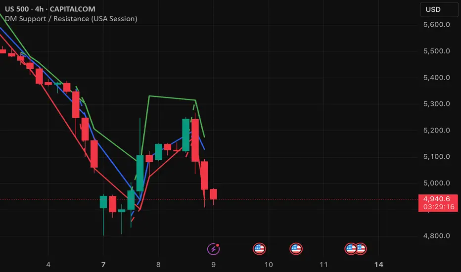
DM Support / Resistance (USA Session)This indicator is specifically designed for use on the 4-hour time frame and helps traders identify key support and resistance levels during the USA trading session (9:30 AM to 4:00 PM Eastern Time). The indicator calculates important price levels to assist in making well-informed entry and exit decisions, particularly for those focusing on swing trades or longer-term intraday strategies. It also includes a feature to skip setups when relevant fundamental news is scheduled, ensuring you avoid trading during periods of high volatility.
Key Features:
Support and Resistance Levels (S1 & R1):
The indicator calculates and displays Support 1 (S1) and Resistance 1 (R1) levels, which act as key barriers for price action and help traders spot potential reversal or breakout zones on the chart.
Pivot Point (PP):
The Pivot Point (PP) is calculated as the average of the previous period's high, low, and close. It serves as a central reference point for market direction, allowing traders to evaluate whether the market is in a bullish or bearish trend.
Market Bias:
The Bias is shown as a histogram that helps traders assess the strength of the market trend. A positive bias suggests bullish sentiment, while a negative bias signals bearish conditions. This can be used to confirm the overall trend direction.
4-Hour Time Frame:
The indicator is optimized for the 4-hour time frame, making it suitable for traders looking for swing trades or those who wish to capture longer-term trends within the USA session. The key support, resistance, and pivot levels are recalculated dynamically to reflect price action over 4-hour periods.
Dynamic Plotting and Alerts:
Support and resistance levels are drawn as dashed horizontal lines, updating in real-time to reflect the most current market data during the USA session. Alerts can be set for significant price movements crossing these levels.
Stop-Loss Strategy Based on 15-Minute Time Frame:
A unique feature of this indicator is its stop-loss strategy, which uses 15-minute time frame support and resistance levels. When a long or short entry is triggered on the 4-hour chart, traders should place their stop-loss according to the relevant 15-minute support or resistance level.
If the price closes above the 15-minute support for a long entry, or closes below the 15-minute resistance for a short entry, it signals the need to exit or adjust your position based on these levels.
Fundamental News Filter:
To avoid unnecessary risk, the indicator incorporates a fundamental news filter. If there is relevant news scheduled during the USA session, such as high-impact economic data or central bank announcements, the indicator will skip the setup for that period. This prevents traders from entering positions during times of elevated volatility caused by news events, which could result in unpredictable price movements.
How to Use:
Long Entry: When the Bias is positive and the price breaks above Support 1 (S1), this signals a potential bullish move. Consider entering a long position at this point.
Stop-Loss Strategy: Set your stop-loss at the respective 15-minute support level. If the price closes below this level, it could signal a reversal, prompting you to exit the trade.
Short Entry: When the Bias is negative and the price breaks below Resistance 1 (R1), this signals a potential bearish move. Enter a short position at this point.
Stop-Loss Strategy: Set your stop-loss at the respective 15-minute resistance level. If the price closes above this level, exit the short trade as it could indicate a bullish reversal.
Pivot Point (PP): The Pivot Point serves as a reference level to gauge potential price reversals. A move above the PP suggests a bullish bias, while trading below the PP suggests a bearish outlook.
Bias Histogram: The Bias Histogram helps confirm trend direction. A positive bias confirms long positions, while a negative bias reinforces short trades.
Avoid Trading During High-Impact News: If there is significant economic news or fundamental events scheduled during the USA session, the indicator will automatically skip any potential setup. This feature ensures you avoid entering trades that might be affected by unexpected news-driven volatility, keeping your trading strategy safer and more reliable.
Why Use This Indicator:
The 4-hour time frame is ideal for traders who prefer swing trading or those looking to capture longer-term trends in a structured manner. This indicator provides crucial insights into market direction, support/resistance levels, and potential entry/exit points.
The stop-loss management based on the 15-minute support and resistance levels helps traders protect their positions from sudden price reversals, ensuring more precise risk management.
The fundamental news filter is particularly useful for avoidance of high-risk periods. By skipping setups during high-impact news events, traders can avoid entering trades when price volatility could be unpredictable.
Overall, this indicator is a powerful tool for traders who want to make data-driven decisions based on technical analysis while ensuring that their positions are managed responsibly and avoiding news-driven risk.
HTF Candle Range Box (Fixed to HTF Bars)### **Higher Timeframe Candle Range Box (HTF Box Indicator)**
This indicator visually highlights the price range of the most recently closed higher-timeframe (HTF) candle, directly on a lower-timeframe chart. It dynamically adjusts based on the user-selected HTF setting (e.g., 15-minute, 1-hour) and ensures that the box is displayed only on the bars that correspond to that specific HTF candle’s duration.
For instance, if a trader is on a **1-minute chart** with the **HTF set to 15 minutes**, the indicator will draw a box spanning exactly 15 one-minute candles, corresponding to the previous 15-minute HTF candle. The box updates only when a new HTF candle completes, ensuring that it does not change mid-formation.
---
### **How It Works:**
1. **Retrieves Higher Timeframe Data**
The script uses TradingView’s `request.security` function to pull **high, low, open, and close** values from the **previously completed HTF candle** (using ` ` to avoid repainting). It also fetches the **high and low of the candle before that** (using ` `) for comparison.
2. **Determines Breakout Behavior**
It compares the **last closed HTF candle** to the **one before it** to determine whether:
- It **broke above** the previous high.
- It **broke below** the previous low.
- It **broke both** the high and low.
- It **stayed within the previous candle’s range** (no breakout).
3. **Classifies the Candle & Assigns Color**
- **Green (Bullish)**
- Closes above the previous candle’s high.
- Breaks below the previous candle’s low but closes back inside the previous range **if it opened above** the previous high.
- **Red (Bearish)**
- Closes below the previous candle’s low.
- Breaks above the previous candle’s high but closes back inside the previous range **if it opened below** the previous low.
- **Orange (Neutral/Indecisive)**
- Stays within the previous candle’s range.
- Breaks both the high and low but closes inside the previous range without a clear bias.
4. **Box Placement on the Lower Timeframe**
- The script tracks the **bar index** where each HTF candle starts on the lower timeframe (e.g., every 15 bars on a 1-minute chart if HTF = 15 minutes).
- It **only displays the box on those bars**, ensuring that the range is accurately reflected for that time period.
- The box **resets and updates** only when a new HTF candle completes.
---
### **Key Features & Advantages:**
✅ **Clear Higher Timeframe Context:**
- The indicator provides a structured way to analyze HTF price action while trading in a lower timeframe.
- It helps traders identify **HTF support and resistance zones**, potential **breakouts**, and **failed breakouts**.
✅ **Fixed Box Display (No Mid-Candle Repainting):**
- The box is drawn **only after the HTF candle closes**, avoiding misleading fluctuations.
- Unlike other indicators that update live, this one ensures the trader is looking at **confirmed data** only.
✅ **Flexible Timeframe Selection:**
- The user can set **any HTF resolution** (e.g., 5min, 15min, 1hr, 4hr), making it adaptable for different strategies.
✅ **Dynamic Color Coding for Quick Analysis:**
- The **color of the box reflects the market sentiment**, making it easier to spot trends, reversals, and fake-outs.
✅ **No Clutter – Only Applies to the Relevant Bars:**
- Instead of spanning across the whole chart, the range box is **only visible on the bars belonging to the last HTF period**, keeping the chart clean and focused.
---
### **Example Use Case:**
💡 Imagine a trader is scalping on the **1-minute chart** but wants to factor in **HTF 15-minute structure** to avoid getting caught in bad trades. With this indicator:
- They can see whether the last **15-minute candle** was bullish, bearish, or indecisive.
- If it was **bullish (green)**, they may look for **buying opportunities** at lower timeframes.
- If it was **bearish (red)**, they might anticipate **a potential pullback or continuation down**.
- If the **HTF candle failed to break out**, they know the market is **ranging**, avoiding unnecessary trades.
---
### **Final Thoughts:**
This indicator is a **powerful addition for traders who combine multiple timeframes** in their analysis. It provides a **clean and structured way to track HTF price movements** without cluttering the chart or requiring constant manual switching between timeframes. Whether used for **intraday trading, swing trading, or scalping**, it adds an extra layer of confirmation for trade entries and exits.
🔹 **Best for traders who:**
- Want **HTF structure awareness while trading lower timeframes**.
- Need **confirmation of breakouts, failed breakouts, or indecision zones**.
- Prefer a **non-repainting tool that only updates after confirmed HTF closes**.
Let me know if you want any adjustments or additional features! 🚀

PubLibCandleTrendLibrary "PubLibCandleTrend"
candle trend, multi-part candle trend, multi-part green/red candle trend, double candle trend and multi-part double candle trend conditions for indicator and strategy development
chh()
candle higher high condition
Returns: bool
chl()
candle higher low condition
Returns: bool
clh()
candle lower high condition
Returns: bool
cll()
candle lower low condition
Returns: bool
cdt()
candle double top condition
Returns: bool
cdb()
candle double bottom condition
Returns: bool
gc()
green candle condition
Returns: bool
gchh()
green candle higher high condition
Returns: bool
gchl()
green candle higher low condition
Returns: bool
gclh()
green candle lower high condition
Returns: bool
gcll()
green candle lower low condition
Returns: bool
gcdt()
green candle double top condition
Returns: bool
gcdb()
green candle double bottom condition
Returns: bool
rc()
red candle condition
Returns: bool
rchh()
red candle higher high condition
Returns: bool
rchl()
red candle higher low condition
Returns: bool
rclh()
red candle lower high condition
Returns: bool
rcll()
red candle lower low condition
Returns: bool
rcdt()
red candle double top condition
Returns: bool
rcdb()
red candle double bottom condition
Returns: bool
chh_1p()
1-part candle higher high condition
Returns: bool
chh_2p()
2-part candle higher high condition
Returns: bool
chh_3p()
3-part candle higher high condition
Returns: bool
chh_4p()
4-part candle higher high condition
Returns: bool
chh_5p()
5-part candle higher high condition
Returns: bool
chh_6p()
6-part candle higher high condition
Returns: bool
chh_7p()
7-part candle higher high condition
Returns: bool
chh_8p()
8-part candle higher high condition
Returns: bool
chh_9p()
9-part candle higher high condition
Returns: bool
chh_10p()
10-part candle higher high condition
Returns: bool
chh_11p()
11-part candle higher high condition
Returns: bool
chh_12p()
12-part candle higher high condition
Returns: bool
chh_13p()
13-part candle higher high condition
Returns: bool
chh_14p()
14-part candle higher high condition
Returns: bool
chh_15p()
15-part candle higher high condition
Returns: bool
chh_16p()
16-part candle higher high condition
Returns: bool
chh_17p()
17-part candle higher high condition
Returns: bool
chh_18p()
18-part candle higher high condition
Returns: bool
chh_19p()
19-part candle higher high condition
Returns: bool
chh_20p()
20-part candle higher high condition
Returns: bool
chh_21p()
21-part candle higher high condition
Returns: bool
chh_22p()
22-part candle higher high condition
Returns: bool
chh_23p()
23-part candle higher high condition
Returns: bool
chh_24p()
24-part candle higher high condition
Returns: bool
chh_25p()
25-part candle higher high condition
Returns: bool
chh_26p()
26-part candle higher high condition
Returns: bool
chh_27p()
27-part candle higher high condition
Returns: bool
chh_28p()
28-part candle higher high condition
Returns: bool
chh_29p()
29-part candle higher high condition
Returns: bool
chh_30p()
30-part candle higher high condition
Returns: bool
chl_1p()
1-part candle higher low condition
Returns: bool
chl_2p()
2-part candle higher low condition
Returns: bool
chl_3p()
3-part candle higher low condition
Returns: bool
chl_4p()
4-part candle higher low condition
Returns: bool
chl_5p()
5-part candle higher low condition
Returns: bool
chl_6p()
6-part candle higher low condition
Returns: bool
chl_7p()
7-part candle higher low condition
Returns: bool
chl_8p()
8-part candle higher low condition
Returns: bool
chl_9p()
9-part candle higher low condition
Returns: bool
chl_10p()
10-part candle higher low condition
Returns: bool
chl_11p()
11-part candle higher low condition
Returns: bool
chl_12p()
12-part candle higher low condition
Returns: bool
chl_13p()
13-part candle higher low condition
Returns: bool
chl_14p()
14-part candle higher low condition
Returns: bool
chl_15p()
15-part candle higher low condition
Returns: bool
chl_16p()
16-part candle higher low condition
Returns: bool
chl_17p()
17-part candle higher low condition
Returns: bool
chl_18p()
18-part candle higher low condition
Returns: bool
chl_19p()
19-part candle higher low condition
Returns: bool
chl_20p()
20-part candle higher low condition
Returns: bool
chl_21p()
21-part candle higher low condition
Returns: bool
chl_22p()
22-part candle higher low condition
Returns: bool
chl_23p()
23-part candle higher low condition
Returns: bool
chl_24p()
24-part candle higher low condition
Returns: bool
chl_25p()
25-part candle higher low condition
Returns: bool
chl_26p()
26-part candle higher low condition
Returns: bool
chl_27p()
27-part candle higher low condition
Returns: bool
chl_28p()
28-part candle higher low condition
Returns: bool
chl_29p()
29-part candle higher low condition
Returns: bool
chl_30p()
30-part candle higher low condition
Returns: bool
clh_1p()
1-part candle lower high condition
Returns: bool
clh_2p()
2-part candle lower high condition
Returns: bool
clh_3p()
3-part candle lower high condition
Returns: bool
clh_4p()
4-part candle lower high condition
Returns: bool
clh_5p()
5-part candle lower high condition
Returns: bool
clh_6p()
6-part candle lower high condition
Returns: bool
clh_7p()
7-part candle lower high condition
Returns: bool
clh_8p()
8-part candle lower high condition
Returns: bool
clh_9p()
9-part candle lower high condition
Returns: bool
clh_10p()
10-part candle lower high condition
Returns: bool
clh_11p()
11-part candle lower high condition
Returns: bool
clh_12p()
12-part candle lower high condition
Returns: bool
clh_13p()
13-part candle lower high condition
Returns: bool
clh_14p()
14-part candle lower high condition
Returns: bool
clh_15p()
15-part candle lower high condition
Returns: bool
clh_16p()
16-part candle lower high condition
Returns: bool
clh_17p()
17-part candle lower high condition
Returns: bool
clh_18p()
18-part candle lower high condition
Returns: bool
clh_19p()
19-part candle lower high condition
Returns: bool
clh_20p()
20-part candle lower high condition
Returns: bool
clh_21p()
21-part candle lower high condition
Returns: bool
clh_22p()
22-part candle lower high condition
Returns: bool
clh_23p()
23-part candle lower high condition
Returns: bool
clh_24p()
24-part candle lower high condition
Returns: bool
clh_25p()
25-part candle lower high condition
Returns: bool
clh_26p()
26-part candle lower high condition
Returns: bool
clh_27p()
27-part candle lower high condition
Returns: bool
clh_28p()
28-part candle lower high condition
Returns: bool
clh_29p()
29-part candle lower high condition
Returns: bool
clh_30p()
30-part candle lower high condition
Returns: bool
cll_1p()
1-part candle lower low condition
Returns: bool
cll_2p()
2-part candle lower low condition
Returns: bool
cll_3p()
3-part candle lower low condition
Returns: bool
cll_4p()
4-part candle lower low condition
Returns: bool
cll_5p()
5-part candle lower low condition
Returns: bool
cll_6p()
6-part candle lower low condition
Returns: bool
cll_7p()
7-part candle lower low condition
Returns: bool
cll_8p()
8-part candle lower low condition
Returns: bool
cll_9p()
9-part candle lower low condition
Returns: bool
cll_10p()
10-part candle lower low condition
Returns: bool
cll_11p()
11-part candle lower low condition
Returns: bool
cll_12p()
12-part candle lower low condition
Returns: bool
cll_13p()
13-part candle lower low condition
Returns: bool
cll_14p()
14-part candle lower low condition
Returns: bool
cll_15p()
15-part candle lower low condition
Returns: bool
cll_16p()
16-part candle lower low condition
Returns: bool
cll_17p()
17-part candle lower low condition
Returns: bool
cll_18p()
18-part candle lower low condition
Returns: bool
cll_19p()
19-part candle lower low condition
Returns: bool
cll_20p()
20-part candle lower low condition
Returns: bool
cll_21p()
21-part candle lower low condition
Returns: bool
cll_22p()
22-part candle lower low condition
Returns: bool
cll_23p()
23-part candle lower low condition
Returns: bool
cll_24p()
24-part candle lower low condition
Returns: bool
cll_25p()
25-part candle lower low condition
Returns: bool
cll_26p()
26-part candle lower low condition
Returns: bool
cll_27p()
27-part candle lower low condition
Returns: bool
cll_28p()
28-part candle lower low condition
Returns: bool
cll_29p()
29-part candle lower low condition
Returns: bool
cll_30p()
30-part candle lower low condition
Returns: bool
gc_1p()
1-part green candle condition
Returns: bool
gc_2p()
2-part green candle condition
Returns: bool
gc_3p()
3-part green candle condition
Returns: bool
gc_4p()
4-part green candle condition
Returns: bool
gc_5p()
5-part green candle condition
Returns: bool
gc_6p()
6-part green candle condition
Returns: bool
gc_7p()
7-part green candle condition
Returns: bool
gc_8p()
8-part green candle condition
Returns: bool
gc_9p()
9-part green candle condition
Returns: bool
gc_10p()
10-part green candle condition
Returns: bool
gc_11p()
11-part green candle condition
Returns: bool
gc_12p()
12-part green candle condition
Returns: bool
gc_13p()
13-part green candle condition
Returns: bool
gc_14p()
14-part green candle condition
Returns: bool
gc_15p()
15-part green candle condition
Returns: bool
gc_16p()
16-part green candle condition
Returns: bool
gc_17p()
17-part green candle condition
Returns: bool
gc_18p()
18-part green candle condition
Returns: bool
gc_19p()
19-part green candle condition
Returns: bool
gc_20p()
20-part green candle condition
Returns: bool
gc_21p()
21-part green candle condition
Returns: bool
gc_22p()
22-part green candle condition
Returns: bool
gc_23p()
23-part green candle condition
Returns: bool
gc_24p()
24-part green candle condition
Returns: bool
gc_25p()
25-part green candle condition
Returns: bool
gc_26p()
26-part green candle condition
Returns: bool
gc_27p()
27-part green candle condition
Returns: bool
gc_28p()
28-part green candle condition
Returns: bool
gc_29p()
29-part green candle condition
Returns: bool
gc_30p()
30-part green candle condition
Returns: bool
rc_1p()
1-part red candle condition
Returns: bool
rc_2p()
2-part red candle condition
Returns: bool
rc_3p()
3-part red candle condition
Returns: bool
rc_4p()
4-part red candle condition
Returns: bool
rc_5p()
5-part red candle condition
Returns: bool
rc_6p()
6-part red candle condition
Returns: bool
rc_7p()
7-part red candle condition
Returns: bool
rc_8p()
8-part red candle condition
Returns: bool
rc_9p()
9-part red candle condition
Returns: bool
rc_10p()
10-part red candle condition
Returns: bool
rc_11p()
11-part red candle condition
Returns: bool
rc_12p()
12-part red candle condition
Returns: bool
rc_13p()
13-part red candle condition
Returns: bool
rc_14p()
14-part red candle condition
Returns: bool
rc_15p()
15-part red candle condition
Returns: bool
rc_16p()
16-part red candle condition
Returns: bool
rc_17p()
17-part red candle condition
Returns: bool
rc_18p()
18-part red candle condition
Returns: bool
rc_19p()
19-part red candle condition
Returns: bool
rc_20p()
20-part red candle condition
Returns: bool
rc_21p()
21-part red candle condition
Returns: bool
rc_22p()
22-part red candle condition
Returns: bool
rc_23p()
23-part red candle condition
Returns: bool
rc_24p()
24-part red candle condition
Returns: bool
rc_25p()
25-part red candle condition
Returns: bool
rc_26p()
26-part red candle condition
Returns: bool
rc_27p()
27-part red candle condition
Returns: bool
rc_28p()
28-part red candle condition
Returns: bool
rc_29p()
29-part red candle condition
Returns: bool
rc_30p()
30-part red candle condition
Returns: bool
cdut()
candle double uptrend condition
Returns: bool
cddt()
candle double downtrend condition
Returns: bool
cdut_1p()
1-part candle double uptrend condition
Returns: bool
cdut_2p()
2-part candle double uptrend condition
Returns: bool
cdut_3p()
3-part candle double uptrend condition
Returns: bool
cdut_4p()
4-part candle double uptrend condition
Returns: bool
cdut_5p()
5-part candle double uptrend condition
Returns: bool
cdut_6p()
6-part candle double uptrend condition
Returns: bool
cdut_7p()
7-part candle double uptrend condition
Returns: bool
cdut_8p()
8-part candle double uptrend condition
Returns: bool
cdut_9p()
9-part candle double uptrend condition
Returns: bool
cdut_10p()
10-part candle double uptrend condition
Returns: bool
cdut_11p()
11-part candle double uptrend condition
Returns: bool
cdut_12p()
12-part candle double uptrend condition
Returns: bool
cdut_13p()
13-part candle double uptrend condition
Returns: bool
cdut_14p()
14-part candle double uptrend condition
Returns: bool
cdut_15p()
15-part candle double uptrend condition
Returns: bool
cdut_16p()
16-part candle double uptrend condition
Returns: bool
cdut_17p()
17-part candle double uptrend condition
Returns: bool
cdut_18p()
18-part candle double uptrend condition
Returns: bool
cdut_19p()
19-part candle double uptrend condition
Returns: bool
cdut_20p()
20-part candle double uptrend condition
Returns: bool
cdut_21p()
21-part candle double uptrend condition
Returns: bool
cdut_22p()
22-part candle double uptrend condition
Returns: bool
cdut_23p()
23-part candle double uptrend condition
Returns: bool
cdut_24p()
24-part candle double uptrend condition
Returns: bool
cdut_25p()
25-part candle double uptrend condition
Returns: bool
cdut_26p()
26-part candle double uptrend condition
Returns: bool
cdut_27p()
27-part candle double uptrend condition
Returns: bool
cdut_28p()
28-part candle double uptrend condition
Returns: bool
cdut_29p()
29-part candle double uptrend condition
Returns: bool
cdut_30p()
30-part candle double uptrend condition
Returns: bool
cddt_1p()
1-part candle double downtrend condition
Returns: bool
cddt_2p()
2-part candle double downtrend condition
Returns: bool
cddt_3p()
3-part candle double downtrend condition
Returns: bool
cddt_4p()
4-part candle double downtrend condition
Returns: bool
cddt_5p()
5-part candle double downtrend condition
Returns: bool
cddt_6p()
6-part candle double downtrend condition
Returns: bool
cddt_7p()
7-part candle double downtrend condition
Returns: bool
cddt_8p()
8-part candle double downtrend condition
Returns: bool
cddt_9p()
9-part candle double downtrend condition
Returns: bool
cddt_10p()
10-part candle double downtrend condition
Returns: bool
cddt_11p()
11-part candle double downtrend condition
Returns: bool
cddt_12p()
12-part candle double downtrend condition
Returns: bool
cddt_13p()
13-part candle double downtrend condition
Returns: bool
cddt_14p()
14-part candle double downtrend condition
Returns: bool
cddt_15p()
15-part candle double downtrend condition
Returns: bool
cddt_16p()
16-part candle double downtrend condition
Returns: bool
cddt_17p()
17-part candle double downtrend condition
Returns: bool
cddt_18p()
18-part candle double downtrend condition
Returns: bool
cddt_19p()
19-part candle double downtrend condition
Returns: bool
cddt_20p()
20-part candle double downtrend condition
Returns: bool
cddt_21p()
21-part candle double downtrend condition
Returns: bool
cddt_22p()
22-part candle double downtrend condition
Returns: bool
cddt_23p()
23-part candle double downtrend condition
Returns: bool
cddt_24p()
24-part candle double downtrend condition
Returns: bool
cddt_25p()
25-part candle double downtrend condition
Returns: bool
cddt_26p()
26-part candle double downtrend condition
Returns: bool
cddt_27p()
27-part candle double downtrend condition
Returns: bool
cddt_28p()
28-part candle double downtrend condition
Returns: bool
cddt_29p()
29-part candle double downtrend condition
Returns: bool
cddt_30p()
30-part candle double downtrend condition
Returns: bool
Session MasterSession Master Indicator
Overview
The "Session Master" indicator is a unique tool designed to enhance trading decisions by providing visual cues and relevant information during the critical last 15 minutes of a trading session. It also integrates advanced trend analysis using the Average Directional Index (ADX) and Directional Movement Index (DI) to offer insights into market trends and potential entry/exit points.
Originality and Functionality
This script combines session timing, visual alerts, and trend analysis in a cohesive manner to give traders a comprehensive view of market behavior as the trading day concludes. Here’s a breakdown of its key features:
Last 15 Minutes Highlight : The script identifies the last 15 minutes of the trading session and highlights this period with a semi-transparent blue background, helping traders focus on end-of-day price movements.
Previous Session High and Low : The script dynamically plots the high and low of the previous trading session. These levels are crucial for identifying support and resistance and are highlighted with dashed lines and labeled for easy identification during the last 15 minutes of the current session.
Directional Movement and Trend Analysis : Using a combination of ADX and DI, the script calculates and plots trend strength and direction. A 21-period Exponential Moving Average (EMA) is plotted with color coding (green for bullish and red for bearish) based on the DI difference, offering clear visual cues about the market trend.
Technical Explanation
Last 15 Minutes Highlight:
The script checks the current time and compares it to the session’s last 15 minutes.
If within this period, the background color is changed to a semi-transparent blue to alert the trader.
Previous Session High and Low:
The script retrieves the high and low of the previous daily session.
During the last 15 minutes of the session, these levels are plotted as dashed lines and labeled appropriately.
ADX and DI Calculation:
The script calculates the True Range, Directional Movement (both positive and negative), and smoothes these values over a specified length (28 periods by default).
It then computes the Directional Indicators (DI+ and DI-) and the ADX to gauge trend strength.
The 21-period EMA is plotted with dynamic color changes based on the DI difference to indicate trend direction.
How to Use
Highlight Key Moments: Use the blue background highlight to concentrate on market movements in the critical last 15 minutes of the trading session.
Identify Key Levels: Pay attention to the plotted high and low of the previous session as they often act as significant support and resistance levels.
Assess Trend Strength: Use the ADX and DI values to understand the strength and direction of the market trend, aiding in making informed trading decisions.
EMA for Entry/Exit: Use the color-coded 21-period EMA for potential entry and exit signals based on the trend direction indicated by the DI.
Conclusion
The "Session Master" indicator is a powerful tool designed to help traders make informed decisions during the crucial end-of-session period. By combining session timing, previous session levels, and advanced trend analysis, it provides a comprehensive overview that is both informative and actionable. This script is particularly useful for intraday traders looking to optimize their strategies around session close times.
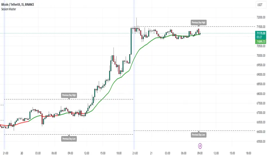
Volume Profile [Makit0]VOLUME PROFILE INDICATOR v0.5 beta
Volume Profile is suitable for day and swing trading on stock and futures markets, is a volume based indicator that gives you 6 key values for each session: POC, VAH, VAL, profile HIGH, LOW and MID levels. This project was born on the idea of plotting the RTH sessions Value Areas for /ES in an automated way, but you can select between 3 different sessions: RTH, GLOBEX and FULL sessions.
Some basic concepts:
- Volume Profile calculates the total volume for the session at each price level and give us market generated information about what price and range of prices are the most traded (where the value is)
- Value Area (VA): range of prices where 70% of the session volume is traded
- Value Area High (VAH): highest price within VA
- Value Area Low (VAL): lowest price within VA
- Point of Control (POC): the most traded price of the session (with the most volume)
- Session HIGH, LOW and MID levels are also important
There are a huge amount of things to know of Market Profile and Auction Theory like types of days, types of openings, relationships between value areas and openings... for those interested Jim Dalton's work is the way to come
I'm in my 2nd trading year and my goal for this year is learning to daytrade the futures markets thru the lens of Market Profile
For info on Volume Profile: TV Volume Profile wiki page at www.tradingview.com
For info on Market Profile and Market Auction Theory: Jim Dalton's book Mind over markets (this is a MUST)
BE AWARE: this indicator is based on the current chart's time interval and it only plots on 1, 2, 3, 5, 10, 15 and 30 minutes charts.
This is the correlation table TV uses in the Volume Profile Session Volume indicator (from the wiki above)
Chart Indicator
1 - 5 1
6 - 15 5
16 - 30 10
31 - 60 15
61 - 120 30
121 - 1D 60
This indicator doesn't follow that correlation, it doesn't get the volume data from a lower timeframe, it gets the data from the current chart resolution.
FEATURES
- 6 key values for each session: POC (solid yellow), VAH (solid red), VAL (solid green), profile HIGH (dashed silver), LOW (dashed silver) and MID (dotted silver) levels
- 3 sessions to choose for: RTH, GLOBEX and FULL
- select the numbers of sessions to plot by adding 12 hours periods back in time
- show/hide POC
- show/hide VAH & VAL
- show/hide session HIGH, LOW & MID levels
- highlight the periods of time out of the session (silver)
- extend the plotted lines all the way to the right, be careful this can turn the chart unreadable if there are a lot of sessions and lines plotted
SETTINGS
- Session: select between RTH (8:30 to 15:15 CT), GLOBEX (17:00 to 8:30 CT) and FULL (17:00 to 15:15 CT) sessions. RTH by default
- Last 12 hour periods to show: select the deph of the study by adding periods, for example, 60 periods are 30 natural days and around 22 trading days. 1 period by default
- Show POC (Point of Control): show/hide POC line. true by default
- Show VA (Value Area High & Low): show/hide VAH & VAL lines. true by default
- Show Range (Session High, Low & Mid): show/hide session HIGH, LOW & MID lines. true by default
- Highlight out of session: show/hide a silver shadow over the non session periods. true by default
- Extension: Extend all the plotted lines to the right. false by default
HOW TO SETUP
BE AWARE THIS INDICATOR PLOTS ONLY IN THE FOLLOWING CHART RESOLUTIONS: 1, 2, 3, 5, 10, 15 AND 30 MINUTES CHARTS. YOU MUST SELECT ONE OF THIS RESOLUTIONS TO THE INDICATOR BE ABLE TO PLOT
- By default this indicator plots all the levels for the last RTH session within the last 12 hours, if there is no plot try to adjust the 12 hours periods until the seesion and the periods match
- For Globex/Full sessions just select what you want from the dropdown menu and adjust the periods to plot the values
- Show or hide the levels you want with the 3 groups: POC line, VA lines and Session Range lines
- The highlight and extension options are for a better visibility of the levels as POC or VAH/VAL
THANKS TO
@watsonexchange for all the help, ideas and insights on this and the last two indicators (Market Delta & Market Internals) I'm working on my way to a 'clean chart' but for me it's not an easy path
@PineCoders for all the amazing stuff they do and all the help and tools they provide, in special the Script-Stopwatch at that was key in lowering this indicator's execution time
All the TV and Pine community, open source and shared knowledge are indeed the best way to help each other
IF YOU REALLY LIKE THIS WORK, please send me a comment or a private message and TELL ME WHAT you trade, HOW you trade it and your FAVOURITE SETUP for pulling out money from the market in a consistent basis, I'm learning to trade (this is my 2nd year) and I need all the help I can get
GOOD LUCK AND HAPPY TRADING

Multi-Timeframe SFP + SMTImportant: Please Read First
This indicator is not a "one size fits all" solution. It is a professional and complex tool that requires you to learn how to use it, in addition to backtesting different settings to discover what works best for your specific trading style and the assets you trade. The default settings provided are my personal preferences for trading higher-timeframe setups, but you are encouraged to experiment and find your own optimal configuration.
Please note that while this initial version is solid, it may still contain small errors or bugs. I will be actively working on improving the indicator over time. Also, be aware that the script is not written for maximum efficiency and may be resource-intensive, but this should not pose a problem for most users.
The source code for this indicator is open. If you truly want to understand precisely how all the logic works, you can copy and paste the code into an AI assistant like Gemini or ChatGPT and ask it to explain any part of the script to you.
Author's Preferred Settings (Guideline)
As a starting point, here are the settings I personally use for my trading:
SFP Timeframe: 4-Hour (Strength: 5-5)
Max Lookback: 35 Bars
Raid Expiration: 1 Bar
SFP Lines Limit: 1
SMT Timeframe 1: 30-Minute (Strength: 2-2) with 3-Minute LTF Detection.
SMT Timeframe 2: 15-Minute (Strength: 3-3) with 3-Minute LTF Detection.
SMT Timeframe 3: 1-Hour (Strength: 1-1) with 3-Minute LTF Detection.
SMT Timeframe 4: 15-Minute (Strength: 1-1) with 3-Minute LTF Detection.
Multi-Timeframe SMT: An Overview
This indicator is a powerful tool designed to identify high-probability trading setups by combining two key institutional concepts: Swing Failure Patterns (SFP) on a higher timeframe and Smart Money Technique (SMT) divergences on a lower timeframe. A key feature is the ability to configure and run up to four independent SMT analyses simultaneously, allowing you to monitor for divergences across multiple timeframes (e.g., 15m, 1H, 4H) from a single indicator.
Its primary purpose is to generate automated signals through TradingView's alert system. By setting up alerts, the script runs server-side, monitoring the market for you. When a setup presents itself, it will send a push notification to your device, allowing you to personally evaluate the trade without being tied to your screen.
The Strategy: HTF Liquidity Sweeps into LTF SMT
The core strategy is built on a classic institutional trading model:
Wait for a liquidity sweep on a significant high timeframe (e.g., 4-hour, Daily).
Once liquidity is taken, look for a confirmation of a shift in market structure on a lower timeframe.
This indicator uses an SMT divergence as that confirmation signal, indicating that smart money may be stepping in to reverse the price.
How It Works: The Two-Step Process
The indicator's logic follows a precise two-step process to generate a signal:
Step 1: The Swing Failure Pattern (SFP)
First, the indicator identifies a high-timeframe liquidity sweep. This is configured in the "Swing Failure Pattern (SFP) Timeframe" settings.
It looks for a candle that wicks above a previous high (or below a previous low) but then closes back within the range of that pivot. This action is known as a "raid" or a "swing failure," suggesting the move failed to find genuine momentum.
Step 2: The SMT Divergence
The moment a valid SFP is confirmed, the indicator's multiple SMT engines activate.
Each engine begins monitoring the specific SMT timeframe you have configured (e.g., "SMT Timeframe 1," "SMT Timeframe 2," etc.) for a Smart Money Technique (SMT) divergence.
An SMT divergence occurs when two closely correlated assets fail to move in sync. For example, after a raid on a high, Asset A makes a new high, but Asset B fails to do so. This disagreement suggests weakness and a potential reversal.
When the script finds this divergence, it plots the SMT line and triggers an alert.
The Power of Alerts
The true strength of this indicator lies in its alert capabilities. You can create alerts for both unconfirmed and confirmed SMTs.
Enable Alerts LTF Detection: These alerts trigger when an unconfirmed, potential SMT is spotted on the lower "LTF Detection" timeframe. While not yet confirmed, these early alerts can notify you of a potential move before it fully happens, allowing you to be ahead of the curve and find the best possible trade entries.
Enable Alerts Confirmed SMT: These alerts trigger only when a permanent, confirmed SMT line is plotted on your chosen SMT timeframe. These signals are more reliable but occur later than the early detection alerts.
Key Concepts Explained
What is Pivot Strength?
Pivot Strength determines how significant a high or low needs to be to qualify as a valid structural point. A setting of 5-5, for example, means that for a candle's high to be considered a valid pivot high, its high must be higher than the highs of the 5 candles to its left and the 5 candles to its right.
Higher Strength (e.g., 5-5, 8-8): Creates fewer, but more significant, pivots. This is ideal for identifying major structural highs and lows on higher timeframes.
Lower Strength (e.g., 2-2, 3-3): Creates more pivots, making it suitable for identifying the smaller shifts in momentum on lower timeframes.
Raid Expiration & Validity
An SFP signal is not valid forever. The "Raid Expiration" setting determines how many SFP timeframe bars can pass after a raid before that signal is considered "stale" and can no longer be used to validate an SMT. This ensures your SMT divergences are always in response to recent liquidity sweeps.
Why You Must Be on the Right Chart Timeframe to See SMT Lines
Pine Script™ has a fundamental rule: an indicator running on a chart can only "see" the bars of that chart's timeframe or higher.
When the SMT logic is set to the 15-minute timeframe, it calculates its pivots based on 15-minute data. To accurately plot lines connecting these pivots, you must be on a 15-minute chart or lower (e.g., 5-minute, 1-minute).
If you are on a higher timeframe chart, like the 1-hour, the 15-minute bars do not exist on that chart, so the indicator has no bars to draw the lines on.
This is precisely why the alert system is so powerful. You can set your alert to run on the 15-minute timeframe, and TradingView's servers will monitor that timeframe for you, sending a notification regardless of what chart you are currently viewing.
LANZ Strategy 3.0 [Backtest]🔷 LANZ Strategy 3.0 — Asian Range Fibonacci Scalping Strategy
LANZ Strategy 3.0 is a precision-engineered backtesting tool tailored for intraday traders who rely on the Asian session range to determine directional bias. This strategy implements dynamic Fibonacci projections and strict time-window validation to simulate a clean and disciplined trading environment.
🧠 Core Components:
Asian Range Bias Definition: Direction is established between 01:15–02:15 a.m. NY time based on the candle’s close in relation to the midpoint of the Asian session range (18:00–01:15 NY).
Limit Order Execution: Only one trade is placed daily, using a limit order at the Asian range high (for sells) or low (for buys), between 01:15–08:00 a.m. NY.
Fibonacci-Based TP/SL:
Original Mode: TP = 2.25x range, SL = 0.75x range.
Optimized Mode: TP = 1.95x range, SL = 0.65x range.
No Trade After 08:00 NY: If the limit order is not executed before 08:00 a.m. NY, it is canceled.
Fallback Logic at 02:15 NY: If the market direction misaligns with the setup at 02:15 a.m., the system re-evaluates and can re-issue the order.
End-of-Day Closure: All positions are closed at 15:45 NY if still open.
📊 Backtest-Ready Design:
Entries and exits are executed using strategy.entry() and strategy.exit() functions.
Position size is fixed via capital risk allocation ($100 per trade by default).
Only one position can be active at a time, ensuring controlled risk.
📝 Notes:
This strategy is ideal for assets sensitive to the Asian/London session overlap, such as Forex pairs and indices.
Easily switch between Fibonacci versions using a single dropdown input.
Fully deterministic: all entries are based on pre-defined conditions and time constraints.
👤 Credits:
Strategy developed by rau_u_lanz using Pine Script v6. Built for traders who favor clean sessions, directional clarity, and consistent execution using time-based logic and Fibonacci projections.

Daily High/Low (15m) + EMA Pre-Market H/L + ORBStraightforward:
I built a swing-trading indicator with ChatGPT that plots 15-minute highs and lows, draws pre-market high/low lines, and adds a 15-minute opening-range breakout feature.
Technical:
Using ChatGPT, I developed a swing-trade indicator that calculates 15-minute highs/lows, overlays pre-market high and low levels, and includes a 15-minute Opening Range Breakout (ORB) module.
Promotional:
I created a ChatGPT-powered swing-trading indicator that maps 15-minute highs/lows, marks pre-market levels, and features a 15-minute Opening Range Breakout for clearer entries.

Markov Chain [3D] | FractalystWhat exactly is a Markov Chain?
This indicator uses a Markov Chain model to analyze, quantify, and visualize the transitions between market regimes (Bull, Bear, Neutral) on your chart. It dynamically detects these regimes in real-time, calculates transition probabilities, and displays them as animated 3D spheres and arrows, giving traders intuitive insight into current and future market conditions.
How does a Markov Chain work, and how should I read this spheres-and-arrows diagram?
Think of three weather modes: Sunny, Rainy, Cloudy.
Each sphere is one mode. The loop on a sphere means “stay the same next step” (e.g., Sunny again tomorrow).
The arrows leaving a sphere show where things usually go next if they change (e.g., Sunny moving to Cloudy).
Some paths matter more than others. A more prominent loop means the current mode tends to persist. A more prominent outgoing arrow means a change to that destination is the usual next step.
Direction isn’t symmetric: moving Sunny→Cloudy can behave differently than Cloudy→Sunny.
Now relabel the spheres to markets: Bull, Bear, Neutral.
Spheres: market regimes (uptrend, downtrend, range).
Self‑loop: tendency for the current regime to continue on the next bar.
Arrows: the most common next regime if a switch happens.
How to read: Start at the sphere that matches current bar state. If the loop stands out, expect continuation. If one outgoing path stands out, that switch is the typical next step. Opposite directions can differ (Bear→Neutral doesn’t have to match Neutral→Bear).
What states and transitions are shown?
The three market states visualized are:
Bullish (Bull): Upward or strong-market regime.
Bearish (Bear): Downward or weak-market regime.
Neutral: Sideways or range-bound regime.
Bidirectional animated arrows and probability labels show how likely the market is to move from one regime to another (e.g., Bull → Bear or Neutral → Bull).
How does the regime detection system work?
You can use either built-in price returns (based on adaptive Z-score normalization) or supply three custom indicators (such as volume, oscillators, etc.).
Values are statistically normalized (Z-scored) over a configurable lookback period.
The normalized outputs are classified into Bull, Bear, or Neutral zones.
If using three indicators, their regime signals are averaged and smoothed for robustness.
How are transition probabilities calculated?
On every confirmed bar, the algorithm tracks the sequence of detected market states, then builds a rolling window of transitions.
The code maintains a transition count matrix for all regime pairs (e.g., Bull → Bear).
Transition probabilities are extracted for each possible state change using Laplace smoothing for numerical stability, and frequently updated in real-time.
What is unique about the visualization?
3D animated spheres represent each regime and change visually when active.
Animated, bidirectional arrows reveal transition probabilities and allow you to see both dominant and less likely regime flows.
Particles (moving dots) animate along the arrows, enhancing the perception of regime flow direction and speed.
All elements dynamically update with each new price bar, providing a live market map in an intuitive, engaging format.
Can I use custom indicators for regime classification?
Yes! Enable the "Custom Indicators" switch and select any three chart series as inputs. These will be normalized and combined (each with equal weight), broadening the regime classification beyond just price-based movement.
What does the “Lookback Period” control?
Lookback Period (default: 100) sets how much historical data builds the probability matrix. Shorter periods adapt faster to regime changes but may be noisier. Longer periods are more stable but slower to adapt.
How is this different from a Hidden Markov Model (HMM)?
It sets the window for both regime detection and probability calculations. Lower values make the system more reactive, but potentially noisier. Higher values smooth estimates and make the system more robust.
How is this Markov Chain different from a Hidden Markov Model (HMM)?
Markov Chain (as here): All market regimes (Bull, Bear, Neutral) are directly observable on the chart. The transition matrix is built from actual detected regimes, keeping the model simple and interpretable.
Hidden Markov Model: The actual regimes are unobservable ("hidden") and must be inferred from market output or indicator "emissions" using statistical learning algorithms. HMMs are more complex, can capture more subtle structure, but are harder to visualize and require additional machine learning steps for training.
A standard Markov Chain models transitions between observable states using a simple transition matrix, while a Hidden Markov Model assumes the true states are hidden (latent) and must be inferred from observable “emissions” like price or volume data. In practical terms, a Markov Chain is transparent and easier to implement and interpret; an HMM is more expressive but requires statistical inference to estimate hidden states from data.
Markov Chain: states are observable; you directly count or estimate transition probabilities between visible states. This makes it simpler, faster, and easier to validate and tune.
HMM: states are hidden; you only observe emissions generated by those latent states. Learning involves machine learning/statistical algorithms (commonly Baum–Welch/EM for training and Viterbi for decoding) to infer both the transition dynamics and the most likely hidden state sequence from data.
How does the indicator avoid “repainting” or look-ahead bias?
All regime changes and matrix updates happen only on confirmed (closed) bars, so no future data is leaked, ensuring reliable real-time operation.
Are there practical tuning tips?
Tune the Lookback Period for your asset/timeframe: shorter for fast markets, longer for stability.
Use custom indicators if your asset has unique regime drivers.
Watch for rapid changes in transition probabilities as early warning of a possible regime shift.
Who is this indicator for?
Quants and quantitative researchers exploring probabilistic market modeling, especially those interested in regime-switching dynamics and Markov models.
Programmers and system developers who need a probabilistic regime filter for systematic and algorithmic backtesting:
The Markov Chain indicator is ideally suited for programmatic integration via its bias output (1 = Bull, 0 = Neutral, -1 = Bear).
Although the visualization is engaging, the core output is designed for automated, rules-based workflows—not for discretionary/manual trading decisions.
Developers can connect the indicator’s output directly to their Pine Script logic (using input.source()), allowing rapid and robust backtesting of regime-based strategies.
It acts as a plug-and-play regime filter: simply plug the bias output into your entry/exit logic, and you have a scientifically robust, probabilistically-derived signal for filtering, timing, position sizing, or risk regimes.
The MC's output is intentionally "trinary" (1/0/-1), focusing on clear regime states for unambiguous decision-making in code. If you require nuanced, multi-probability or soft-label state vectors, consider expanding the indicator or stacking it with a probability-weighted logic layer in your scripting.
Because it avoids subjectivity, this approach is optimal for systematic quants, algo developers building backtested, repeatable strategies based on probabilistic regime analysis.
What's the mathematical foundation behind this?
The mathematical foundation behind this Markov Chain indicator—and probabilistic regime detection in finance—draws from two principal models: the (standard) Markov Chain and the Hidden Markov Model (HMM).
How to use this indicator programmatically?
The Markov Chain indicator automatically exports a bias value (+1 for Bullish, -1 for Bearish, 0 for Neutral) as a plot visible in the Data Window. This allows you to integrate its regime signal into your own scripts and strategies for backtesting, automation, or live trading.
Step-by-Step Integration with Pine Script (input.source)
Add the Markov Chain indicator to your chart.
This must be done first, since your custom script will "pull" the bias signal from the indicator's plot.
In your strategy, create an input using input.source()
Example:
//@version=5
strategy("MC Bias Strategy Example")
mcBias = input.source(close, "MC Bias Source")
After saving, go to your script’s settings. For the “MC Bias Source” input, select the plot/output of the Markov Chain indicator (typically its bias plot).
Use the bias in your trading logic
Example (long only on Bull, flat otherwise):
if mcBias == 1
strategy.entry("Long", strategy.long)
else
strategy.close("Long")
For more advanced workflows, combine mcBias with additional filters or trailing stops.
How does this work behind-the-scenes?
TradingView’s input.source() lets you use any plot from another indicator as a real-time, “live” data feed in your own script (source).
The selected bias signal is available to your Pine code as a variable, enabling logical decisions based on regime (trend-following, mean-reversion, etc.).
This enables powerful strategy modularity : decouple regime detection from entry/exit logic, allowing fast experimentation without rewriting core signal code.
Integrating 45+ Indicators with Your Markov Chain — How & Why
The Enhanced Custom Indicators Export script exports a massive suite of over 45 technical indicators—ranging from classic momentum (RSI, MACD, Stochastic, etc.) to trend, volume, volatility, and oscillator tools—all pre-calculated, centered/scaled, and available as plots.
// Enhanced Custom Indicators Export - 45 Technical Indicators
// Comprehensive technical analysis suite for advanced market regime detection
//@version=6
indicator('Enhanced Custom Indicators Export | Fractalyst', shorttitle='Enhanced CI Export', overlay=false, scale=scale.right, max_labels_count=500, max_lines_count=500)
// |----- Input Parameters -----| //
momentum_group = "Momentum Indicators"
trend_group = "Trend Indicators"
volume_group = "Volume Indicators"
volatility_group = "Volatility Indicators"
oscillator_group = "Oscillator Indicators"
display_group = "Display Settings"
// Common lengths
length_14 = input.int(14, "Standard Length (14)", minval=1, maxval=100, group=momentum_group)
length_20 = input.int(20, "Medium Length (20)", minval=1, maxval=200, group=trend_group)
length_50 = input.int(50, "Long Length (50)", minval=1, maxval=200, group=trend_group)
// Display options
show_table = input.bool(true, "Show Values Table", group=display_group)
table_size = input.string("Small", "Table Size", options= , group=display_group)
// |----- MOMENTUM INDICATORS (15 indicators) -----| //
// 1. RSI (Relative Strength Index)
rsi_14 = ta.rsi(close, length_14)
rsi_centered = rsi_14 - 50
// 2. Stochastic Oscillator
stoch_k = ta.stoch(close, high, low, length_14)
stoch_d = ta.sma(stoch_k, 3)
stoch_centered = stoch_k - 50
// 3. Williams %R
williams_r = ta.stoch(close, high, low, length_14) - 100
// 4. MACD (Moving Average Convergence Divergence)
= ta.macd(close, 12, 26, 9)
// 5. Momentum (Rate of Change)
momentum = ta.mom(close, length_14)
momentum_pct = (momentum / close ) * 100
// 6. Rate of Change (ROC)
roc = ta.roc(close, length_14)
// 7. Commodity Channel Index (CCI)
cci = ta.cci(close, length_20)
// 8. Money Flow Index (MFI)
mfi = ta.mfi(close, length_14)
mfi_centered = mfi - 50
// 9. Awesome Oscillator (AO)
ao = ta.sma(hl2, 5) - ta.sma(hl2, 34)
// 10. Accelerator Oscillator (AC)
ac = ao - ta.sma(ao, 5)
// 11. Chande Momentum Oscillator (CMO)
cmo = ta.cmo(close, length_14)
// 12. Detrended Price Oscillator (DPO)
dpo = close - ta.sma(close, length_20)
// 13. Price Oscillator (PPO)
ppo = ta.sma(close, 12) - ta.sma(close, 26)
ppo_pct = (ppo / ta.sma(close, 26)) * 100
// 14. TRIX
trix_ema1 = ta.ema(close, length_14)
trix_ema2 = ta.ema(trix_ema1, length_14)
trix_ema3 = ta.ema(trix_ema2, length_14)
trix = ta.roc(trix_ema3, 1) * 10000
// 15. Klinger Oscillator
klinger = ta.ema(volume * (high + low + close) / 3, 34) - ta.ema(volume * (high + low + close) / 3, 55)
// 16. Fisher Transform
fisher_hl2 = 0.5 * (hl2 - ta.lowest(hl2, 10)) / (ta.highest(hl2, 10) - ta.lowest(hl2, 10)) - 0.25
fisher = 0.5 * math.log((1 + fisher_hl2) / (1 - fisher_hl2))
// 17. Stochastic RSI
stoch_rsi = ta.stoch(rsi_14, rsi_14, rsi_14, length_14)
stoch_rsi_centered = stoch_rsi - 50
// 18. Relative Vigor Index (RVI)
rvi_num = ta.swma(close - open)
rvi_den = ta.swma(high - low)
rvi = rvi_den != 0 ? rvi_num / rvi_den : 0
// 19. Balance of Power (BOP)
bop = (close - open) / (high - low)
// |----- TREND INDICATORS (10 indicators) -----| //
// 20. Simple Moving Average Momentum
sma_20 = ta.sma(close, length_20)
sma_momentum = ((close - sma_20) / sma_20) * 100
// 21. Exponential Moving Average Momentum
ema_20 = ta.ema(close, length_20)
ema_momentum = ((close - ema_20) / ema_20) * 100
// 22. Parabolic SAR
sar = ta.sar(0.02, 0.02, 0.2)
sar_trend = close > sar ? 1 : -1
// 23. Linear Regression Slope
lr_slope = ta.linreg(close, length_20, 0) - ta.linreg(close, length_20, 1)
// 24. Moving Average Convergence (MAC)
mac = ta.sma(close, 10) - ta.sma(close, 30)
// 25. Trend Intensity Index (TII)
tii_sum = 0.0
for i = 1 to length_20
tii_sum += close > close ? 1 : 0
tii = (tii_sum / length_20) * 100
// 26. Ichimoku Cloud Components
ichimoku_tenkan = (ta.highest(high, 9) + ta.lowest(low, 9)) / 2
ichimoku_kijun = (ta.highest(high, 26) + ta.lowest(low, 26)) / 2
ichimoku_signal = ichimoku_tenkan > ichimoku_kijun ? 1 : -1
// 27. MESA Adaptive Moving Average (MAMA)
mama_alpha = 2.0 / (length_20 + 1)
mama = ta.ema(close, length_20)
mama_momentum = ((close - mama) / mama) * 100
// 28. Zero Lag Exponential Moving Average (ZLEMA)
zlema_lag = math.round((length_20 - 1) / 2)
zlema_data = close + (close - close )
zlema = ta.ema(zlema_data, length_20)
zlema_momentum = ((close - zlema) / zlema) * 100
// |----- VOLUME INDICATORS (6 indicators) -----| //
// 29. On-Balance Volume (OBV)
obv = ta.obv
// 30. Volume Rate of Change (VROC)
vroc = ta.roc(volume, length_14)
// 31. Price Volume Trend (PVT)
pvt = ta.pvt
// 32. Negative Volume Index (NVI)
nvi = 0.0
nvi := volume < volume ? nvi + ((close - close ) / close ) * nvi : nvi
// 33. Positive Volume Index (PVI)
pvi = 0.0
pvi := volume > volume ? pvi + ((close - close ) / close ) * pvi : pvi
// 34. Volume Oscillator
vol_osc = ta.sma(volume, 5) - ta.sma(volume, 10)
// 35. Ease of Movement (EOM)
eom_distance = high - low
eom_box_height = volume / 1000000
eom = eom_box_height != 0 ? eom_distance / eom_box_height : 0
eom_sma = ta.sma(eom, length_14)
// 36. Force Index
force_index = volume * (close - close )
force_index_sma = ta.sma(force_index, length_14)
// |----- VOLATILITY INDICATORS (10 indicators) -----| //
// 37. Average True Range (ATR)
atr = ta.atr(length_14)
atr_pct = (atr / close) * 100
// 38. Bollinger Bands Position
bb_basis = ta.sma(close, length_20)
bb_dev = 2.0 * ta.stdev(close, length_20)
bb_upper = bb_basis + bb_dev
bb_lower = bb_basis - bb_dev
bb_position = bb_dev != 0 ? (close - bb_basis) / bb_dev : 0
bb_width = bb_dev != 0 ? (bb_upper - bb_lower) / bb_basis * 100 : 0
// 39. Keltner Channels Position
kc_basis = ta.ema(close, length_20)
kc_range = ta.ema(ta.tr, length_20)
kc_upper = kc_basis + (2.0 * kc_range)
kc_lower = kc_basis - (2.0 * kc_range)
kc_position = kc_range != 0 ? (close - kc_basis) / kc_range : 0
// 40. Donchian Channels Position
dc_upper = ta.highest(high, length_20)
dc_lower = ta.lowest(low, length_20)
dc_basis = (dc_upper + dc_lower) / 2
dc_position = (dc_upper - dc_lower) != 0 ? (close - dc_basis) / (dc_upper - dc_lower) : 0
// 41. Standard Deviation
std_dev = ta.stdev(close, length_20)
std_dev_pct = (std_dev / close) * 100
// 42. Relative Volatility Index (RVI)
rvi_up = ta.stdev(close > close ? close : 0, length_14)
rvi_down = ta.stdev(close < close ? close : 0, length_14)
rvi_total = rvi_up + rvi_down
rvi_volatility = rvi_total != 0 ? (rvi_up / rvi_total) * 100 : 50
// 43. Historical Volatility
hv_returns = math.log(close / close )
hv = ta.stdev(hv_returns, length_20) * math.sqrt(252) * 100
// 44. Garman-Klass Volatility
gk_vol = math.log(high/low) * math.log(high/low) - (2*math.log(2)-1) * math.log(close/open) * math.log(close/open)
gk_volatility = math.sqrt(ta.sma(gk_vol, length_20)) * 100
// 45. Parkinson Volatility
park_vol = math.log(high/low) * math.log(high/low)
parkinson = math.sqrt(ta.sma(park_vol, length_20) / (4 * math.log(2))) * 100
// 46. Rogers-Satchell Volatility
rs_vol = math.log(high/close) * math.log(high/open) + math.log(low/close) * math.log(low/open)
rogers_satchell = math.sqrt(ta.sma(rs_vol, length_20)) * 100
// |----- OSCILLATOR INDICATORS (5 indicators) -----| //
// 47. Elder Ray Index
elder_bull = high - ta.ema(close, 13)
elder_bear = low - ta.ema(close, 13)
elder_power = elder_bull + elder_bear
// 48. Schaff Trend Cycle (STC)
stc_macd = ta.ema(close, 23) - ta.ema(close, 50)
stc_k = ta.stoch(stc_macd, stc_macd, stc_macd, 10)
stc_d = ta.ema(stc_k, 3)
stc = ta.stoch(stc_d, stc_d, stc_d, 10)
// 49. Coppock Curve
coppock_roc1 = ta.roc(close, 14)
coppock_roc2 = ta.roc(close, 11)
coppock = ta.wma(coppock_roc1 + coppock_roc2, 10)
// 50. Know Sure Thing (KST)
kst_roc1 = ta.roc(close, 10)
kst_roc2 = ta.roc(close, 15)
kst_roc3 = ta.roc(close, 20)
kst_roc4 = ta.roc(close, 30)
kst = ta.sma(kst_roc1, 10) + 2*ta.sma(kst_roc2, 10) + 3*ta.sma(kst_roc3, 10) + 4*ta.sma(kst_roc4, 15)
// 51. Percentage Price Oscillator (PPO)
ppo_line = ((ta.ema(close, 12) - ta.ema(close, 26)) / ta.ema(close, 26)) * 100
ppo_signal = ta.ema(ppo_line, 9)
ppo_histogram = ppo_line - ppo_signal
// |----- PLOT MAIN INDICATORS -----| //
// Plot key momentum indicators
plot(rsi_centered, title="01_RSI_Centered", color=color.purple, linewidth=1)
plot(stoch_centered, title="02_Stoch_Centered", color=color.blue, linewidth=1)
plot(williams_r, title="03_Williams_R", color=color.red, linewidth=1)
plot(macd_histogram, title="04_MACD_Histogram", color=color.orange, linewidth=1)
plot(cci, title="05_CCI", color=color.green, linewidth=1)
// Plot trend indicators
plot(sma_momentum, title="06_SMA_Momentum", color=color.navy, linewidth=1)
plot(ema_momentum, title="07_EMA_Momentum", color=color.maroon, linewidth=1)
plot(sar_trend, title="08_SAR_Trend", color=color.teal, linewidth=1)
plot(lr_slope, title="09_LR_Slope", color=color.lime, linewidth=1)
plot(mac, title="10_MAC", color=color.fuchsia, linewidth=1)
// Plot volatility indicators
plot(atr_pct, title="11_ATR_Pct", color=color.yellow, linewidth=1)
plot(bb_position, title="12_BB_Position", color=color.aqua, linewidth=1)
plot(kc_position, title="13_KC_Position", color=color.olive, linewidth=1)
plot(std_dev_pct, title="14_StdDev_Pct", color=color.silver, linewidth=1)
plot(bb_width, title="15_BB_Width", color=color.gray, linewidth=1)
// Plot volume indicators
plot(vroc, title="16_VROC", color=color.blue, linewidth=1)
plot(eom_sma, title="17_EOM", color=color.red, linewidth=1)
plot(vol_osc, title="18_Vol_Osc", color=color.green, linewidth=1)
plot(force_index_sma, title="19_Force_Index", color=color.orange, linewidth=1)
plot(obv, title="20_OBV", color=color.purple, linewidth=1)
// Plot additional oscillators
plot(ao, title="21_Awesome_Osc", color=color.navy, linewidth=1)
plot(cmo, title="22_CMO", color=color.maroon, linewidth=1)
plot(dpo, title="23_DPO", color=color.teal, linewidth=1)
plot(trix, title="24_TRIX", color=color.lime, linewidth=1)
plot(fisher, title="25_Fisher", color=color.fuchsia, linewidth=1)
// Plot more momentum indicators
plot(mfi_centered, title="26_MFI_Centered", color=color.yellow, linewidth=1)
plot(ac, title="27_AC", color=color.aqua, linewidth=1)
plot(ppo_pct, title="28_PPO_Pct", color=color.olive, linewidth=1)
plot(stoch_rsi_centered, title="29_StochRSI_Centered", color=color.silver, linewidth=1)
plot(klinger, title="30_Klinger", color=color.gray, linewidth=1)
// Plot trend continuation
plot(tii, title="31_TII", color=color.blue, linewidth=1)
plot(ichimoku_signal, title="32_Ichimoku_Signal", color=color.red, linewidth=1)
plot(mama_momentum, title="33_MAMA_Momentum", color=color.green, linewidth=1)
plot(zlema_momentum, title="34_ZLEMA_Momentum", color=color.orange, linewidth=1)
plot(bop, title="35_BOP", color=color.purple, linewidth=1)
// Plot volume continuation
plot(nvi, title="36_NVI", color=color.navy, linewidth=1)
plot(pvi, title="37_PVI", color=color.maroon, linewidth=1)
plot(momentum_pct, title="38_Momentum_Pct", color=color.teal, linewidth=1)
plot(roc, title="39_ROC", color=color.lime, linewidth=1)
plot(rvi, title="40_RVI", color=color.fuchsia, linewidth=1)
// Plot volatility continuation
plot(dc_position, title="41_DC_Position", color=color.yellow, linewidth=1)
plot(rvi_volatility, title="42_RVI_Volatility", color=color.aqua, linewidth=1)
plot(hv, title="43_Historical_Vol", color=color.olive, linewidth=1)
plot(gk_volatility, title="44_GK_Volatility", color=color.silver, linewidth=1)
plot(parkinson, title="45_Parkinson_Vol", color=color.gray, linewidth=1)
// Plot final oscillators
plot(rogers_satchell, title="46_RS_Volatility", color=color.blue, linewidth=1)
plot(elder_power, title="47_Elder_Power", color=color.red, linewidth=1)
plot(stc, title="48_STC", color=color.green, linewidth=1)
plot(coppock, title="49_Coppock", color=color.orange, linewidth=1)
plot(kst, title="50_KST", color=color.purple, linewidth=1)
// Plot final indicators
plot(ppo_histogram, title="51_PPO_Histogram", color=color.navy, linewidth=1)
plot(pvt, title="52_PVT", color=color.maroon, linewidth=1)
// |----- Reference Lines -----| //
hline(0, "Zero Line", color=color.gray, linestyle=hline.style_dashed, linewidth=1)
hline(50, "Midline", color=color.gray, linestyle=hline.style_dotted, linewidth=1)
hline(-50, "Lower Midline", color=color.gray, linestyle=hline.style_dotted, linewidth=1)
hline(25, "Upper Threshold", color=color.gray, linestyle=hline.style_dotted, linewidth=1)
hline(-25, "Lower Threshold", color=color.gray, linestyle=hline.style_dotted, linewidth=1)
// |----- Enhanced Information Table -----| //
if show_table and barstate.islast
table_position = position.top_right
table_text_size = table_size == "Tiny" ? size.tiny : table_size == "Small" ? size.small : size.normal
var table info_table = table.new(table_position, 3, 18, bgcolor=color.new(color.white, 85), border_width=1, border_color=color.gray)
// Headers
table.cell(info_table, 0, 0, 'Category', text_color=color.black, text_size=table_text_size, bgcolor=color.new(color.blue, 70))
table.cell(info_table, 1, 0, 'Indicator', text_color=color.black, text_size=table_text_size, bgcolor=color.new(color.blue, 70))
table.cell(info_table, 2, 0, 'Value', text_color=color.black, text_size=table_text_size, bgcolor=color.new(color.blue, 70))
// Key Momentum Indicators
table.cell(info_table, 0, 1, 'MOMENTUM', text_color=color.purple, text_size=table_text_size, bgcolor=color.new(color.purple, 90))
table.cell(info_table, 1, 1, 'RSI Centered', text_color=color.purple, text_size=table_text_size)
table.cell(info_table, 2, 1, str.tostring(rsi_centered, '0.00'), text_color=color.purple, text_size=table_text_size)
table.cell(info_table, 0, 2, '', text_color=color.blue, text_size=table_text_size)
table.cell(info_table, 1, 2, 'Stoch Centered', text_color=color.blue, text_size=table_text_size)
table.cell(info_table, 2, 2, str.tostring(stoch_centered, '0.00'), text_color=color.blue, text_size=table_text_size)
table.cell(info_table, 0, 3, '', text_color=color.red, text_size=table_text_size)
table.cell(info_table, 1, 3, 'Williams %R', text_color=color.red, text_size=table_text_size)
table.cell(info_table, 2, 3, str.tostring(williams_r, '0.00'), text_color=color.red, text_size=table_text_size)
table.cell(info_table, 0, 4, '', text_color=color.orange, text_size=table_text_size)
table.cell(info_table, 1, 4, 'MACD Histogram', text_color=color.orange, text_size=table_text_size)
table.cell(info_table, 2, 4, str.tostring(macd_histogram, '0.000'), text_color=color.orange, text_size=table_text_size)
table.cell(info_table, 0, 5, '', text_color=color.green, text_size=table_text_size)
table.cell(info_table, 1, 5, 'CCI', text_color=color.green, text_size=table_text_size)
table.cell(info_table, 2, 5, str.tostring(cci, '0.00'), text_color=color.green, text_size=table_text_size)
// Key Trend Indicators
table.cell(info_table, 0, 6, 'TREND', text_color=color.navy, text_size=table_text_size, bgcolor=color.new(color.navy, 90))
table.cell(info_table, 1, 6, 'SMA Momentum %', text_color=color.navy, text_size=table_text_size)
table.cell(info_table, 2, 6, str.tostring(sma_momentum, '0.00'), text_color=color.navy, text_size=table_text_size)
table.cell(info_table, 0, 7, '', text_color=color.maroon, text_size=table_text_size)
table.cell(info_table, 1, 7, 'EMA Momentum %', text_color=color.maroon, text_size=table_text_size)
table.cell(info_table, 2, 7, str.tostring(ema_momentum, '0.00'), text_color=color.maroon, text_size=table_text_size)
table.cell(info_table, 0, 8, '', text_color=color.teal, text_size=table_text_size)
table.cell(info_table, 1, 8, 'SAR Trend', text_color=color.teal, text_size=table_text_size)
table.cell(info_table, 2, 8, str.tostring(sar_trend, '0'), text_color=color.teal, text_size=table_text_size)
table.cell(info_table, 0, 9, '', text_color=color.lime, text_size=table_text_size)
table.cell(info_table, 1, 9, 'Linear Regression', text_color=color.lime, text_size=table_text_size)
table.cell(info_table, 2, 9, str.tostring(lr_slope, '0.000'), text_color=color.lime, text_size=table_text_size)
// Key Volatility Indicators
table.cell(info_table, 0, 10, 'VOLATILITY', text_color=color.yellow, text_size=table_text_size, bgcolor=color.new(color.yellow, 90))
table.cell(info_table, 1, 10, 'ATR %', text_color=color.yellow, text_size=table_text_size)
table.cell(info_table, 2, 10, str.tostring(atr_pct, '0.00'), text_color=color.yellow, text_size=table_text_size)
table.cell(info_table, 0, 11, '', text_color=color.aqua, text_size=table_text_size)
table.cell(info_table, 1, 11, 'BB Position', text_color=color.aqua, text_size=table_text_size)
table.cell(info_table, 2, 11, str.tostring(bb_position, '0.00'), text_color=color.aqua, text_size=table_text_size)
table.cell(info_table, 0, 12, '', text_color=color.olive, text_size=table_text_size)
table.cell(info_table, 1, 12, 'KC Position', text_color=color.olive, text_size=table_text_size)
table.cell(info_table, 2, 12, str.tostring(kc_position, '0.00'), text_color=color.olive, text_size=table_text_size)
// Key Volume Indicators
table.cell(info_table, 0, 13, 'VOLUME', text_color=color.blue, text_size=table_text_size, bgcolor=color.new(color.blue, 90))
table.cell(info_table, 1, 13, 'Volume ROC', text_color=color.blue, text_size=table_text_size)
table.cell(info_table, 2, 13, str.tostring(vroc, '0.00'), text_color=color.blue, text_size=table_text_size)
table.cell(info_table, 0, 14, '', text_color=color.red, text_size=table_text_size)
table.cell(info_table, 1, 14, 'EOM', text_color=color.red, text_size=table_text_size)
table.cell(info_table, 2, 14, str.tostring(eom_sma, '0.000'), text_color=color.red, text_size=table_text_size)
// Key Oscillators
table.cell(info_table, 0, 15, 'OSCILLATORS', text_color=color.purple, text_size=table_text_size, bgcolor=color.new(color.purple, 90))
table.cell(info_table, 1, 15, 'Awesome Osc', text_color=color.blue, text_size=table_text_size)
table.cell(info_table, 2, 15, str.tostring(ao, '0.000'), text_color=color.blue, text_size=table_text_size)
table.cell(info_table, 0, 16, '', text_color=color.red, text_size=table_text_size)
table.cell(info_table, 1, 16, 'Fisher Transform', text_color=color.red, text_size=table_text_size)
table.cell(info_table, 2, 16, str.tostring(fisher, '0.000'), text_color=color.red, text_size=table_text_size)
// Summary Statistics
table.cell(info_table, 0, 17, 'SUMMARY', text_color=color.black, text_size=table_text_size, bgcolor=color.new(color.gray, 70))
table.cell(info_table, 1, 17, 'Total Indicators: 52', text_color=color.black, text_size=table_text_size)
regime_color = rsi_centered > 10 ? color.green : rsi_centered < -10 ? color.red : color.gray
regime_text = rsi_centered > 10 ? "BULLISH" : rsi_centered < -10 ? "BEARISH" : "NEUTRAL"
table.cell(info_table, 2, 17, regime_text, text_color=regime_color, text_size=table_text_size)
This makes it the perfect “indicator backbone” for quantitative and systematic traders who want to prototype, combine, and test new regime detection models—especially in combination with the Markov Chain indicator.
How to use this script with the Markov Chain for research and backtesting:
Add the Enhanced Indicator Export to your chart.
Every calculated indicator is available as an individual data stream.
Connect the indicator(s) you want as custom input(s) to the Markov Chain’s “Custom Indicators” option.
In the Markov Chain indicator’s settings, turn ON the custom indicator mode.
For each of the three custom indicator inputs, select the exported plot from the Enhanced Export script—the menu lists all 45+ signals by name.
This creates a powerful, modular regime-detection engine where you can mix-and-match momentum, trend, volume, or custom combinations for advanced filtering.
Backtest regime logic directly.
Once you’ve connected your chosen indicators, the Markov Chain script performs regime detection (Bull/Neutral/Bear) based on your selected features—not just price returns.
The regime detection is robust, automatically normalized (using Z-score), and outputs bias (1, -1, 0) for plug-and-play integration.
Export the regime bias for programmatic use.
As described above, use input.source() in your Pine Script strategy or system and link the bias output.
You can now filter signals, control trade direction/size, or design pairs-trading that respect true, indicator-driven market regimes.
With this framework, you’re not limited to static or simplistic regime filters. You can rigorously define, test, and refine what “market regime” means for your strategies—using the technical features that matter most to you.
Optimize your signal generation by backtesting across a universe of meaningful indicator blends.
Enhance risk management with objective, real-time regime boundaries.
Accelerate your research: iterate quickly, swap indicator components, and see results with minimal code changes.
Automate multi-asset or pairs-trading by integrating regime context directly into strategy logic.
Add both scripts to your chart, connect your preferred features, and start investigating your best regime-based trades—entirely within the TradingView ecosystem.
References & Further Reading
Ang, A., & Bekaert, G. (2002). “Regime Switches in Interest Rates.” Journal of Business & Economic Statistics, 20(2), 163–182.
Hamilton, J. D. (1989). “A New Approach to the Economic Analysis of Nonstationary Time Series and the Business Cycle.” Econometrica, 57(2), 357–384.
Markov, A. A. (1906). "Extension of the Limit Theorems of Probability Theory to a Sum of Variables Connected in a Chain." The Notes of the Imperial Academy of Sciences of St. Petersburg.
Guidolin, M., & Timmermann, A. (2007). “Asset Allocation under Multivariate Regime Switching.” Journal of Economic Dynamics and Control, 31(11), 3503–3544.
Murphy, J. J. (1999). Technical Analysis of the Financial Markets. New York Institute of Finance.
Brock, W., Lakonishok, J., & LeBaron, B. (1992). “Simple Technical Trading Rules and the Stochastic Properties of Stock Returns.” Journal of Finance, 47(5), 1731–1764.
Zucchini, W., MacDonald, I. L., & Langrock, R. (2017). Hidden Markov Models for Time Series: An Introduction Using R (2nd ed.). Chapman and Hall/CRC.
On Quantitative Finance and Markov Models:
Lo, A. W., & Hasanhodzic, J. (2009). The Heretics of Finance: Conversations with Leading Practitioners of Technical Analysis. Bloomberg Press.
Patterson, S. (2016). The Man Who Solved the Market: How Jim Simons Launched the Quant Revolution. Penguin Press.
TradingView Pine Script Documentation: www.tradingview.com
TradingView Blog: “Use an Input From Another Indicator With Your Strategy” www.tradingview.com
GeeksforGeeks: “What is the Difference Between Markov Chains and Hidden Markov Models?” www.geeksforgeeks.org
What makes this indicator original and unique?
- On‑chart, real‑time Markov. The chain is drawn directly on your chart. You see the current regime, its tendency to stay (self‑loop), and the usual next step (arrows) as bars confirm.
- Source‑agnostic by design. The engine runs on any series you select via input.source() — price, your own oscillator, a composite score, anything you compute in the script.
- Automatic normalization + regime mapping. Different inputs live on different scales. The script standardizes your chosen source and maps it into clear regimes (e.g., Bull / Bear / Neutral) without you micromanaging thresholds each time.
- Rolling, bar‑by‑bar learning. Transition tendencies are computed from a rolling window of confirmed bars. What you see is exactly what the market did in that window.
- Fast experimentation. Switch the source, adjust the window, and the Markov view updates instantly. It’s a rapid way to test ideas and feel regime persistence/switch behavior.
Integrate your own signals (using input.source())
- In settings, choose the Source . This is powered by input.source() .
- Feed it price, an indicator you compute inside the script, or a custom composite series.
- The script will automatically normalize that series and process it through the Markov engine, mapping it to regimes and updating the on‑chart spheres/arrows in real time.
Credits:
Deep gratitude to @RicardoSantos for both the foundational Markov chain processing engine and inspiring open-source contributions, which made advanced probabilistic market modeling accessible to the TradingView community.
Special thanks to @Alien_Algorithms for the innovative and visually stunning 3D sphere logic that powers the indicator’s animated, regime-based visualization.
Disclaimer
This tool summarizes recent behavior. It is not financial advice and not a guarantee of future results.

Nifty Power -> Nifty 50 chart + EMA of RSI + avg volume strategyThis strategy works in 1 hour candle in Nifty 50 chart. In this strategy, upward trade takes place when there is a crossover of RSI 15 on EMA50 of RSI 15 and volume is greater than volume based EMA21. On the other hand, lower trade takes place when RSI 15 is less than EMA50 of RSI 15. Please note that there is no stop loss given and also that the trade will reverse as per the trend. Sometimes on somedays, there will be no trades. Also please note that this is an Intraday strategy. The trade if taken closes on 15:15 in Nifty 50. This strategy can be used for swing trading. Some pine script code such as supertrend and ema21 of close is redundant. Try not to get confused as only EMA50 of RSI 15 is used and EMA21 of volume is used. I am using built-in pinescript indicators and there is no special calculation done in the pine script code. I have taken numbars variable to count number of candles. For example, if you have 30 minuite chart then numbars variable will count the intraday candles accordingly and the same for 1 hour candles.
HSI1! First 30m Candle Strategy (15m Chart)## HSI1! First 30-Minute Candle Breakout Strategy (15m Chart) — Description
### Overview
This strategy is designed for trading **Hang Seng Index (HSI) Futures** on a 15-minute chart. It uses the price range established during the first 30 minutes of the Hong Kong main session (09:15–09:44:59) to define key breakout levels for a systematic trade entry each day.
### How the Strategy Works
#### 1. Reference Candle Period
- **Aggregation Window:** The strategy monitors the first two 15-minute bars of the session (09:15:00–09:44:59 HKT).
- **Range Capture:** It records the highest and lowest prices (the "reference high/low") during this window.
#### 2. Trade Setup
- After the 09:45 bar completes, the reference range is locked in.
- Throughout the rest of the trading day (within session hours), the strategy looks for breakouts beyond the reference range.
#### 3. Entry Rules
- **Long Entry (Buy):**
- Triggered if price rises to or above the reference high.
- Only entered if the user's settings permit "Buy Only" or "Both".
- **Short Entry (Sell):**
- Triggered if price falls to or below the reference low.
- Only entered if the user's settings permit "Sell Only" or "Both".
- **Single trade per day:**
- Once any trade executes, no additional trades are opened until the next session.
#### 4. Exit Rules
- **Take Profit (TP):**
- Target profit is set to a distance equal to the initial range added above the long entry (or subtracted below the short entry).
- Example: For a 100-point range, a long trade targets entry + 100 points.
- **Stop Loss (SL):**
- Longs are stopped out if price falls back to the session's reference low; shorts are stopped out if price rallies to the reference high.
#### 5. Session Control
- Active only within the regular day session (09:15–12:00 and 13:00–16:00 HKT).
- Trade tracking resets each new trading day.
#### 6. Trade Direction Manual Setting
- A user input allows restriction to "Buy Only", "Sell Only" or "Both" directions, providing discretion over daily bias.
### Example Workflow
| Step | Action |
|---------------------------|-------------------------------------------------------------------------|
| 09:15–09:44 | Aggregate first two 15m candles; record daily high/low |
| After 09:45 | Wait for a breakout (price crossing either the high or the low) |
| Long trade triggered | Enter at the reference high, target is "high + range", SL is at the low |
| Short trade triggered | Enter at the reference low, target is "low - range", SL at the high |
| Trade management | No more trades for the day, regardless of further breakouts |
| End of session (if open) | Trades may be closed per further logic or left to strategy to handle |
### Key Features and Benefits
- **Discipline:** Only one trade per day, minimizing overtrading.
- **Clarity:** Transparent entry/exit rules; no discretionary execution.
- **Flexibility:** User can bias system to buy-only, sell-only, or allow both, depending on trend or personal view.
- **Simple Risk Control:** Pre-defined stop loss and profit target for every trade.
- **Works best in:** Trending, breakout-prone markets with a history of impulsive moves early in the session.
This strategy is ideal for systematic traders looking to capture the Hang Seng's early session momentum, with robust rule-based management and minimal intervention.
Smart MTF S/R Levels[BullByte]
Smart MTF S/R Levels
Introduction & Motivation
Support and Resistance (S/R) levels are the backbone of technical analysis. However, most traders face two major challenges:
Manual S/R Marking: Drawing S/R levels by hand is time-consuming, subjective, and often inconsistent.
Multi-Timeframe Blind Spots: Key S/R levels from higher or lower timeframes are often missed, leading to surprise reversals or missed opportunities.
Smart MTF S/R Levels was created to solve these problems. It is a fully automated, multi-timeframe, multi-method S/R detection and visualization tool, designed to give traders a complete, objective, and actionable view of the market’s most important price zones.
What Makes This Indicator Unique?
Multi-Timeframe Analysis: Simultaneously analyzes up to three user-selected timeframes, ensuring you never miss a critical S/R level from any timeframe.
Multi-Method Confluence: Integrates several respected S/R detection methods—Swings, Pivots, Fibonacci, Order Blocks, and Volume Profile—into a single, unified system.
Zone Clustering: Automatically merges nearby levels into “zones” to reduce clutter and highlight areas of true market consensus.
Confluence Scoring: Each zone is scored by the number of methods and timeframes in agreement, helping you instantly spot the most significant S/R areas.
Reaction Counting: Tracks how many times price has recently interacted with each zone, providing a real-world measure of its importance.
Customizable Dashboard: A real-time, on-chart table summarizes all key S/R zones, their origins, confluence, and proximity to price.
Smart Alerts: Get notified when price approaches high-confluence zones, so you never miss a critical trading opportunity.
Why Should a Trader Use This?
Objectivity: Removes subjectivity from S/R analysis by using algorithmic detection and clustering.
Efficiency: Saves hours of manual charting and reduces analysis fatigue.
Comprehensiveness: Ensures you are always aware of the most relevant S/R zones, regardless of your trading timeframe.
Actionability: The dashboard and alerts make it easy to act on the most important levels, improving trade timing and risk management.
Adaptability: Works for all asset classes (stocks, forex, crypto, futures) and all trading styles (scalping, swing, position).
The Gap This Indicator Fills
Most S/R indicators focus on a single method or timeframe, leading to incomplete analysis. Manual S/R marking is error-prone and inconsistent. This indicator fills the gap by:
Automating S/R detection across multiple timeframes and methods
Objectively scoring and ranking zones by confluence and reaction
Presenting all this information in a clear, actionable dashboard
How Does It Work? (Technical Logic)
1. Level Detection
For each selected timeframe, the script detects S/R levels using:
SW (Swing High/Low): Recent price pivots where reversals occurred.
Pivot: Classic floor trader pivots (P, S1, R1).
Fib (Fibonacci): Key retracement levels (0.236, 0.382, 0.5, 0.618, 0.786) over the last 50 bars.
Bull OB / Bear OB: Institutional price zones based on bullish/bearish engulfing patterns.
VWAP / POC: Volume Weighted Average Price and Point of Control over the last 50 bars.
2. Level Clustering
Levels within a user-defined % distance are merged into a single “zone.”
Each zone records which methods and timeframes contributed to it.
3. Confluence & Reaction Scoring
Confluence: The number of unique methods/timeframes in agreement for a zone.
Reactions: The number of times price has touched or reversed at the zone in the recent past (user-defined lookback).
4. Filtering & Sorting
Only zones within a user-defined % of the current price are shown (to focus on actionable areas).
Zones can be sorted by confluence, reaction count, or proximity to price.
5. Visualization
Zones: Shaded boxes on the chart (green for support, red for resistance, blue for mixed).
Lines: Mark the exact level of each zone.
Labels: Show level, methods by timeframe (e.g., 15m (3 SW), 30m (1 VWAP)), and (if applicable) Fibonacci ratios.
Dashboard Table: Lists all nearby zones with full details.
6. Alerts
Optional alerts trigger when price approaches a zone with confluence above a user-set threshold.
Inputs & Customization (Explained for All Users)
Show Timeframe 1/2/3: Enable/disable analysis for each timeframe (e.g., 15m, 30m, 1h).
Show Swings/Pivots/Fibonacci/Order Blocks/Volume Profile: Select which S/R methods to include.
Show levels within X% of price: Only display zones near the current price (default: 3%).
How many swing highs/lows to show: Number of recent swings to include (default: 3).
Cluster levels within X%: Merge levels close together into a single zone (default: 0.25%).
Show Top N Zones: Limit the number of zones displayed (default: 8).
Bars to check for reactions: How far back to count price reactions (default: 100).
Sort Zones By: Choose how to rank zones in the dashboard (Confluence, Reactions, Distance).
Alert if Confluence >=: Set the minimum confluence score for alerts (default: 3).
Zone Box Width/Line Length/Label Offset: Control the appearance of zones and labels.
Dashboard Size/Location: Customize the dashboard table.
How to Read the Output
Shaded Boxes: Represent S/R zones. The color indicates type (green = support, red = resistance, blue = mixed).
Lines: Mark the precise level of each zone.
Labels: Show the level, methods by timeframe (e.g., 15m (3 SW), 30m (1 VWAP)), and (if applicable) Fibonacci ratios.
Dashboard Table: Columns include:
Level: Price of the zone
Methods (by TF): Which S/R methods and how many, per timeframe (see abbreviation key below)
Type: Support, Resistance, or Mixed
Confl.: Confluence score (higher = more significant)
React.: Number of recent price reactions
Dist %: Distance from current price (in %)
Abbreviations Used
SW = Swing High/Low (recent price pivots where reversals occurred)
Fib = Fibonacci Level (key retracement levels such as 0.236, 0.382, 0.5, 0.618, 0.786)
VWAP = Volume Weighted Average Price (price level weighted by volume)
POC = Point of Control (price level with the highest traded volume)
Bull OB = Bullish Order Block (institutional support zone from bullish price action)
Bear OB = Bearish Order Block (institutional resistance zone from bearish price action)
Pivot = Pivot Point (classic floor trader pivots: P, S1, R1)
These abbreviations appear in the dashboard and chart labels for clarity.
Example: How to Read the Dashboard and Labels (from the chart above)
Suppose you are trading BTCUSDT on a 15-minute chart. The dashboard at the top right shows several S/R zones, each with a breakdown of which timeframes and methods contributed to their detection:
Resistance zone at 119257.11:
The dashboard shows:
5m (1 SW), 15m (2 SW), 1h (3 SW)
This means the level 119257.11 was identified as a resistance zone by one swing high (SW) on the 5-minute timeframe, two swing highs on the 15-minute timeframe, and three swing highs on the 1-hour timeframe. The confluence score is 6 (total number of method/timeframe hits), and there has been 1 recent price reaction at this level. This suggests 119257.11 is a strong resistance zone, confirmed by multiple swing highs across all selected timeframes.
Mixed zone at 118767.97:
The dashboard shows:
5m (2 SW), 15m (2 SW)
This means the level 118767.97 was identified by two swing points on both the 5-minute and 15-minute timeframes. The confluence score is 4, and there have been 19 recent price reactions at this level, indicating it is a highly reactive zone.
Support zone at 117411.35:
The dashboard shows:
5m (2 SW), 1h (2 SW)
This means the level 117411.35 was identified as a support zone by two swing lows on the 5-minute timeframe and two swing lows on the 1-hour timeframe. The confluence score is 4, and there have been 2 recent price reactions at this level.
Mixed zone at 118291.45:
The dashboard shows:
15m (1 SW, 1 VWAP), 5m (1 VWAP), 1h (1 VWAP)
This means the level 118291.45 was identified by a swing and VWAP on the 15-minute timeframe, and by VWAP on both the 5-minute and 1-hour timeframes. The confluence score is 4, and there have been 12 recent price reactions at this level.
Support zone at 117103.10:
The dashboard shows:
15m (1 SW), 1h (1 SW)
This means the level 117103.10 was identified by a single swing low on both the 15-minute and 1-hour timeframes. The confluence score is 2, and there have been no recent price reactions at this level.
Resistance zone at 117899.33:
The dashboard shows:
5m (1 SW)
This means the level 117899.33 was identified by a single swing high on the 5-minute timeframe. The confluence score is 1, and there have been no recent price reactions at this level.
How to use this:
Zones with higher confluence (more methods and timeframes in agreement) and more recent reactions are generally more significant. For example, the resistance at 119257.11 is much stronger than the resistance at 117899.33, and the mixed zone at 118767.97 has shown the most recent price reactions, making it a key area to watch for potential reversals or breakouts.
Tip:
“SW” stands for Swing High/Low, and “VWAP” stands for Volume Weighted Average Price.
The format 15m (2 SW) means two swing points were detected on the 15-minute timeframe.
Best Practices & Recommendations
Use with Other Tools: This indicator is most powerful when combined with your own price action analysis and risk management.
Adjust Settings: Experiment with timeframes, clustering, and methods to suit your trading style and the asset’s volatility.
Watch for High Confluence: Zones with higher confluence and more reactions are generally more significant.
Limitations
No Future Prediction: The indicator does not predict future price movement; it highlights areas where price is statistically more likely to react.
Not a Standalone System: Should be used as part of a broader trading plan.
Historical Data: Reaction counts are based on historical price action and may not always repeat.
Disclaimer
This indicator is a technical analysis tool and does not constitute financial advice or a recommendation to buy or sell any asset. Trading involves risk, and past performance is not indicative of future results. Always use proper risk management and consult a financial advisor if needed.

Tensor Market Analysis Engine (TMAE)# Tensor Market Analysis Engine (TMAE)
## Advanced Multi-Dimensional Mathematical Analysis System
*Where Quantum Mathematics Meets Market Structure*
---
## 🎓 THEORETICAL FOUNDATION
The Tensor Market Analysis Engine represents a revolutionary synthesis of three cutting-edge mathematical frameworks that have never before been combined for comprehensive market analysis. This indicator transcends traditional technical analysis by implementing advanced mathematical concepts from quantum mechanics, information theory, and fractal geometry.
### 🌊 Multi-Dimensional Volatility with Jump Detection
**Hawkes Process Implementation:**
The TMAE employs a sophisticated Hawkes process approximation for detecting self-exciting market jumps. Unlike traditional volatility measures that treat price movements as independent events, the Hawkes process recognizes that market shocks cluster and exhibit memory effects.
**Mathematical Foundation:**
```
Intensity λ(t) = μ + Σ α(t - Tᵢ)
```
Where market jumps at times Tᵢ increase the probability of future jumps through the decay function α, controlled by the Hawkes Decay parameter (0.5-0.99).
**Mahalanobis Distance Calculation:**
The engine calculates volatility jumps using multi-dimensional Mahalanobis distance across up to 5 volatility dimensions:
- **Dimension 1:** Price volatility (standard deviation of returns)
- **Dimension 2:** Volume volatility (normalized volume fluctuations)
- **Dimension 3:** Range volatility (high-low spread variations)
- **Dimension 4:** Correlation volatility (price-volume relationship changes)
- **Dimension 5:** Microstructure volatility (intrabar positioning analysis)
This creates a volatility state vector that captures market behavior impossible to detect with traditional single-dimensional approaches.
### 📐 Hurst Exponent Regime Detection
**Fractal Market Hypothesis Integration:**
The TMAE implements advanced Rescaled Range (R/S) analysis to calculate the Hurst exponent in real-time, providing dynamic regime classification:
- **H > 0.6:** Trending (persistent) markets - momentum strategies optimal
- **H < 0.4:** Mean-reverting (anti-persistent) markets - contrarian strategies optimal
- **H ≈ 0.5:** Random walk markets - breakout strategies preferred
**Adaptive R/S Analysis:**
Unlike static implementations, the TMAE uses adaptive windowing that adjusts to market conditions:
```
H = log(R/S) / log(n)
```
Where R is the range of cumulative deviations and S is the standard deviation over period n.
**Dynamic Regime Classification:**
The system employs hysteresis to prevent regime flipping, requiring sustained Hurst values before regime changes are confirmed. This prevents false signals during transitional periods.
### 🔄 Transfer Entropy Analysis
**Information Flow Quantification:**
Transfer entropy measures the directional flow of information between price and volume, revealing lead-lag relationships that indicate future price movements:
```
TE(X→Y) = Σ p(yₜ₊₁, yₜ, xₜ) log
```
**Causality Detection:**
- **Volume → Price:** Indicates accumulation/distribution phases
- **Price → Volume:** Suggests retail participation or momentum chasing
- **Balanced Flow:** Market equilibrium or transition periods
The system analyzes multiple lag periods (2-20 bars) to capture both immediate and structural information flows.
---
## 🔧 COMPREHENSIVE INPUT SYSTEM
### Core Parameters Group
**Primary Analysis Window (10-100, Default: 50)**
The fundamental lookback period affecting all calculations. Optimization by timeframe:
- **1-5 minute charts:** 20-30 (rapid adaptation to micro-movements)
- **15 minute-1 hour:** 30-50 (balanced responsiveness and stability)
- **4 hour-daily:** 50-100 (smooth signals, reduced noise)
- **Asset-specific:** Cryptocurrency 20-35, Stocks 35-50, Forex 40-60
**Signal Sensitivity (0.1-2.0, Default: 0.7)**
Master control affecting all threshold calculations:
- **Conservative (0.3-0.6):** High-quality signals only, fewer false positives
- **Balanced (0.7-1.0):** Optimal risk-reward ratio for most trading styles
- **Aggressive (1.1-2.0):** Maximum signal frequency, requires careful filtering
**Signal Generation Mode:**
- **Aggressive:** Any component signals (highest frequency)
- **Confluence:** 2+ components agree (balanced approach)
- **Conservative:** All 3 components align (highest quality)
### Volatility Jump Detection Group
**Volatility Dimensions (2-5, Default: 3)**
Determines the mathematical space complexity:
- **2D:** Price + Volume volatility (suitable for clean markets)
- **3D:** + Range volatility (optimal for most conditions)
- **4D:** + Correlation volatility (advanced multi-asset analysis)
- **5D:** + Microstructure volatility (maximum sensitivity)
**Jump Detection Threshold (1.5-4.0σ, Default: 3.0σ)**
Standard deviations required for volatility jump classification:
- **Cryptocurrency:** 2.0-2.5σ (naturally volatile)
- **Stock Indices:** 2.5-3.0σ (moderate volatility)
- **Forex Major Pairs:** 3.0-3.5σ (typically stable)
- **Commodities:** 2.0-3.0σ (varies by commodity)
**Jump Clustering Decay (0.5-0.99, Default: 0.85)**
Hawkes process memory parameter:
- **0.5-0.7:** Fast decay (jumps treated as independent)
- **0.8-0.9:** Moderate clustering (realistic market behavior)
- **0.95-0.99:** Strong clustering (crisis/event-driven markets)
### Hurst Exponent Analysis Group
**Calculation Method Options:**
- **Classic R/S:** Original Rescaled Range (fast, simple)
- **Adaptive R/S:** Dynamic windowing (recommended for trading)
- **DFA:** Detrended Fluctuation Analysis (best for noisy data)
**Trending Threshold (0.55-0.8, Default: 0.60)**
Hurst value defining persistent market behavior:
- **0.55-0.60:** Weak trend persistence
- **0.65-0.70:** Clear trending behavior
- **0.75-0.80:** Strong momentum regimes
**Mean Reversion Threshold (0.2-0.45, Default: 0.40)**
Hurst value defining anti-persistent behavior:
- **0.35-0.45:** Weak mean reversion
- **0.25-0.35:** Clear ranging behavior
- **0.15-0.25:** Strong reversion tendency
### Transfer Entropy Parameters Group
**Information Flow Analysis:**
- **Price-Volume:** Classic flow analysis for accumulation/distribution
- **Price-Volatility:** Risk flow analysis for sentiment shifts
- **Multi-Timeframe:** Cross-timeframe causality detection
**Maximum Lag (2-20, Default: 5)**
Causality detection window:
- **2-5 bars:** Immediate causality (scalping)
- **5-10 bars:** Short-term flow (day trading)
- **10-20 bars:** Structural flow (swing trading)
**Significance Threshold (0.05-0.3, Default: 0.15)**
Minimum entropy for signal generation:
- **0.05-0.10:** Detect subtle information flows
- **0.10-0.20:** Clear causality only
- **0.20-0.30:** Very strong flows only
---
## 🎨 ADVANCED VISUAL SYSTEM
### Tensor Volatility Field Visualization
**Five-Layer Resonance Bands:**
The tensor field creates dynamic support/resistance zones that expand and contract based on mathematical field strength:
- **Core Layer (Purple):** Primary tensor field with highest intensity
- **Layer 2 (Neutral):** Secondary mathematical resonance
- **Layer 3 (Info Blue):** Tertiary harmonic frequencies
- **Layer 4 (Warning Gold):** Outer field boundaries
- **Layer 5 (Success Green):** Maximum field extension
**Field Strength Calculation:**
```
Field Strength = min(3.0, Mahalanobis Distance × Tensor Intensity)
```
The field amplitude adjusts to ATR and mathematical distance, creating dynamic zones that respond to market volatility.
**Radiation Line Network:**
During active tensor states, the system projects directional radiation lines showing field energy distribution:
- **8 Directional Rays:** Complete angular coverage
- **Tapering Segments:** Progressive transparency for natural visual flow
- **Pulse Effects:** Enhanced visualization during volatility jumps
### Dimensional Portal System
**Portal Mathematics:**
Dimensional portals visualize regime transitions using category theory principles:
- **Green Portals (◉):** Trending regime detection (appear below price for support)
- **Red Portals (◎):** Mean-reverting regime (appear above price for resistance)
- **Yellow Portals (○):** Random walk regime (neutral positioning)
**Tensor Trail Effects:**
Each portal generates 8 trailing particles showing mathematical momentum:
- **Large Particles (●):** Strong mathematical signal
- **Medium Particles (◦):** Moderate signal strength
- **Small Particles (·):** Weak signal continuation
- **Micro Particles (˙):** Signal dissipation
### Information Flow Streams
**Particle Stream Visualization:**
Transfer entropy creates flowing particle streams indicating information direction:
- **Upward Streams:** Volume leading price (accumulation phases)
- **Downward Streams:** Price leading volume (distribution phases)
- **Stream Density:** Proportional to information flow strength
**15-Particle Evolution:**
Each stream contains 15 particles with progressive sizing and transparency, creating natural flow visualization that makes information transfer immediately apparent.
### Fractal Matrix Grid System
**Multi-Timeframe Fractal Levels:**
The system calculates and displays fractal highs/lows across five Fibonacci periods:
- **8-Period:** Short-term fractal structure
- **13-Period:** Intermediate-term patterns
- **21-Period:** Primary swing levels
- **34-Period:** Major structural levels
- **55-Period:** Long-term fractal boundaries
**Triple-Layer Visualization:**
Each fractal level uses three-layer rendering:
- **Shadow Layer:** Widest, darkest foundation (width 5)
- **Glow Layer:** Medium white core line (width 3)
- **Tensor Layer:** Dotted mathematical overlay (width 1)
**Intelligent Labeling System:**
Smart spacing prevents label overlap using ATR-based minimum distances. Labels include:
- **Fractal Period:** Time-based identification
- **Topological Class:** Mathematical complexity rating (0, I, II, III)
- **Price Level:** Exact fractal price
- **Mahalanobis Distance:** Current mathematical field strength
- **Hurst Exponent:** Current regime classification
- **Anomaly Indicators:** Visual strength representations (○ ◐ ● ⚡)
### Wick Pressure Analysis
**Rejection Level Mathematics:**
The system analyzes candle wick patterns to project future pressure zones:
- **Upper Wick Analysis:** Identifies selling pressure and resistance zones
- **Lower Wick Analysis:** Identifies buying pressure and support zones
- **Pressure Projection:** Extends lines forward based on mathematical probability
**Multi-Layer Glow Effects:**
Wick pressure lines use progressive transparency (1-8 layers) creating natural glow effects that make pressure zones immediately visible without cluttering the chart.
### Enhanced Regime Background
**Dynamic Intensity Mapping:**
Background colors reflect mathematical regime strength:
- **Deep Transparency (98% alpha):** Subtle regime indication
- **Pulse Intensity:** Based on regime strength calculation
- **Color Coding:** Green (trending), Red (mean-reverting), Neutral (random)
**Smoothing Integration:**
Regime changes incorporate 10-bar smoothing to prevent background flicker while maintaining responsiveness to genuine regime shifts.
### Color Scheme System
**Six Professional Themes:**
- **Dark (Default):** Professional trading environment optimization
- **Light:** High ambient light conditions
- **Classic:** Traditional technical analysis appearance
- **Neon:** High-contrast visibility for active trading
- **Neutral:** Minimal distraction focus
- **Bright:** Maximum visibility for complex setups
Each theme maintains mathematical accuracy while optimizing visual clarity for different trading environments and personal preferences.
---
## 📊 INSTITUTIONAL-GRADE DASHBOARD
### Tensor Field Status Section
**Field Strength Display:**
Real-time Mahalanobis distance calculation with dynamic emoji indicators:
- **⚡ (Lightning):** Extreme field strength (>1.5× threshold)
- **● (Solid Circle):** Strong field activity (>1.0× threshold)
- **○ (Open Circle):** Normal field state
**Signal Quality Rating:**
Democratic algorithm assessment:
- **ELITE:** All 3 components aligned (highest probability)
- **STRONG:** 2 components aligned (good probability)
- **GOOD:** 1 component active (moderate probability)
- **WEAK:** No clear component signals
**Threshold and Anomaly Monitoring:**
- **Threshold Display:** Current mathematical threshold setting
- **Anomaly Level (0-100%):** Combined volatility and volume spike measurement
- **>70%:** High anomaly (red warning)
- **30-70%:** Moderate anomaly (orange caution)
- **<30%:** Normal conditions (green confirmation)
### Tensor State Analysis Section
**Mathematical State Classification:**
- **↑ BULL (Tensor State +1):** Trending regime with bullish bias
- **↓ BEAR (Tensor State -1):** Mean-reverting regime with bearish bias
- **◈ SUPER (Tensor State 0):** Random walk regime (neutral)
**Visual State Gauge:**
Five-circle progression showing tensor field polarity:
- **🟢🟢🟢⚪⚪:** Strong bullish mathematical alignment
- **⚪⚪🟡⚪⚪:** Neutral/transitional state
- **⚪⚪🔴🔴🔴:** Strong bearish mathematical alignment
**Trend Direction and Phase Analysis:**
- **📈 BULL / 📉 BEAR / ➡️ NEUTRAL:** Primary trend classification
- **🌪️ CHAOS:** Extreme information flow (>2.0 flow strength)
- **⚡ ACTIVE:** Strong information flow (1.0-2.0 flow strength)
- **😴 CALM:** Low information flow (<1.0 flow strength)
### Trading Signals Section
**Real-Time Signal Status:**
- **🟢 ACTIVE / ⚪ INACTIVE:** Long signal availability
- **🔴 ACTIVE / ⚪ INACTIVE:** Short signal availability
- **Components (X/3):** Active algorithmic components
- **Mode Display:** Current signal generation mode
**Signal Strength Visualization:**
Color-coded component count:
- **Green:** 3/3 components (maximum confidence)
- **Aqua:** 2/3 components (good confidence)
- **Orange:** 1/3 components (moderate confidence)
- **Gray:** 0/3 components (no signals)
### Performance Metrics Section
**Win Rate Monitoring:**
Estimated win rates based on signal quality with emoji indicators:
- **🔥 (Fire):** ≥60% estimated win rate
- **👍 (Thumbs Up):** 45-59% estimated win rate
- **⚠️ (Warning):** <45% estimated win rate
**Mathematical Metrics:**
- **Hurst Exponent:** Real-time fractal dimension (0.000-1.000)
- **Information Flow:** Volume/price leading indicators
- **📊 VOL:** Volume leading price (accumulation/distribution)
- **💰 PRICE:** Price leading volume (momentum/speculation)
- **➖ NONE:** Balanced information flow
- **Volatility Classification:**
- **🔥 HIGH:** Above 1.5× jump threshold
- **📊 NORM:** Normal volatility range
- **😴 LOW:** Below 0.5× jump threshold
### Market Structure Section (Large Dashboard)
**Regime Classification:**
- **📈 TREND:** Hurst >0.6, momentum strategies optimal
- **🔄 REVERT:** Hurst <0.4, contrarian strategies optimal
- **🎲 RANDOM:** Hurst ≈0.5, breakout strategies preferred
**Mathematical Field Analysis:**
- **Dimensions:** Current volatility space complexity (2D-5D)
- **Hawkes λ (Lambda):** Self-exciting jump intensity (0.00-1.00)
- **Jump Status:** 🚨 JUMP (active) / ✅ NORM (normal)
### Settings Summary Section (Large Dashboard)
**Active Configuration Display:**
- **Sensitivity:** Current master sensitivity setting
- **Lookback:** Primary analysis window
- **Theme:** Active color scheme
- **Method:** Hurst calculation method (Classic R/S, Adaptive R/S, DFA)
**Dashboard Sizing Options:**
- **Small:** Essential metrics only (mobile/small screens)
- **Normal:** Balanced information density (standard desktop)
- **Large:** Maximum detail (multi-monitor setups)
**Position Options:**
- **Top Right:** Standard placement (avoids price action)
- **Top Left:** Wide chart optimization
- **Bottom Right:** Recent price focus (scalping)
- **Bottom Left:** Maximum price visibility (swing trading)
---
## 🎯 SIGNAL GENERATION LOGIC
### Multi-Component Convergence System
**Component Signal Architecture:**
The TMAE generates signals through sophisticated component analysis rather than simple threshold crossing:
**Volatility Component:**
- **Jump Detection:** Mahalanobis distance threshold breach
- **Hawkes Intensity:** Self-exciting process activation (>0.2)
- **Multi-dimensional:** Considers all volatility dimensions simultaneously
**Hurst Regime Component:**
- **Trending Markets:** Price above SMA-20 with positive momentum
- **Mean-Reverting Markets:** Price at Bollinger Band extremes
- **Random Markets:** Bollinger squeeze breakouts with directional confirmation
**Transfer Entropy Component:**
- **Volume Leadership:** Information flow from volume to price
- **Volume Spike:** Volume 110%+ above 20-period average
- **Flow Significance:** Above entropy threshold with directional bias
### Democratic Signal Weighting
**Signal Mode Implementation:**
- **Aggressive Mode:** Any single component triggers signal
- **Confluence Mode:** Minimum 2 components must agree
- **Conservative Mode:** All 3 components must align
**Momentum Confirmation:**
All signals require momentum confirmation:
- **Long Signals:** RSI >50 AND price >EMA-9
- **Short Signals:** RSI <50 AND price 0.6):**
- **Increase Sensitivity:** Catch momentum continuation
- **Lower Mean Reversion Threshold:** Avoid counter-trend signals
- **Emphasize Volume Leadership:** Institutional accumulation/distribution
- **Tensor Field Focus:** Use expansion for trend continuation
- **Signal Mode:** Aggressive or Confluence for trend following
**Range-Bound Markets (Hurst <0.4):**
- **Decrease Sensitivity:** Avoid false breakouts
- **Lower Trending Threshold:** Quick regime recognition
- **Focus on Price Leadership:** Retail sentiment extremes
- **Fractal Grid Emphasis:** Support/resistance trading
- **Signal Mode:** Conservative for high-probability reversals
**Volatile Markets (High Jump Frequency):**
- **Increase Hawkes Decay:** Recognize event clustering
- **Higher Jump Threshold:** Avoid noise signals
- **Maximum Dimensions:** Capture full volatility complexity
- **Reduce Position Sizing:** Risk management adaptation
- **Enhanced Visuals:** Maximum information for rapid decisions
**Low Volatility Markets (Low Jump Frequency):**
- **Decrease Jump Threshold:** Capture subtle movements
- **Lower Hawkes Decay:** Treat moves as independent
- **Reduce Dimensions:** Simplify analysis
- **Increase Position Sizing:** Capitalize on compressed volatility
- **Minimal Visuals:** Reduce distraction in quiet markets
---
## 🚀 ADVANCED TRADING STRATEGIES
### The Mathematical Convergence Method
**Entry Protocol:**
1. **Fractal Grid Approach:** Monitor price approaching significant fractal levels
2. **Tensor Field Confirmation:** Verify field expansion supporting direction
3. **Portal Signal:** Wait for dimensional portal appearance
4. **ELITE/STRONG Quality:** Only trade highest quality mathematical signals
5. **Component Consensus:** Confirm 2+ components agree in Confluence mode
**Example Implementation:**
- Price approaching 21-period fractal high
- Tensor field expanding upward (bullish mathematical alignment)
- Green portal appears below price (trending regime confirmation)
- ELITE quality signal with 3/3 components active
- Enter long position with stop below fractal level
**Risk Management:**
- **Stop Placement:** Below/above fractal level that generated signal
- **Position Sizing:** Based on Mahalanobis distance (higher distance = smaller size)
- **Profit Targets:** Next fractal level or tensor field resistance
### The Regime Transition Strategy
**Regime Change Detection:**
1. **Monitor Hurst Exponent:** Watch for persistent moves above/below thresholds
2. **Portal Color Change:** Regime transitions show different portal colors
3. **Background Intensity:** Increasing regime background intensity
4. **Mathematical Confirmation:** Wait for regime confirmation (hysteresis)
**Trading Implementation:**
- **Trending Transitions:** Trade momentum breakouts, follow trend
- **Mean Reversion Transitions:** Trade range boundaries, fade extremes
- **Random Transitions:** Trade breakouts with tight stops
**Advanced Techniques:**
- **Multi-Timeframe:** Confirm regime on higher timeframe
- **Early Entry:** Enter on regime transition rather than confirmation
- **Regime Strength:** Larger positions during strong regime signals
### The Information Flow Momentum Strategy
**Flow Detection Protocol:**
1. **Monitor Transfer Entropy:** Watch for significant information flow shifts
2. **Volume Leadership:** Strong edge when volume leads price
3. **Flow Acceleration:** Increasing flow strength indicates momentum
4. **Directional Confirmation:** Ensure flow aligns with intended trade direction
**Entry Signals:**
- **Volume → Price Flow:** Enter during accumulation/distribution phases
- **Price → Volume Flow:** Enter on momentum confirmation breaks
- **Flow Reversal:** Counter-trend entries when flow reverses
**Optimization:**
- **Scalping:** Use immediate flow detection (2-5 bar lag)
- **Swing Trading:** Use structural flow (10-20 bar lag)
- **Multi-Asset:** Compare flow between correlated assets
### The Tensor Field Expansion Strategy
**Field Mathematics:**
The tensor field expansion indicates mathematical pressure building in market structure:
**Expansion Phases:**
1. **Compression:** Field contracts, volatility decreases
2. **Tension Building:** Mathematical pressure accumulates
3. **Expansion:** Field expands rapidly with directional movement
4. **Resolution:** Field stabilizes at new equilibrium
**Trading Applications:**
- **Compression Trading:** Prepare for breakout during field contraction
- **Expansion Following:** Trade direction of field expansion
- **Reversion Trading:** Fade extreme field expansion
- **Multi-Dimensional:** Consider all field layers for confirmation
### The Hawkes Process Event Strategy
**Self-Exciting Jump Trading:**
Understanding that market shocks cluster and create follow-on opportunities:
**Jump Sequence Analysis:**
1. **Initial Jump:** First volatility jump detected
2. **Clustering Phase:** Hawkes intensity remains elevated
3. **Follow-On Opportunities:** Additional jumps more likely
4. **Decay Period:** Intensity gradually decreases
**Implementation:**
- **Jump Confirmation:** Wait for mathematical jump confirmation
- **Direction Assessment:** Use other components for direction
- **Clustering Trades:** Trade subsequent moves during high intensity
- **Decay Exit:** Exit positions as Hawkes intensity decays
### The Fractal Confluence System
**Multi-Timeframe Fractal Analysis:**
Combining fractal levels across different periods for high-probability zones:
**Confluence Zones:**
- **Double Confluence:** 2 fractal levels align
- **Triple Confluence:** 3+ fractal levels cluster
- **Mathematical Confirmation:** Tensor field supports the level
- **Information Flow:** Transfer entropy confirms direction
**Trading Protocol:**
1. **Identify Confluence:** Find 2+ fractal levels within 1 ATR
2. **Mathematical Support:** Verify tensor field alignment
3. **Signal Quality:** Wait for STRONG or ELITE signal
4. **Risk Definition:** Use fractal level for stop placement
5. **Profit Targeting:** Next major fractal confluence zone
---
## ⚠️ COMPREHENSIVE RISK MANAGEMENT
### Mathematical Position Sizing
**Mahalanobis Distance Integration:**
Position size should inversely correlate with mathematical field strength:
```
Position Size = Base Size × (Threshold / Mahalanobis Distance)
```
**Risk Scaling Matrix:**
- **Low Field Strength (<2.0):** Standard position sizing
- **Moderate Field Strength (2.0-3.0):** 75% position sizing
- **High Field Strength (3.0-4.0):** 50% position sizing
- **Extreme Field Strength (>4.0):** 25% position sizing or no trade
### Signal Quality Risk Adjustment
**Quality-Based Position Sizing:**
- **ELITE Signals:** 100% of planned position size
- **STRONG Signals:** 75% of planned position size
- **GOOD Signals:** 50% of planned position size
- **WEAK Signals:** No position or paper trading only
**Component Agreement Scaling:**
- **3/3 Components:** Full position size
- **2/3 Components:** 75% position size
- **1/3 Components:** 50% position size or skip trade
### Regime-Adaptive Risk Management
**Trending Market Risk:**
- **Wider Stops:** Allow for trend continuation
- **Trend Following:** Trade with regime direction
- **Higher Position Size:** Trend probability advantage
- **Momentum Stops:** Trail stops based on momentum indicators
**Mean-Reverting Market Risk:**
- **Tighter Stops:** Quick exits on trend continuation
- **Contrarian Positioning:** Trade against extremes
- **Smaller Position Size:** Higher reversal failure rate
- **Level-Based Stops:** Use fractal levels for stops
**Random Market Risk:**
- **Breakout Focus:** Trade only clear breakouts
- **Tight Initial Stops:** Quick exit if breakout fails
- **Reduced Frequency:** Skip marginal setups
- **Range-Based Targets:** Profit targets at range boundaries
### Volatility-Adaptive Risk Controls
**High Volatility Periods:**
- **Reduced Position Size:** Account for wider price swings
- **Wider Stops:** Avoid noise-based exits
- **Lower Frequency:** Skip marginal setups
- **Faster Exits:** Take profits more quickly
**Low Volatility Periods:**
- **Standard Position Size:** Normal risk parameters
- **Tighter Stops:** Take advantage of compressed ranges
- **Higher Frequency:** Trade more setups
- **Extended Targets:** Allow for compressed volatility expansion
### Multi-Timeframe Risk Alignment
**Higher Timeframe Trend:**
- **With Trend:** Standard or increased position size
- **Against Trend:** Reduced position size or skip
- **Neutral Trend:** Standard position size with tight management
**Risk Hierarchy:**
1. **Primary:** Current timeframe signal quality
2. **Secondary:** Higher timeframe trend alignment
3. **Tertiary:** Mathematical field strength
4. **Quaternary:** Market regime classification
---
## 📚 EDUCATIONAL VALUE AND MATHEMATICAL CONCEPTS
### Advanced Mathematical Concepts
**Tensor Analysis in Markets:**
The TMAE introduces traders to tensor analysis, a branch of mathematics typically reserved for physics and advanced engineering. Tensors provide a framework for understanding multi-dimensional market relationships that scalar and vector analysis cannot capture.
**Information Theory Applications:**
Transfer entropy implementation teaches traders about information flow in markets, a concept from information theory that quantifies directional causality between variables. This provides intuition about market microstructure and participant behavior.
**Fractal Geometry in Trading:**
The Hurst exponent calculation exposes traders to fractal geometry concepts, helping understand that markets exhibit self-similar patterns across multiple timeframes. This mathematical insight transforms how traders view market structure.
**Stochastic Process Theory:**
The Hawkes process implementation introduces concepts from stochastic process theory, specifically self-exciting point processes. This provides mathematical framework for understanding why market events cluster and exhibit memory effects.
### Learning Progressive Complexity
**Beginner Mathematical Concepts:**
- **Volatility Dimensions:** Understanding multi-dimensional analysis
- **Regime Classification:** Learning market personality types
- **Signal Democracy:** Algorithmic consensus building
- **Visual Mathematics:** Interpreting mathematical concepts visually
**Intermediate Mathematical Applications:**
- **Mahalanobis Distance:** Statistical distance in multi-dimensional space
- **Rescaled Range Analysis:** Fractal dimension measurement
- **Information Entropy:** Quantifying uncertainty and causality
- **Field Theory:** Understanding mathematical fields in market context
**Advanced Mathematical Integration:**
- **Tensor Field Dynamics:** Multi-dimensional market force analysis
- **Stochastic Self-Excitation:** Event clustering and memory effects
- **Categorical Composition:** Mathematical signal combination theory
- **Topological Market Analysis:** Understanding market shape and connectivity
### Practical Mathematical Intuition
**Developing Market Mathematics Intuition:**
The TMAE serves as a bridge between abstract mathematical concepts and practical trading applications. Traders develop intuitive understanding of:
- **How markets exhibit mathematical structure beneath apparent randomness**
- **Why multi-dimensional analysis reveals patterns invisible to single-variable approaches**
- **How information flows through markets in measurable, predictable ways**
- **Why mathematical models provide probabilistic edges rather than certainties**
---
## 🔬 IMPLEMENTATION AND OPTIMIZATION
### Getting Started Protocol
**Phase 1: Observation (Week 1)**
1. **Apply with defaults:** Use standard settings on your primary trading timeframe
2. **Study visual elements:** Learn to interpret tensor fields, portals, and streams
3. **Monitor dashboard:** Observe how metrics change with market conditions
4. **No trading:** Focus entirely on pattern recognition and understanding
**Phase 2: Pattern Recognition (Week 2-3)**
1. **Identify signal patterns:** Note what market conditions produce different signal qualities
2. **Regime correlation:** Observe how Hurst regimes affect signal performance
3. **Visual confirmation:** Learn to read tensor field expansion and portal signals
4. **Component analysis:** Understand which components drive signals in different markets
**Phase 3: Parameter Optimization (Week 4-5)**
1. **Asset-specific tuning:** Adjust parameters for your specific trading instrument
2. **Timeframe optimization:** Fine-tune for your preferred trading timeframe
3. **Sensitivity adjustment:** Balance signal frequency with quality
4. **Visual customization:** Optimize colors and intensity for your trading environment
**Phase 4: Live Implementation (Week 6+)**
1. **Paper trading:** Test signals with hypothetical trades
2. **Small position sizing:** Begin with minimal risk during learning phase
3. **Performance tracking:** Monitor actual vs. expected signal performance
4. **Continuous optimization:** Refine settings based on real performance data
### Performance Monitoring System
**Signal Quality Tracking:**
- **ELITE Signal Win Rate:** Track highest quality signals separately
- **Component Performance:** Monitor which components provide best signals
- **Regime Performance:** Analyze performance across different market regimes
- **Timeframe Analysis:** Compare performance across different session times
**Mathematical Metric Correlation:**
- **Field Strength vs. Performance:** Higher field strength should correlate with better performance
- **Component Agreement vs. Win Rate:** More component agreement should improve win rates
- **Regime Alignment vs. Success:** Trading with mathematical regime should outperform
### Continuous Optimization Process
**Monthly Review Protocol:**
1. **Performance Analysis:** Review win rates, profit factors, and maximum drawdown
2. **Parameter Assessment:** Evaluate if current settings remain optimal
3. **Market Adaptation:** Adjust for changes in market character or volatility
4. **Component Weighting:** Consider if certain components should receive more/less emphasis
**Quarterly Deep Analysis:**
1. **Mathematical Model Validation:** Verify that mathematical relationships remain valid
2. **Regime Distribution:** Analyze time spent in different market regimes
3. **Signal Evolution:** Track how signal characteristics change over time
4. **Correlation Analysis:** Monitor correlations between different mathematical components
---
## 🌟 UNIQUE INNOVATIONS AND CONTRIBUTIONS
### Revolutionary Mathematical Integration
**First-Ever Implementations:**
1. **Multi-Dimensional Volatility Tensor:** First indicator to implement true tensor analysis for market volatility
2. **Real-Time Hawkes Process:** First trading implementation of self-exciting point processes
3. **Transfer Entropy Trading Signals:** First practical application of information theory for trade generation
4. **Democratic Component Voting:** First algorithmic consensus system for signal generation
5. **Fractal-Projected Signal Quality:** First system to predict signal quality at future price levels
### Advanced Visualization Innovations
**Mathematical Visualization Breakthroughs:**
- **Tensor Field Radiation:** Visual representation of mathematical field energy
- **Dimensional Portal System:** Category theory visualization for regime transitions
- **Information Flow Streams:** Real-time visual display of market information transfer
- **Multi-Layer Fractal Grid:** Intelligent spacing and projection system
- **Regime Intensity Mapping:** Dynamic background showing mathematical regime strength
### Practical Trading Innovations
**Trading System Advances:**
- **Quality-Weighted Signal Generation:** Signals rated by mathematical confidence
- **Regime-Adaptive Strategy Selection:** Automatic strategy optimization based on market personality
- **Anti-Spam Signal Protection:** Mathematical prevention of signal clustering
- **Component Performance Tracking:** Real-time monitoring of algorithmic component success
- **Field-Strength Position Sizing:** Mathematical volatility integration for risk management
---
## ⚖️ RESPONSIBLE USAGE AND LIMITATIONS
### Mathematical Model Limitations
**Understanding Model Boundaries:**
While the TMAE implements sophisticated mathematical concepts, traders must understand fundamental limitations:
- **Markets Are Not Purely Mathematical:** Human psychology, news events, and fundamental factors create unpredictable elements
- **Past Performance Limitations:** Mathematical relationships that worked historically may not persist indefinitely
- **Model Risk:** Complex models can fail during unprecedented market conditions
- **Overfitting Potential:** Highly optimized parameters may not generalize to future market conditions
### Proper Implementation Guidelines
**Risk Management Requirements:**
- **Never Risk More Than 2% Per Trade:** Regardless of signal quality
- **Diversification Mandatory:** Don't rely solely on mathematical signals
- **Position Sizing Discipline:** Use mathematical field strength for sizing, not confidence
- **Stop Loss Non-Negotiable:** Every trade must have predefined risk parameters
**Realistic Expectations:**
- **Mathematical Edge, Not Certainty:** The indicator provides probabilistic advantages, not guaranteed outcomes
- **Learning Curve Required:** Complex mathematical concepts require time to master
- **Market Adaptation Necessary:** Parameters must evolve with changing market conditions
- **Continuous Education Important:** Understanding underlying mathematics improves application
### Ethical Trading Considerations
**Market Impact Awareness:**
- **Information Asymmetry:** Advanced mathematical analysis may provide advantages over other market participants
- **Position Size Responsibility:** Large positions based on mathematical signals can impact market structure
- **Sharing Knowledge:** Consider educational contributions to trading community
- **Fair Market Participation:** Use mathematical advantages responsibly within market framework
### Professional Development Path
**Skill Development Sequence:**
1. **Basic Mathematical Literacy:** Understand fundamental concepts before advanced application
2. **Risk Management Mastery:** Develop disciplined risk control before relying on complex signals
3. **Market Psychology Understanding:** Combine mathematical analysis with behavioral market insights
4. **Continuous Learning:** Stay updated on mathematical finance developments and market evolution
---
## 🔮 CONCLUSION
The Tensor Market Analysis Engine represents a quantum leap forward in technical analysis, successfully bridging the gap between advanced pure mathematics and practical trading applications. By integrating multi-dimensional volatility analysis, fractal market theory, and information flow dynamics, the TMAE reveals market structure invisible to conventional analysis while maintaining visual clarity and practical usability.
### Mathematical Innovation Legacy
This indicator establishes new paradigms in technical analysis:
- **Tensor analysis for market volatility understanding**
- **Stochastic self-excitation for event clustering prediction**
- **Information theory for causality-based trade generation**
- **Democratic algorithmic consensus for signal quality enhancement**
- **Mathematical field visualization for intuitive market understanding**
### Practical Trading Revolution
Beyond mathematical innovation, the TMAE transforms practical trading:
- **Quality-rated signals replace binary buy/sell decisions**
- **Regime-adaptive strategies automatically optimize for market personality**
- **Multi-dimensional risk management integrates mathematical volatility measures**
- **Visual mathematical concepts make complex analysis immediately interpretable**
- **Educational value creates lasting improvement in trading understanding**
### Future-Proof Design
The mathematical foundations ensure lasting relevance:
- **Universal mathematical principles transcend market evolution**
- **Multi-dimensional analysis adapts to new market structures**
- **Regime detection automatically adjusts to changing market personalities**
- **Component democracy allows for future algorithmic additions**
- **Mathematical visualization scales with increasing market complexity**
### Commitment to Excellence
The TMAE represents more than an indicator—it embodies a philosophy of bringing rigorous mathematical analysis to trading while maintaining practical utility and visual elegance. Every component, from the multi-dimensional tensor fields to the democratic signal generation, reflects a commitment to mathematical accuracy, trading practicality, and educational value.
### Trading with Mathematical Precision
In an era where markets grow increasingly complex and computational, the TMAE provides traders with mathematical tools previously available only to institutional quantitative research teams. Yet unlike academic mathematical models, the TMAE translates complex concepts into intuitive visual representations and practical trading signals.
By combining the mathematical rigor of tensor analysis, the statistical power of multi-dimensional volatility modeling, and the information-theoretic insights of transfer entropy, traders gain unprecedented insight into market structure and dynamics.
### Final Perspective
Markets, like nature, exhibit profound mathematical beauty beneath apparent chaos. The Tensor Market Analysis Engine serves as a mathematical lens that reveals this hidden order, transforming how traders perceive and interact with market structure.
Through mathematical precision, visual elegance, and practical utility, the TMAE empowers traders to see beyond the noise and trade with the confidence that comes from understanding the mathematical principles governing market behavior.
Trade with mathematical insight. Trade with the power of tensors. Trade with the TMAE.
*"In mathematics, you don't understand things. You just get used to them." - John von Neumann*
*With the TMAE, mathematical market understanding becomes not just possible, but intuitive.*
— Dskyz, Trade with insight. Trade with anticipation.

Langlands-Operadic Möbius Vortex (LOMV)Langlands-Operadic Möbius Vortex (LOMV)
Where Pure Mathematics Meets Market Reality
A Revolutionary Synthesis of Number Theory, Category Theory, and Market Dynamics
🎓 THEORETICAL FOUNDATION
The Langlands-Operadic Möbius Vortex represents a groundbreaking fusion of three profound mathematical frameworks that have never before been combined for market analysis:
The Langlands Program: Harmonic Analysis in Markets
Developed by Robert Langlands (Fields Medal recipient), the Langlands Program creates bridges between number theory, algebraic geometry, and harmonic analysis. In our indicator:
L-Function Implementation:
- Utilizes the Möbius function μ(n) for weighted price analysis
- Applies Riemann zeta function convergence principles
- Calculates quantum harmonic resonance between -2 and +2
- Measures deep mathematical patterns invisible to traditional analysis
The L-Function core calculation employs:
L_sum = Σ(return_val × μ(n) × n^(-s))
Where s is the critical strip parameter (0.5-2.5), controlling mathematical precision and signal smoothness.
Operadic Composition Theory: Multi-Strategy Democracy
Category theory and operads provide the mathematical framework for composing multiple trading strategies into a unified signal. This isn't simple averaging - it's mathematical composition using:
Strategy Composition Arity (2-5 strategies):
- Momentum analysis via RSI transformation
- Mean reversion through Bollinger Band mathematics
- Order Flow Polarity Index (revolutionary T3-smoothed volume analysis)
- Trend detection using Directional Movement
- Higher timeframe momentum confirmation
Agreement Threshold System: Democratic voting where strategies must reach consensus before signal generation. This prevents false signals during market uncertainty.
Möbius Function: Number Theory in Action
The Möbius function μ(n) forms the mathematical backbone:
- μ(n) = 1 if n is a square-free positive integer with even number of prime factors
- μ(n) = -1 if n is a square-free positive integer with odd number of prime factors
- μ(n) = 0 if n has a squared prime factor
This creates oscillating weights that reveal hidden market periodicities and harmonic structures.
🔧 COMPREHENSIVE INPUT SYSTEM
Langlands Program Parameters
Modular Level N (5-50, default 30):
Primary lookback for quantum harmonic analysis. Optimized by timeframe:
- Scalping (1-5min): 15-25
- Day Trading (15min-1H): 25-35
- Swing Trading (4H-1D): 35-50
- Asset-specific: Crypto 15-25, Stocks 30-40, Forex 35-45
L-Function Critical Strip (0.5-2.5, default 1.5):
Controls Riemann zeta convergence precision:
- Higher values: More stable, smoother signals
- Lower values: More reactive, catches quick moves
- High frequency: 0.8-1.2, Medium: 1.3-1.7, Low: 1.8-2.3
Frobenius Trace Period (5-50, default 21):
Galois representation lookback for price-volume correlation:
- Measures harmonic relationships in market flows
- Scalping: 8-15, Day Trading: 18-25, Swing: 25-40
HTF Multi-Scale Analysis:
Higher timeframe context prevents trading against major trends:
- Provides market bias and filters signals
- Improves win rates by 15-25% through trend alignment
Operadic Composition Parameters
Strategy Composition Arity (2-5, default 4):
Number of algorithms composed for final signal:
- Conservative: 4-5 strategies (higher confidence)
- Moderate: 3-4 strategies (balanced approach)
- Aggressive: 2-3 strategies (more frequent signals)
Category Agreement Threshold (2-5, default 3):
Democratic voting minimum for signal generation:
- Higher agreement: Fewer but higher quality signals
- Lower agreement: More signals, potential false positives
Swiss-Cheese Mixing (0.1-0.5, default 0.382):
Golden ratio φ⁻¹ based blending of trend factors:
- 0.382 is φ⁻¹, optimal for natural market fractals
- Higher values: Stronger trend following
- Lower values: More contrarian signals
OFPI Configuration:
- OFPI Length (5-30, default 14): Order Flow calculation period
- T3 Smoothing (3-10, default 5): Advanced exponential smoothing
- T3 Volume Factor (0.5-1.0, default 0.7): Smoothing aggressiveness control
Unified Scoring System
Component Weights (sum ≈ 1.0):
- L-Function Weight (0.1-0.5, default 0.3): Mathematical harmony emphasis
- Galois Rank Weight (0.1-0.5, default 0.2): Market structure complexity
- Operadic Weight (0.1-0.5, default 0.3): Multi-strategy consensus
- Correspondence Weight (0.1-0.5, default 0.2): Theory-practice alignment
Signal Threshold (0.5-10.0, default 5.0):
Quality filter producing:
- 8.0+: EXCEPTIONAL signals only
- 6.0-7.9: STRONG signals
- 4.0-5.9: MODERATE signals
- 2.0-3.9: WEAK signals
🎨 ADVANCED VISUAL SYSTEM
Multi-Dimensional Quantum Aura Bands
Five-layer resonance field showing market energy:
- Colors: Theme-matched gradients (Quantum purple, Holographic cyan, etc.)
- Expansion: Dynamic based on score intensity and volatility
- Function: Multi-timeframe support/resistance zones
Morphism Flow Portals
Category theory visualization showing market topology:
- Green/Cyan Portals: Bullish mathematical flow
- Red/Orange Portals: Bearish mathematical flow
- Size/Intensity: Proportional to signal strength
- Recursion Depth (1-8): Nested patterns for flow evolution
Fractal Grid System
Dynamic support/resistance with projected L-Scores:
- Multiple Timeframes: 10, 20, 30, 40, 50-period highs/lows
- Smart Spacing: Prevents level overlap using ATR-based minimum distance
- Projections: Estimated signal scores when price reaches levels
- Usage: Precise entry/exit timing with mathematical confirmation
Wick Pressure Analysis
Rejection level prediction using candle mathematics:
- Upper Wicks: Selling pressure zones (purple/red lines)
- Lower Wicks: Buying pressure zones (purple/green lines)
- Glow Intensity (1-8): Visual emphasis and line reach
- Application: Confluence with fractal grid creates high-probability zones
Regime Intensity Heatmap
Background coloring showing market energy:
- Black/Dark: Low activity, range-bound markets
- Purple Glow: Building momentum and trend development
- Bright Purple: High activity, strong directional moves
- Calculation: Combines trend, momentum, volatility, and score intensity
Six Professional Themes
- Quantum: Purple/violet for general trading and mathematical focus
- Holographic: Cyan/magenta optimized for cryptocurrency markets
- Crystalline: Blue/turquoise for conservative, stability-focused trading
- Plasma: Gold/magenta for high-energy volatility trading
- Cosmic Neon: Bright neon colors for maximum visibility and aggressive trading
📊 INSTITUTIONAL-GRADE DASHBOARD
Unified AI Score Section
- Total Score (-10 to +10): Primary decision metric
- >5: Strong bullish signals
- <-5: Strong bearish signals
- Quality ratings: EXCEPTIONAL > STRONG > MODERATE > WEAK
- Component Analysis: Individual L-Function, Galois, Operadic, and Correspondence contributions
Order Flow Analysis
Revolutionary OFPI integration:
- OFPI Value (-100% to +100%): Real buying vs selling pressure
- Visual Gauge: Horizontal bar chart showing flow intensity
- Momentum Status: SHIFTING, ACCELERATING, STRONG, MODERATE, or WEAK
- Trading Application: Flow shifts often precede major moves
Signal Performance Tracking
- Win Rate Monitoring: Real-time success percentage with emoji indicators
- Signal Count: Total signals generated for frequency analysis
- Current Position: LONG, SHORT, or NONE with P&L tracking
- Volatility Regime: HIGH, MEDIUM, or LOW classification
Market Structure Analysis
- Möbius Field Strength: Mathematical field oscillation intensity
- CHAOTIC: High complexity, use wider stops
- STRONG: Active field, normal position sizing
- MODERATE: Balanced conditions
- WEAK: Low activity, consider smaller positions
- HTF Trend: Higher timeframe bias (BULL/BEAR/NEUTRAL)
- Strategy Agreement: Multi-algorithm consensus level
Position Management
When in trades, displays:
- Entry Price: Original signal price
- Current P&L: Real-time percentage with risk level assessment
- Duration: Bars in trade for timing analysis
- Risk Level: HIGH/MEDIUM/LOW based on current exposure
🚀 SIGNAL GENERATION LOGIC
Balanced Long/Short Architecture
The indicator generates signals through multiple convergent pathways:
Long Entry Conditions:
- Score threshold breach with algorithmic agreement
- Strong bullish order flow (OFPI > 0.15) with positive composite signal
- Bullish pattern recognition with mathematical confirmation
- HTF trend alignment with momentum shifting
- Extreme bullish OFPI (>0.3) with any positive score
Short Entry Conditions:
- Score threshold breach with bearish agreement
- Strong bearish order flow (OFPI < -0.15) with negative composite signal
- Bearish pattern recognition with mathematical confirmation
- HTF trend alignment with momentum shifting
- Extreme bearish OFPI (<-0.3) with any negative score
Exit Logic:
- Score deterioration below continuation threshold
- Signal quality degradation
- Opposing order flow acceleration
- 10-bar minimum between signals prevents overtrading
⚙️ OPTIMIZATION GUIDELINES
Asset-Specific Settings
Cryptocurrency Trading:
- Modular Level: 15-25 (capture volatility)
- L-Function Precision: 0.8-1.3 (reactive to price swings)
- OFPI Length: 10-20 (fast correlation shifts)
- Cascade Levels: 5-7, Theme: Holographic
Stock Index Trading:
- Modular Level: 25-35 (balanced trending)
- L-Function Precision: 1.5-1.8 (stable patterns)
- OFPI Length: 14-20 (standard correlation)
- Cascade Levels: 4-5, Theme: Quantum
Forex Trading:
- Modular Level: 35-45 (smooth trends)
- L-Function Precision: 1.6-2.1 (high smoothing)
- OFPI Length: 18-25 (disable volume amplification)
- Cascade Levels: 3-4, Theme: Crystalline
Timeframe Optimization
Scalping (1-5 minute charts):
- Reduce all lookback parameters by 30-40%
- Increase L-Function precision for noise reduction
- Enable all visual elements for maximum information
- Use Small dashboard to save screen space
Day Trading (15 minute - 1 hour):
- Use default parameters as starting point
- Adjust based on market volatility
- Normal dashboard provides optimal information density
- Focus on OFPI momentum shifts for entries
Swing Trading (4 hour - Daily):
- Increase lookback parameters by 30-50%
- Higher L-Function precision for stability
- Large dashboard for comprehensive analysis
- Emphasize HTF trend alignment
🏆 ADVANCED TRADING STRATEGIES
The Mathematical Confluence Method
1. Wait for Fractal Grid level approach
2. Confirm with projected L-Score > threshold
3. Verify OFPI alignment with direction
4. Enter on portal signal with quality ≥ STRONG
5. Exit on score deterioration or opposing flow
The Regime Trading System
1. Monitor Aether Flow background intensity
2. Trade aggressively during bright purple periods
3. Reduce position size during dark periods
4. Use Möbius Field strength for stop placement
5. Align with HTF trend for maximum probability
The OFPI Momentum Strategy
1. Watch for momentum shifting detection
2. Confirm with accelerating flow in direction
3. Enter on immediate portal signal
4. Scale out at Fibonacci levels
5. Exit on flow deceleration or reversal
⚠️ RISK MANAGEMENT INTEGRATION
Mathematical Position Sizing
- Use Galois Rank for volatility-adjusted sizing
- Möbius Field strength determines stop width
- Fractal Dimension guides maximum exposure
- OFPI momentum affects entry timing
Signal Quality Filtering
- Trade only STRONG or EXCEPTIONAL quality signals
- Increase position size with higher agreement levels
- Reduce risk during CHAOTIC Möbius field periods
- Respect HTF trend alignment for directional bias
🔬 DEVELOPMENT JOURNEY
Creating the LOMV was an extraordinary mathematical undertaking that pushed the boundaries of what's possible in technical analysis. This indicator almost didn't happen. The theoretical complexity nearly proved insurmountable.
The Mathematical Challenge
Implementing the Langlands Program required deep research into:
- Number theory and the Möbius function
- Riemann zeta function convergence properties
- L-function analytical continuation
- Galois representations in finite fields
The mathematical literature spans decades of pure mathematics research, requiring translation from abstract theory to practical market application.
The Computational Complexity
Operadic composition theory demanded:
- Category theory implementation in Pine Script
- Multi-dimensional array management for strategy composition
- Real-time democratic voting algorithms
- Performance optimization for complex calculations
The Integration Breakthrough
Bringing together three disparate mathematical frameworks required:
- Novel approaches to signal weighting and combination
- Revolutionary Order Flow Polarity Index development
- Advanced T3 smoothing implementation
- Balanced signal generation preventing directional bias
Months of intensive research culminated in breakthrough moments when the mathematics finally aligned with market reality. The result is an indicator that reveals market structure invisible to conventional analysis while maintaining practical trading utility.
🎯 PRACTICAL IMPLEMENTATION
Getting Started
1. Apply indicator with default settings
2. Select appropriate theme for your markets
3. Observe dashboard metrics during different market conditions
4. Practice signal identification without trading
5. Gradually adjust parameters based on observations
Signal Confirmation Process
- Never trade on score alone - verify quality rating
- Confirm OFPI alignment with intended direction
- Check fractal grid level proximity for timing
- Ensure Möbius field strength supports position size
- Validate against HTF trend for bias confirmation
Performance Monitoring
- Track win rate in dashboard for strategy assessment
- Monitor component contributions for optimization
- Adjust threshold based on desired signal frequency
- Document performance across different market regimes
🌟 UNIQUE INNOVATIONS
1. First Integration of Langlands Program mathematics with practical trading
2. Revolutionary OFPI with T3 smoothing and momentum detection
3. Operadic Composition using category theory for signal democracy
4. Dynamic Fractal Grid with projected L-Score calculations
5. Multi-Dimensional Visualization through morphism flow portals
6. Regime-Adaptive Background showing market energy intensity
7. Balanced Signal Generation preventing directional bias
8. Professional Dashboard with institutional-grade metrics
📚 EDUCATIONAL VALUE
The LOMV serves as both a practical trading tool and an educational gateway to advanced mathematics. Traders gain exposure to:
- Pure mathematics applications in markets
- Category theory and operadic composition
- Number theory through Möbius function implementation
- Harmonic analysis via L-function calculations
- Advanced signal processing through T3 smoothing
⚖️ RESPONSIBLE USAGE
This indicator represents advanced mathematical research applied to market analysis. While the underlying mathematics are rigorously implemented, markets remain inherently unpredictable.
Key Principles:
- Use as part of comprehensive trading strategy
- Implement proper risk management at all times
- Backtest thoroughly before live implementation
- Understand that past performance does not guarantee future results
- Never risk more than you can afford to lose
The mathematics reveal deep market structure, but successful trading requires discipline, patience, and sound risk management beyond any indicator.
🔮 CONCLUSION
The Langlands-Operadic Möbius Vortex represents a quantum leap forward in technical analysis, bringing PhD-level pure mathematics to practical trading while maintaining visual elegance and usability.
From the harmonic analysis of the Langlands Program to the democratic composition of operadic theory, from the number-theoretic precision of the Möbius function to the revolutionary Order Flow Polarity Index, every component works in mathematical harmony to reveal the hidden order within market chaos.
This is more than an indicator - it's a mathematical lens that transforms how you see and understand market structure.
Trade with mathematical precision. Trade with the LOMV.
*"Mathematics is the language with which God has written the universe." - Galileo Galilei*
*In markets, as in nature, profound mathematical beauty underlies apparent chaos. The LOMV reveals this hidden order.*
— Dskyz, Trade with insight. Trade with anticipation.

Dynamic Portfolio TrackerDynamic Portfolio Tracker
The Dynamic Portfolio Tracker is a visual tool for actively managing and monitoring a multi-asset portfolio directly on TradingView. It allows users to input up to 15 custom assets (with a default setup for 5), define how much of each asset they hold, and assign a target allocation percentage to each. The script then calculates live market prices, total portfolio value, current vs. target weightings, and provides clear, color-coded instructions on whether to buy, sell, or hold each asset. It displays all this data in an on-chart table, showing both the dollar amount and the quantity to adjust for each asset, helping users keep their portfolio aligned with their strategy in real time.
How to Use the Inputs (What Each Field Means)
1. Portfolio Assets (Tickers)
Fields: Asset 1 Ticker, Asset 2 Ticker, …, Asset 15 Ticker
What it does: Lets you select which assets (crypto, stocks, etc.) you want to track. These are live symbols pulled from TradingView.
2. Asset Quantities
Fields: Asset 1 Amount, Asset 2 Amount, …, Asset 15 Amount
What it means: How much of each asset you currently hold. For example:
• 0.03 BTC
• 2.1 ETH
Why it’s needed: The script multiplies this by the live price to calculate the current dollar value of each asset in your portfolio.
3. Target %
Fields: Asset 1 Implied %, Asset 2 Implied %, …, Asset 15 Implied %
What it means: Your desired allocation for each asset. For example:
• 40% BTC
• 20% ETH
• 10% SOL, etc.
Important: These must total 100% or less across all assets. The script checks this and shows an error if the total exceeds 100%.
The Dynamic Portfolio Tracker displays two powerful on-chart tables:
1. Main Table — Per Asset Breakdown
This table shows detailed, real-time information for each asset in your portfolio. Each row represents a different asset, and each column has a specific meaning:
Column What It Means
Asset = The symbol of the asset (e.g., BTCUSD, ETHUSD), auto-stripped from the exchange name.
Price = The current market price of the asset, pulled live from TradingView.
Quantity = How much of that asset you currently hold, entered manually in the inputs.
Target % = The percentage of your total portfolio you want this asset to represent.
Actual % = What percentage of your portfolio it currently makes up (based on price × quantity).
Target Value = How much (in $) this asset should be worth in your portfolio.
Actual Value = How much (in $) this asset is currently worth.
Instruction = Whether to Buy, Sell, or Hold to match your target allocation.
Value Change = The dollar amount you’d need to buy/sell to rebalance this asset.
Units to Trade = The number of asset units to buy/sell to reach the target value.
2. Portfolio Summary Table — Portfolio Totals
This smaller table appears in the top-right corner and summarizes your entire portfolio at a glance:
Target % = Total of all your assigned target allocations (should equal 100%).
Actual % = Actual portfolio composition (always 100% unless your capital is zero).
Target Value = Total value your portfolio should be based on your target percentages.
Actual Value = Current live total value of your portfolio.
If there’s a discrepancy between Target Value and Actual Value, the difference is shown in each row of the main table, so you can adjust individual assets accordingly.
Privacy First: Hide Sensitive Financial Data
A unique feature of this tool is the ability to hide sensitive financial data, such as:
• Target Value
• Actual Value
• Total Portfolio Value
You can turn these off using toggle settings, and they’ll be replaced with a crossed-out eye icon (👁️🗨️) — just like on modern crypto exchanges. This feature makes the script safe for streaming, screenshots, or sharing publicly while protecting your privacy.
But more importantly:
Feelings are the enemy of good investing.
Seeing the value of your portfolio fluctuate can trigger fear or greed. By hiding your dollar values, you’re not just securing your data — you’re reducing the temptation to react emotionally.
It’s just numbers. Systems over Feelings.
Table Automatically Adapts to Your Asset Count
The Dynamic Portfolio Tracker is designed to scale with your portfolio. Simply choose how many assets you want to track (up to 15), and the table will automatically resize to fit exactly that number — no wasted space or empty rows.
• Select 1 to 15 assets using the “Number of Assets” input
• The table expands or contracts dynamically to show only those rows
• All calculations, summaries, and layout elements adjust accordingly in real time
This keeps the interface clean, focused, and perfectly tailored to your setup — whether you’re tracking 3 coins or managing a full portfolio of 12+ tokens.
Customize Your Table to Match Your Style
The Dynamic Portfolio Tracker offers a full suite of visual customization options, allowing you to tailor the table to your charting style or stream layout. You can:
• Choose text colors for labels, values, and headers
• Set background colors for the full table and header row — or turn them off completely for a clean, transparent look
• Control border and frame settings, including color, thickness, or disabling them entirely
• Pick custom colors for Buy and Sell signals in the rebalance column
• Adjust table font size from tiny to large to match your resolution or preferences
Special Thanks
This tool wouldn’t exist without the knowledge and inspiration gained through The Real World. A sincere thank you to the Investing Master, the Guides, and Professor Adam — your frameworks and lessons brought clarity, discipline, and structure to this build.
And of course, glory to L4 — where real men are made.
LANZ Strategy 2.0🔷 LANZ Strategy 2.0 — London Breakout Confirmation with Structural Swing Protection
LANZ Strategy 2.0 is a structured trading system that leverages the last confirmed market direction before the London session to define directional bias and manage trades based on key structural swing levels. It is tailored for intraday traders looking to capitalize on early London volatility with built-in risk management and visual clarity.
🧠 Core Components:
Directional Confirmation (Pre-London Bias): Validates the last breakout or structural move from the 15-minute timeframe before 02:15 a.m. New York time (start of the London session), establishing the expected market direction.
Time-Based Execution: Executes potential entries strictly at 02:15 a.m. NY time, using market structure to support Long or Short bias.
Dynamic Swing-Based SL System: Allows user to select between three SL protection models: First Swing (most recent structural point) Second Swing (prior level) Total Coverage (includes both swings + extra buffer) This supports flexibility based on trader profile or market conditions.
Visual Risk Mapping: All SL and TP levels are clearly plotted.
End-of-Session Management: Positions are automatically evaluated for closure at 11:45 a.m. NY time. SL, TP, or manual close outcomes are labeled accordingly.
📊 Visual Features:
Labels for 1st and 2nd swing levels upon entry.
Dynamic lines projecting SL/TP levels toward the end of the session.
Session background coloring for Pre-London, Execution, and NY sessions.
Real-time percentage outcome labels (+2.00%, -1.00%, or net % at session end).
Automatic deletion of previous visuals on new entries for clean charting.
⚙️ How It Works:
Detects last structural breakout on the 15m timeframe before 02:15 a.m. NY.
On the 02:15 a.m. candle, executes a Long or Short logic entry.
Plots corresponding SL and TP based on selected swing model.
Monitors price action: If TP or SL is hit, labels it accordingly. If no exit is hit, trade closes manually at 11:45 a.m. NY with net result shown.
Optional logic to reverse entries if market structure breaks before execution.
🔔 Alerts:
Daily execution alert at 02:15 a.m. NY (prompting manual review or action).
Optional alert logic can be extended for SL/TP hits or structure breaks.
📝 Notes:
Designed for semi-automated or discretionary intraday trading.
Best used on Forex pairs or indices with strong London session behavior.
Adjustable parameters include session hours, swing SL type, and buffer settings.
Credits:
Developed by LANZ, this script combines time-based execution with dynamic structure protection, offering a disciplined framework for participating in the London session breakout with clear visuals and risk logic.

EXODUS EXODUS by (DAFE) Trading Systems
EXODUS is a sophisticated trading algorithm built by Dskyz (DAFE) Trading Systems for competitive and competition purposes, designed to identify high-probability trades with robust risk management. this strategy leverages a multi-signal voting system, combining three core components—SPR, VWMO, and VEI—alongside ADX, choppiness filters, and ATR-based volatility gates to ensure trades are taken only in favorable market conditions. the algo uses a take-profit to stop-loss ratio, dynamic position sizing, and a strict voting mechanism requiring all signals to align before entering a trade.
EXODUS was not overfitted for any specific symbol. instead, it uses a generic tuned setting, making it versatile across various markets. while it can trade futures, it’s not currently set up for it but has the potential to do more with further development. visuals are intentionally minimal due to its competition focus, prioritizing performance over aesthetics. a more visually stunning version may be released in the future with enhanced graphics.
The Unique Core Components Developed for EXODUS
SPR (Session Price Recalibration)
SPR measures momentum during regular trading hours (RTH, 0930-1600, America/New_York) to catch session-specific trends.
spr_lookback = input.int(15, "SPR Lookback") this sets how many bars back SPR looks to calculate momentum (default 15 bars). it compares the current session’s price-volume score to the score 15 bars ago to gauge momentum strength.
how it works: a longer lookback smooths out the signal, focusing on bigger trends. a shorter one makes SPR more sensitive to recent moves.
how to adjust: on a 1-hour chart, 15 bars is 15 hours (about 2 trading days). if you’re on a shorter timeframe like 5 minutes, 15 bars is just 75 minutes, so you might want to increase it to 50 or 100 to capture more meaningful trends. if you’re trading a choppy stock, a shorter lookback (like 5) can help catch quick moves, but it might give more false signals.
spr_threshold = input.float (0.7, "SPR Threshold")
this is the cutoff for SPR to vote for a trade (default 0.7). if SPR’s normalized value is above 0.7, it votes for a long; below -0.7, it votes for a short.
how it works: SPR normalizes its momentum score by ATR, so this threshold ensures only strong moves count. a higher threshold means fewer trades but higher conviction.
how to adjust: if you’re getting too few trades, lower it to 0.5 to let more signals through. if you’re seeing too many false entries, raise it to 1.0 for stricter filtering. test on your chart to find a balance.
spr_atr_length = input.int(21, "SPR ATR Length") this sets the ATR period (default 21 bars) used to normalize SPR’s momentum score. ATR measures volatility, so this makes SPR’s signal relative to market conditions.
how it works: a longer ATR period (like 21) smooths out volatility, making SPR less jumpy. a shorter one makes it more reactive.
how to adjust: if you’re trading a volatile stock like TSLA, a longer period (30 or 50) can help avoid noise. for a calmer stock, try 10 to make SPR more responsive. match this to your timeframe—shorter timeframes might need a shorter ATR.
rth_session = input.session("0930-1600","SPR: RTH Sess.") rth_timezone = "America/New_York" this defines the session SPR uses (0930-1600, New York time). SPR only calculates momentum during these hours to focus on RTH activity.
how it works: it ignores pre-market or after-hours noise, ensuring SPR captures the main market action.
how to adjust: if you trade a different session (like London hours, 0300-1200 EST), change the session to match. you can also adjust the timezone if you’re in a different region, like "Europe/London". just make sure your chart’s timezone aligns with this setting.
VWMO (Volume-Weighted Momentum Oscillator)
VWMO measures momentum weighted by volume to spot sustained, high-conviction moves.
vwmo_momlen = input.int(21, "VWMO Momentum Length") this sets how many bars back VWMO looks to calculate price momentum (default 21 bars). it takes the price change (close minus close 21 bars ago).
how it works: a longer period captures bigger trends, while a shorter one reacts to recent swings.
how to adjust: on a daily chart, 21 bars is about a month—good for trend trading. on a 5-minute chart, it’s just 105 minutes, so you might bump it to 50 or 100 for more meaningful moves. if you want faster signals, drop it to 10, but expect more noise.
vwmo_volback = input.int(30, "VWMO Volume Lookback") this sets the period for calculating average volume (default 30 bars). VWMO weights momentum by volume divided by this average.
how it works: it compares current volume to the average to see if a move has strong participation. a longer lookback smooths the average, while a shorter one makes it more sensitive.
how to adjust: for stocks with spiky volume (like NVDA on earnings), a longer lookback (50 or 100) avoids overreacting to one-off spikes. for steady volume stocks, try 20. match this to your timeframe—shorter timeframes might need a shorter lookback.
vwmo_smooth = input.int(9, "VWMO Smoothing")
this sets the SMA period to smooth VWMO’s raw momentum (default 9 bars).
how it works: smoothing reduces noise in the signal, making VWMO more reliable for voting. a longer smoothing period cuts more noise but adds lag.
how to adjust: if VWMO is too jumpy (lots of false votes), increase to 15. if it’s too slow and missing trades, drop to 5. test on your chart to see what keeps the signal clean but responsive.
vwmo_threshold = input.float(10, "VWMO Threshold") this is the cutoff for VWMO to vote for a trade (default 10). above 10, it votes for a long; below -10, a short.
how it works: it ensures only strong momentum signals count. a higher threshold means fewer but stronger trades.
how to adjust: if you want more trades, lower it to 5. if you’re getting too many weak signals, raise it to 15. this depends on your market—volatile stocks might need a higher threshold to filter noise.
VEI (Velocity Efficiency Index)
VEI measures market efficiency and velocity to filter out choppy moves and focus on strong trends.
vei_eflen = input.int(14, "VEI Efficiency Smoothing") this sets the EMA period for smoothing VEI’s efficiency calc (bar range / volume, default 14 bars).
how it works: efficiency is how much price moves per unit of volume. smoothing it with an EMA reduces noise, focusing on consistent efficiency. a longer period smooths more but adds lag.
how to adjust: for choppy markets, increase to 20 to filter out noise. for faster markets, drop to 10 for quicker signals. this should match your timeframe—shorter timeframes might need a shorter period.
vei_momlen = input.int(8, "VEI Momentum Length") this sets how many bars back VEI looks to calculate momentum in efficiency (default 8 bars).
how it works: it measures the change in smoothed efficiency over 8 bars, then adjusts for inertia (volume-to-range). a longer period captures bigger shifts, while a shorter one reacts faster.
how to adjust: if VEI is missing quick reversals, drop to 5. if it’s too noisy, raise to 12. test on your chart to see what catches the right moves without too many false signals.
vei_threshold = input.float(4.5, "VEI Threshold") this is the cutoff for VEI to vote for a trade (default 4.5). above 4.5, it votes for a long; below -4.5, a short.
how it works: it ensures only strong, efficient moves count. a higher threshold means fewer trades but higher quality.
how to adjust: if you’re not getting enough trades, lower to 3. if you’re seeing too many false entries, raise to 6. this depends on your market—fast stocks like NQ1 might need a lower threshold.
Features
Multi-Signal Voting: requires all three signals (SPR, VWMO, VEI) to align for a trade, ensuring high-probability setups.
Risk Management: uses ATR-based stops (2.1x) and take-profits (4.1x), with dynamic position sizing based on a risk percentage (default 0.4%).
Market Filters: ADX (default 27) ensures trending conditions, choppiness index (default 54.5) avoids sideways markets, and ATR expansion (default 1.12) confirms volatility.
Dashboard: provides real-time stats like SPR, VWMO, VEI values, net P/L, win rate, and streak, with a clean, functional design.
Visuals
EXODUS prioritizes performance over visuals, as it was built for competitive and competition purposes. entry/exit signals are marked with simple labels and shapes, and a basic heatmap highlights market regimes. a more visually stunning update may be released later, with enhanced graphics and overlays.
Usage
EXODUS is designed for stocks and ETFs but can be adapted for futures with adjustments. it performs best in trending markets with sufficient volatility, as confirmed by its generic tuning across symbols like TSLA, AMD, NVDA, and NQ1. adjust inputs like SPR threshold, VWMO smoothing, or VEI momentum length to suit specific assets or timeframes.
Setting I used: (Again, these are a generic setting, each security needs to be fine tuned)
SPR LB = 19 SPR TH = 0.5 SPR ATR L= 21 SPR RTH Sess: 9:30 – 16:00
VWMO L = 21 VWMO LB = 18 VWMO S = 6 VWMO T = 8
VEI ES = 14 VEI ML = 21 VEI T = 4
R % = 0.4
ATR L = 21 ATR M (S) =1.1 TP Multi = 2.1 ATR min mult = 0.8 ATR Expansion = 1.02
ADX L = 21 Min ADX = 25
Choppiness Index = 14 Chop. Max T = 55.5
Backtesting: TSLA
Frame: Jan 02, 2018, 08:00 — May 01, 2025, 09:00
Slippage: 3
Commission .01
Disclaimer
this strategy is for educational purposes. past performance is not indicative of future results. trading involves significant risk, and you should only trade with capital you can afford to lose. always backtest and validate any strategy before using it in live markets.
(This publishing will most likely be taken down do to some miscellaneous rule about properly displaying charting symbols, or whatever. Once I've identified what part of the publishing they want to pick on, I'll adjust and repost.)
About the Author
Dskyz (DAFE) Trading Systems is dedicated to building high-performance trading algorithms. EXODUS is a product of rigorous research and development, aimed at delivering consistent, and data-driven trading solutions.
Use it with discipline. Use it with clarity. Trade smarter.
**I will continue to release incredible strategies and indicators until I turn this into a brand or until someone offers me a contract.
2025 Created by Dskyz, powered by DAFE Trading Systems. Trade smart, trade bold.

JJ Highlight Time Ranges with First 5 Minutes and LabelsTo effectively use this Pine Script as a day trader , here’s how the various elements can help you manage trades, track time sessions, and monitor price movements:
Key Components for a Day Trader:
1. First 5-Minute Highlight:
- Purpose: Day traders often rely on the first 5 minutes of the trading session to gauge market sentiment, watch for opening price gaps, or plan entries. This script draws a horizontal line at the high or low of the first 5 minutes, which can act as a key level for the rest of the day.
- How to Use: If the price breaks above or below the first 5-minute line, it can signal momentum. You might enter a long position if the price breaks above the first 5-minute high or a short if it breaks below the first 5-minute low.
2. Session Time Highlights:
- Morning Session (9:15–10:30 AM): The market often shows its strongest price action during the first hour of trading. This session is highlighted in yellow. You can use this highlight to focus on the most volatile period, as this is when large institutional moves tend to occur.
- Afternoon Session (12:30–2:55 PM): The blue highlight helps you track the mid-afternoon session, where liquidity may decrease, and price action can sometimes be choppier. Day traders should be more cautious during this period.
- How to Use: By highlighting these key times, you can:
- Focus on key breakouts during the morning session.
- Be more conservative in your trades during the afternoon, as market volatility may drop.
3. Dynamic Labels:
- Top/Bottom Positioning: The script places labels dynamically based on the selected position (Top or Bottom). This allows you to quickly glance at the session's start and identify where you are in terms of time.
- How to Use: Use these labels to remind yourself when major time segments (morning or afternoon) begin. You can adjust your trading strategy depending on the session, e.g., being more aggressive in the morning and more cautious in the afternoon.
Trading Strategy Suggestions:
1. Momentum Trades:
- After the first 5 minutes, use the high/low of that period to set up breakout trades.
- Long Entry: If the price breaks the high of the first 5 minutes (especially if there's a strong trend).
- Short Entry: If the price breaks the low of the first 5 minutes, signaling a potential downtrend.
2. Session-Based Strategy:
- Morning Session (9:15–10:30 AM):
- Look for strong breakout patterns such as support/resistance levels, moving average crossovers, or candlestick patterns (like engulfing candles or pin bars).
- This is a high liquidity period, making it ideal for executing quick trades.
- Afternoon Session (12:30–2:55 PM):
- The market tends to consolidate or show less volatility. Scalping and mean-reversion strategies work better here.
- Avoid chasing big moves unless you see a clear breakout in either direction.
3. Support and Resistance:
- The first 5-minute high/low often acts as a key support or resistance level for the rest of the day. If the price holds above or below this level, it’s an indication of trend continuation.
4. Breakout Confirmation:
- Look for breakouts from the highlighted session time ranges (e.g., 9:15 AM–10:30 AM or 12:30 PM–2:55 PM).
- If a breakout happens during a key time window, combine that with other technical indicators like volume spikes , RSI , or MACD for confirmation.
---
Example Day Trader Usage:
1. First 5 Minutes Strategy: After the market opens at 9:15 AM, watch the price action for the first 5 minutes. The high and low of these 5 minutes are critical levels. If the price breaks above the high of the first 5 minutes, it might indicate a strong bullish trend for the day. Conversely, breaking below the low may suggest bearish movement.
2. Morning Session: After the first 5 minutes, focus on the **9:15 AM–10:30 AM** window. During this time, look for breakout setups at key support/resistance levels, especially when paired with high volume or momentum indicators. This is when many institutions make large trades, so price action tends to be more volatile and predictable.
3. Afternoon Session: From 12:30 PM–2:55 PM, the market might experience lower volatility, making it ideal for scalping or range-bound strategies. You could look for reversals or fading strategies if the market becomes too quiet.
Conclusion:
As a day trader, you can use this script to:
- Track and react to key price levels during the first 5 minutes.
- Focus on high volatility in the morning session (9:15–10:30 AM) and **be cautious** during the afternoon.
- Use session-based timing to adjust your strategies based on the time of day.
Macros ICT KillZones [TradingFinder] Times & Price Trading Setup🔵 Introduction
ICT Macros, developed by Michael Huddleston, also known as ICT (Inner Circle Trader), is a powerful trading tool designed to help traders identify the best trading opportunities during key time intervals like the London and New York trading sessions.
For traders aiming to capitalize on market volatility, liquidity shifts, and Fair Value Gaps (FVG), understanding and using these critical time zones can significantly improve trading outcomes.
In today’s highly competitive financial markets, identifying the moments when the market is seeking buy-side or sell-side liquidity, or filling price imbalances, is essential for maximizing profitability.
The ICT Macros indicator is built on the renowned ICT time and price theory, which enables traders to track and leverage key market dynamics such as breaks of highs and lows, imbalances, and liquidity hunts.
This indicator automatically detects crucial market times and optimizes strategies for traders by highlighting the specific moments when price movements are most likely to occur. A standout feature of ICT Macros is its automatic adjustment for Daylight Saving Time (DST), ensuring that traders remain synced with the correct session times.
This means you can rely on accurate market timing without the need for manual updates, allowing you to focus on capturing profitable trades during critical timeframes.
🔵 How to Use
The ICT Macros indicator helps you capitalize on trading opportunities during key market moments, particularly when the market is breaking highs or lows, filling Fair Value Gaps (FVG), or addressing imbalances. This indicator is particularly beneficial for traders who seek to identify liquidity, market volatility, and price imbalances.
🟣 Sessions
London Sessions
London Macro 1 :
UTC Time : 06:33 to 07:00
New York Time : 02:33 to 03:00
London Macro 2 :
UTC Time : 08:03 to 08:30
New York Time : 04:03 to 04:30
New York Sessions
New York Macro AM 1 :
UTC Time : 12:50 to 13:10
New York Time : 08:50 to 09:10
New York Macro AM 2 :
UTC Time : 13:50 to 14:10
New York Time : 09:50 to 10:10
New York Macro AM 3 :
UTC Time : 14:50 to 15:10
New York Time : 10:50 to 11:10
New York Lunch Macro :
UTC Time : 15:50 to 16:10
New York Time : 11:50 to 12:10
New York PM Macro :
UTC Time : 17:10 to 17:40
New York Time : 13:10 to 13:40
New York Last Hour Macro :
UTC Time : 19:15 to 19:45
New York Time : 15:15 to 15:45
These time intervals adjust automatically based on Daylight Saving Time (DST), helping traders to enter or exit trades during key market moments when price volatility is high.
Below are the main applications of this tool and how to incorporate it into your trading strategies :
🟣 Combining ICT Macros with Trading Strategies
The ICT Macros indicator can easily be used in conjunction with various trading strategies. Two well-known strategies that can be combined with this indicator include:
ICT 2022 Trading Model : This model is designed based on identifying market liquidity, structural price changes, and Fair Value Gaps (FVG). By using ICT Macros, you can identify the key time intervals when the market is seeking liquidity, filling imbalances, or breaking through important highs and lows, allowing you to enter or exit trades at the right moment.
Silver Bullet Strategy : This strategy, which is built around liquidity hunting and rapid price movements, can work more accurately with the help of ICT Macros. The indicator pinpoints precise liquidity times, helping traders take advantage of market shifts caused by filling Fair Value Gaps or correcting imbalances.
🟣 Capitalizing on Price Volatility During Key Times
Large market algorithms often seek liquidity or fill Fair Value Gaps (FVG) during the intervals marked by ICT Macros. These periods are when price volatility increases, and traders can use these moments to enter or exit trades.
For example, if sell-side liquidity is drained and the market fills an imbalance, the price might move toward buy-side liquidity. By identifying these moments, which may also involve breaking a previous high or low, you can leverage rapid market fluctuations to your advantage.
🟣 Identifying Liquidity and Price Imbalances
One of the important uses of ICT Macros is identifying points where the market is seeking liquidity and correcting imbalances. You can determine high or low liquidity levels in the market before each ICT Macro, as well as Fair Value Gaps (FVG) and price imbalances that need to be filled, using them to adjust your trading strategy. This capability allows you to manage trades based on liquidity shifts or imbalance corrections without needing a bias toward a specific direction.
🔵 Settings
The ICT Macros indicator offers various customization options, allowing users to tailor it to their specific needs. Below are the main settings:
Time Zone Mode : You can select one of the following options to define how time is displayed:
UTC : For traders who need to work with Universal Time.
Session Local Time : The local time corresponding to the London or New York markets.
Your Time Zone : You can specify your own time zone (e.g., "UTC-4:00").
Your Time Zone : If you choose "Your Time Zone," you can set your specific time zone. By default, this is set to UTC-4:00.
Show Range Time : This option allows you to display the time range of each session on the chart. If enabled, the exact start and end times of each interval are shown.
Show or Hide Time Ranges : Toggle on/off for visual clarity depending on user preference.
Custom Colors : Set distinct colors for each session, allowing users to personalize their chart based on their trading style.These settings allow you to adjust the key time intervals of each trading session to your preference and customize the time format according to your own needs.
🔵 Conclusion
The ICT Macros indicator is a powerful tool for traders, helping them to identify key time intervals where the market seeks liquidity or fills Fair Value Gaps (FVG), corrects imbalances, and breaks highs or lows. This tool is especially valuable for traders using liquidity-based strategies such as ICT 2022 or Silver Bullet.
One of the key features of this indicator is its support for Daylight Saving Time (DST), ensuring you are always in sync with the correct trading session timings without manual adjustments. This is particularly beneficial for traders operating across different time zones.
With ICT Macros, you can capitalize on crucial market opportunities during sensitive times, take advantage of imbalances, and enhance your trading strategies based on market volatility, liquidity shifts, and Fair Value Gaps.
RSI Multi-Timeframe PINESCRIPTLABS📈 Use the Relative Strength Index (RSI) calculated across multiple time frames to generate signals
🔹 Intraday: Displays a table with real-time RSI values for the time frames of 5 minutes, 15 minutes, 30 minutes, 1 hour, 4 hours, and 1 day.
🔹 Standard: Displays a table with real-time RSI values for the time frames of 30 minutes, 1 hour, 4 hours, 1 day, 1 week, and 1 month.
The indicator allows you to customize overbought and oversold thresholds, as well as choose between viewing RSI values for intraday or standard time frames, tailoring the analysis to your specific needs. 🔧📊
🔔 Signals are generated when in 4 of the 6 time frames we define below:
Overbought Signal (When RSI indicates overbought conditions):
• Intraday: Activated when the RSI in the time frames of 5 minutes, 15 minutes, 30 minutes, and 1 hour is above the 70 threshold. 📈
• Standard: Activated when the RSI in the time frames of 30 minutes, 1 hour, 4 hours, and 1 day is above the 70 threshold. 📈
Oversold Signal (When RSI indicates oversold conditions):
• Intraday: Activated when the RSI in the time frames of 5 minutes, 15 minutes, 30 minutes, and 1 hour is below the 30 threshold. 📉
• Standard: Activated when the RSI in the time frames of 30 minutes, 1 hour, 4 hours, and 1 day is below the 30 threshold. 📉
Español:
📈 Utiliza el Índice de Fuerza Relativa (RSI) calculado en varios marcos de tiempo para generar señales
🔹 Intraday: Muestra una tabla con los valores del RSI en tiempo real para los marcos de tiempo de 5 minutos, 15 minutos, 30 minutos, 1 hora, 4 horas y 1 día.
🔹 Standard: Muestra una tabla con los valores del RSI en tiempo real para los marcos de tiempo de 30 minutos, 1 hora, 4 horas, 1 día, 1 semana y 1 mes.
El indicador te permite personalizar los umbrales de sobrecompra y sobreventa, así como elegir entre ver los valores RSI para marcos de tiempo intradía o estándar, adaptando el análisis a tus necesidades específicas. 🔧📊
🔔 Las señales se generan cuando en 4 de los 6 marcos de tiempo que definimos a continuación:
Señal de Sobrecompra (Cuando el RSI indica sobrecompra):
• Intraday: Se activa cuando el RSI en los marcos de tiempo de 5 minutos, 15 minutos, 30 minutos y 1 hora está por encima del umbral de 70. 📈
• Standard: Se activa cuando el RSI en los marcos de tiempo de 30 minutos, 1 hora, 4 horas y 1 día están por encima del umbral de 70. 📈
Señal de Sobreventa (Cuando el RSI indica sobreventa):
• Intraday: Se activa cuando el RSI en los marcos de tiempo de 5 minutos, 15 minutos, 30 minutos y 1 hora está por debajo del umbral de 30. 📉
• Standard: Se activa cuando el RSI en los marcos de tiempo de 30 minutos, 1 hora, 4 horas y 1 día están por debajo del umbral de 30. 📉
