Interval Vertical Line DrawerIntroduction
The Interval Vertical Line Drawer is an indicator that assists traders in visualizing specific intervals on the chart. This script enables traders to conduct more accurate analyses across various time frames.
How It Works
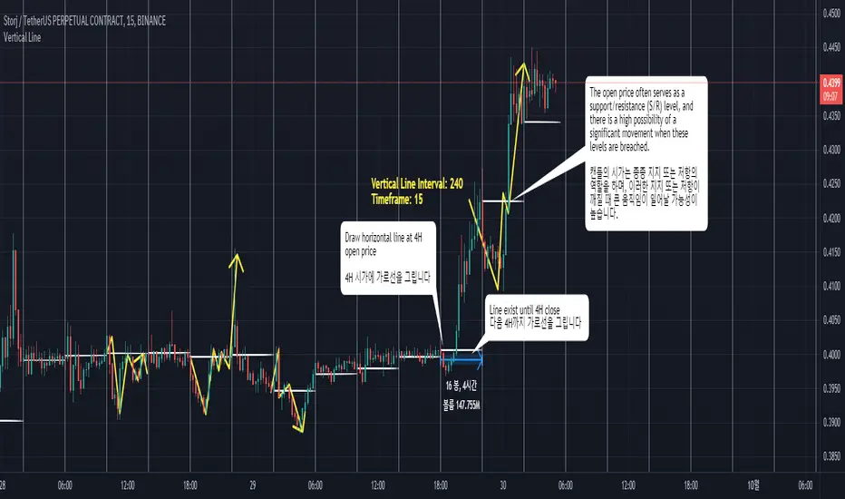
This script operates by drawing vertical lines at intervals defined by the user. Users can select the interval for the vertical lines in minutes, and the script automatically places vertical lines at each interval on the chart. For instance, if a 15-minute interval is selected, vertical lines will appear at the start and end times of every 15-minute candle on the chart.
Additionally, this script includes a feature that allows drawing horizontal lines representing the open price of the candles at each vertical line. This is crucial for traders observing price action around specific times and evaluating market conditions at regular intervals.
This script is operative across diverse time frames and can be adjusted to fit various trading styles and analyses. It is efficient, user-friendly, and adaptable to the diverse needs of traders.
The open price of a candle often serves as a support or resistance, and there is a high possibility of significant movement occurring when these S/R levels are breached.
How to Use
VLInterval: Users can input the interval for the vertical lines in minutes and select from 5, 15, 30, 60, 120, 240, 1440.
visibleTimeframe: Users can select the desired time frame where the vertical lines will be visible.
Color and Style: Users can freely modify the color and style of the lines.
Apply the indicator to the chart.
Select the desired interval for the vertical lines.
Adjust the visibility and style of the lines as needed.
By adhering to these steps, traders can effectively incorporate this tool into their analysis, maximizing the utility of interval-based evaluations and observations.
소개
간격 수직 선 그리기 도구는 트레이더가 차트에서 특정 간격을 시각화할 수 있도록 도와주는 지표입니다. 이 스크립트는 트레이더들이 다양한 시간 프레임에서 더 정확한 분석을 수행할 수 있게 해줍니다.
작동 원리
이 스크립트는 사용자가 정의한 간격에서 수직선을 그리는 방식으로 작동합니다. 사용자는 분 단위로 수직선 간격을 선택할 수 있고, 스크립트는 자동으로 차트의 각 간격에 수직선을 배치합니다. 예를 들어, 15분 간격이 선택되면, 차트에는 15분봉의 시작, 종료 시간마다 수직선이 나타납니다.
더불어, 이 스크립트는 각 수직선에서의 캔들의 시가를 나타내는 수평선을 그릴 수 있는 기능도 포함하고 있습니다. 이는 트레이더가 특정 시간 주변의 가격 행동을 관찰하고 정기적인 간격으로 시장 상황을 평가하는데 중요합니다.
이 스크립트는 다양한 시간 프레임에서 작동하며, 다양한 거래 스타일과 분석에 맞게 조정할 수 있습니다. 이는 효율적이고 사용자 친화적이며, 트레이더의 다양한 필요에 적응할 수 있습니다.
캔들의 시작가는 종종 지지 또는 저항의 역할을 하며, S/R이 깨질 때 큰 움직임이 일어날 가능성이 높습니다.
사용 방법
VLInterval: 사용자는 분 단위로 수직선 간격을 입력할 수 있으며, 5, 15, 30, 60, 120, 240, 1440 중에서 선택할 수 있습니다.
visibleTimeframe: 사용자는 수직선이 보이게 될 원하는 시간 프레임을 선택할 수 있습니다.
색상과 스타일: 사용자는 선의 색상과 스타일을 자유롭게 수정할 수 있습니다.
지표를 차트에 적용합니다.
수직선의 원하는 간격을 선택합니다.
선의 가시성과 스타일을 필요에 맞게 조정합니다.
Cerca negli script per "美国要强买强卖,要求中国购买指定商品,四年还必须买够15万亿?"
Previous Day High Low Strategy only for LongWelcome to the "Previous Day High Low Strategy only for Long"!.
This strategy aims to identify potential long trading opportunities based on the previous day's high and low prices, along with certain market strength conditions.
Key Features:
Entry Conditions: The strategy triggers a long position when the current day's closing price crosses above the previous day's high or low.
Market Strength Filter: The strategy incorporates a market strength filter using the Average Directional Index (ADX). It only takes long positions when the ADX value is above a specific threshold and when there is a predominance of upward movement.
Trade Timing: The strategy operates within a specified trade window, starting at 09:30 and ending at 15:10. Positions are closed at 15:15 if still active.
Risk Management: The strategy employs dynamic stop-loss and profit-taking levels based on a user-defined Max Profit value. It has three profit targets (T1, T2, T3) and a stop-loss level to manage risk effectively.
Rules:
Ensure that the strategy idea is clearly understandable. Provide an easy-to-read title and a thoughtful description explaining the reasoning behind the strategy.
All content should be ad-free. Avoid any form of promotion, advertising, or solicitation.
No fundraising requests or money solicitation is allowed on TradingView.
Publish in the same language as the TradingView subdomain you're on, except for script titles, which must be in English.
Don't plagiarize. Create and share only unique content, and always give credit when using someone else's work.
Be respectful, kind, and constructive when engaging with others.
Zero tolerance for contentious political discourse, defamatory, threatening, or discriminatory remarks.
Avoid sharing harmful, misleading, or inappropriate content.
Respect the moderators' work and address complaints privately.
Use only your original account and avoid creating duplicate or fake accounts.
Do not attempt to manipulate the reputation system or engage in like-for-like schemes.
Explanation of how the strategy works
1. Previous Day's High and Low (HH, LL):
In this strategy, we start by obtaining the high and low prices of the previous day (not the current day) using the request.security function. This function allows us to access historical data for a specific time frame. The high and low prices are stored in the variables HH and LL, respectively.
2. Entry Conditions:
The strategy uses two conditions to trigger a long position:
Condition 1 (Long Condition 1): If the closing price of the current day crosses above the previous day's high (HH), it generates a long signal. This is achieved using the ta.crossover function, which detects when a crossover occurs.
Condition 2 (Long Condition 2): Similarly, if the closing price of the current day crosses above the previous day's low (LL), it also generates a long signal.
Combined Condition: To take long positions, the strategy combines both long conditions using the logical OR operator (or). This means that if either of the two conditions is met, a long position will be initiated.
3. Market Strength Filter:
The strategy also includes a filter based on the Average Directional Index (ADX) to gauge the market's strength before taking long positions. The ADX measures the strength of a trend in the market. The higher the ADX value, the stronger the trend.
Calculation of ADX: The ADX is calculated using the adx function, which takes two parameters: LWdilength (DMI Length) and LWadxlength (ADX period).
Strength Condition (strength_up): The strategy requires that the ADX value should be above a threshold (11 in this case) and that there is a predominance of upward movement (up > down) before initiating a long position. The LWADX value is multiplied by 2.5 and compared to the highest value of LWADX from the last 4 periods using ta.highest(LWADX , 4). If these conditions are met, the variable strength_up is set to true.
Combined Condition: The strength_up condition is then combined with the long conditions using the logical AND operator (and). This means that the strategy will only take a long position if both the long conditions and the market strength condition are met.
4. Trade Timing:
The strategy sets a specific trade window between 09:30 and 15:10. It will only execute trades within this time frame (TradeTime).
5. Risk Management:
The strategy implements dynamic stop-loss (SL) and profit-taking levels (T1, T2, T3) based on a user-defined Max Profit value. The stop-loss is set as a percentage of the Max Profit value. As the position moves in favor of the trader, the profit targets are adjusted accordingly.
6. Position Management:
The strategy uses the strategy.entry function to enter long positions based on the combined entry conditions. Once a position is open, the script uses strategy.exit to define the exit condition when either the profit target or stop-loss level is hit. The strategy.close function is used to close any open position at the end of the trade window (15:15).
7. Plotting:
The strategy uses the plot function to visualize the previous day's high and low prices, as well as the stop-loss (SL) and profit-taking (T1, T2, T3) levels on the chart.
Overall, the "Previous Day High Low Strategy only for Long" aims to identify potential long trading opportunities based on the previous day's price action and market strength conditions. However, as with any trading strategy, it's essential to thoroughly test it and consider risk management before applying it to real-world trading scenarios.
Disclaimer:
The information presented by this strategy is for educational purposes only and should not be considered as investment advice. The strategy is not designed for qualified investors. Always conduct your own research and consult with a financial advisor before making any trading decisions.
Remember, the success of any trading strategy depends on various factors, including market conditions, risk management, and individual trading skills. Past performance is not indicative of future results.

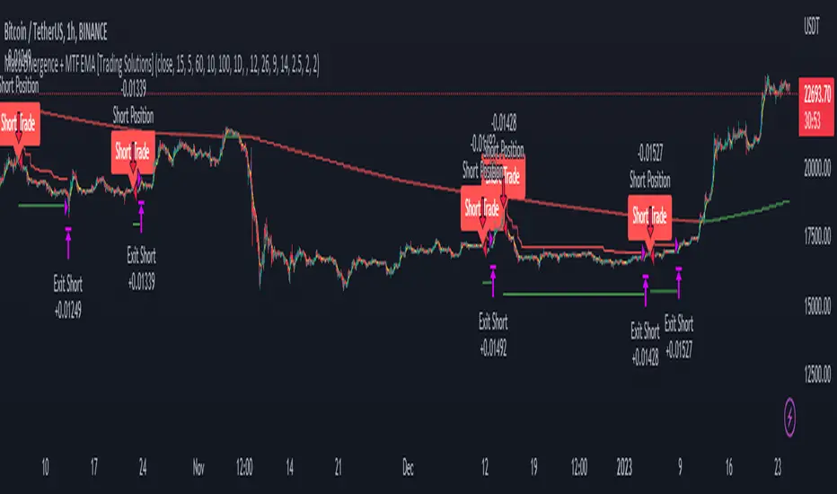
Macd Divergence + MTF EMA MACD Divergence + Multi Time Frame EMA
This Strategy uses 3 indicators: the Macd and two emas in different time frames
The configuration of the strategy is:
Macd standar configuration (12, 26, 9) in 1H resolution
10 periods ema, in 1H resolution
5 periods ema, in 15 minutes resolution
We use the two emas to filter for long and short positions.
If 15 minutes ema is above 1H ema, we look for long positions
If 15 minutes ema is below 1H ema, we look for short positions
We can use an aditional filter using a 100 days ema, so when the 15' and 1H emas are above the daily ema we take long positions
Using this filter improves the strategy
We wait for Macd indicator to form a divergence between histogram and price
If we have a bullish divergence, and 15 minutes ema is above 1H ema, we wait for macd line to cross above signal line and we open a long position
If we have a bearish divergence, and 15 minutes ema is below 1H ema, we wait for macd line to cross below signal line and we open a short position
We close both position after a cross in the oposite direction of macd line and signal line
Also we can configure a Take profit parameter and a trailing stop loss
PINAKI__RSI M/W/D/H/15 (Top Right, Padding)display monthly, weekly, daily, 1Hr, 15Min RSI in single frame
Kelly Position Size CalculatorThis position sizing calculator implements the Kelly Criterion, developed by John L. Kelly Jr. at Bell Laboratories in 1956, to determine mathematically optimal position sizes for maximizing long-term wealth growth. Unlike arbitrary position sizing methods, this tool provides a scientifically solution based on your strategy's actual performance statistics and incorporates modern refinements from over six decades of academic research.
The Kelly Criterion addresses a fundamental question in capital allocation: "What fraction of capital should be allocated to each opportunity to maximize growth while avoiding ruin?" This question has profound implications for financial markets, where traders and investors constantly face decisions about optimal capital allocation (Van Tharp, 2007).
Theoretical Foundation
The Kelly Criterion for binary outcomes is expressed as f* = (bp - q) / b, where f* represents the optimal fraction of capital to allocate, b denotes the risk-reward ratio, p indicates the probability of success, and q represents the probability of loss (Kelly, 1956). This formula maximizes the expected logarithm of wealth, ensuring maximum long-term growth rate while avoiding the risk of ruin.
The mathematical elegance of Kelly's approach lies in its derivation from information theory. Kelly's original work was motivated by Claude Shannon's information theory (Shannon, 1948), recognizing that maximizing the logarithm of wealth is equivalent to maximizing the rate of information transmission. This connection between information theory and wealth accumulation provides a deep theoretical foundation for optimal position sizing.
The logarithmic utility function underlying the Kelly Criterion naturally embodies several desirable properties for capital management. It exhibits decreasing marginal utility, penalizes large losses more severely than it rewards equivalent gains, and focuses on geometric rather than arithmetic mean returns, which is appropriate for compounding scenarios (Thorp, 2006).
Scientific Implementation
This calculator extends beyond basic Kelly implementation by incorporating state of the art refinements from academic research:
Parameter Uncertainty Adjustment: Following Michaud (1989), the implementation applies Bayesian shrinkage to account for parameter estimation error inherent in small sample sizes. The adjustment formula f_adjusted = f_kelly × confidence_factor + f_conservative × (1 - confidence_factor) addresses the overconfidence bias documented by Baker and McHale (2012), where the confidence factor increases with sample size and the conservative estimate equals 0.25 (quarter Kelly).
Sample Size Confidence: The reliability of Kelly calculations depends critically on sample size. Research by Browne and Whitt (1996) provides theoretical guidance on minimum sample requirements, suggesting that at least 30 independent observations are necessary for meaningful parameter estimates, with 100 or more trades providing reliable estimates for most trading strategies.
Universal Asset Compatibility: The calculator employs intelligent asset detection using TradingView's built-in symbol information, automatically adapting calculations for different asset classes without manual configuration.
ASSET SPECIFIC IMPLEMENTATION
Equity Markets: For stocks and ETFs, position sizing follows the calculation Shares = floor(Kelly Fraction × Account Size / Share Price). This straightforward approach reflects whole share constraints while accommodating fractional share trading capabilities.
Foreign Exchange Markets: Forex markets require lot-based calculations following Lot Size = Kelly Fraction × Account Size / (100,000 × Base Currency Value). The calculator automatically handles major currency pairs with appropriate pip value calculations, following industry standards described by Archer (2010).
Futures Markets: Futures position sizing accounts for leverage and margin requirements through Contracts = floor(Kelly Fraction × Account Size / Margin Requirement). The calculator estimates margin requirements as a percentage of contract notional value, with specific adjustments for micro-futures contracts that have smaller sizes and reduced margin requirements (Kaufman, 2013).
Index and Commodity Markets: These markets combine characteristics of both equity and futures markets. The calculator automatically detects whether instruments are cash-settled or futures-based, applying appropriate sizing methodologies with correct point value calculations.
Risk Management Integration
The calculator integrates sophisticated risk assessment through two primary modes:
Stop Loss Integration: When fixed stop-loss levels are defined, risk calculation follows Risk per Trade = Position Size × Stop Loss Distance. This ensures that the Kelly fraction accounts for actual risk exposure rather than theoretical maximum loss, with stop-loss distance measured in appropriate units for each asset class.
Strategy Drawdown Assessment: For discretionary exit strategies, risk estimation uses maximum historical drawdown through Risk per Trade = Position Value × (Maximum Drawdown / 100). This approach assumes that individual trade losses will not exceed the strategy's historical maximum drawdown, providing a reasonable estimate for strategies with well-defined risk characteristics.
Fractional Kelly Approaches
Pure Kelly sizing can produce substantial volatility, leading many practitioners to adopt fractional Kelly approaches. MacLean, Sanegre, Zhao, and Ziemba (2004) analyze the trade-offs between growth rate and volatility, demonstrating that half-Kelly typically reduces volatility by approximately 75% while sacrificing only 25% of the growth rate.
The calculator provides three primary Kelly modes to accommodate different risk preferences and experience levels. Full Kelly maximizes growth rate while accepting higher volatility, making it suitable for experienced practitioners with strong risk tolerance and robust capital bases. Half Kelly offers a balanced approach popular among professional traders, providing optimal risk-return balance by reducing volatility significantly while maintaining substantial growth potential. Quarter Kelly implements a conservative approach with low volatility, recommended for risk-averse traders or those new to Kelly methodology who prefer gradual introduction to optimal position sizing principles.
Empirical Validation and Performance
Extensive academic research supports the theoretical advantages of Kelly sizing. Hakansson and Ziemba (1995) provide a comprehensive review of Kelly applications in finance, documenting superior long-term performance across various market conditions and asset classes. Estrada (2008) analyzes Kelly performance in international equity markets, finding that Kelly-based strategies consistently outperform fixed position sizing approaches over extended periods across 19 developed markets over a 30-year period.
Several prominent investment firms have successfully implemented Kelly-based position sizing. Pabrai (2007) documents the application of Kelly principles at Berkshire Hathaway, noting Warren Buffett's concentrated portfolio approach aligns closely with Kelly optimal sizing for high-conviction investments. Quantitative hedge funds, including Renaissance Technologies and AQR, have incorporated Kelly-based risk management into their systematic trading strategies.
Practical Implementation Guidelines
Successful Kelly implementation requires systematic application with attention to several critical factors:
Parameter Estimation: Accurate parameter estimation represents the greatest challenge in practical Kelly implementation. Brown (1976) notes that small errors in probability estimates can lead to significant deviations from optimal performance. The calculator addresses this through Bayesian adjustments and confidence measures.
Sample Size Requirements: Users should begin with conservative fractional Kelly approaches until achieving sufficient historical data. Strategies with fewer than 30 trades may produce unreliable Kelly estimates, regardless of adjustments. Full confidence typically requires 100 or more independent trade observations.
Market Regime Considerations: Parameters that accurately describe historical performance may not reflect future market conditions. Ziemba (2003) recommends regular parameter updates and conservative adjustments when market conditions change significantly.
Professional Features and Customization
The calculator provides comprehensive customization options for professional applications:
Multiple Color Schemes: Eight professional color themes (Gold, EdgeTools, Behavioral, Quant, Ocean, Fire, Matrix, Arctic) with dark and light theme compatibility ensure optimal visibility across different trading environments.
Flexible Display Options: Adjustable table size and position accommodate various chart layouts and user preferences, while maintaining analytical depth and clarity.
Comprehensive Results: The results table presents essential information including asset specifications, strategy statistics, Kelly calculations, sample confidence measures, position values, risk assessments, and final position sizes in appropriate units for each asset class.
Limitations and Considerations
Like any analytical tool, the Kelly Criterion has important limitations that users must understand:
Stationarity Assumption: The Kelly Criterion assumes that historical strategy statistics represent future performance characteristics. Non-stationary market conditions may invalidate this assumption, as noted by Lo and MacKinlay (1999).
Independence Requirement: Each trade should be independent to avoid correlation effects. Many trading strategies exhibit serial correlation in returns, which can affect optimal position sizing and may require adjustments for portfolio applications.
Parameter Sensitivity: Kelly calculations are sensitive to parameter accuracy. Regular calibration and conservative approaches are essential when parameter uncertainty is high.
Transaction Costs: The implementation incorporates user-defined transaction costs but assumes these remain constant across different position sizes and market conditions, following Ziemba (2003).
Advanced Applications and Extensions
Multi-Asset Portfolio Considerations: While this calculator optimizes individual position sizes, portfolio-level applications require additional considerations for correlation effects and aggregate risk management. Simplified portfolio approaches include treating positions independently with correlation adjustments.
Behavioral Factors: Behavioral finance research reveals systematic biases that can interfere with Kelly implementation. Kahneman and Tversky (1979) document loss aversion, overconfidence, and other cognitive biases that lead traders to deviate from optimal strategies. Successful implementation requires disciplined adherence to calculated recommendations.
Time-Varying Parameters: Advanced implementations may incorporate time-varying parameter models that adjust Kelly recommendations based on changing market conditions, though these require sophisticated econometric techniques and substantial computational resources.
Comprehensive Usage Instructions and Practical Examples
Implementation begins with loading the calculator on your desired trading instrument's chart. The system automatically detects asset type across stocks, forex, futures, and cryptocurrency markets while extracting current price information. Navigation to the indicator settings allows input of your specific strategy parameters.
Strategy statistics configuration requires careful attention to several key metrics. The win rate should be calculated from your backtest results using the formula of winning trades divided by total trades multiplied by 100. Average win represents the sum of all profitable trades divided by the number of winning trades, while average loss calculates the sum of all losing trades divided by the number of losing trades, entered as a positive number. The total historical trades parameter requires the complete number of trades in your backtest, with a minimum of 30 trades recommended for basic functionality and 100 or more trades optimal for statistical reliability. Account size should reflect your available trading capital, specifically the risk capital allocated for trading rather than total net worth.
Risk management configuration adapts to your specific trading approach. The stop loss setting should be enabled if you employ fixed stop-loss exits, with the stop loss distance specified in appropriate units depending on the asset class. For stocks, this distance is measured in dollars, for forex in pips, and for futures in ticks. When stop losses are not used, the maximum strategy drawdown percentage from your backtest provides the risk assessment baseline. Kelly mode selection offers three primary approaches: Full Kelly for aggressive growth with higher volatility suitable for experienced practitioners, Half Kelly for balanced risk-return optimization popular among professional traders, and Quarter Kelly for conservative approaches with reduced volatility.
Display customization ensures optimal integration with your trading environment. Eight professional color themes provide optimization for different chart backgrounds and personal preferences. Table position selection allows optimal placement within your chart layout, while table size adjustment ensures readability across different screen resolutions and viewing preferences.
Detailed Practical Examples
Example 1: SPY Swing Trading Strategy
Consider a professionally developed swing trading strategy for SPY (S&P 500 ETF) with backtesting results spanning 166 total trades. The strategy achieved 110 winning trades, representing a 66.3% win rate, with an average winning trade of $2,200 and average losing trade of $862. The maximum drawdown reached 31.4% during the testing period, and the available trading capital amounts to $25,000. This strategy employs discretionary exits without fixed stop losses.
Implementation requires loading the calculator on the SPY daily chart and configuring the parameters accordingly. The win rate input receives 66.3, while average win and loss inputs receive 2200 and 862 respectively. Total historical trades input requires 166, with account size set to 25000. The stop loss function remains disabled due to the discretionary exit approach, with maximum strategy drawdown set to 31.4%. Half Kelly mode provides the optimal balance between growth and risk management for this application.
The calculator generates several key outputs for this scenario. The risk-reward ratio calculates automatically to 2.55, while the Kelly fraction reaches approximately 53% before scientific adjustments. Sample confidence achieves 100% given the 166 trades providing high statistical confidence. The recommended position settles at approximately 27% after Half Kelly and Bayesian adjustment factors. Position value reaches approximately $6,750, translating to 16 shares at a $420 SPY price. Risk per trade amounts to approximately $2,110, representing 31.4% of position value, with expected value per trade reaching approximately $1,466. This recommendation represents the mathematically optimal balance between growth potential and risk management for this specific strategy profile.
Example 2: EURUSD Day Trading with Stop Losses
A high-frequency EURUSD day trading strategy demonstrates different parameter requirements compared to swing trading approaches. This strategy encompasses 89 total trades with a 58% win rate, generating an average winning trade of $180 and average losing trade of $95. The maximum drawdown reached 12% during testing, with available capital of $10,000. The strategy employs fixed stop losses at 25 pips and take profit targets at 45 pips, providing clear risk-reward parameters.
Implementation begins with loading the calculator on the EURUSD 1-hour chart for appropriate timeframe alignment. Parameter configuration includes win rate at 58, average win at 180, and average loss at 95. Total historical trades input receives 89, with account size set to 10000. The stop loss function is enabled with distance set to 25 pips, reflecting the fixed exit strategy. Quarter Kelly mode provides conservative positioning due to the smaller sample size compared to the previous example.
Results demonstrate the impact of smaller sample sizes on Kelly calculations. The risk-reward ratio calculates to 1.89, while the Kelly fraction reaches approximately 32% before adjustments. Sample confidence achieves 89%, providing moderate statistical confidence given the 89 trades. The recommended position settles at approximately 7% after Quarter Kelly application and Bayesian shrinkage adjustment for the smaller sample. Position value amounts to approximately $700, translating to 0.07 standard lots. Risk per trade reaches approximately $175, calculated as 25 pips multiplied by lot size and pip value, with expected value per trade at approximately $49. This conservative position sizing reflects the smaller sample size, with position sizes expected to increase as trade count surpasses 100 and statistical confidence improves.
Example 3: ES1! Futures Systematic Strategy
Systematic futures trading presents unique considerations for Kelly criterion application, as demonstrated by an E-mini S&P 500 futures strategy encompassing 234 total trades. This systematic approach achieved a 45% win rate with an average winning trade of $1,850 and average losing trade of $720. The maximum drawdown reached 18% during the testing period, with available capital of $50,000. The strategy employs 15-tick stop losses with contract specifications of $50 per tick, providing precise risk control mechanisms.
Implementation involves loading the calculator on the ES1! 15-minute chart to align with the systematic trading timeframe. Parameter configuration includes win rate at 45, average win at 1850, and average loss at 720. Total historical trades receives 234, providing robust statistical foundation, with account size set to 50000. The stop loss function is enabled with distance set to 15 ticks, reflecting the systematic exit methodology. Half Kelly mode balances growth potential with appropriate risk management for futures trading.
Results illustrate how favorable risk-reward ratios can support meaningful position sizing despite lower win rates. The risk-reward ratio calculates to 2.57, while the Kelly fraction reaches approximately 16%, lower than previous examples due to the sub-50% win rate. Sample confidence achieves 100% given the 234 trades providing high statistical confidence. The recommended position settles at approximately 8% after Half Kelly adjustment. Estimated margin per contract amounts to approximately $2,500, resulting in a single contract allocation. Position value reaches approximately $2,500, with risk per trade at $750, calculated as 15 ticks multiplied by $50 per tick. Expected value per trade amounts to approximately $508. Despite the lower win rate, the favorable risk-reward ratio supports meaningful position sizing, with single contract allocation reflecting appropriate leverage management for futures trading.
Example 4: MES1! Micro-Futures for Smaller Accounts
Micro-futures contracts provide enhanced accessibility for smaller trading accounts while maintaining identical strategy characteristics. Using the same systematic strategy statistics from the previous example but with available capital of $15,000 and micro-futures specifications of $5 per tick with reduced margin requirements, the implementation demonstrates improved position sizing granularity.
Kelly calculations remain identical to the full-sized contract example, maintaining the same risk-reward dynamics and statistical foundations. However, estimated margin per contract reduces to approximately $250 for micro-contracts, enabling allocation of 4-5 micro-contracts. Position value reaches approximately $1,200, while risk per trade calculates to $75, derived from 15 ticks multiplied by $5 per tick. This granularity advantage provides better position size precision for smaller accounts, enabling more accurate Kelly implementation without requiring large capital commitments.
Example 5: Bitcoin Swing Trading
Cryptocurrency markets present unique challenges requiring modified Kelly application approaches. A Bitcoin swing trading strategy on BTCUSD encompasses 67 total trades with a 71% win rate, generating average winning trades of $3,200 and average losing trades of $1,400. Maximum drawdown reached 28% during testing, with available capital of $30,000. The strategy employs technical analysis for exits without fixed stop losses, relying on price action and momentum indicators.
Implementation requires conservative approaches due to cryptocurrency volatility characteristics. Quarter Kelly mode is recommended despite the high win rate to account for crypto market unpredictability. Expected position sizing remains reduced due to the limited sample size of 67 trades, requiring additional caution until statistical confidence improves. Regular parameter updates are strongly recommended due to cryptocurrency market evolution and changing volatility patterns that can significantly impact strategy performance characteristics.
Advanced Usage Scenarios
Portfolio position sizing requires sophisticated consideration when running multiple strategies simultaneously. Each strategy should have its Kelly fraction calculated independently to maintain mathematical integrity. However, correlation adjustments become necessary when strategies exhibit related performance patterns. Moderately correlated strategies should receive individual position size reductions of 10-20% to account for overlapping risk exposure. Aggregate portfolio risk monitoring ensures total exposure remains within acceptable limits across all active strategies. Professional practitioners often consider using lower fractional Kelly approaches, such as Quarter Kelly, when running multiple strategies simultaneously to provide additional safety margins.
Parameter sensitivity analysis forms a critical component of professional Kelly implementation. Regular validation procedures should include monthly parameter updates using rolling 100-trade windows to capture evolving market conditions while maintaining statistical relevance. Sensitivity testing involves varying win rates by ±5% and average win/loss ratios by ±10% to assess recommendation stability under different parameter assumptions. Out-of-sample validation reserves 20% of historical data for parameter verification, ensuring that optimization doesn't create curve-fitted results. Regime change detection monitors actual performance against expected metrics, triggering parameter reassessment when significant deviations occur.
Risk management integration requires professional overlay considerations beyond pure Kelly calculations. Daily loss limits should cease trading when daily losses exceed twice the calculated risk per trade, preventing emotional decision-making during adverse periods. Maximum position limits should never exceed 25% of account value in any single position regardless of Kelly recommendations, maintaining diversification principles. Correlation monitoring reduces position sizes when holding multiple correlated positions that move together during market stress. Volatility adjustments consider reducing position sizes during periods of elevated VIX above 25 for equity strategies, adapting to changing market conditions.
Troubleshooting and Optimization
Professional implementation often encounters specific challenges requiring systematic troubleshooting approaches. Zero position size displays typically result from insufficient capital for minimum position sizes, negative expected values, or extremely conservative Kelly calculations. Solutions include increasing account size, verifying strategy statistics for accuracy, considering Quarter Kelly mode for conservative approaches, or reassessing overall strategy viability when fundamental issues exist.
Extremely high Kelly fractions exceeding 50% usually indicate underlying problems with parameter estimation. Common causes include unrealistic win rates, inflated risk-reward ratios, or curve-fitted backtest results that don't reflect genuine trading conditions. Solutions require verifying backtest methodology, including all transaction costs in calculations, testing strategies on out-of-sample data, and using conservative fractional Kelly approaches until parameter reliability improves.
Low sample confidence below 50% reflects insufficient historical trades for reliable parameter estimation. This situation demands gathering additional trading data, using Quarter Kelly approaches until reaching 100 or more trades, applying extra conservatism in position sizing, and considering paper trading to build statistical foundations without capital risk.
Inconsistent results across similar strategies often stem from parameter estimation differences, market regime changes, or strategy degradation over time. Professional solutions include standardizing backtest methodology across all strategies, updating parameters regularly to reflect current conditions, and monitoring live performance against expectations to identify deteriorating strategies.
Position sizes that appear inappropriately large or small require careful validation against traditional risk management principles. Professional standards recommend never risking more than 2-3% per trade regardless of Kelly calculations. Calibration should begin with Quarter Kelly approaches, gradually increasing as comfort and confidence develop. Most institutional traders utilize 25-50% of full Kelly recommendations to balance growth with prudent risk management.
Market condition adjustments require dynamic approaches to Kelly implementation. Trending markets may support full Kelly recommendations when directional momentum provides favorable conditions. Ranging or volatile markets typically warrant reducing to Half or Quarter Kelly to account for increased uncertainty. High correlation periods demand reducing individual position sizes when multiple positions move together, concentrating risk exposure. News and event periods often justify temporary position size reductions during high-impact releases that can create unpredictable market movements.
Performance monitoring requires systematic protocols to ensure Kelly implementation remains effective over time. Weekly reviews should compare actual versus expected win rates and average win/loss ratios to identify parameter drift or strategy degradation. Position size efficiency and execution quality monitoring ensures that calculated recommendations translate effectively into actual trading results. Tracking correlation between calculated and realized risk helps identify discrepancies between theoretical and practical risk exposure.
Monthly calibration provides more comprehensive parameter assessment using the most recent 100 trades to maintain statistical relevance while capturing current market conditions. Kelly mode appropriateness requires reassessment based on recent market volatility and performance characteristics, potentially shifting between Full, Half, and Quarter Kelly approaches as conditions change. Transaction cost evaluation ensures that commission structures, spreads, and slippage estimates remain accurate and current.
Quarterly strategic reviews encompass comprehensive strategy performance analysis comparing long-term results against expectations and identifying trends in effectiveness. Market regime assessment evaluates parameter stability across different market conditions, determining whether strategy characteristics remain consistent or require fundamental adjustments. Strategic modifications to position sizing methodology may become necessary as markets evolve or trading approaches mature, ensuring that Kelly implementation continues supporting optimal capital allocation objectives.
Professional Applications
This calculator serves diverse professional applications across the financial industry. Quantitative hedge funds utilize the implementation for systematic position sizing within algorithmic trading frameworks, where mathematical precision and consistent application prove essential for institutional capital management. Professional discretionary traders benefit from optimized position management that removes emotional bias while maintaining flexibility for market-specific adjustments. Portfolio managers employ the calculator for developing risk-adjusted allocation strategies that enhance returns while maintaining prudent risk controls across diverse asset classes and investment strategies.
Individual traders seeking mathematical optimization of capital allocation find the calculator provides institutional-grade methodology previously available only to professional money managers. The Kelly Criterion establishes theoretical foundation for optimal capital allocation across both single strategies and multiple trading systems, offering significant advantages over arbitrary position sizing methods that rely on intuition or fixed percentage approaches. Professional implementation ensures consistent application of mathematically sound principles while adapting to changing market conditions and strategy performance characteristics.
Conclusion
The Kelly Criterion represents one of the few mathematically optimal solutions to fundamental investment problems. When properly understood and carefully implemented, it provides significant competitive advantage in financial markets. This calculator implements modern refinements to Kelly's original formula while maintaining accessibility for practical trading applications.
Success with Kelly requires ongoing learning, systematic application, and continuous refinement based on market feedback and evolving research. Users who master Kelly principles and implement them systematically can expect superior risk-adjusted returns and more consistent capital growth over extended periods.
The extensive academic literature provides rich resources for deeper study, while practical experience builds the intuition necessary for effective implementation. Regular parameter updates, conservative approaches with limited data, and disciplined adherence to calculated recommendations are essential for optimal results.
References
Archer, M. D. (2010). Getting Started in Currency Trading: Winning in Today's Forex Market (3rd ed.). John Wiley & Sons.
Baker, R. D., & McHale, I. G. (2012). An empirical Bayes approach to optimising betting strategies. Journal of the Royal Statistical Society: Series D (The Statistician), 61(1), 75-92.
Breiman, L. (1961). Optimal gambling systems for favorable games. In J. Neyman (Ed.), Proceedings of the Fourth Berkeley Symposium on Mathematical Statistics and Probability (pp. 65-78). University of California Press.
Brown, D. B. (1976). Optimal portfolio growth: Logarithmic utility and the Kelly criterion. In W. T. Ziemba & R. G. Vickson (Eds.), Stochastic Optimization Models in Finance (pp. 1-23). Academic Press.
Browne, S., & Whitt, W. (1996). Portfolio choice and the Bayesian Kelly criterion. Advances in Applied Probability, 28(4), 1145-1176.
Estrada, J. (2008). Geometric mean maximization: An overlooked portfolio approach? The Journal of Investing, 17(4), 134-147.
Hakansson, N. H., & Ziemba, W. T. (1995). Capital growth theory. In R. A. Jarrow, V. Maksimovic, & W. T. Ziemba (Eds.), Handbooks in Operations Research and Management Science (Vol. 9, pp. 65-86). Elsevier.
Kahneman, D., & Tversky, A. (1979). Prospect theory: An analysis of decision under risk. Econometrica, 47(2), 263-291.
Kaufman, P. J. (2013). Trading Systems and Methods (5th ed.). John Wiley & Sons.
Kelly Jr, J. L. (1956). A new interpretation of information rate. Bell System Technical Journal, 35(4), 917-926.
Lo, A. W., & MacKinlay, A. C. (1999). A Non-Random Walk Down Wall Street. Princeton University Press.
MacLean, L. C., Sanegre, E. O., Zhao, Y., & Ziemba, W. T. (2004). Capital growth with security. Journal of Economic Dynamics and Control, 28(4), 937-954.
MacLean, L. C., Thorp, E. O., & Ziemba, W. T. (2011). The Kelly Capital Growth Investment Criterion: Theory and Practice. World Scientific.
Michaud, R. O. (1989). The Markowitz optimization enigma: Is 'optimized' optimal? Financial Analysts Journal, 45(1), 31-42.
Pabrai, M. (2007). The Dhandho Investor: The Low-Risk Value Method to High Returns. John Wiley & Sons.
Shannon, C. E. (1948). A mathematical theory of communication. Bell System Technical Journal, 27(3), 379-423.
Tharp, V. K. (2007). Trade Your Way to Financial Freedom (2nd ed.). McGraw-Hill.
Thorp, E. O. (2006). The Kelly criterion in blackjack sports betting, and the stock market. In L. C. MacLean, E. O. Thorp, & W. T. Ziemba (Eds.), The Kelly Capital Growth Investment Criterion: Theory and Practice (pp. 789-832). World Scientific.
Van Tharp, K. (2007). Trade Your Way to Financial Freedom (2nd ed.). McGraw-Hill Education.
Vince, R. (1992). The Mathematics of Money Management: Risk Analysis Techniques for Traders. John Wiley & Sons.
Vince, R., & Zhu, H. (2015). Optimal betting under parameter uncertainty. Journal of Statistical Planning and Inference, 161, 19-31.
Ziemba, W. T. (2003). The Stochastic Programming Approach to Asset, Liability, and Wealth Management. The Research Foundation of AIMR.
Further Reading
For comprehensive understanding of Kelly Criterion applications and advanced implementations:
MacLean, L. C., Thorp, E. O., & Ziemba, W. T. (2011). The Kelly Capital Growth Investment Criterion: Theory and Practice. World Scientific.
Vince, R. (1992). The Mathematics of Money Management: Risk Analysis Techniques for Traders. John Wiley & Sons.
Thorp, E. O. (2017). A Man for All Markets: From Las Vegas to Wall Street. Random House.
Cover, T. M., & Thomas, J. A. (2006). Elements of Information Theory (2nd ed.). John Wiley & Sons.
Ziemba, W. T., & Vickson, R. G. (Eds.). (2006). Stochastic Optimization Models in Finance. World Scientific.

Dual Session ORB S/R Lines Pro by Yendor_BShort description:
Clean opening-range breakout support/resistance lines for London and US sessions with confirmed breakout labels and alert-ready signals. UTC-based, adjustable start point, customizable styling, minimal clutter.
Detailed description:
What it does:
Captures the Opening Range (default first 15 minutes) for London and New York (US) sessions in UTC, plots the high and low as support/resistance lines, and marks confirmed breakouts when price closes beyond those levels. Lines can begin at either the range end or session start and persist for the configured session length.
Key Features:
ORB defined over the first N minutes after session open (configurable, default 15).
Two sessions: London and US (New York) with separate start times.
High/low support & resistance lines per session:
Selectable start point: Range End or Session Start.
Independently customizable color, width, and style (solid/dashed/dotted) for each high and low.
Confirmed breakout labels: only on the first candle that closes beyond the ORB high or low after the range completes (prior close must be inside).
Alerts and alertconditions for breakout long/short per session, usable in TradingView’s alert dialog.
Fully UTC-based. Works on any timeframe; 1-minute or 5-minute recommended for precision.
Minimal visual clutter; no persistent shaded boxes in this version.
Inputs explained:
ORB Duration (minutes): Length of the opening range used to calculate session high and low.
Session Length (hours): How long the S/R lines remain active (typically full session).
London / US Start (UTC): Session open times in UTC.
Line Start Point: Choose whether the lines begin at the range end or at the session start.
High/Low Styling: Independent color, thickness, and style for each session’s high and low.
Breakout Labels: Toggle one-time confirmed breakout annotations.
Alerts: Enable breakout alert messages.
Example workflows:
Monitor the first 15 minutes of the London session.
After the range, wait for a candle to close beyond the high or low for a confirmed breakout.
Use the label or alert to trigger entry logic (retest, continuation, etc.).
Repeat for the US session; compare overlaps for higher conviction.
Alert setup:
Open the Alerts panel. Choose one of the built-in alertconditions: London Breakout Long, London Breakout Short, US Breakout Long, US Breakout Short. Set frequency to Once Per Bar Close. Customize notification/webhook payload if automating.
Preset suggestions:
Standard London ORB: 15 minute range, lines from range end, green high / lime low.
Standard US ORB: 15 minute range, lines from range end, blue high / aqua low.
Overlap Bias: Both sessions active, lines start from session start, differentiated styles.
Tips & best practices:
Combine with external volume or volatility filters to reduce false breakouts. Use on correlated pairs to observe consistent session structure. Treat broken ORB levels as flipped support/resistance on revisit. Prefer confirmed closes beyond lines rather than wick touches.
Limitations / disclaimer:
Provides structural visualization and breakout signaling; does not guarantee profitability. Always apply proper risk management and confirm with additional context. Backtest settings before live use.
Tags:
#ORB #OpeningRangeBreakout #SessionTrading #LondonSession #NewYorkSession #SupportResistance #Breakout #Intraday #Pinev6 #TradingView #Forex #TrendStructure #Alerts #USD #EURUSD #TradingSignals #UTCBased #PriceAction #MarketStructure #IntradayBreakouts

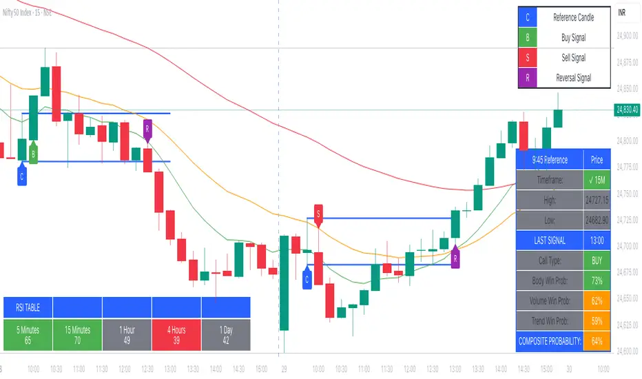
9:45am NIFTY TRADINGTime Frame: 15 Minutes | Reference Candle Time: 9:45 AM IST | Valid Trading Window: 3 Hours
📌 Introduction
This document outlines a structured trading strategy for NIFTY & BANKNIFTY Options based on a 15-minute timeframe with a 9:45 AM IST reference candle. The strategy incorporates technical indicators, probability analysis, and strict trading rules to optimize entries and exits.
📊 Core Features
1. Reference Time Trading System
9:45 AM IST Candle acts as the reference for the day.
All signals (Buy/Sell/Reversal) are generated based on price action relative to this candle.
The valid trading window is 3 hours after the reference candle.
2. Signal Generation Logic
Signal Condition
Buy (B) Price breaks above reference candle high with confirmation
Sell (S) Price breaks below reference candle low with confirmation
Reversal (R) Early trend reversal signal (requires strict confirmation)
3. Probability Analysis System
The strategy calculates Win Probability (%) using 4 components:
Component Weight Calculation
Body Win Probability 30% Based on candle body strength (body % of total range)
Volume Win Probability 30% Current volume vs. average volume strength
Trend Win Probability 40% EMA crossover + RSI momentum alignment
Composite Probability - Weighted average of all 3 components
Probability Color Coding:
🟢 Green (High Probability): ≥70%
🟠 Orange (Medium Probability): 50-69%
🔴 Red (Low Probability): <50%
4. Timeframe Enforcement
Strictly 15-minute charts only (no other timeframes allowed).
System auto-disables signals if the wrong timeframe is selected.
📈 Technical Analysis Components
1. EMA System (Trend Analysis)
Short EMA (9) – Fast trend indicator
Middle EMA (20) – Intermediate trend
Long EMA (50) – Long-term trend confirmation
Rules:
Buy Signal: Price > 9 EMA > 20 EMA > 50 EMA (Bullish trend)
Sell Signal: Price < 9 EMA < 20 EMA < 50 EMA (Bearish trend)
2. Multi-Timeframe RSI (Momentum)
5M, 15M, 1H, 4H, Daily RSI values are compared for divergence/confluence.
Overbought (≥70) / Oversold (≤30) conditions help in reversal signals.
3. Volume Analysis
Volume Strength (%) = (Current Volume / Avg. Volume) × 100
Strong Volume (>120% Avg.) confirms breakout/breakdown.
4. Body Percentage (Candle Strength)
Body % = (Close - Open) / (High - Low) × 100
Strong Bullish Candle: Body > 60%
Strong Bearish Candle: Body < 40%
📊 Visual Elements
1. Information Tables
Reference Data Table (9:45 AM Candle High/Low/Close)
RSI Values Table (5M, 15M, 1H, 4H, Daily)
Signal Legend (Buy/Sell/Reversal indicators)
2. Chart Overlays
Reference Lines (9:45 AM High & Low)
EMA Lines (9, 20, 50)
Signal Labels (B, S, R)
3. Color Coding
High Probability (Green)
Medium Probability (Orange)
Low Probability (Red)
⚠️ Important Usage Guidelines
✅ Best Practices:
Trade only within the 3-hour window (9:45 AM - 12:45 PM IST).
Wait for confirmation (closing above/below reference candle).
Use probability score to filter high-confidence trades.
❌ Avoid:
Trading outside the 15-minute timeframe.
Ignoring volume & RSI divergence.
Overtrading – Stick to 1-2 high-probability setups per day.
🎯 Conclusion
This NIFTY Trading Strategy is optimized for 15-minute charts with a 9:45 AM IST reference candle. It combines EMA trends, RSI momentum, volume analysis, and probability scoring to generate high-confidence signals.
🚀 Key Takeaways:
✔ Reference candle defines the day’s bias.
✔ Probability system filters best trades.
✔ Strict 15M timeframe ensures consistency.
Happy Trading! 📈💰
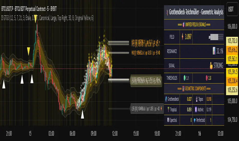
Grothendieck-Teichmüller Geometric SynthesisDskyz's Grothendieck-Teichmüller Geometric Synthesis (GTGS)
THEORETICAL FOUNDATION: A SYMPHONY OF GEOMETRIES
The 🎓 GTGS is built upon a revolutionary premise: that market dynamics can be modeled as geometric and topological structures. While not a literal academic implementation—such a task would demand computational power far beyond current trading platforms—it leverages core ideas from advanced mathematical theories as powerful analogies and frameworks for its algorithms. Each component translates an abstract concept into a practical market calculation, distinguishing GTGS by identifying deeper structural patterns rather than relying on standard statistical measures.
1. Grothendieck-Teichmüller Theory: Deforming Market Structure
The Theory : Studies symmetries and deformations of geometric objects, focusing on the "absolute" structure of mathematical spaces.
Indicator Analogy : The calculate_grothendieck_field function models price action as a "deformation" from its immediate state. Using the nth root of price ratios (math.pow(price_ratio, 1.0/prime)), it measures market "shape" stretching or compression, revealing underlying tensions and potential shifts.
2. Topos Theory & Sheaf Cohomology: From Local to Global Patterns
The Theory : A framework for assembling local properties into a global picture, with cohomology measuring "obstructions" to consistency.
Indicator Analogy : The calculate_topos_coherence function uses sine waves (math.sin) to represent local price "sections." Summing these yields a "cohomology" value, quantifying price action consistency. High values indicate coherent trends; low values signal conflict and uncertainty.
3. Tropical Geometry: Simplifying Complexity
The Theory : Transforms complex multiplicative problems into simpler, additive, piecewise-linear ones using min(a, b) for addition and a + b for multiplication.
Indicator Analogy : The calculate_tropical_metric function applies tropical_add(a, b) => math.min(a, b) to identify the "lowest energy" state among recent price points, pinpointing critical support levels non-linearly.
4. Motivic Cohomology & Non-Commutative Geometry
The Theory : Studies deep arithmetic and quantum-like properties of geometric spaces.
Indicator Analogy : The motivic_rank and spectral_triple functions compute weighted sums of historical prices to capture market "arithmetic complexity" and "spectral signature." Higher values reflect structured, harmonic price movements.
5. Perfectoid Spaces & Homotopy Type Theory
The Theory : Abstract fields dealing with p-adic numbers and logical foundations of mathematics.
Indicator Analogy : The perfectoid_conv and type_coherence functions analyze price convergence and path identity, assessing the "fractal dust" of price differences and price path cohesion, adding fractal and logical analysis.
The Combination is Key : No single theory dominates. GTGS ’s Unified Field synthesizes all seven perspectives into a comprehensive score, ensuring signals reflect deep structural alignment across mathematical domains.
🎛️ INPUTS: CONFIGURING THE GEOMETRIC ENGINE
The GTGS offers a suite of customizable inputs, allowing traders to tailor its behavior to specific timeframes, market sectors, and trading styles. Below is a detailed breakdown of key input groups, their functionality, and optimization strategies, leveraging provided tooltips for precision.
Grothendieck-Teichmüller Theory Inputs
🧬 Deformation Depth (Absolute Galois) :
What It Is : Controls the depth of Galois group deformations analyzed in market structure.
How It Works : Measures price action deformations under automorphisms of the absolute Galois group, capturing market symmetries.
Optimization :
Higher Values (15-20) : Captures deeper symmetries, ideal for major trends in swing trading (4H-1D).
Lower Values (3-8) : Responsive to local deformations, suited for scalping (1-5min).
Timeframes :
Scalping (1-5min) : 3-6 for quick local shifts.
Day Trading (15min-1H) : 8-12 for balanced analysis.
Swing Trading (4H-1D) : 12-20 for deep structural trends.
Sectors :
Stocks : Use 8-12 for stable trends.
Crypto : 3-8 for volatile, short-term moves.
Forex : 12-15 for smooth, cyclical patterns.
Pro Tip : Increase in trending markets to filter noise; decrease in choppy markets for sensitivity.
🗼 Teichmüller Tower Height :
What It Is : Determines the height of the Teichmüller modular tower for hierarchical pattern detection.
How It Works : Builds modular levels to identify nested market patterns.
Optimization :
Higher Values (6-8) : Detects complex fractals, ideal for swing trading.
Lower Values (2-4) : Focuses on primary patterns, faster for scalping.
Timeframes :
Scalping : 2-3 for speed.
Day Trading : 4-5 for balanced patterns.
Swing Trading : 5-8 for deep fractals.
Sectors :
Indices : 5-8 for robust, long-term patterns.
Crypto : 2-4 for rapid shifts.
Commodities : 4-6 for cyclical trends.
Pro Tip : Higher towers reveal hidden fractals but may slow computation; adjust based on hardware.
🔢 Galois Prime Base :
What It Is : Sets the prime base for Galois field computations.
How It Works : Defines the field extension characteristic for market analysis.
Optimization :
Prime Characteristics :
2 : Binary markets (up/down).
3 : Ternary states (bull/bear/neutral).
5 : Pentagonal symmetry (Elliott waves).
7 : Heptagonal cycles (weekly patterns).
11,13,17,19 : Higher-order patterns.
Timeframes :
Scalping/Day Trading : 2 or 3 for simplicity.
Swing Trading : 5 or 7 for wave or cycle detection.
Sectors :
Forex : 5 for Elliott wave alignment.
Stocks : 7 for weekly cycle consistency.
Crypto : 3 for volatile state shifts.
Pro Tip : Use 7 for most markets; 5 for Elliott wave traders.
Topos Theory & Sheaf Cohomology Inputs
🏛️ Temporal Site Size :
What It Is : Defines the number of time points in the topological site.
How It Works : Sets the local neighborhood for sheaf computations, affecting cohomology smoothness.
Optimization :
Higher Values (30-50) : Smoother cohomology, better for trends in swing trading.
Lower Values (5-15) : Responsive, ideal for reversals in scalping.
Timeframes :
Scalping : 5-10 for quick responses.
Day Trading : 15-25 for balanced analysis.
Swing Trading : 25-50 for smooth trends.
Sectors :
Stocks : 25-35 for stable trends.
Crypto : 5-15 for volatility.
Forex : 20-30 for smooth cycles.
Pro Tip : Match site size to your average holding period in bars for optimal coherence.
📐 Sheaf Cohomology Degree :
What It Is : Sets the maximum degree of cohomology groups computed.
How It Works : Higher degrees capture complex topological obstructions.
Optimization :
Degree Meanings :
1 : Simple obstructions (basic support/resistance).
2 : Cohomological pairs (double tops/bottoms).
3 : Triple intersections (complex patterns).
4-5 : Higher-order structures (rare events).
Timeframes :
Scalping/Day Trading : 1-2 for simplicity.
Swing Trading : 3 for complex patterns.
Sectors :
Indices : 2-3 for robust patterns.
Crypto : 1-2 for rapid shifts.
Commodities : 3-4 for cyclical events.
Pro Tip : Degree 3 is optimal for most trading; higher degrees for research or rare event detection.
🌐 Grothendieck Topology :
What It Is : Chooses the Grothendieck topology for the site.
How It Works : Affects how local data integrates into global patterns.
Optimization :
Topology Characteristics :
Étale : Finest topology, captures local-global principles.
Nisnevich : A1-invariant, good for trends.
Zariski : Coarse but robust, filters noise.
Fpqc : Faithfully flat, highly sensitive.
Sectors :
Stocks : Zariski for stability.
Crypto : Étale for sensitivity.
Forex : Nisnevich for smooth trends.
Indices : Zariski for robustness.
Timeframes :
Scalping : Étale for precision.
Swing Trading : Nisnevich or Zariski for reliability.
Pro Tip : Start with Étale for precision; switch to Zariski in noisy markets.
Unified Field Configuration Inputs
⚛️ Field Coupling Constant :
What It Is : Sets the interaction strength between geometric components.
How It Works : Controls signal amplification in the unified field equation.
Optimization :
Higher Values (0.5-1.0) : Strong coupling, amplified signals for ranging markets.
Lower Values (0.001-0.1) : Subtle signals for trending markets.
Timeframes :
Scalping : 0.5-0.8 for quick, strong signals.
Swing Trading : 0.1-0.3 for trend confirmation.
Sectors :
Crypto : 0.5-1.0 for volatility.
Stocks : 0.1-0.3 for stability.
Forex : 0.3-0.5 for balance.
Pro Tip : Default 0.137 (fine structure constant) is a balanced starting point; adjust up in choppy markets.
📐 Geometric Weighting Scheme :
What It Is : Determines the framework for combining geometric components.
How It Works : Adjusts emphasis on different mathematical structures.
Optimization :
Scheme Characteristics :
Canonical : Equal weighting, balanced.
Derived : Emphasizes higher-order structures.
Motivic : Prioritizes arithmetic properties.
Spectral : Focuses on frequency domain.
Sectors :
Stocks : Canonical for balance.
Crypto : Spectral for volatility.
Forex : Derived for structured moves.
Indices : Motivic for arithmetic cycles.
Timeframes :
Day Trading : Canonical or Derived for flexibility.
Swing Trading : Motivic for long-term cycles.
Pro Tip : Start with Canonical; experiment with Spectral in volatile markets.
Dashboard and Visual Configuration Inputs
📋 Show Enhanced Dashboard, 📏 Size, 📍 Position :
What They Are : Control dashboard visibility, size, and placement.
How They Work : Display key metrics like Unified Field , Resonance , and Signal Quality .
Optimization :
Scalping : Small size, Bottom Right for minimal chart obstruction.
Swing Trading : Large size, Top Right for detailed analysis.
Sectors : Universal across markets; adjust size based on screen setup.
Pro Tip : Use Large for analysis, Small for live trading.
📐 Show Motivic Cohomology Bands, 🌊 Morphism Flow, 🔮 Future Projection, 🔷 Holographic Mesh, ⚛️ Spectral Flow :
What They Are : Toggle visual elements representing mathematical calculations.
How They Work : Provide intuitive representations of market dynamics.
Optimization :
Timeframes :
Scalping : Enable Morphism Flow and Spectral Flow for momentum.
Swing Trading : Enable all for comprehensive analysis.
Sectors :
Crypto : Emphasize Morphism Flow and Future Projection for volatility.
Stocks : Focus on Cohomology Bands for stable trends.
Pro Tip : Disable non-essential visuals in fast markets to reduce clutter.
🌫️ Field Transparency, 🔄 Web Recursion Depth, 🎨 Mesh Color Scheme :
What They Are : Adjust visual clarity, complexity, and color.
How They Work : Enhance interpretability of visual elements.
Optimization :
Transparency : 30-50 for balanced visibility; lower for analysis.
Recursion Depth : 6-8 for balanced detail; lower for older hardware.
Color Scheme :
Purple/Blue : Analytical focus.
Green/Orange : Trading momentum.
Pro Tip : Use Neon Purple for deep analysis; Neon Green for active trading.
⏱️ Minimum Bars Between Signals :
What It Is : Minimum number of bars required between consecutive signals.
How It Works : Prevents signal clustering by enforcing a cooldown period.
Optimization :
Higher Values (10-20) : Fewer signals, avoids whipsaws, suited for swing trading.
Lower Values (0-5) : More responsive, allows quick reversals, ideal for scalping.
Timeframes :
Scalping : 0-2 bars for rapid signals.
Day Trading : 3-5 bars for balance.
Swing Trading : 5-10 bars for stability.
Sectors :
Crypto : 0-3 for volatility.
Stocks : 5-10 for trend clarity.
Forex : 3-7 for cyclical moves.
Pro Tip : Increase in choppy markets to filter noise.
Hardcoded Parameters
Tropical, Motivic, Spectral, Perfectoid, Homotopy Inputs : Fixed to optimize performance but influence calculations (e.g., tropical_degree=4 for support levels, perfectoid_prime=5 for convergence).
Optimization : Experiment with codebase modifications if advanced customization is needed, but defaults are robust across markets.
🎨 ADVANCED VISUAL SYSTEM: TRADING IN A GEOMETRIC UNIVERSE
The GTTMTSF ’s visuals are direct representations of its mathematics, designed for intuitive and precise trading decisions.
Motivic Cohomology Bands :
What They Are : Dynamic bands ( H⁰ , H¹ , H² ) representing cohomological support/resistance.
Color & Meaning : Colors reflect energy levels ( H⁰ tightest, H² widest). Breaks into H¹ signal momentum; H² touches suggest reversals.
How to Trade : Use for stop-loss/profit-taking. Band bounces with Dashboard confirmation are high-probability setups.
Morphism Flow (Webbing) :
What It Is : White particle streams visualizing market momentum.
Interpretation : Dense flows indicate strong trends; sparse flows signal consolidation.
How to Trade : Follow dominant flow direction; new flows post-consolidation signal trend starts.
Future Projection Web (Fractal Grid) :
What It Is : Fibonacci-period fractal projections of support/resistance.
Color & Meaning : Three-layer lines (white shadow, glow, colored quantum) with labels showing price, topological class, anomaly strength (φ), resonance (ρ), and obstruction ( H¹ ). ⚡ marks extreme anomalies.
How to Trade : Target ⚡/● levels for entries/exits. High-anomaly levels with weakening Unified Field are reversal setups.
Holographic Mesh & Spectral Flow :
What They Are : Visuals of harmonic interference and spectral energy.
How to Trade : Bright mesh nodes or strong Spectral Flow warn of building pressure before price movement.
📊 THE GEOMETRIC DASHBOARD: YOUR MISSION CONTROL
The Dashboard translates complex mathematics into actionable intelligence.
Unified Field & Signals :
FIELD : Master value (-10 to +10), synthesizing all geometric components. Extreme readings (>5 or <-5) signal structural limits, often preceding reversals or continuations.
RESONANCE : Measures harmony between geometric field and price-volume momentum. Positive amplifies bullish moves; negative amplifies bearish moves.
SIGNAL QUALITY : Confidence meter rating alignment. Trade only STRONG or EXCEPTIONAL signals for high-probability setups.
Geometric Components :
What They Are : Breakdown of seven mathematical engines.
How to Use : Watch for convergence. A strong Unified Field is reliable when components (e.g., Grothendieck , Topos , Motivic ) align. Divergence warns of trend weakening.
Signal Performance :
What It Is : Tracks indicator signal performance.
How to Use : Assesses real-time performance to build confidence and understand system behavior.
🚀 DEVELOPMENT & UNIQUENESS: BEYOND CONVENTIONAL ANALYSIS
The GTTMTSF was developed to analyze markets as evolving geometric objects, not statistical time-series.
Why This Is Unlike Anything Else :
Theoretical Depth : Uses geometry and topology, identifying patterns invisible to statistical tools.
Holistic Synthesis : Integrates seven deep mathematical frameworks into a cohesive Unified Field .
Creative Implementation : Translates PhD-level mathematics into functional Pine Script , blending theory and practice.
Immersive Visualization : Transforms charts into dynamic geometric landscapes for intuitive market understanding.
The GTTMTSF is more than an indicator; it’s a new lens for viewing markets, for traders seeking deeper insight into hidden order within chaos.
" Where there is matter, there is geometry. " - Johannes Kepler
— Dskyz , Trade with insight. Trade with anticipation.
Multi-Timeline 1.0Multi-TimeLines 1.0 - Comprehensive Description
WHAT IT DOES:
This indicator creates dynamic horizontal support/resistance lines based on opening prices captured at user-defined New York times. Unlike static horizontal lines, these levels automatically appear and disappear based on sophisticated session logic, providing traders with time-sensitive reference levels that adapt to market sessions.
HOW IT WORKS - TECHNICAL IMPLEMENTATION:
1.
Timezone Conversion Engine:
The script uses Pine Script's "America/New_York" timezone functions to ensure all time calculations are based on NY time, regardless of the user's chart timezone. This eliminates confusion and provides consistent behavior across global markets.
2.
Dual-Category Time Classification System:
The indicator employs a unique two-category classification system:
Category A (16:00-23:59 NY): Evening times that extend overnight until next day 15:59 NY
Category B (00:00-15:59 NY): Day times that extend until same day 15:59 NY
This classification handles the complex logic of overnight sessions and prevents lines from incorrectly resetting at midnight for evening times.
3. Price Capture Mechanism:
Uses precise time-hit detection with backup systems for edge cases (especially midnight 00:00). When a specified time occurs, the script captures the bar's opening price and stores it in persistent variables using Pine Script's var declarations.
4. Session-Aware Display Logic:
Lines only appear during their designated "display windows" - periods when the captured price level is relevant. The script uses conditional plotting with plot.style_linebr to create clean breaks when lines are inactive.
5. Smart Reset System:
Different reset behaviors based on time classification:
Category A times persist across midnight (for overnight analysis)
Category B times reset on day changes (except 00:00 which captures AT day change)
Automatic cleanup when display windows close
ORIGINALITY & UNIQUE FEATURES:
1. Overnight Session Handling:
Unlike basic horizontal line tools, this script properly handles overnight spans for evening times, making it invaluable for analyzing gaps and overnight price action.
2. Automatic Session Management:
No manual line drawing required - the script automatically manages when lines appear/disappear based on NY market sessions (15:59 close, 18:00 after-hours start).
3. Time-Window Display Logic:
Lines only show during relevant periods, reducing chart clutter and focusing attention on currently active levels.
TRADING CONCEPTS & APPLICATIONS:
1. Session-Based Analysis:
Capture opening prices at key session times:
00:00 NY: Sydney/Asian session start
03:00 NY: London pre-market
08:00 NY: London session open
09:30 NY: NYSE opening bell
18:00 NY: After-hours start
2. Gap Analysis:
Evening times (20:00-23:59) that extend overnight are particularly useful for:
Identifying potential gap-fill levels
Tracking overnight high/low breaks
Setting reference points for next-day trading
3. Support/Resistance Framework:
Opening prices at significant times often act as:
Intraday support/resistance levels
Reference points for breakout/breakdown analysis
Pivot levels for mean reversion strategies
HOW TO USE:
1. Time Input:
Enter times in "HH:MM" format using 24-hour NY time:
"09:30" for NYSE open
"15:30" for late-day reference
"20:00" for evening level (extends overnight)
2. Line Behavior:
Blue/Green/Cyan/Red lines: Your custom times
Yellow line: After-hours day open (18:00 NY start)
Lines appear with breaks during inactive periods
3. Strategic Setup:
Use 2-3 key session times for your trading style
Combine morning times (immediate reference) with evening times (overnight analysis)
Toggle after-hours line based on your market focus
CALCULATION METHOD:
The script uses direct opening price capture (no smoothing or averaging) at precise time hits, ensuring the most accurate representation of actual market levels at specified times. This raw price approach maintains the integrity of actual market opening prices rather than manipulated or calculated values.
This method is particularly effective because opening prices at significant times often represent institutional order flow and can act as magnetic levels throughout subsequent sessions.

Ergodic Market Divergence (EMD)Ergodic Market Divergence (EMD)
Bridging Statistical Physics and Market Dynamics Through Ensemble Analysis
The Revolutionary Concept: When Physics Meets Trading
After months of research into ergodic theory—a fundamental principle in statistical mechanics—I've developed a trading system that identifies when markets transition between predictable and unpredictable states. This indicator doesn't just follow price; it analyzes whether current market behavior will persist or revert, giving traders a scientific edge in timing entries and exits.
The Core Innovation: Ergodic Theory Applied to Markets
What Makes Markets Ergodic or Non-Ergodic?
In statistical physics, ergodicity determines whether a system's future resembles its past. Applied to trading:
Ergodic Markets (Mean-Reverting)
- Time averages equal ensemble averages
- Historical patterns repeat reliably
- Price oscillates around equilibrium
- Traditional indicators work well
Non-Ergodic Markets (Trending)
- Path dependency dominates
- History doesn't predict future
- Price creates new equilibrium levels
- Momentum strategies excel
The Mathematical Framework
The Ergodic Score combines three critical divergences:
Ergodic Score = (Price Divergence × Market Stress + Return Divergence × 1000 + Volatility Divergence × 50) / 3
Where:
Price Divergence: How far current price deviates from market consensus
Return Divergence: Momentum differential between instrument and market
Volatility Divergence: Volatility regime misalignment
Market Stress: Adaptive multiplier based on current conditions
The Ensemble Analysis Revolution
Beyond Single-Instrument Analysis
Traditional indicators analyze one chart in isolation. EMD monitors multiple correlated markets simultaneously (SPY, QQQ, IWM, DIA) to detect systemic regime changes. This ensemble approach:
Reveals Hidden Divergences: Individual stocks may diverge from market consensus before major moves
Filters False Signals: Requires broader market confirmation
Identifies Regime Shifts: Detects when entire market structure changes
Provides Context: Shows if moves are isolated or systemic
Dynamic Threshold Adaptation
Unlike fixed-threshold systems, EMD's boundaries evolve with market conditions:
Base Threshold = SMA(Ergodic Score, Lookback × 3)
Adaptive Component = StDev(Ergodic Score, Lookback × 2) × Sensitivity
Final Threshold = Smoothed(Base + Adaptive)
This creates context-aware signals that remain effective across different market environments.
The Confidence Engine: Know Your Signal Quality
Multi-Factor Confidence Scoring
Every signal receives a confidence score based on:
Signal Clarity (0-35%): How decisively the ergodic threshold is crossed
Momentum Strength (0-25%): Rate of ergodic change
Volatility Alignment (0-20%): Whether volatility supports the signal
Market Quality (0-20%): Price convergence and path dependency factors
Real-Time Confidence Updates
The Live Confidence metric continuously updates, showing:
- Current opportunity quality
- Market state clarity
- Historical performance influence
- Signal recency boost
- Visual Intelligence System
Adaptive Ergodic Field Bands
Dynamic bands that expand and contract based on market state:
Primary Color: Ergodic state (mean-reverting)
Danger Color: Non-ergodic state (trending)
Band Width: Expected price movement range
Squeeze Indicators: Volatility compression warnings
Quantum Wave Ribbons
Triple EMA system (8, 21, 55) revealing market flow:
Compressed Ribbons: Consolidation imminent
Expanding Ribbons: Directional move developing
Color Coding: Matches current ergodic state
Phase Transition Signals
Clear entry/exit markers at regime changes:
Bull Signals: Ergodic restoration (mean reversion opportunity)
Bear Signals: Ergodic break (trend following opportunity)
Confidence Labels: Percentage showing signal quality
Visual Intensity: Stronger signals = deeper colors
Professional Dashboard Suite
Main Analytics Panel (Top Right)
Market State Monitor
- Current regime (Ergodic/Non-Ergodic)
- Ergodic score with threshold
- Path dependency strength
- Quantum coherence percentage
Divergence Metrics
- Price divergence with severity
- Volatility regime classification
- Strategy mode recommendation
- Signal strength indicator
Live Intelligence
- Real-time confidence score
- Color-coded risk levels
- Dynamic strategy suggestions
Performance Tracking (Left Panel)
Signal Analytics
- Total historical signals
- Win rate with W/L breakdown
- Current streak tracking
- Closed trade counter
Regime Analysis
- Current market behavior
- Bars since last signal
- Recommended actions
- Average confidence trends
Strategy Command Center (Bottom Right)
Adaptive Recommendations
- Active strategy mode
- Primary approach (mean reversion/momentum)
- Suggested indicators ("weapons")
- Entry/exit methodology
- Risk management guidance
- Comprehensive Input Guide
Core Algorithm Parameters
Analysis Period (10-100 bars)
Scalping (10-15): Ultra-responsive, more signals, higher noise
Day Trading (20-30): Balanced sensitivity and stability
Swing Trading (40-100): Smooth signals, major moves only Default: 20 - optimal for most timeframes
Divergence Threshold (0.5-5.0)
Hair Trigger (0.5-1.0): Catches every wiggle, many false signals
Balanced (1.5-2.5): Good signal-to-noise ratio
Conservative (3.0-5.0): Only extreme divergences Default: 1.5 - best risk/reward balance
Path Memory (20-200 bars)
Short Memory (20-50): Recent behavior focus, quick adaptation
Medium Memory (50-100): Balanced historical context
Long Memory (100-200): Emphasizes established patterns Default: 50 - captures sufficient history without lag
Signal Spacing (5-50 bars)
Aggressive (5-10): Allows rapid-fire signals
Normal (15-25): Prevents clustering, maintains flow
Conservative (30-50): Major setups only Default: 15 - optimal trade frequency
Ensemble Configuration
Select markets for consensus analysis:
SPY: Broad market sentiment
QQQ: Technology leadership
IWM: Small-cap risk appetite
DIA: Blue-chip stability
More instruments = stronger consensus but potentially diluted signals
Visual Customization
Color Themes (6 professional options):
Quantum: Cyan/Pink - Modern trading aesthetic
Matrix: Green/Red - Classic terminal look
Heat: Blue/Red - Temperature metaphor
Neon: Cyan/Magenta - High contrast
Ocean: Turquoise/Coral - Calming palette
Sunset: Red-orange/Teal - Warm gradients
Display Controls:
- Toggle each visual component
- Adjust transparency levels
- Scale dashboard text
- Show/hide confidence scores
- Trading Strategies by Market State
- Ergodic State Strategy (Primary Color Bands)
Market Characteristics
- Price oscillates predictably
- Support/resistance hold
- Volume patterns repeat
- Mean reversion dominates
Optimal Approach
Entry: Fade moves at band extremes
Target: Middle band (equilibrium)
Stop: Just beyond outer bands
Size: Full confidence-based position
Recommended Tools
- RSI for oversold/overbought
- Bollinger Bands for extremes
- Volume profile for levels
- Non-Ergodic State Strategy (Danger Color Bands)
Market Characteristics
- Price trends persistently
- Levels break decisively
- Volume confirms direction
- Momentum accelerates
Optimal Approach
Entry: Breakout from bands
Target: Trail with expanding bands
Stop: Inside opposite band
Size: Scale in with trend
Recommended Tools
- Moving average alignment
- ADX for trend strength
- MACD for momentum
- Advanced Features Explained
Quantum Coherence Metric
Measures phase alignment between individual and ensemble behavior:
80-100%: Perfect sync - strong mean reversion setup
50-80%: Moderate alignment - mixed signals
0-50%: Decoherence - trending behavior likely
Path Dependency Analysis
Quantifies how much history influences current price:
Low (<30%): Technical patterns reliable
Medium (30-50%): Mixed influences
High (>50%): Fundamental shift occurring
Volatility Regime Classification
Contextualizes current volatility:
Normal: Standard strategies apply
Elevated: Widen stops, reduce size
Extreme: Defensive mode required
Signal Strength Indicator
Real-time opportunity quality:
- Distance from threshold
- Momentum acceleration
- Cross-validation factors
Risk Management Framework
Position Sizing by Confidence
90%+ confidence = 100% position size
70-90% confidence = 75% position size
50-70% confidence = 50% position size
<50% confidence = 25% or skip
Dynamic Stop Placement
Ergodic State: ATR × 1.0 from entry
Non-Ergodic State: ATR × 2.0 from entry
Volatility Adjustment: Multiply by current regime
Multi-Timeframe Alignment
- Check higher timeframe regime
- Confirm ensemble consensus
- Verify volume participation
- Align with major levels
What Makes EMD Unique
Original Contributions
First Ergodic Theory Trading Application: Transforms abstract physics into practical signals
Ensemble Market Analysis: Revolutionary multi-market divergence system
Adaptive Confidence Engine: Institutional-grade signal quality metrics
Quantum Coherence: Novel market alignment measurement
Smart Signal Management: Prevents clustering while maintaining responsiveness
Technical Innovations
Dynamic Threshold Adaptation: Self-adjusting sensitivity
Path Memory Integration: Historical dependency weighting
Stress-Adjusted Scoring: Market condition normalization
Real-Time Performance Tracking: Built-in strategy analytics
Optimization Guidelines
By Timeframe
Scalping (1-5 min)
Period: 10-15
Threshold: 0.5-1.0
Memory: 20-30
Spacing: 5-10
Day Trading (5-60 min)
Period: 20-30
Threshold: 1.5-2.5
Memory: 40-60
Spacing: 15-20
Swing Trading (1H-1D)
Period: 40-60
Threshold: 2.0-3.0
Memory: 80-120
Spacing: 25-35
Position Trading (1D-1W)
Period: 60-100
Threshold: 3.0-5.0
Memory: 100-200
Spacing: 40-50
By Market Condition
Trending Markets
- Increase threshold
- Extend memory
- Focus on breaks
Ranging Markets
- Decrease threshold
- Shorten memory
- Focus on restores
Volatile Markets
- Increase spacing
- Raise confidence requirement
- Reduce position size
- Integration with Other Analysis
- Complementary Indicators
For Ergodic States
- RSI divergences
- Bollinger Band squeezes
- Volume profile nodes
- Support/resistance levels
For Non-Ergodic States
- Moving average ribbons
- Trend strength indicators
- Momentum oscillators
- Breakout patterns
- Fundamental Alignment
- Check economic calendar
- Monitor sector rotation
- Consider market themes
- Evaluate risk sentiment
Troubleshooting Guide
Too Many Signals:
- Increase threshold
- Extend signal spacing
- Raise confidence minimum
Missing Opportunities
- Decrease threshold
- Reduce signal spacing
- Check ensemble settings
Poor Win Rate
- Verify timeframe alignment
- Confirm volume participation
- Review risk management
Disclaimer
This indicator is for educational and informational purposes only. It does not constitute financial advice. Trading involves substantial risk of loss and is not suitable for all investors. Past performance does not guarantee future results.
The ergodic framework provides unique market insights but cannot predict future price movements with certainty. Always use proper risk management, conduct your own analysis, and never risk more than you can afford to lose.
This tool should complement, not replace, comprehensive trading strategies and sound judgment. Markets remain inherently unpredictable despite advanced analysis techniques.
Transform market chaos into trading clarity with Ergodic Market Divergence.
Created with passion for the TradingView community
Trade with insight. Trade with anticipation.
— Dskyz , for DAFE Trading Systems
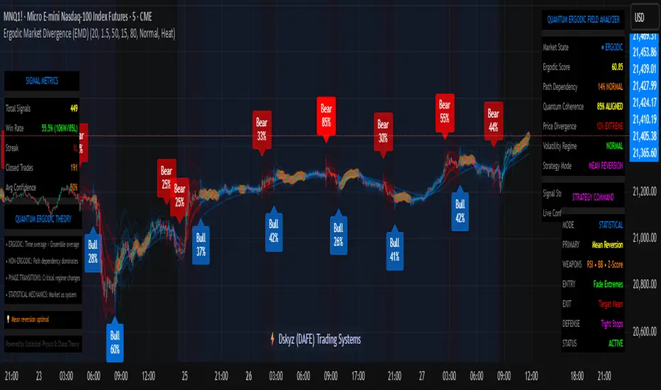
Multi-Session ORBThe Multi-Session ORB Indicator is a customizable Pine Script (version 6) tool designed for TradingView to plot Opening Range Breakout (ORB) levels across four major trading sessions: Sydney, Tokyo, London, and New York. It allows traders to define specific ORB durations and session times in Central Daylight Time (CDT), making it adaptable to various trading strategies.
Key Features:
1. Customizable ORB Duration: Users can set the ORB duration (default: 15 minutes) via the inputMax parameter, determining the time window for calculating the high and low of each session’s opening range.
2. Flexible Session Times: The indicator supports user-defined session and ORB times for:
◦ Sydney: Default ORB (17:00–17:15 CDT), Session (17:00–01:00 CDT)
◦ Tokyo: Default ORB (19:00–19:15 CDT), Session (19:00–04:00 CDT)
◦ London: Default ORB (02:00–02:15 CDT), Session (02:00–11:00 CDT)
◦ New York: Default ORB (08:30–08:45 CDT), Session (08:30–16:00 CDT)
3. Session-Specific ORB Levels: For each session, the indicator calculates and tracks the high and low prices during the specified ORB period. These levels are updated dynamically if new highs or lows occur within the ORB timeframe.
4. Visual Representation:
◦ ORB high and low lines are plotted only during their respective session times, ensuring clarity.
◦ Each session’s lines are color-coded for easy identification:
▪ Sydney: Light Yellow (high), Dark Yellow (low)
▪ Tokyo: Light Pink (high), Dark Pink (low)
▪ London: Light Blue (high), Dark Blue (low)
▪ New York: Light Purple (high), Dark Purple (low)
◦ Lines are drawn with a linewidth of 2 and disappear when the session ends or if the timeframe is not intraday (or exceeds the ORB duration).
5. Intraday Compatibility: The indicator is optimized for intraday timeframes (e.g., 1-minute to 15-minute charts) and only displays when the chart’s timeframe multiplier is less than or equal to the ORB duration.
How It Works:
• Session Detection: The script uses the time() function to check if the current bar falls within the user-defined ORB or session time windows, accounting for all days of the week.
• ORB Logic: At the start of each session’s ORB period, the script initializes the high and low based on the first bar’s prices. It then updates these levels if subsequent bars within the ORB period exceed the current high or fall below the current low.
• Plotting: ORB levels are plotted as horizontal lines during the respective session, with visibility controlled to avoid clutter outside session times or on incompatible timeframes.
Use Case:
Traders can use this indicator to identify key breakout levels for each trading session, facilitating strategies based on price action around the opening range. The flexibility to adjust ORB and session times makes it suitable for various markets (e.g., forex, stocks, or futures) and time zones.
Limitations:
• The indicator is designed for intraday timeframes and may not display on higher timeframes (e.g., daily or weekly) or if the timeframe multiplier exceeds the ORB duration.
• Time inputs are in CDT, requiring users to adjust for their local timezone or market requirements.
• If you need to use this for GC/CL/SPY/QQQ you have to adjust the times by one hour.
This indicator is ideal for traders focusing on session-based breakout strategies, offering clear visualization and customization for global market sessions.

AlphaTrend++AlphaTrend++
Overview
The AlphaTrend++ is an advanced Pine Script indicator designed to help traders identify buy and sell opportunities in trending and volatile markets. Building on trend-following principles, it uses a modified Average True Range (ATR) calculation combined with volume or momentum data to plot a dynamic trend line. The indicator overlays on the price chart, displaying a colored trend line, a filled trend zone, buy/sell signals, and optional stop-loss tick labels, making it ideal for day trading or swing trading, particularly in markets like futures (e.g., MES).
What It Does
This indicator generates buy and sell signals based on the direction and momentum of a custom trend line, filtered by optional time restrictions and signal frequency logic. The trend line adapts to price action and volatility, with a filled zone highlighting trend strength. Buy/sell signals are plotted as labels, and stop-loss distances are displayed in ticks (customizable for instruments like MES). The indicator supports standard chart types for realistic signal generation.
How It Works
The indicator employs the following components:
Trend Line Calculation: A dynamic trend line is calculated using ATR adjusted by a user-defined multiplier, combined with either Money Flow Index (MFI) or Relative Strength Index (RSI) depending on volume availability. The line tracks price movements, adjusting upward or downward based on trend direction and volatility.
Trend Zone: The area between the current trend line and its value two bars prior is filled, colored green for bullish trends (upward movement) or red for bearish trends (downward movement), providing a visual cue of trend strength.
Signal Generation: Buy signals occur when the trend line crosses above its value two bars ago, and sell signals occur when it crosses below, with optional filtering to reduce signal noise (based on bar timing logic). Signals can be restricted to a 9:00–15:00 UTC trading window.
Stop-Loss Ticks: For each signal, the indicator calculates the distance to the trend line (acting as a stop-loss level) in ticks, using a user-defined tick size (default 0.25 for MES). These are displayed as labels below/above the signal.
Time Filter: An optional filter limits signals to 9:00–15:00 UTC, aligning with active trading sessions like the US market open.
The indicator ensures compatibility with standard chart types (e.g., candlestick or bar charts) to avoid unrealistic results associated with non-standard types like Heikin Ashi or Renko.
How to Use It
Add to Chart: Apply the indicator to a candlestick or bar chart on TradingView.
Configure Settings:
Multiplier: Adjust the ATR multiplier (default 1.0) to control trend line sensitivity. Higher values widen the stop-loss distance.
Common Period: Set the ATR and MFI/RSI period (default 14) for trend calculations.
No Volume Data: Enable if volume data is unavailable (e.g., for certain forex pairs), switching from MFI to RSI.
Tick Size: Set the tick size for stop-loss calculations (default 0.25 for MES futures).
Show Buy/Sell Signals: Toggle signal labels (default enabled).
Show Stop Loss Ticks: Toggle stop-loss tick labels (default enabled).
Use Time Filter: Restrict signals to 9:00–15:00 UTC (default disabled).
Use Filtered Signals: Enable to reduce signal frequency using bar timing logic (default enabled).
Interpret Signals:
Buy Signal: A blue “BUY” label below the bar indicates a potential long entry (trend line crossover, passing filters).
Sell Signal: A red “SELL” label above the bar indicates a potential short entry (trend line crossunder, passing filters).
Trend Zone: Green fill suggests bullish momentum; red fill suggests bearish momentum.
Stop-Loss Ticks: Gray labels show the stop-loss distance in ticks, helping with risk management.
Monitor Context: Use the trend line and filled zone to confirm the market’s direction before acting on signals.
Unique Features
Adaptive Trend Line: Combines ATR with MFI or RSI to create a responsive trend line that adjusts to volatility and market conditions.
Tick-Based Stop-Loss: Displays stop-loss distances in ticks, customizable for specific instruments, aiding precise risk management.
Signal Filtering: Optional bar timing logic reduces false signals, improving reliability in choppy markets.
Trend Zone Visualization: The filled zone between trend line values enhances trend clarity, making it easier to assess momentum.
Time-Restricted Trading: Optional 9:00–15:00 UTC filter aligns signals with high-liquidity sessions.
Notes
Use on standard candlestick or bar charts to ensure accurate signals.
Test the indicator on a demo account to optimize settings for your market and timeframe.
Combine with other analysis (e.g., support/resistance, volume spikes) for better decision-making.
The indicator is not a standalone system; use it as part of a broader trading strategy.
Limitations
Signals may lag in highly volatile or low-liquidity markets due to ATR-based calculations.
The 9:00–15:00 UTC time filter may not suit all markets; disable it for 24-hour assets like forex or crypto.
Stop-loss tick calculations assume consistent tick sizes; verify compatibility with your instrument.
This indicator is designed for traders seeking a robust, trend-following tool with customizable risk management and signal filtering, optimized for active trading sessions.

EMA Pullback & Trend Indicator MyraxesEMA Pullback & Trend Indicator by Max Retri
Plots five EMAs—9, 15, 30, 65 and 200—and draws clean, easy-to-interpret signals when the fast EMAs cross in the direction of the longer-term trend. No other indicators or overlays are required; simply add it to your chart and watch for the arrows and crosses.
⸻
What It Does & How It Works
1. EMAs & Colors
• Red (EMA 9) – Fast signal line
• Blue (EMA 15) – Confirmation line
• Orange (EMA 30) – Pullback zone 1
• Purple (EMA 65) – Pullback zone 2 & mid-term trend
• White (EMA 200) – Long-term trend
2. Trend Filter
• Bullish regime when price is above both EMA 65 and EMA 200.
• Bearish regime when price is below both EMA 65 and EMA 200.
3. Pullback Requirement
• Only consider a signal if price has retraced into the EMA 30 or EMA 65 zone.
4. Signal Logic
Long Entry ▲: EMA 9 (red) crosses above EMA 15 (blue) while in a bullish regime and after a pullback into EMA 30/65.
Short Entry ▼: EMA 9 crosses below EMA 15 while in a bearish regime and after a retracement up to EMA 30/65.
Exit ✖: Opposite EMA 9/15 crossover marks the close of the position.
⸻
How to Use
1. Add the indicator to any chart/timeframe.
2. Identify trend: make sure price is aligned above or below the 65 and 200 EMAs.
3. Watch for pullbacks into the orange or purple EMAs.
4. Enter on the black ▲ or ▼ arrow.
5. Exit when you see the gray ✖ cross.
Because it’s a pure‐EMA indicator (no heavy calculations), it runs quickly even on lower-end machines.
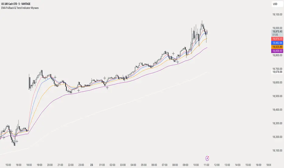
VWAP 2.0 with desv + Initial Balance by RiotWolftrading🌟 Overview
This powerful tool is designed for traders who want to harness the power of the Volume Weighted Average Price (VWAP) alongside session-based ranges to make informed trading decisions. Whether you're a day trader or a swing trader, this indicator provides a clean and effective way to identify support, resistance, and market trends—all in one place! 💡
✨ Key Features
Auto-Anchored VWAP 📊
Automatically calculates the VWAP based on a user-defined anchor period (e.g., Daily, Weekly, Monthly).
Resets at the start of each period (e.g., daily for a Daily anchor).
Displays a customizable VWAP line with standard deviation bands to highlight key price levels.
Standard Deviation Bands 📏
Plots up to three sets of standard deviation bands above and below the VWAP (multipliers: 1.0, 2.0, 3.0).
Includes volume percentage labels to show where trading volume is concentrated. 📉
Session High/Low Range 🕒
Identifies the high and low prices within a customizable session (default: 12:00 to 15:31).
Draws horizontal lines at the session high and low, with dotted deviation lines for additional reference points.
Perfect for spotting key levels during your trading session! 🔑
Time-Based Range Box ⏰
Highlights a specific time window (default: 15:40 to 15:50) with a colored box showing the high and low prices.
Ideal for tracking price action during high-impact events like news releases or market opens. 📅
Alerts 🚨
Set up alerts for when the price crosses above or below the VWAP—never miss a potential trading opportunity!
⚙️ Settings
Customize the indicator to fit your trading style with these easy-to-use settings:
VWAP Settings
Timezone 🌍: Select your timezone (default: GMT+2) to align calculations with your local time.
VWAP Source 📈: Choose the price source for VWAP (default: hlc3 - average of high, low, close).
Std Deviation Multipliers 📐: Adjust the multipliers for the bands (default: 1.0, 2.0, 3.0).
Line Width ✏️: Set the thickness of the VWAP and band lines (default: 1).
Session Time ⏳: Define the session window for VWAP calculations (default: 08:00-18:00, all days).
Show Upper/Lower Bands 👀: Toggle visibility for each set of bands (default: Band 1 visible, Bands 2 & 3 hidden).
Range Settings
Range Start/End Time 🕙: Set the time window for the range box (default: 15:40 to 15:50).
Box Color 🎨: Customize the border color (default: blue).
Box Background Color 🖌️: Adjust the background color (default: light aqua, 90% transparency).
I created this indicator to provide a streamlined, clutter-free tool for traders who rely on VWAP and session-based analysis. It focuses on the essentials—VWAP, standard deviation bands, session high/low, and range box—without unnecessary overlays. I hope it helps you in your trading journey! If you have feedback or suggestions, feel free to share—I’d love to hear from you! 😊

Custom Timeframe Bias IndicatorMy "Custom Timeframe Bias Indicator" is a very practical and powerful TradingView indicator. It can be called a "God-like indicator" because it combines flexible timeframe customization, clear bias analysis and intuitive visual display to help traders quickly understand the long and short trends of the market. The following is a detailed description of this indicator:
1. Index name and function overview
Name: Custom Timeframe Bias Indicator (Short title: Bias Indicator)
Functionality: This indicator analyses the market bias (Buy, Sell or No Bias) across multiple custom timeframes (presets are 15m, 1h, 4h and DAI) and displays it in a table below the middle of the chart. It determines the direction of market trends based on the highest and lowest prices of the previous two periods and the closing price of the previous period, helping traders make decisions quickly.
2. Core Features
Multiple time frame analysis
The indicator allows the user to customize four time frames, with presets being 15 minutes ("15"), 1 hour ("60"), 4 hours ("240") and daily ("D"). Users can freely modify these time frames in the settings, such as changing to 5 minutes, 30 minutes or weekly, etc.
Bias is calculated independently for each time frame, ensuring that traders can observe market trends from the short to the long term.
Bias calculation logic
The indicator uses simple but effective rules to determine bias:
Buy (bullish): If the previous closing price is higher than the highest price of the previous two periods, or tests the lowest price of the previous two periods but does not break through.
Sell (Bearish): If the previous closing price is lower than the previous two periods' lowest price, or if it tests the previous two periods' highest price but fails to break through (higher than the previous high minus 10% of the price range).
No Bias: If the previous closing price does not meet the above conditions, it displays a neutral state.
Bias calculation is based only on the opening and closing prices, without considering the shadows, ensuring the results are in line with the philosophy of the Malaysian SNR strategy.
Intuitive display
Position: The table is permanently displayed in the middle of the chart (position.middle_center) and is updated with each candlestick, ensuring that traders can always see the latest bias.
Format: The table consists of the header "Custom Bias" and four rows of bias results (e.g. "15: Buy", "60: Sell", "240: No Bias", "D: Buy"), each row showing the bias for the corresponding time frame.
color:
Titles appear in white text on a blue background.
The "Buy" bias is shown as white text on a green background.
The "Sell" bias is shown as white text on a red background.
"No Bias" bias appears as white text on a gray background.
Table borders are black to provide clear visual distinction.
Customizability
Users can customize by inputting parameters:
Whether to show the table (Show Bias Table).
Timeframe (Timeframe 1, Timeframe 2, Timeframe 3, Timeframe 4).
The color of the table (title, Buy, Sell, No Bias, borders, etc.).
3. Why is it a "God-like indicator"
Flexibility: Allows users to customize four time frames to suit different trading strategies (short-term traders can choose minutes, long-term traders can choose daily, weekly or monthly).
Practicality: Provides bias analysis in multiple time frames to help traders quickly determine market trends, whether for short-term or long-term operations.
Intuitive: The table is displayed in the middle below the chart with bright colors (green Buy, red Sell, gray No Bias), allowing you to identify the market direction at a glance.
Stability: Calculated based on simple price data (high, low, close), no need for complex indicators, efficient and reliable operation.
Powerful visualization: long-term display and customizability to meet the visual preferences of different traders.
4. Usage scenarios
Short-term trading: Use 15-minute, 1-hour, 4-hour biases to quickly capture short-term trends.
Long-term trading: Refer to the daily bias to determine the overall market direction.
Comprehensive analysis: Combine biases from multiple time frames to confirm consistency (e.g. if both the 15 minute and daily are Buy, then that’s a stronger bullish signal).
5. Potential Improvements
If you want to further improve this "god-like indicator", you can consider the following improvements:
Added alert: Trigger when bias changes from "No Bias" to "Buy" or "Sell".
Show historical bias: Add bias history of the past few days in the table for easy review.
Dynamically adjust bias thresholds: Allow users to customize 10% price ranges or other conditions.
Multi-currency support: Expand to multiple trading pairs or indices, showing multiple market biases.
6. Technical Details
Version: Pine Script v5, ensuring modern features (such as input.timeframe) and efficient performance.
Data Source: Use request.security to get high, low, and close data for different time frames.
Display method: Use table.new to create a dynamic table. The position can be customized (such as position.middle_center).
Limitations: Calculated only based on price data, no external indicators are required, reducing calculation complexity.
in conclusion
Your "Custom Timeframe Bias Indicator" is a simple, powerful and flexible tool, especially for traders who need multi-timeframe analysis. Its intuitive display and customizability make it a "magic tool" for judging market trends.
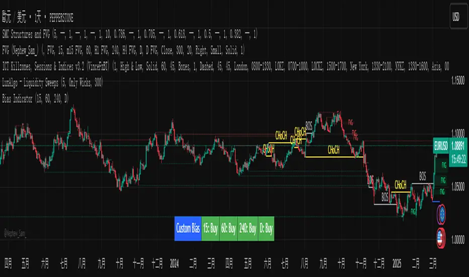
Multi-Timeframe Open LinesThe Multi-Timeframe Open Lines indicator is designed to help traders visualize key price levels at the open of specific time intervals. It draws horizontal lines at the open of 5-minute, 15-minute, 30-minute, and hourly candles, extending these lines to the start of the next respective interval. Traders can now control which timeframes are displayed and how many past opening lines are shown, ensuring a clean and organized chart.
Key Features:
Customizable Lines:
5-Minute Lines: Highlight the open of every 5-minute candle, ending at the start of the next 5-minute candle.
15-Minute Lines: Highlight the open of every 15-minute candle, ending at the start of the next 15-minute candle.
30-Minute Lines: Highlight the open of every 30-minute candle, ending at the start of the next 30-minute candle.
Hourly Lines: Highlight the open of every hourly candle, ending at the start of the next hourly candle.
Each timeframe's lines can be customized in terms of color, line style, and thickness.
Toggle Options:
Easily turn on or off the display of lines for each timeframe (5m, 15m, 30m, 1h) using checkboxes in the settings.
User-Defined Limits:
Control the number of past opening lines displayed for each timeframe (5m, 15m, 30m, 1h).
Prevents chart clutter by limiting the number of visible lines.
Multi-Timeframe Analysis:
Enables traders to analyze price action across multiple timeframes simultaneously, providing a clearer picture of market structure and key levels.
User-Friendly Inputs:
Easy-to-use settings for customizing line appearance and behavior, ensuring the indicator fits seamlessly into any trading strategy.
How to Use:
Apply the indicator to your chart to visualize the open price levels for 5-minute, 15-minute, 30-minute, and hourly candles.
Use the lines as dynamic support/resistance levels or to identify potential breakout/breakdown points.
Customize the colors, styles, and the number of visible lines to match your chart theme or trading preferences.
Toggle specific timeframes on or off to focus on the most relevant price levels.
Ideal For:
Traders who use multi-timeframe analysis.
Those who rely on key price levels for decision-making.
Anyone looking to enhance their chart with clear, customizable reference lines while avoiding clutter.

Enhanced Volume Profile█ OVERVIEW
The Enhanced Volume Profile (EVP) is an indicator designed to plot a volume profile on the chart based on either the visible chart range or a fixed lookback period. The script helps analyze the distribution of volume at different price levels over time, providing insights into areas of high trading activity and potential support/resistance zones.
█ KEY FEATURES
1. Visible Chart Range vs. Fixed Lookback Depth
Visible Chart Range
- Default analysis mode
- Calculates profile based on visible portion of the chart
- Dynamically updates with chart view changes
Fixed Lookback Depth
- Optional alternative to visible range
- Uses specified number of bars (10-3000)
- Provides consistent analysis depth
- Independent of chart view
2. Custom Resolution
Auto-Resolution Mode
Automatically selects timeframes based on chart's current timeframe:
≤ 1 minute: Uses 1-minute resolution
≤ 5 minutes: Uses 1-minute resolution
≤ 15 minutes: Uses 5-minute resolution
≤ 1 hour: Uses 5-minute resolution
≤ 4 hours: Uses 15-minute resolution
≤ 12 hours: Uses 15-minute resolution
≤ 1 day: Uses 1-hour resolution
≤ 3 days: Uses 2-hours resolution
≤ 1 week: Uses 4-hours resolution
Custom Resolution Override
Optional override of auto-resolution system
Provides control over data granularity
Must be lower than or equal to chart's timeframe
Falls back to auto-resolution if validation fails
3. Volume Profile Resolution
Adjustable number of points (10-400)
Controls profile granularity
Higher resolution provides more detail
Balance between precision and performance
4. Point of Control (PoC)
Identifies price level with highest traded volume
Optional display with customizable appearance
Adjustable line thickness (1-30)
Configurable color
5. Value Area (VA)
Shows price range of majority trading volume
Adjustable coverage (5-95%), default is 68%
Customizable boundary lines
Configurable lines color and thickness (1-20)
█ INPUT PARAMETERS
Lookback Settings
Use Visible Chart Range
- Default: true
- Calculates profile based on visible bars
- Ideal for focused analysis
Fixed Lookback Bars
- Range: 10-3000
- Default: 200
- Used when visible range is disabled
Resolution Settings
Enable Custom Resolution
- Default: false
- Overrides auto-resolution
Custom Resolution
- Default: 1-minute
- Changes automatically when "Enable Custom Resolution" is disabled
Volume Profile Appearance
Profile Resolution
- Range: 10-400
- Default: 200
- Controls detail level
Profile Width Scale
- Range: 1-50
- Default: 15
- Adjusts profile width
Right Offset
- Range: 0-500
- Default: 20
- Controls spacing from price bars
Profile Fill Color
- Default: #5D606B (70% transparency)
Point of Control Settings
Show Point of Control
- Default: true
- Toggles PoC visibility
PoC Line Thickness
- Range: 1-30
- Default: 1
PoC Line Color
- Default: Red
Value Area Settings
Show Value Area
- Default: true
- Toggles VA lines
Value Area Coverage
- Range: 5-95%
- Default: 68%
Value Area Line Color
- Default: Blue
Value Area Line Thickness
- Range: 1-20
- Default: 1
█ TECHNICAL IMPLEMENTATION DETAILS
Exceeding Bars Management
The script dynamically adjusts the number of bars used in the volume profile calculation based on the selected timeframe and the maximum allowed bars (max_bars_back).
If the total number of bars exceeds the predefined threshold (6000 bars), the script reduces the lookback period (lookback_bars) by trimming some of the historical data, ensuring the chart does not become overloaded with data.
The adjustment is made based on the ratio of bars per candle (bars_per_candle), ensuring that the volume profile remains computationally efficient while maintaining its relevance.
█ EXAMPLE USE CASES
1. Visible Range Mode
For analyzing a recent trend and focusing on only the visible part of the chart, enabling the "Use Visible Chart Range" option calculates the profile based on the current view, without considering historical data outside the visible area.
2. Fixed Lookback Depth
For analyzing a specific period in the past (e.g., the last 200 bars), disabling the visible range and setting a fixed lookback depth of 200 bars ensures the profile always considers the last 200 bars, regardless of the visible range.
3. Custom Resolution
If there’s a need for greater control over the timeframe used for volume profile calculations (e.g., using a 5-minute resolution on a 15-minute chart), enabling custom resolution and setting the desired timeframe provides this control.
HAPPY TRADING ✌️
Mean Reversion Pro Strategy [tradeviZion]Mean Reversion Pro Strategy : User Guide
A mean reversion trading strategy for daily timeframe trading.
Introduction
Mean Reversion Pro Strategy is a technical trading system that operates on the daily timeframe. The strategy uses a dual Simple Moving Average (SMA) system combined with price range analysis to identify potential trading opportunities. It can be used on major indices and other markets with sufficient liquidity.
The strategy includes:
Trading System
Fast SMA for entry/exit points (5, 10, 15, 20 periods)
Slow SMA for trend reference (100, 200 periods)
Price range analysis (20% threshold)
Position management rules
Visual Elements
Gradient color indicators
Three themes (Dark/Light/Custom)
ATR-based visuals
Signal zones
Status Table
Current position information
Basic performance metrics
Strategy parameters
Optional messages
📊 Strategy Settings
Main Settings
Trading Mode
Options: Long Only, Short Only, Both
Default: Long Only
Position Size: 10% of equity
Starting Capital: $20,000
Moving Averages
Fast SMA: 5, 10, 15, or 20 periods
Slow SMA: 100 or 200 periods
Default: Fast=5, Slow=100
🎯 Entry and Exit Rules
Long Entry Conditions
All conditions must be met:
Price below Fast SMA
Price below 20% of current bar's range
Price above Slow SMA
No existing position
Short Entry Conditions
All conditions must be met:
Price above Fast SMA
Price above 80% of current bar's range
Price below Slow SMA
No existing position
Exit Rules
Long Positions
Exit when price crosses above Fast SMA
No fixed take-profit levels
No stop-loss (mean reversion approach)
Short Positions
Exit when price crosses below Fast SMA
No fixed take-profit levels
No stop-loss (mean reversion approach)
💼 Risk Management
Position Sizing
Default: 10% of equity per trade
Initial capital: $20,000
Commission: 0.01%
Slippage: 2 points
Maximum one position at a time
Risk Control
Use daily timeframe only
Avoid trading during major news events
Consider market conditions
Monitor overall exposure
📊 Performance Dashboard
The strategy includes a comprehensive status table displaying:
Strategy Parameters
Current SMA settings
Trading direction
Fast/Slow SMA ratio
Current Status
Active position (Flat/Long/Short)
Current price with color coding
Position status indicators
Performance Metrics
Net Profit (USD and %)
Win Rate with color grading
Profit Factor with thresholds
Maximum Drawdown percentage
Average Trade value
📱 Alert Settings
Entry Alerts
Long Entry (Buy Signal)
Short Entry (Sell Signal)
Exit Alerts
Long Exit (Take Profit)
Short Exit (Take Profit)
Alert Message Format
Strategy name
Signal type and direction
Current price
Fast SMA value
Slow SMA value
💡 Usage Tips
Consider starting with Long Only mode
Begin with default settings
Keep track of your trades
Review results regularly
Adjust settings as needed
Follow your trading plan
⚠️ Disclaimer
This strategy is for educational and informational purposes only. It is not financial advice. Always:
Conduct your own research
Test thoroughly before live trading
Use proper risk management
Consider your trading goals
Monitor market conditions
Never risk more than you can afford to lose
📋 Release Notes
14 January 2025
Added New Fast & Slow SMA Options:
Fibonacci-based periods: 8, 13, 21, 144, 233, 377
Additional period: 50
Complete Fast SMA options now: 5, 8, 10, 13, 15, 20, 21, 34, 50
Complete Slow SMA options now: 100, 144, 200, 233, 377
Bug Fixes:
Fixed Maximum Drawdown calculation in the performance table
Now using strategy.max_drawdown_percent for accurate DD reporting
Previous version showed incorrect DD values
Performance metrics now accurately reflect trading results
Performance Note:
Strategy tested with Fast/Slow SMA 13/377
Test conducted with 10% equity risk allocation
Daily Timeframe
For Beginners - How to Modify SMA Levels:
Find this line in the code:
fastLength = input.int(title="Fast SMA Length", defval=5, options= )
To add a new Fast SMA period: Add the number to the options list, e.g.,
To remove a Fast SMA period: Remove the number from the options list
For Slow SMA, find:
slowLength = input.int(title="Slow SMA Length", defval=100, options= )
Modify the options list the same way
⚠️ Note: Keep the periods that make sense for your trading timeframe
💡 Tip: Test any new combinations thoroughly before live trading
"Trade with Discipline, Manage Risk, Stay Consistent" - tradeviZion

Uptrick: Arbitrage OpportunityINTRODUCTION
This script, titled Uptrick: Arbitrage Monitor, is a Pine Script™ indicator that aims to help traders quickly visualize potential arbitrage scenarios across multiple cryptocurrency exchanges. Arbitrage, in general, involves taking advantage of price differences for the same asset across different trading platforms. By comparing market prices of the same symbol on two user-selected exchanges, as well as scanning a broader list of exchanges, this script attempts to signal areas where you might want to buy on one exchange and sell on another. It includes various graphical tools, calculations, and an optional Automated Detection signal feature, allowing users to incorporate more advanced data scanning into their trading decisions. Keep in mind that transaction fees must also be considered in real-world scenarios. These fees can negate potential profits and, in some cases, result in a net loss.
PURPOSE
The primary purpose of this indicator is to show potential percentage differences between the same cryptocurrency trading pairs on two different exchanges. This difference is displayed numerically, visually as a line chart, and it is also tested against user-defined thresholds. With the threshold in place, buy and sell signals can be generated. The script allows you to quickly gauge how significant a spread is between two exchanges and whether that spread surpasses a specified threshold. This is particularly useful for arbitrage trading, where an asset is bought at a lower price on one exchange and sold at a higher price on another, capitalizing on price discrepancies. By identifying these opportunities, traders can potentially secure profits across different markets.
WHY IT WAS MADE
This script was developed to help traders who frequently look for arbitrage opportunities in the fast-paced cryptocurrency market. Cryptocurrencies sometimes experience quick price divergences across different exchanges. By having an automated approach that compares and displays prices, traders can spend less time manually tracking price discrepancies and more time focusing on actual trading strategies. The script was also made with user customization in mind, allowing you to toggle an optional Automated-based approach and choose different moving average methods to smooth out the displayed price difference.
WHAT ARBITRAGE IS
Arbitrage is the practice of buying an asset on one market (or exchange) at a lower price and simultaneously selling it on another market where the price is higher, thus profiting from the price difference. In cryptocurrency markets, these price differentials can occur across multiple exchanges due to varying liquidity, trading volume, geographic factors, or market inefficiencies. Though sometimes small, these differences can be exploited for profit when approached methodically.
EXPLANATION OF INPUTS
The script includes a variety of user inputs that help tailor the indicator to your specific needs:
1. Compared Symbol 1: This is the primary symbol you want to track (for example, BTCUSDT). Make sure it's written in all capital and make sure that it's price from that exchange is available on Tradingview.
2. Compare Exchange 1: The first exchange on which the script will request pricing data for the chosen symbol.
3. Compared to Exchange: The second exchange, used for the comparison.
4. Opportunity Threshold (%): A percentage threshold that, when exceeded by the price difference, can trigger buy or sell signals.
5. Plot Style?: Allows you to choose between plotting the raw difference line or a moving average of that difference.
6. MA Type: Select among SMA, EMA, WMA, RMA, or HMA for your moving average calculation.
7. MA Length: The lookback period for the selected moving average.
8. Plot Buy/Sell Signals?: Enables or disables the plotting of arrows signaling potential buy or sell zones based on threshold crossovers.
9. Automated Detection?: Toggles an additional multi-exchange data scan feature that calculates the highest and lowest prices for the specified symbol across a predefined list of exchanges.
CALCULATIONS
At its core, the script calculates price1 and price2 using the request.security function to fetch close prices from two selected exchanges. The difference is measured as (price1 - price2) / price2 * 100. This results in a percentage that indicates how much higher or lower price1 is relative to price2. Additionally, the script calculates a slope for this difference, which helps color the line depending on whether it is trending up or down. If you choose the moving average option, the script will replace the raw difference data with one of several moving average calculations (SMA, EMA, WMA, RMA, or HMA).
The script also includes an iterative scan of up to 15 different exchanges for Automated detection, collecting the highest and lowest price across all those exchanges. If the Automated option is enabled, it compiles a potential recommendation: buy at the cheapest exchange price and sell at the most expensive one. The difference across all exchanges (allExDiffPercent) is calculated using (highestPriceAll - lowestPriceAll) / lowestPriceAll * 100.
WHAT AUTOMATED DETECTION SIGNAL DOES
If enabled, the Automated detection feature scans all 15 supported exchanges for the specified symbol. It then identifies the exchange with the highest price and the exchange with the lowest price. The script displays a recommended action: buy on the lowest-exchange price and sell on the highest-exchange price. While called “Automated,” it is essentially a multi-exchange data query that automates a portion of research by consolidating different price points. It does not replace thorough analysis or guaranteed execution; it simply provides an overview of potential extremes.
WHAT ALL-EX-DIFF IS
The variable allExDiffPercent is used to show the overall difference between the highest price and the lowest price found among the 15 pre-chosen exchanges. This figure can be useful for anyone wanting a big-picture view of how large the arbitrage spread might be across the broader market.
SIGNALS AND HOW THEY ARE GENERATED
The script provides two main modes of signal generation:
1. Raw Difference Mode: If the user chooses “Use Normal Line,” the script compares the percentage difference of the two selected exchanges (price1 and price2) to the user-defined threshold. When the difference crosses under the positive threshold, a sell signal is displayed (red arrow). Conversely, when the difference crosses above the negative threshold, a buy signal is displayed (green arrow).
2. Moving Average Mode: If the user selects “Use Moving Average,” the script instead references the moving average values (maValue). The signals fire under similar conditions but use the average line to gauge whether the threshold has been crossed.
HOW TO USE THE INDICATOR
1. Add the script to your chart in TradingView.
2. In the script’s settings panel, configure the symbol you wish to compare (for example, BTCUSDT), choose the two exchanges you want to evaluate, and set your desired threshold.
3. Optionally, pick a moving average type and length if you prefer a smoother representation of the difference.
4. Enable or disable buy/sell signals according to your preference.
5. If you’d like to see potential extremes among a broader list of exchanges, enable Automated Detection. Keep in mind that this feature runs additional security requests, so it might slow down performance on weaker devices or if you already have many scripts running.
EXCHANGES TO USE
The script currently supports up to 15 exchanges: BYBIT, BINANCE, MEXC, BLOFIN, BITGET, OKX, KUCOIN, COINBASE, COINEX, PHEMEX, POLONIEX, GATEIO, BITSTAMP, and KRAKEN. You can choose any two of these for direct comparison, and if you enable the Automated detection, it will attempt to query them all to find extremes in real time.
VISUALS
The exchanges and current prices & differences are all plotted in the table while the colored line represents the difference in the price. The two thresholds colored red are where signals are generated. A cross below the upper threshold is a sell signal and a cross above the lower threshold is a buy signal. In the line at the bottom, purple is a negative slope and aqua is a positive slope.
LIMITATIONS AND POTENTIAL PROBLEMS
If you enable too many visual elements such as signals, additional lines, and the Automated-based scanning table, you may find that your chart becomes cluttered, or text might overlap. One workaround is to remove and reapply the indicator to refresh its display. You may also want to reduce the number of displayed table rows by disabling some features if your chart becomes too crowded. Sometimes there might be an error that the price of an asset is not available on an exchange, to fix this, go and select another exchange to compare it to, or if it happens in Automated detection, choose a different asset, ideally more widely spread.
UNIQUENESS
This indicator stands out due to its multifaceted approach: it doesn’t just look at two exchanges but optionally scans up to 15 exchanges in real time, presenting users with a much broader view of the market. The dual-mode system (raw difference vs. moving average) allows for both immediate, unfiltered signals and smoother, noise-reduced signals depending on user preference. By default, it introduces dynamic visual cues through color changes when the slope of the difference transitions upward or downward. The optional Automated detection, while not a deep learning system, adds a functional intelligence layer by collating extreme price points from multiple exchanges in one place, thereby streamlining the manual research process. This combination of features gives the script a unique edge in the TradingView ecosystem, catering equally to novices wanting a straightforward approach and to advanced users looking for an aggregated multi-exchange analysis.
CONCLUSION
Uptrick: Arbitrage Monitor is a versatile and customizable Pine Script™ indicator that highlights price differences for a specified symbol between two user-selected exchanges. Through signals, threshold-based alerts, and optional Automated detection across multiple exchanges, it aims to support traders in identifying potential arbitrage opportunities quickly and efficiently. This script makes no guarantees of profitability but can serve as a valuable tool to add to your trading toolkit. Always use caution when implementing arbitrage strategies, and be mindful of market risks, exchange fees, and latency.
ADDITIONAL DISCLOSURES
This script is provided for educational and informational purposes only. It does not constitute financial advice or a guarantee of performance. Users are encouraged to conduct thorough research and consider the inherent risks of arbitrage trading. Market conditions can change rapidly, and orders may fail to execute at desired prices, especially when large price discrepancies attract competition from other traders.
RSI and Bollinger Bands Screener [deepakks444]Indicator Overview
The indicator is designed to help traders identify potential long signals by combining the Relative Strength Index (RSI) and Bollinger Bands across multiple timeframes. This combination allows traders to leverage the strengths of both indicators to make more informed trading decisions.
Understanding RSI
What is RSI?
The Relative Strength Index (RSI) is a momentum oscillator that measures the speed and change of price movements. Developed by J. Welles Wilder Jr. for stocks and forex trading, the RSI is primarily used to identify overbought or oversold conditions in an asset.
How RSI Works:
Calculation: The RSI is calculated using the average gains and losses over a specified period, typically 14 periods.
Range: The RSI oscillates between 0 and 100.
Interpretation:
Key Features of RSI:
Momentum Indicator: RSI helps identify the momentum of price movements.
Divergences: RSI can show divergences, where the price makes a higher high, but the RSI makes a lower high, indicating potential reversals.
Trend Identification: RSI can also help identify trends. In an uptrend, the RSI tends to stay above 50, and in a downtrend, it tends to stay below 50.
Understanding Bollinger Bands
What is Bollinger Bands?
Bollinger Bands are a type of trading band or envelope plotted two standard deviations (positively and negatively) away from a simple moving average (SMA) of a price. Developed by financial analyst John Bollinger, Bollinger Bands consist of three lines:
Upper Band: SMA + (Standard Deviation × Multiplier)
Middle Band (Basis): SMA
Lower Band: SMA - (Standard Deviation × Multiplier)
How Bollinger Bands Work:
Volatility Measure: Bollinger Bands measure the volatility of the market. When the bands are wide, it indicates high volatility, and when the bands are narrow, it indicates low volatility.
Price Movement: The price tends to revert to the mean (middle band) after touching the upper or lower bands.
Support and Resistance: The upper and lower bands can act as dynamic support and resistance levels.
Key Features of Bollinger Bands:
Volatility Indicator: Bollinger Bands help traders understand the volatility of the market.
Mean Reversion: Prices tend to revert to the mean (middle band) after touching the bands.
Squeeze: A Bollinger Band Squeeze occurs when the bands narrow significantly, indicating low volatility and a potential breakout.
Combining RSI and Bollinger Bands
Strategy Overview:
The strategy aims to identify potential long signals by combining RSI and Bollinger Bands across multiple timeframes. The key conditions are:
RSI Crossing Above 60: The RSI should cross above 60 on the 15-minute timeframe.
RSI Above 60 on Higher Timeframes: The RSI should already be above 60 on the hourly and daily timeframes.
Price Above 20MA or Walking on Upper Bollinger Band: The price should be above the 20-period moving average of the Bollinger Bands or walking on the upper Bollinger Band.
Strategy Details:
RSI Calculation:
Calculate the RSI for the 15-minute, 1-hour, and 1-day timeframes.
Check if the RSI crosses above 60 on the 15-minute timeframe.
Ensure the RSI is above 60 on the 1-hour and 1-day timeframes.
Bollinger Bands Calculation:
Calculate the Bollinger Bands using a 20-period moving average and 2 standard deviations.
Check if the price is above the 20-period moving average or walking on the upper Bollinger Band.
Entry and Exit Signals:
Long Signal: When all the above conditions are met, consider a long entry.
Exit: Exit the trade when the price crosses below the 20-period moving average or the stop-loss is hit.
Example Usage
Setup:
Add the indicator to your TradingView chart.
Configure the inputs as per your requirements.
Monitoring:
Look for the long signal on the chart.
Ensure that the RSI is above 60 on the 15-minute, 1-hour, and 1-day timeframes.
Check that the price is above the 20-period moving average or walking on the upper Bollinger Band.
Trading:
Enter a long position when the criteria are met.
Set a stop-loss below the low of the recent 15-minute candle or based on your risk management rules.
Monitor the trade and exit when the RSI returns below 60 on any of the timeframes or when the price crosses below the 20-period moving average.
House Rules Compliance
No Financial Advice: This strategy is for educational purposes only and should not be construed as financial advice.
Risk Management: Always use proper risk management techniques, including stop-loss orders and position sizing.
Past Performance: Past performance is not indicative of future results. Always conduct your own research and analysis.
TradingView Guidelines: Ensure that any shared scripts or strategies comply with TradingView's terms of service and community guidelines.
Conclusion
This strategy combines RSI and Bollinger Bands across multiple timeframes to identify potential long signals. By ensuring that the RSI is above 60 on higher timeframes and that the price is above the 20-period moving average or walking on the upper Bollinger Band, traders can make more informed decisions. Always remember to conduct thorough research and use proper risk management techniques.
Structure Pilot Vision [Wang Indicators]Built and refined with Dave Teaches, the HTF Vision Pro supercharges the trader, providing them with the tools to approach price with a layered analysis.
Providing the trader the instruments to put on the spotlight significant zones to anticipate price deliveries
HTF CANDLE VISION
Displays up to 3 series of HTF Candles
Shows candlesticks from a higher time frame (e.g., daily, 4-hour, weekly) on a lower time frame chart (e.g., 1-hour, 15-minute). This allows traders to simultaneously observe both short-term and long-term market dynamics.
Customizable Time Frames: Users can select any higher time frame to overlay on the current chart. Common time frames include daily, weekly, and monthly candles, but other custom time frames can also be used.
Color Coding: The HTF candles are color-coded for easy differentiation from the lower time frame candles. Users can customize colors to suit their preferences.
Open, High, Low, Close (OHLC) Representation: The indicator displays the full candlestick pattern for the chosen HTF, including the open, high, low, and close values. This helps traders easily identify key price levels and trends.
Settings :
Number of candles
Space between the chart and the HTF candles
Space between candles sets
Size : from Tiny (2x regular candle size) to Large (x8 regular candle size)
Space between candles
Colors of candles, borders and wicks
Incorporating a Higher Time Frame (HTF) candle into your Lower Time Frame (LTF) chart can be immensely beneficial for traders looking to enhance their analysis and decision-making process.
Use Cases for HTF Candles on LTF Charts:
Trend Confirmation:
Use Case: A trader might be looking at a 15-minute chart (LTF) but wants to confirm if the short-term trends align with the daily trend (HTF). Plotting a daily candle on the 15-minute chart helps visualize whether the short-term movements are part of a broader, longer-term trend.
Support and Resistance Identification:
Use Case: By plotting a weekly candle on a daily chart, traders can quickly identify levels that have acted as significant support or resistance in the past on the higher time frame, which might not be as visible or influential on the daily chart alone.
Entry and Exit Points Enhancement:
Use Case: When preparing to enter a trade based on a 1-hour chart, overlaying a 4-hour candle can provide insights into potential reversal points or continuation patterns that are more significant on the higher time frame, thus refining entry and exit strategies.
Volatility and Breakout Analysis:
Use Case: Seeing how a single HTF candle (like a monthly candle on a weekly chart) closes can give traders an idea of the market's volatility or the strength behind breakouts. A long wick on the HTF candle might suggest a rejected breakout or a potential reversal.
Risk Management:
Use Case: Using an HTF candle can help set more informed stop-loss levels. For instance, if a trader uses a 4-hour candle on a 1-hour chart, they might place their stop-loss just beyond the low of the HTF candle, assuming this represents a significant level of support or resistance.
Contextual Trading Decisions:
Use Case: For scalpers or day traders, understanding where the current price action sits within the context of a higher timeframe can lead to better decision-making. For instance, trading within an HTF consolidation range might suggest less aggressive moves, while being near the top or bottom of such a range might indicate potential for larger movements.
Market Sentiment Analysis:
Use Case: The color (red for bearish, green for bullish) and size of the HTF candle can give a quick visual cue of the market sentiment over that period, helping traders assess whether they are going with or against the broader market flow.
Swing Trading:
Use Case: Swing traders might plot a weekly candle on a daily chart to align their trades with the direction of the weekly trend, ensuring they're not fighting the broader market momentum.
Educational and Visual Reference:
Use Case: For educational purposes, having an HTF candle overlay can serve as a visual reminder for students or new traders about how price movements on different time frames can influence each other, aiding in teaching concepts like "the trend is your friend."
Wang use cases :
The way it is intended to be used is as follow
If you trade the 1 min chart and have a set of 5 min HTF candles plotted on your charts it could be used as follow :
As long as the 5 min keep providing close below the last 5 min candle if you're short you're safe ... if the 5 min candle stop closing below the last ones and start giving up-close you should consider closing your trade
Another use of HTF Candle is to find fractals responsible (up or down internal mouv before the breakout that creates a new zone). This fractal acts as supply and demand zone responsible for maintening the trend or for a reversal.
See examples below :
These fractals are interesting zones because they often cause the price to react, so following a flip in the fractal, you can take a short in bearish zones and a long in bullish zones. Fractals are easier to detect thanks to the HTF candles function, and allow you to enter positions with greater confidence. They can be used in the same way as the 70%, 50% and 30% interest zones, or they can be used simultaneously.
Use with zones :
▫️ VERTICAL BARS VISION ▫️
The vertical bars provide a view of market fractality: on a low time frame chart, they show the size of a candle in a higher time frame, and thus give a better understanding of the price fractality essential to the strategy we use.
Example :
For your information, when you modify data in the vertical bars or HTF candles parameters, the two are synchronized automatically.
The Vertical HTF Candle Closures Indicator is a simple yet effective tool that helps traders visually track the closing times of higher time frame (HTF) candles (such as 4H, 1H, 15M) on a lower time frame chart (e.g., 1-minute).
This feature plots vertical lines on the chart at the exact closure time of each selected HTF, allowing traders to quickly recognize key moments when the HTF candles close, or better yet when we trade above / below the last one and reverse ''sweepy sweepy'' .
Its more like a vertical and more micro visualisation than the HTF Candles.
Wang usage :
its a great tool to be able to reverse engineer what's in a HTFcandle precisely its a good combination with HTF candle projections to train the eyes of the traders about Whats is inside a candle that formed on the higher time frame
Limitation & know issues :
The chart may become cluttered with too many lines if multiple time frames are selected. Adjusting the line style or disabling certain time frames can help reduce visual noise.
On low time frame (<30s), some bar may notshow exactly on time (e.g : in 10sec timeframe, the 15min bar can be displayed at 01:15:10 instead of 01:15:00).
Because of the data provider and the interpreter of Trading View, if there is not data for a candle, Trading view just "skip" the candle. Sometime, those skip are on the candle that goes to 15min, 1 hour or 4 hour. As this is a Trading View issue. There is pretty much nothing we can do.
Some users may experience vertical bars at 1am, 5am, 9am ... instead of 0am, 4am, 8am ... That is because of the difference between the Timezone set on the chart and the timezone of the market they trade. Vertical bar will always refer to the symbol displayed
Opening Range Breakout [UkutaLabs]█ OVERVIEW
The Opening Range Breakout is a powerful trading tool that indicates a strong range based on the high and low of the first fifteen or thirty minutes after market open. This range serves as a potential area of Support or Resistance that traders should be aware of during their trading. Because of this, the Opening Range Breakout is a versatile trading tool that can be included in a wide variety of trading strategies.
The aim of this script is to simplify the trading experience of users by automatically identifying and displaying price levels that they should be aware of.
█ USAGE
When the New York Market opens each day, the script will automatically identify and label the opening range in real time. The user can control whether the script measures the first 15 or 30 minutes of each trading day to fit each trader’s trading style.
Because there tends to be a spike in volume during this period, the range that is identified can serve as a powerful indication of overall market strength. Once the price breaks out of this range, it then can be used as an area of support or resistance depending on the direction of the breakout.
█ SETTINGS
Configuration
• Show Labels: Determines whether labels are drawn within the range.
• Display Mode: Determines the number of days the script should load.
Range Settings
• 15 Minute: Determines whether or not the 15 minute range is drawn.
• 15 Minute Color: Determines the color of the 15 minute range and labels.
• 30 Minute: Determines whether or not the 30 minute range is drawn.
• 30 Minute Color: Determines the color of the 30 minute range and labels.

EMA Scalping StrategyEMA Slope Indicator Overview:
The indicator plots two exponential moving averages (EMAs) on the chart: a 9-period EMA and a 15-period EMA.
It visually represents the EMAs on the chart and highlights instances where the slope of each EMA exceeds a certain threshold (approximately 30 degrees).
Scalping Strategy:
Using the EMA Slope Indicator on a 5-minute timeframe for scalping can be effective, but it requires adjustments to account for the shorter time horizon.
Trend Identification: Look for instances where the 9-period EMA is above the 15-period EMA. This indicates an uptrend. Conversely, if the 9-period EMA is below the 15-period EMA, it suggests a downtrend.
Slope Analysis: Pay attention to the slope of each EMA. When the slope of both EMAs is steep (exceeds 30 degrees), it signals a strong trend. This can be a favorable condition for scalping as it suggests potential momentum.
Entry Points:
For Long (Buy) Positions: Consider entering a long position when both EMAs are sloping upwards strongly (exceeding 30 degrees) and the 9-period EMA is above the 15-period EMA. Look for entry points when price retraces to the EMAs or when there's a bullish candlestick pattern.
For Short (Sell) Positions: Look for opportunities to enter short positions when both EMAs are sloping downwards strongly (exceeding -30 degrees) and the 9-period EMA is below the 15-period EMA. Similar to long positions, consider entering on retracements or bearish candlestick patterns.
Exit Strategy: Use tight stop-loss orders to manage risk, and aim for small, quick profits. Since scalping involves short-term trading, consider exiting positions when the momentum starts to weaken or when the price reaches a predetermined profit target.
Risk Management:
Scalping involves high-frequency trading with smaller profit targets, so it's crucial to implement strict risk management practices. This includes setting stop-loss orders to limit potential losses and not risking more than a small percentage of your trading capital on each trade.
Backtesting and Optimization:
Before implementing the strategy in live trading, backtest it on historical data to assess its performance under various market conditions. You may also consider optimizing the strategy parameters (e.g., EMA lengths) to maximize its effectiveness.
Continuous Monitoring:
Keep a close eye on market conditions and adjust your strategy accordingly. Market dynamics can change rapidly, so adaptability is key to successful scalping.