Ragi's 24h volumeThis script is a TradingView Pine Script indicator that displays the 24-hour trading volume for a given asset. It provides both the native volume of the asset and, if the asset is not already listed on Binance, also displays the 24-hour volume from Binance (if applicable). Here's a breakdown of the key components:
Volume Calculation:
It sums the volume data over different time frames: 1-minute, 5-minute (for daily charts), or 60-minute intervals.
The volume is calculated based on the asset's volume type (either "quote" volume or a calculated value of close * volume).
For crypto assets, if the volume data is unavailable, it raises an error.
Binance Volume:
If the asset is not from Binance, the script fetches 24-hour volume data from Binance for that symbol, ensuring it is using the correct currency rate.
Display:
The indicator displays a table with the 24-hour volume in the chosen position on the chart (top, middle, or bottom).
The table displays the current exchange's volume, and if applicable, the Binance volume.
The volume is color-coded based on predefined thresholds:
Attention: Displays a warning color for volumes exceeding the attention level.
Warning: Shows an alert color for volumes above the warning threshold.
Normal: Displays in standard color when the volume is lower than the warning level.
The text and background color are customizable, and users can adjust the text size and position of the table.
User Inputs:
The script allows customization of table text size, position, background color, and volume thresholds for attention and warning.
In summary, this indicator is designed to track and display 24-hour volume on a chart, with additional volume information from Binance if necessary, and provides visual cues based on volume levels to help traders quickly assess trading activity.
Cerca negli script per "豪24配债"
Timeframe-Based Dynamic MA [odnac]
This code is a Timeframe-Based Dynamic MA indicator, written in Pine Script, that dynamically calculates and displays the Simple Moving Average (SMA), Exponential Moving Average (EMA), and Volume Weighted Moving Average (VWMA) based on a 24-hour period, according to the selected timeframe. It automatically adjusts the length of the moving averages for each timeframe, showing the appropriate value optimized for that specific timeframe.
Code Explanation:
Settings:
inputLength: A user input that allows setting the base time (24 hours by default). This value determines the reference for calculating the length of the moving averages according to the timeframe.
transp: A setting for the transparency of the moving average lines. It can accept values from 0 to 100 (0 is opaque, 100 is fully transparent).
Timeframe-Based Moving Average Calculation:
The length variable is dynamically calculated based on the current chart's timeframe.
For shorter timeframes like 1-minute, 2-minute, 3-minute, 5-minute, 10-minute, 15-minute, 30-minute, and 45-minute, the length is calculated by multiplying 60 / selected timeframe to obtain the moving average length based on a 24-hour period.
For longer timeframes like 1 hour, 4 hours, and 1 day, fixed values are used to set the moving average length.
Moving Average Calculation:
sma, ema, vwma: These are the Simple Moving Average, Exponential Moving Average, and Volume Weighted Moving Average calculated based on the length.
else_sma, else_ema, else_vwma: These represent the moving averages fetched from the 1-hour chart. For timeframes that are not calculated directly, the values are taken from the 1-hour chart.
Displaying the Moving Averages:
The moving averages are plotted according to the length calculated for the current timeframe.
If the length for the current timeframe is valid, the corresponding SMA, EMA, and VWMA values are displayed. Otherwise, the values fetched from the 1-hour chart are used.
The moving averages are displayed with the transparency (transp) value set by the user, controlling their opacity on the chart.
How to Use:
Base Time: The user sets a base time. For example, setting inputLength to 24 will calculate the moving average length based on a 24-hour period, which will be dynamically adjusted and displayed according to the selected timeframe.
Transparency Setting: The transparency of the moving average lines can be adjusted using the transp value.
Supported Timeframes:
For shorter timeframes (1-minute, 2-minute, 3-minute, 5-minute, 10-minute, 15-minute, 30-minute, 45-minute), the moving average lengths are dynamically calculated and displayed.
For longer timeframes (1 hour, 4 hours, 1 day), fixed length values are used.
This indicator allows you to dynamically calculate daily moving averages across different timeframes and visually check which moving average is the most appropriate for the selected timeframe.

Ichimoku Kinko Hyo + HULL-MA_X + MacDThe Ichimoku Kinko Hyo system includes five kinds of signal, of which this strategy uses the most recent of ones i.e. Tenkan Sen / Kijun Sen Cross and price crosses the Kijun Sen. As the Chikou Span, Senkou Span A and Senkou Span B are shifted into the past/future, the trigger signals will be only be used for visual confirmation and not part of the strategy.
The Tenkan Sen, also known as the Turning or Conversion line, is a moving average of the highest high and lowest low over the last 9 periods in this strategy.
The Kijun Sen, also known as the Standard or Base line, is a moving average of the highest high and lowest low over the last 24 periods in this strategy.
The Chikou Span, also known as the Lagging line, is the closing price plotted 24 periods behind in this strategy.
The Senkou Span A, also known as the 1st leading line, is a moving average of the Tenkan Sen and Kijun Sen and is plotted 24 periods ahead in this strategy.
The Senkou Span B, also known as the 2nd leading line, is a moving average of the highest high and lowest low over the last 51 trading days is plotted 24 periods ahead in this strategy.
Moving average convergence divergence (MaCD) is a trend-following momentum indicator that shows the relationship between two moving averages of prices. The MaCD is calculated in this strategy by subtracting the 24-day exponential moving average (EMA) from the 12-day EMA. A nine-day EMA of the MACD, called the "signal line", aMaCD in this case, is then plotted on top of the MaCD. In this strategy, MaCD/ aMaCD Cross is functioning as a trigger for buy and sell signals.
As with most technical analysis methods, Ichimoku is likely to produce frequent conflicting signals in non-trending markets, So in addition to Ichimoku Kinko Hyo, the Hull MA is popular amongst some day traders, as the indicator which in combination with MaCD attempts to give an accurate signal by eliminating lags and improving the smoothness of the line.
Alan Hull, developed this moving average indicator and hence it’s called the Hull MA.
Now, let’s dissect how the Hull moving average is calculated.
The Hull MA involves the weighted moving average (WMA) in its calculation.
First, calculate the WMA with period (n / 2) and multiply this by 2. Remember ‘n’ is the time period configurable based on the trader’s requirement. The default setting is 12 periods in this strategy, fast Hull MA crossing slow Hull MA will generate a circle on charts.
Second, calculate the WMA for period “n” and subtract if from the first step. Thirdly, calculate the weighted moving average with period sqrt (n) using the data from the second step. You can take a look at the below formula:
Hull MA= WMA (2*WMA (n/2) − WMA (n)), sqrt (n))
The Hull MA Cross in combination with Tenkan Sen / Kijun Sen Cross and MaCD tries to give an accurate signal by eliminating lags and improve the smoothness of price activity. Please note that price trends can and do change often, so your readings of the charts and this trading system should be probabilistic, rather than predictive.

Mikula's Master 360° Square of 12Mikula’s Master 360° Square of 12
An educational W. D. Gann study indicator for price and time. Anchor a compact Square of 12 table to a start point you choose. Begin from a bar’s High or Low (or set a manual start price). From that anchor you can progress or regress the table to study how price steps through cycles in either direction.
What you’re looking at :
Zodiac rail (far left): the twelve signs.
Degree rail: 24 rows in 15° steps from 15° up to 360°/0°.
Transit rail and Natal rail: track one planet per rail. Each planet is placed at its current row (℞ shown when retrograde). As longitude advances, the planet climbs bottom → top, then wraps to the bottom at the next sign; during retrograde it steps downward.
Hover a planet’s cell to see a tooltip with its exact longitude and sign (e.g., 152.4° ♌︎). The linked price cell in the grid moves with the planet’s row so you can follow a planet’s path through the zodiac as a path through price.
Price grid (right): the 12×24 Square of 12. Each column is a cycle; cells are stepped price levels from your start price using your increment.
Bottom rail: shows the current square number and labels the twelve columns in that square.
How the square is read
The square always begins at the bottom left. Read each column bottom → top. At the top, return to the bottom of the next column and read up again. One square contains twelve cycles. Because the anchor can be a High or a Low, you can progress the table upward from the anchor or regress it downward while keeping the same bottom-to-top reading order.
Iterate Square (shifting)
Iterate Square shifts the entire 12×24 grid to the next set of twelve cycles.
Square 1 shows cycles 1–12; Square 2 shows 13–24; Square 3 shows 25–36, etc.
Visibility rules
Pivot cells are table-bound. If you shift the square beyond those prices, their highlights won’t appear in the table.
A/B levels and Transit/Natal planetary lines are chart overlays and can remain visible on the table as you shift the square.
Quick use
Choose an anchor (date/time + High/Low) or enable a manual start price .
Set the increment. If you anchored with a Low and want the table to step downward from there, use a negative value.
Optional: pick Transit and Natal planets (one per rail), toggle their plots, and hover their cells for longitude/sign.
Optional: turn on A/B levels to display repeating bands from the start price.
Optional: enable swing pivots to tint matching cells after the anchor.
Use Iterate Square to shift to later squares of twelve cycles.
Examples
These are exploratory examples to spark ideas:
Overview layout (zodiac & degree rails, Transit/Natal rails, price grid)
A-levels plotted, pivots tinted on the table, real-time price highlighted
Drawing angles from the anchor using price & time read from the table
Using a TradingView Gann box along the A-levels to study reactions
Attribution & originality
This script is an original implementation (no external code copied). Conceptual credit to Patrick Mikula, whose discussion of the Master 360° Square of 12 inspired this study’s presentation.
Further reading (neutral pointers)
Patrick Mikula, Gann’s Scientific Methods Unveiled, Vol. 2, “W. D. Gann’s Use of the Circle Chart.”
W. D. Gann’s Original Commodity Course (as provided by WDGAN.com).
No affiliation implied.
License CC BY-NC-SA 4.0 (non-commercial; please attribute @Javonnii and link the original).
Dependency AstroLib by @BarefootJoey
Disclaimer Educational use only; not financial advice.

Ichimoku Cloud Auto TF🧠 Timeframe Breakdown for Ichimoku Cloud Auto TF
Each timeframe in this indicator is carefully calibrated to reflect meaningful Ichimoku behavior relative to its scale. Here's how each one is structured and what it's best used for:
⏱️ 1 Minute (1m)
Tenkan / Kijun / Span B: 5 / 15 / 45
Use: Scalping fast price action.
Logic: Quick reaction to short-term momentum. Best for highly active traders or bots.
⏱️ 2 Minutes (2m)
Tenkan / Kijun / Span B: 6 / 18 / 54
Use: Slightly smoother than 1m, still ideal for scalping with a little more stability.
⏱️ 5 Minutes (5m)
Tenkan / Kijun / Span B: 8 / 24 / 72
Use: Intraday setups, quick trend capture.
Logic: Balanced between reactivity and noise reduction.
⏱️ 15 Minutes (15m)
Tenkan / Kijun / Span B: 9 / 27 / 81
Use: Short-term swing and intraday entries with higher reliability.
⏱️ 30 Minutes (30m)
Tenkan / Kijun / Span B: 10 / 30 / 90
Use: Intra-swing entries or confirmation of 5m/15m signals.
🕐 1 Hour (1H)
Tenkan / Kijun / Span B: 12 / 36 / 108
Use: Ideal for swing trading setups.
Logic: Anchored to Daily reference (1H × 24 ≈ 1D).
🕐 2 Hours (2H)
Tenkan / Kijun / Span B: 14 / 42 / 126
Use: High-precision swing setups with better context.
🕒 3 Hours (3H)
Tenkan / Kijun / Span B: 15 / 45 / 135
Use: Great compromise between short and mid-term vision.
🕓 4 Hours (4H)
Tenkan / Kijun / Span B: 18 / 52 / 156
Use: Position traders & intraday swing confirmation.
Logic: Designed to echo the structure of 1D Ichimoku but on smaller scale.
📅 1 Day (1D)
Tenkan / Kijun / Span B: 9 / 26 / 52
Use: Classic Ichimoku settings.
Logic: Standard used globally for technical analysis. Suitable for swing and position trading.
📆 1 Week (1W)
Tenkan / Kijun / Span B: 12 / 24 / 120
Use: Long-term position trading & institutional swing confirmation.
Logic: Expanded ratios for broader perspective and noise filtering.
🗓️ 1 Month (1M)
Tenkan / Kijun / Span B: 6 / 12 / 24
Use: Macro-level trend visualization and investment planning.
Logic: Condensed but stable structure to handle longer data cycles.
📌 Summary
This indicator adapts Ichimoku settings dynamically to your chart's timeframe, maintaining logical ratios between Tenkan, Kijun, and Span B. This ensures each timeframe remains responsive yet meaningful for its respective market context.
IWMA - DolphinTradeBot1️⃣ WHAT IS IT ?
▪️ The Inverted Weighted Moving Average (IWMA) is the reversed version of WMA, where older prices receive higher weights, while recent prices receive lower weights. As a result, IWMA focuses more on past price movements while reducing sensitivity to new prices.
2️⃣ HOW IS IT WORK ?
🔍 To understand the IWMA(Inverted Weighted Moving Average) indicator, let's first look at how WMA (Weighted Moving Average) is calculated.
LET’S SAY WE SELECTED A LENGTH OF 5, AND OUR CURRENT CLOSING VALUES ARE .
▪️ WMA Calculation Method
When calculating WMA, the most recent price gets the highest weight, while the oldest price gets the lowest weight.
The Calculation is ;
( 10 ×1)+( 12 ×2)+( 21 ×3)+( 24 ×4)+( 38 ×5) = 10+24+63+96+190 = 383
1+2+3+4+5 = 15
WMA = 383/15 ≈ 25.53
WMA = ta.wma(close,5) = 25.53
▪️ IWMA Calculation Method
The Inverted Weighted Moving Average (IWMA) is the reversed version of WMA, where older prices receive higher weights, while recent prices receive lower weights. As a result, IWMA focuses more on past price movements while reducing sensitivity to new prices.
The Calculation is ;
( 10 ×5)+( 12 ×4)+( 21 ×3)+( 24 ×2)+( 38 ×1) = 50+48+63+48+38 = 247
1+2+3+4+5 = 15
IWMA = 247/15 ≈ 16.46
IWMA = iwma(close,5) = 16.46
3️⃣ SETTINGS
in the indicator's settings, you can change the length and source used for calculation.
With the default settings, when you first add the indicator, only the iwma will be visible. However, to observe how much it differs from the normal wma calculation, you can enable the "show wma" option to see both indicators with the same settings or you can enable the Show Signals to see IWMA and WMA crossover signals .
4️⃣ 💡 SOME IDEAS
You can use the indicator for support and resistance level analysis or trend analysis and reversal detection with short and long moving averages like regular moving averages.
Another option is to consider whether the iwma is above or below the normal wma or to evaluate the crossovers between wma and iwma.

Historical High/Lows Statistical Analysis(More Timeframe interval options coming in the future)
Indicator Description
The Hourly and Weekly High/Low (H/L) Analysis indicator provides a powerful tool for tracking the most frequent high and low points during different periods, specifically on an hourly basis and a weekly basis, broken down by the days of the week (DOTW). This indicator is particularly useful for traders seeking to understand historical behavior and patterns of high/low occurrences across both hourly intervals and weekly days, helping them make more informed decisions based on historical data.
With its customizable options, this indicator is versatile and applicable to a variety of trading strategies, ranging from intraday to swing trading. It is designed to meet the needs of both novice and experienced traders.
Key Features
Hourly High/Low Analysis:
Tracks and displays the frequency of hourly high and low occurrences across a user-defined date range.
Enables traders to identify which hours of the day are historically more likely to set highs or lows, offering valuable insights into intraday price action.
Customizable options for:
Hourly session start and end times.
22-hour session support for futures traders.
Hourly label formatting (e.g., 12-hour or 24-hour format).
Table position, size, and design flexibility.
Weekly High/Low Analysis by Day of the Week (DOTW):
Captures weekly high and low occurrences for each day of the week.
Allows traders to evaluate which days are most likely to produce highs or lows during the week, providing insights into weekly price movement tendencies.
Displays the aggregated counts of highs and lows for each day in a clean, customizable table format.
Options for hiding specific days (e.g., weekends) and customizing table appearance.
User-Friendly Table Display:
Both hourly and weekly data are displayed in separate tables, ensuring clarity and non-interference.
Tables can be positioned on the chart according to user preferences and are designed to be visually appealing yet highly informative.
Customizable Date Range:
Users can specify a start and end date for the analysis, allowing them to focus on specific periods of interest.
Possible Uses
Intraday Traders (Hourly Analysis):
Analyze hourly price action to determine which hours are more likely to produce highs or lows.
Identify intraday trading opportunities during statistically significant time intervals.
Use hourly insights to time entries and exits more effectively.
Swing Traders (Weekly DOTW Analysis):
Evaluate weekly price patterns by identifying which days of the week are more likely to set highs or lows.
Plan trades around days that historically exhibit strong movements or price reversals.
Futures and Forex Traders:
Use the 22-hour session feature to exclude the CME break or other session-specific gaps from analysis.
Combine hourly and DOTW insights to optimize strategies for continuous markets.
Data-Driven Trading Strategies:
Use historical high/low data to test and refine trading strategies.
Quantify market tendencies and evaluate whether observed patterns align with your strategy's assumptions.
How the Indicator Works
Hourly H/L Analysis:
The indicator calculates the highest and lowest prices for each hour in the specified date range.
Each hourly high and low occurrence is recorded and aggregated into a table, with counts displayed for all 24 hours.
Users can toggle the visibility of empty cells (hours with no high/low occurrences) and adjust the table's design to suit their preferences.
Supports both 12-hour (AM/PM) and 24-hour formats.
Weekly H/L DOTW Analysis:
The indicator tracks the highest and lowest prices for each day of the week during the user-specified date range.
Highs and lows are identified for the entire week, and the specific days when they occur are recorded.
Counts for each day are aggregated and displayed in a table, with a "Totals" column summarizing the overall occurrences.
The analysis resets weekly, ensuring accurate tracking of high/low days.
Code Breakdown:
Data Aggregation:
The script uses arrays to store counts of high/low occurrences for both hourly and weekly intervals.
Daily data is fetched using the request.security() function, ensuring consistent results regardless of the chart's timeframe.
Weekly Reset Mechanism:
Weekly high/low values are reset at the start of a new week (Monday) to ensure accurate weekly tracking.
A processing flag ensures that weekly data is counted only once at the end of the week (Sunday).
Table Visualization:
Tables are created using the table.new() function, with customizable styles and positions.
Header rows, data rows, and totals are dynamically populated based on the aggregated data.
User Inputs:
Customization options include text colors, background colors, table positioning, label formatting, and date ranges.
Code Explanation
The script is structured into two main sections:
Hourly H/L Analysis:
This section captures and aggregates high/low occurrences for each hour of the day.
The logic is session-aware, allowing users to define custom session times (e.g., 22-hour futures sessions).
Data is displayed in a clean table format with hourly labels.
Weekly H/L DOTW Analysis:
This section tracks weekly highs and lows by day of the week.
Highs and lows are identified for each week, and counts are updated only once per week to prevent duplication.
A user-friendly table displays the counts for each day of the week, along with totals.
Both sections are completely independent of each other to avoid interference. This ensures that enabling or disabling one section does not impact the functionality of the other.
Customization Options
For Hourly Analysis:
Toggle hourly table visibility.
Choose session start and end times.
Select hourly label format (12-hour or 24-hour).
Customize table appearance (colors, position, text size).
For Weekly DOTW Analysis:
Toggle DOTW table visibility.
Choose which days to include (e.g., hide weekends).
Customize table appearance (colors, position, text size).
Select values format (percentages or occurrences).
Conclusion
The Hourly and Weekly H/L Analysis indicator is a versatile tool designed to empower traders with data-driven insights into intraday and weekly market tendencies. Its highly customizable design ensures compatibility with various trading styles and instruments, making it an essential addition to any trader's toolkit.
With its focus on accuracy, clarity, and customization, this indicator adheres to TradingView's guidelines, ensuring a robust and valuable user experience.

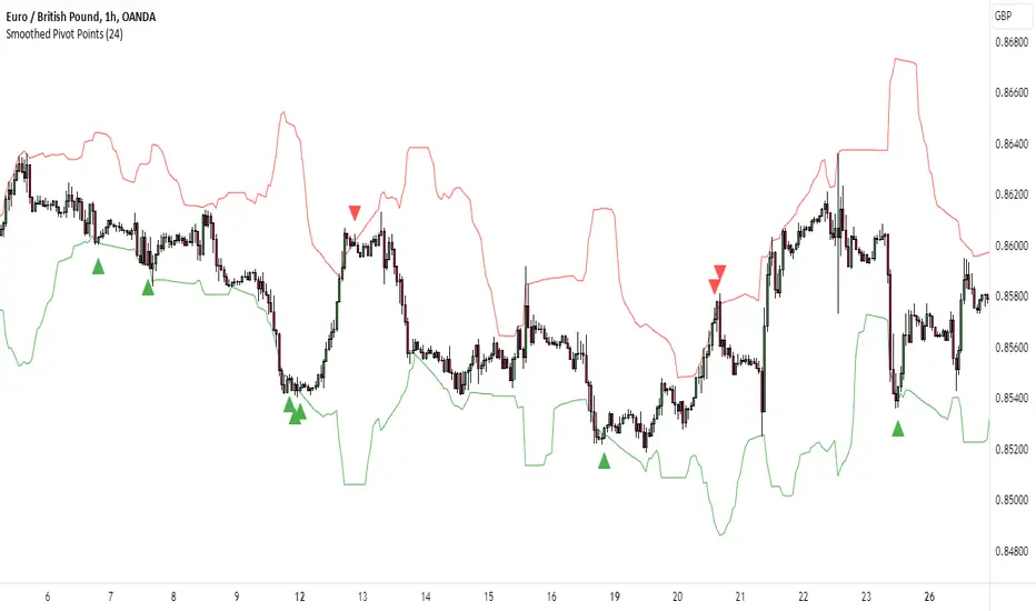
K's Pivot PointsPivot points are a popular technical analysis tool used by traders to identify potential levels of support and resistance in a given timeframe. Pivot points are derived from previous price action and are used to estimate potential price levels where an asset may experience a reversal, breakout, or significant price movement.
The calculation of pivot points involves a simple formula that takes into account the high, low, and close prices from the previous trading session or a specific period. The most commonly used pivot point calculation method is the "Standard" or "Classic" method. Here's the formula:
Pivot Point (P) = (High + Low + Close) / 3
In addition to the pivot point itself, several support and resistance levels are calculated based on the pivot point value.
K's Pivot Points try to enhance them by incorporating multiple elements and by applying a re-integration strategy to validate two events:
* Found_Support: This event represents a basing market that is bound to recover or at least shape a bounce.
* Found_Resistance: This event represents a toppish market that is bound to consolidate or at least shape a pause.
K's Pivot Points are calculated following these steps:
1. Calculate the highest of highs for the previous 24 periods (preferably hours).
2. Calculate the lowest of lows for the previous 24 periods (preferably hours).
3. Calculate a 24-period (preferably hours) moving average of the close price.
4. Calculate K's Pivot Point as the average between the three previous step.
5. To find the support, use this formula: Support = (Lowest K's pivot point of the last 12 periods * 2) - Step 1
6. To find the resistance, use this formula: Resistance = (Highest K's pivot point of the last 12 periods * 2) - Step 2
The re-integration strategy to find support and resistance areas is as follows:
* A support has been found if the market breaks the support and shapes a close above it afterwards.
* A resistance has been found if the market surpasses the resistance and shapes a close below it afterwards.
The lookback period (whether 24 and 12) can be modified but the default versions work well.
WaveTrend 4h/24mWaveTrend 4h/24m is a trading tool based on two WaveTrend timeframes.
For this script the WaveTrend calculations made by LazyBear were used. WaveTrend is a widely used indicator for finding direction of an asset.
The strategy is developed by Youtuber Jayson Casper. The main strategy on the 4 hour and 24 minute timeframes, this will be the default timeframes. Timeframes can be adjusted in the indicator interface.
With Jaysons' we wait for both timeframes to have last printed a green dot for longs, and both timeframes to have last printed a red dot for shorts. When this occurs a green diamond will be printed for longs, a red diamond for shorts.
Make sure to always use the chart from the smallest timeframe you're using, so by defaults use the 24 minute chart.
Features of the indicator:
- WaveTrend Timeframe 1 (Blue/Lightblue wave).
- WaveTrend Timeframe 2 (Blue/Purple line with filled background between the lines).
- VWAP (Yellow wave which is turned off by default)
- Green/Red Diamonds
What to look for?
This script is all about the Green and Red Diamonds.
A Green diamond will be printed when on both the 4 hour and 24 minute timeframe the last printed dot was a green dot.
A Red diamond will be printed when on both the 4 hour and 24 minute timeframe the last printed dot was a red dot.
What are the Green and Red Diamonds based on?
When both VWAP timeframes are ABOVE 0, a green diamond will be printed. This is equivalent to the last dot on both WaveTrend timeframes being a green dot.
When both VWAP timeframes are BELOW 0, a red diamond will be printed. This is equivalent to the last dot on both WaveTrend timeframes being a red dot.
Happy Trading!

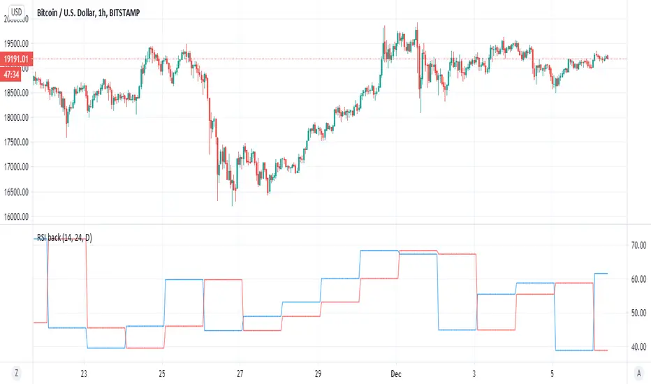
RSI backsimple indicator that based on difference between current RSI and past RSI (historic)
so lets say if take 1 hour chart then in a day there are 24 hour
so our RSI back if we put close will be the rsi of 24 hour before and this we compare it to the current rsi
if the current is above the past one then the signal is bullish , and vice versa. (similar logic to system of buy that based on close yesterday compare open of today)
so to this logic we can add no security MTF to make it nicer
blue line is current MTF RSI , red line is historic RSI based on the number of candles we choose
when blue over red is bullish ,red over blue is bearish
same on 4 hour mTF '1 hour chart and 24 candle back
RSI Correlation with future priceThis script measures the correlation of the hourly RSI of 24 hours ago with the difference of price between now and the price 24 hours ago. In other words, this is an indicator which measures the predictive power of the RSI.
Green means that the price is strongly correlated with the past RSI (which is the normal state when the market is flat and there is no news).
Red means that the price is inversely correlated with the past RSI.
The hourly RSI is a leading indicator which enables you to (sort of) see into the future. It shows you how the current price is, compared to the price 24 (or 48) hours into the future.
If the RSI is low, it means the current price is low compared to the future price, and if the RSI is high, it means the current price is high compared to the future price.
So the hourly RSI really correlates (in the way I described) to the price 24 hours in the future.
Except when it doesn't!!!
What happens when the correlation breaks (RED on this indicator)? Usually there are important news - a strong signal external to the chart. There are either economy at large news, or security-specific news.
Following a strong break of this RSI-future price correlation, some cash can be made by understanding what happened and playing the restoration of the RSI-price correlation.

RSI_SpeedUp_Volume measures the speed of purchases.If the RSI indicator shows the dominance of purchases over sales, it is interesting to know the speed of purchases. We calculate the speed using the wt indicator. We compute WT (RSI,len). Setting and designation of indicator RSI_SpeedUP. The RSI lines you are looking for are shown in smooth lines. The speed is shown by stepped lines.
In the indicator RSI and speed are calculated in two ways. The first method-calculations are made from the closing price.
The second way is from the volume price. Volume price is the closing price multiplied by volume. Basic settings of the RSI_SpeedUp-V indicator (1,24,9,40,14). What they mean?
RSI is calculated for two periods 24 and 9. The first parameter in the setting is "1", that the display of lines will be from the first period = 24. If the parameter is "2", the lines will be displayed from the second period = 9.
If the parameter is "3", the display will be simultaneously from both periods.
The fourth parameter " 40 " shows the width of the green and pink areas.
The fifth parameter " 14 " is the period with which the wt rate is calculated(rsi,14).
By default, the indicator window displays only the rates from the simple price and the volume price. In order to enable the display of RSI lines, press the "vkl RSI"button.
The blue line is RSI (close). Blue line-RSI (close*volume). Stepped green-speed from simple price wt(rsi (close)). Step brown line-speed from the volume price wt(rsi (close*volume)).
How to use. The volume price starts to react to the trend change earlier. Long before the reversal, it changes its direction. Comparison with the simple price speed line gives additional information about the market mood.
Good luck with your trading.
--------------------------
Если индикатор RSI показывает доминирование покупок над продажами, то интересно знать скорость покупок. Скорость мы вычисляем с помощью индикатора WT. Мы вычисляем WT ( RSI,len). Настройки и обозначения индикатора RSI_SpeedUP. Искомые линии RSI показаны гладкими линиями. Скорость показана ступенчатыми линиями.
В индикаторе RSI и скорость вычисляются двумя способами. Первый способ - вычисления производятся от цены закрытия. Второй способ от объемной цены. Объемная цена это цена закрытия умноженная на объем. Базовые настройки индикатора RSI_SpeedUp-V (1,24,9,40,14). Что они означают?
RSI вычисляется для двух периодов 24 и 9. Первый параметр в настройке "1" , что отображение линий будет от первого периода = 24. Если параметр "2", то отображение линий будет от второго периода = 9. Если параметр "3", то отображение будет одновременно от обоих периодов.
Четвертый параметр "40" показывает ширину области зеленой и розовой.
Пятый параметр "14" это период с которым вычисляется скорость wt(rsi,14).
По умолчанию в окне индикатора отображаются только скорости от простой цены и от объемной цены. Для того чтобы включить отображение линий RSI надо нажать кнопочку "vkl RSI".
Синяя линия - RSI (close). Голубая линия - RSI (close*volume). Ступенчатая зеленая - скорость от простой цены wt(rsi(close)). Ступенчатая коричневая линия - скорость от объемной цены wt(rsi(close*volume)).
Как пользоваться. Объемная цена раньше начинает реагировать на изменение тенденции. Задолго до разворота она изменяет своё направление. Сравнение с линией скорости простой цены дает дополнительную информацию о настроении рынка.
Успехов Вам в торговле.

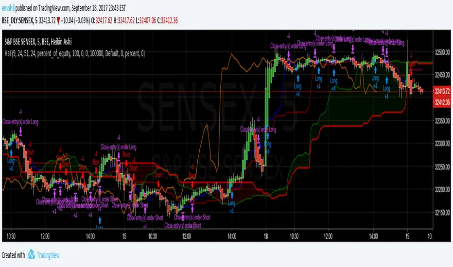
Heiken Ashi + Ichimoku Kinko Hyo StrategyHeikin-Ashi:
Instead of using the open-high-low-close (OHLC) bars like standard candlestick charts, it uses a modified formula. Out of which only following two are used in this strategy.
High = Max (High,Open,Close)
Low = Min (Low,Open, Close)
Ichimoku Kinko Hyo:
The Ichimoku Kinko Hyo system includes five kinds of signal, of which this strategy uses four signals i.e. Tenkan Sen / Kijun Sen Cross, price crosses the Kijun Sen, Chikou Span and Kumo. Although the Chikou Span, Senkou Span A and Senkou Span B (Kumo) are shifted into the past/future, these trigger signals enhances the strategy.
The Tenkan Sen, also known as the Turning or Conversion line, is a moving average of the highest high and lowest low over the last 9 periods in this strategy.
The Kijun Sen, also known as the Standard or Base line, is a moving average of the highest high and lowest low over the last 24 periods in this strategy.
The Chikou Span, also known as the Lagging line, is the closing price plotted 24 periods behind in this strategy.
The Senkou Span A, also known as the 1st leading line, is a moving average of the Tenkan Sen and Kijun Sen and is plotted 24 periods ahead in this strategy.
The Senkou Span B, also known as the 2nd leading line, is a moving average of the highest high and lowest low over the last 51 trading days is plotted 24 periods ahead in this strategy.
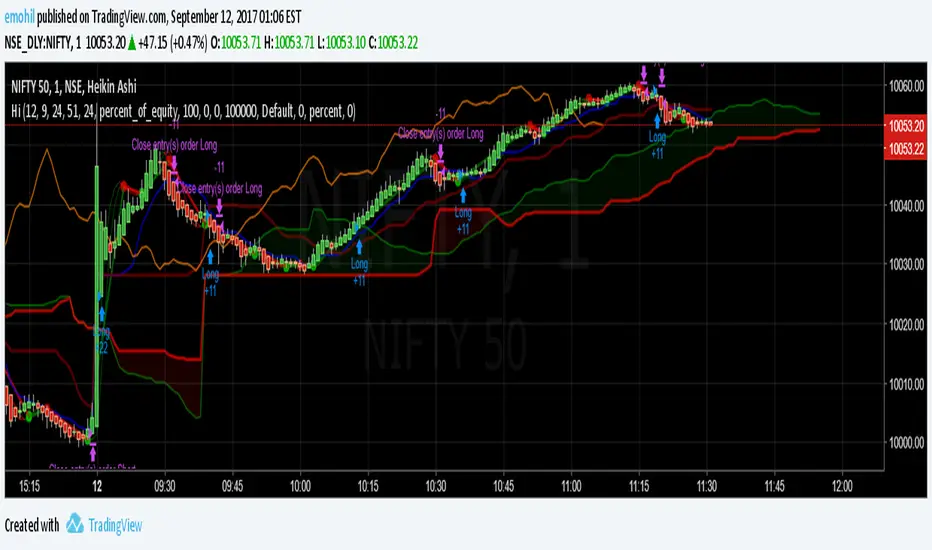
Hull MA-X + Ichimoku Kinko Hyo StrategyHull MA-X:
The Hull MA involves the weighted moving average ( WMA ) in its calculation.
First, calculate the WMA with period (n / 2) and multiply this by 2. Remember ‘n’ is the time period configurable based on the trader’s requirement.
Second, calculate the WMA for period “n” and subtract if from the first step. Thirdly, calculate the weighted moving average with period sqrt (n) using the data from the second step. You can take a look at the below formula:
Hull MA= WMA (2*WMA (n/2) − WMA (n)), sqrt (n))
The default setting is 12 periods in this strategy, fast Hull MA crossing slow Hull MA will generate a circle on charts.
Ichimoku Kinko Hyo:
The Ichimoku Kinko Hyo system includes five kinds of signal, of which this strategy uses four signals i.e. Tenkan Sen / Kijun Sen Cross, price crosses the Kijun Sen, Chikou Span and Kumo. Although the Chikou Span, Senkou Span A and Senkou Span B (Kumo) are shifted into the past/future, these trigger signals enhances the strategy.
The Tenkan Sen, also known as the Turning or Conversion line, is a moving average of the highest high and lowest low over the last 9 periods in this strategy.
The Kijun Sen, also known as the Standard or Base line, is a moving average of the highest high and lowest low over the last 24 periods in this strategy.
The Chikou Span, also known as the Lagging line, is the closing price plotted 24 periods behind in this strategy.
The Senkou Span A, also known as the 1st leading line, is a moving average of the Tenkan Sen and Kijun Sen and is plotted 24 periods ahead in this strategy.
The Senkou Span B, also known as the 2nd leading line, is a moving average of the highest high and lowest low over the last 51 trading days is plotted 24 periods ahead in this strategy.
As with most technical analysis methods, Ichimoku is likely to produce frequent conflicting signals in non-trending markets, So in addition to Ichimoku Kinko Hyo, the Hull MA is used, which is popular amongst some day traders, in combination it attempts to give an accurate signal by eliminating lags and improving the smoothness of the line.
The Hull MA Cross in combination with Ichimoku Kinko Hyo signals tries to give an accurate signal by eliminating lags and improve the smoothness of price activity. Please note that price trends can and do change often, so your readings of the charts and this trading system should be probabilistic, rather than predictive.
Six Meridian Divine Swords [theUltimator5]The Six Meridian Divine Sword is a legendary martial arts technique in the classic wuxia novel “Demi-Gods and Semi-Devils” (天龙八部) by Jin Yong (金庸). The technique uses powerful internal energy (qi) to shoot invisible sword-like energy beams from the six meridians of the hand. Each of the six fingers/meridians corresponds to a “sword,” giving six different sword energies.
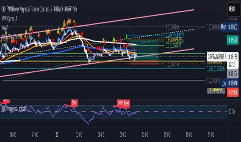
The Six Meridian Divine Swords indicator is a compact “signal dashboard” that fuses six classic indicators (fingers)—MACD, KDJ, RSI, LWR (Williams %R), BBI, and MTM—into one pane. Each row is a traffic-light dot (green/bullish, red/bearish, gray/neutral). When all six align, the script draws a confirmation line (“All Bullish” or “All Bearish”). It’s designed for quick consensus reads across trend, momentum, and overbought/oversold conditions.
How to Read the Dashboard
The pane has 6 horizontal rows (explained in depth later):
MACD
KDJ
RSI
LWR (Larry Williams %R)
BBI (Bull & Bear Index)
MTM (Momentum)
Each tick in the row is a dot, with sentiment identified by a color.
Green = bullish condition met
Red = bearish condition met
Gray = inside a neutral band (filtering chop), shown when Use Neutral (Gray) Colors is ON
There are two lines that track the dots on the top or bottom of the pane.
All Bullish Signal Line: appears only if all 6 are strongly bullish (default color = white)
All Bearish Signal Line: appears only if all 6 are strongly bearish (default color = fuchsia)
The Six Meridians (Indicators) — What They Mean:
1) MACD — Trend & Momentum
What it is: A trend-following momentum indicator based on the relationship between two moving averages (typically 12-EMA and 26-EMA)
Logic used: Classic MACD line (EMA12−EMA26) vs its 9-EMA signal.
Bullish: MACD > Signal and |MACD−Signal| > Neutral Threshold
Bearish: MACD < Signal and |diff| > threshold
Neutral: |diff| ≤ threshold
Why: Small crosses can whipsaw. The neutral band ignores tiny separations to reduce noise.
Inputs: Fast/Slow/Signal lengths, Neutral Threshold.
2) KDJ — Stochastic with J-line boost
What it is: A variation of the stochastic oscillator popular in Chinese trading systems
Logic used: K = SMA(Stochastic, smooth), D = SMA(K, smooth), J = 3K − 2D.
Bullish: K > D and |K−D| > 2
Bearish: K < D and |K−D| > 2
Neutral: |K−D| ≤ 2
Why: K–D separation filters tiny wiggles; J offers an “extreme” early-warning context in the value label.
Inputs: Length, Smoothing.
3) RSI — Momentum balance (0–100)
What it is: A momentum oscillator measuring speed and magnitude of price changes (0–100)
Logic used: RSI(N).
Bullish: RSI > 50 + Neutral Zone
Bearish: RSI < 50 − Neutral Zone
Neutral: Between those bands
Why: Centerline/adaptive bands (around 50) give a directional bias without relying on fixed 70/30.
Inputs: Length, Neutral Zone (± around 50).
4) LWR (Williams %R) — Overbought/Oversold
What it is: An oscillator similar to stochastic, measuring how close the close is to the high-low range over N periods
Logic used: %R over N bars (0 to −100).
Bullish: %R > −50 + Neutral Zone
Bearish: %R < −50 − Neutral Zone
Neutral: Between those bands
Why: Uses a centered band around −50 instead of only −20/−80, making it act like a directional filter.
Inputs: Length, Neutral Zone (± around −50).
5) BBI (Bull & Bear Index) — Smoothed trend bias
What it is: A composite moving average, essentially the average of several different moving averages (often 3, 6, 12, 24 periods)
Logic used: Average of 4 SMAs (3/6/12/24 by default):
BBI = (MA3 + MA6 + MA12 + MA24) / 4
Bullish: Close > BBI and |Close−BBI| > 0.2% of BBI
Bearish: Close < BBI and |diff| > threshold
Neutral: |diff| ≤ threshold
Why: Multiple MAs blended together reduce single-MA whipsaw. A dynamic 0.2% band ignores tiny drift.
Inputs: 4 lengths (default 3/6/12/24). Threshold is auto-scaled at 0.2% of BBI.
6) MTM (Momentum) — Rate of change in price
What it is: A simple measure of rate of change
Logic used: MTM = Close − Close
Bullish: MTM > 0.5% of Close
Bearish: MTM < −0.5% of Close
Neutral: |MTM| ≤ threshold
Why: A percent-based gate adapts across prices (e.g., $5 vs $500) and mutes insignificant moves.
Inputs: Length. Threshold auto-scaled to 0.5% of current Close.
Display & Inputs You Can Tweak
🎨 Use Neutral (Gray) Colors
ON (default): 3-color mode with clear “no-trade”/“weak” states.
OFF: classic binary (green/red) without neutral filtering.

80% Rule Indicator (ETH Session + SVP Prior Session)I created this script to show the 80% opportunity on chart if setting lines up.
"80% rule: Open outside the vah or Val. Spend 30 mins outside there then break back inside spend 15 mins below or above depending which way u broke. Then come back and retest the vah/val and take it to the poc as a first target with the final target being the other Val/vah "
📌 Script Summary
The "80% Rule Indicator (ETH Session + SVP Prior Session)" overlays your chart with prior session value area levels (VAH, VAL, and POC) calculated from extended-hours 30-minute data. It tracks when the price reenters the value area and confirms 80% Rule setups during your chosen trading session. You can optionally trigger alerts, show/hide market sessions, and fine-tune line appearance for a clean, modular workflow.
⚙️ Options & Settings Breakdown
- Use 24-Hour Session (All Markets)
When checked, the indicator ignores time zones and tracks signals during a full 24-hour period (0000-0000), helpful if you're outside U.S. trading hours or want consistent behavior globally.
- Market Session
Dropdown to select one of three key market zones:
- New York (09:30–16:00 ET)
- London (08:00–16:30 local)
- Tokyo (09:00–15:00 local)
Used to gate entry signals during relevant hours unless you choose the 24-hour option.
- Show PD VAH/VAL/POC Lines
Toggle to show or hide prior day’s levels (based on the 30-min extended session). Turning this off removes both the lines and their white text labels.
- Extend Lines Right
When enabled, the VAH/VAL/POC lines extend into the current day’s session. If disabled, they appear only at their anchor point.
- Highlight Selected Session
Adds a soft blue background to help visualize the active session you selected.
- Enable Alert Conditions
Allows TradingView alerts to be created for long/short 80% Rule entries.
- Enable Audible Alerts
Plays an in-chart sound with a popup message (“80% Rule LONG” or “SHORT”) when signals trigger. Requires the chart to be active and sounds enabled in TradingView.

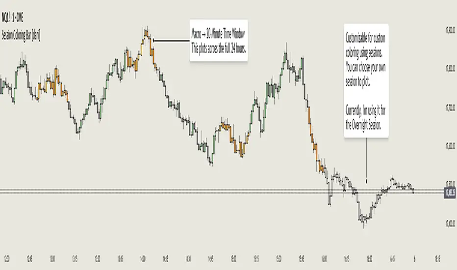
Session Coloring Bar with ICT Macro [dani]The Session Coloring Bar is customizable Pine Script indicator designed to visually enhance your charts by applying unique colors to specific trading sessions or timeframes. This tool allows traders to easily identify and differentiate between macro sessions (e.g., 24-hour cycles) and custom-defined sessions (e.g., Session A, Session B), making it ideal for analyzing market activity during specific periods.
In the context of trading, the term "ICT Macro" , as discussed by Michael J. Huddleston (ICT), refers to specific timeframes or "windows" where market behavior often follows predictable patterns. Traders typically focus on the last 10 minutes of an hour and the first 10 minutes of the next hour (e.g., 0150-0210 , 0050-0110 , or 0950-1010 ) to identify key price movements, liquidity shifts, or market inefficiencies.
This script highlights these macro timeframes, enabling traders to visually analyze price action during these critical periods. Use this tool to support your strategy, but always combine it with your own analysis and risk management.
With this indicator, you can:
Highlight Macro Sessions : Automatically color bars based on predefined 24-hour macro sessions.
Customize Session Settings : Define up to three custom sessions (A & B) with individual start/end times, visibility toggles, and unique bar colors.
Timeframe Filtering : Hide session coloring above a specified timeframe to avoid clutter on higher timeframes.
Personal Notes : Add comments to each session for better organization and quick reference.
Dynamic Color Logic : Bars are colored based on their direction (up, down, or neutral) within the active session.
How to Use:
Enable/Disable Sessions :
Use the Show Coloring toggle to enable or disable session coloring for Macro, Session A, Session B, or Session C.
Set Session Times :
Define the start and end times for each session in the format HHMM-HHMM (e.g., 1600-0930 for an overnight session).
Choose Colors :
Assign unique colors for upward (Bar Up) and downward (Bar Down) bars within each session.
Adjust Timeframe Visibility :
Use the Hide above this TF input to specify the maximum timeframe where session coloring will be visible.
Add Notes :
Use the Comment field to add personal notes or labels for each session.
Example Use Cases:
Overnight Sessions :
Highlight overnight trading hours (e.g., 1600-0930) to analyze price action during low liquidity periods.
Asian/European/US Sessions : Define separate sessions for major trading regions to track regional market behavior.
Macro Analysis : Use the predefined 24-hour macro sessions to study hourly price movements across a full trading day.
Disclaimer:
The Session Coloring Bar is not a trading signal generator and does not predict market direction or provide buy/sell signals. Instead, it is a visualization tool designed to help you identify and analyze specific trading sessions or timeframes on your chart. By highlighting key sessions and their corresponding price movements, this indicator enables you to focus on periods of interest and make more informed trading decisions.
Thank you for choosing this indicator! I hope it becomes a valuable part of your trading toolkit. Remember, trading is a journey, and having the right tools can make all the difference. Whether you're a seasoned trader or just starting out, this indicator is designed to help you stay organized and focused on what matters most—price action. Happy trading, and may your charts be ever in your favor! 😊
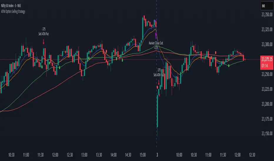
ATM Option Selling StrategyATM Option Selling Strategy – Explained
This strategy is designed for intraday option selling based on the 9/15 EMA crossover, 50/80 MA trend filter, and RSI 50 level. It ensures that all trades are exited before market close (3:24 PM IST).
. Indicators Used:
9 EMA & 15 EMA → For short-term trend identification.
50 MA & 80 MA → To determine the overall trend.
RSI (14) → To confirm momentum (above or below 50 level).
2. Entry Conditions:
🔴 Sell ATM Call (CE) when:
Price is below 50 & 80 MA (Bearish trend).
9 EMA crosses below 15 EMA (Short-term trend turns bearish).
RSI is below 50 (Momentum confirms weakness).
🟢 Sell ATM Put (PE) when:
Price is above 50 & 80 MA (Bullish trend).
9 EMA crosses above 15 EMA (Short-term trend turns bullish).
RSI is above 50 (Momentum confirms strength).
3. Position Sizing & Risk Management:
Sell 375 quantity per trade (Lot size).
50-Point Stop Loss → If option premium moves against us by 50 points, exit.
50-Point Take Profit → If option premium moves in our favor by 50 points, book profit.
Exit all trades at 3:24 PM IST → No overnight positions.
4. Exit Conditions:
✅ Stop Loss or Take Profit Hits → Automatically exits based on a 50-point move.
✅ Time-Based Exit at 3:24 PM → Ensures no open positions at market close.
Why This Works?
✔ Trend Confirmation → 50/80 MA ensures we only sell options in the direction of the market trend.
✔ Momentum Confirmation → RSI prevents entering weak trades.
✔ Controlled Risk → SL and TP protect against large losses.
✔ No Overnight Risk → All trades close before market close.
Universal Ratio Trend Matrix [InvestorUnknown]The Universal Ratio Trend Matrix is designed for trend analysis on asset/asset ratios, supporting up to 40 different assets. Its primary purpose is to help identify which assets are outperforming others within a selection, providing a broad overview of market trends through a matrix of ratios. The indicator automatically expands the matrix based on the number of assets chosen, simplifying the process of comparing multiple assets in terms of performance.
Key features include the ability to choose from a narrow selection of indicators to perform the ratio trend analysis, allowing users to apply well-defined metrics to their comparison.
Drawback: Due to the computational intensity involved in calculating ratios across many assets, the indicator has a limitation related to loading speed. TradingView has time limits for calculations, and for users on the basic (free) plan, this could result in frequent errors due to exceeded time limits. To use the indicator effectively, users with any paid plans should run it on timeframes higher than 8h (the lowest timeframe on which it managed to load with 40 assets), as lower timeframes may not reliably load.
Indicators:
RSI_raw: Simple function to calculate the Relative Strength Index (RSI) of a source (asset price).
RSI_sma: Calculates RSI followed by a Simple Moving Average (SMA).
RSI_ema: Calculates RSI followed by an Exponential Moving Average (EMA).
CCI: Calculates the Commodity Channel Index (CCI).
Fisher: Implements the Fisher Transform to normalize prices.
Utility Functions:
f_remove_exchange_name: Strips the exchange name from asset tickers (e.g., "INDEX:BTCUSD" to "BTCUSD").
f_remove_exchange_name(simple string name) =>
string parts = str.split(name, ":")
string result = array.size(parts) > 1 ? array.get(parts, 1) : name
result
f_get_price: Retrieves the closing price of a given asset ticker using request.security().
f_constant_src: Checks if the source data is constant by comparing multiple consecutive values.
Inputs:
General settings allow users to select the number of tickers for analysis (used_assets) and choose the trend indicator (RSI, CCI, Fisher, etc.).
Table settings customize how trend scores are displayed in terms of text size, header visibility, highlighting options, and top-performing asset identification.
The script includes inputs for up to 40 assets, allowing the user to select various cryptocurrencies (e.g., BTCUSD, ETHUSD, SOLUSD) or other assets for trend analysis.
Price Arrays:
Price values for each asset are stored in variables (price_a1 to price_a40) initialized as na. These prices are updated only for the number of assets specified by the user (used_assets).
Trend scores for each asset are stored in separate arrays
// declare price variables as "na"
var float price_a1 = na, var float price_a2 = na, var float price_a3 = na, var float price_a4 = na, var float price_a5 = na
var float price_a6 = na, var float price_a7 = na, var float price_a8 = na, var float price_a9 = na, var float price_a10 = na
var float price_a11 = na, var float price_a12 = na, var float price_a13 = na, var float price_a14 = na, var float price_a15 = na
var float price_a16 = na, var float price_a17 = na, var float price_a18 = na, var float price_a19 = na, var float price_a20 = na
var float price_a21 = na, var float price_a22 = na, var float price_a23 = na, var float price_a24 = na, var float price_a25 = na
var float price_a26 = na, var float price_a27 = na, var float price_a28 = na, var float price_a29 = na, var float price_a30 = na
var float price_a31 = na, var float price_a32 = na, var float price_a33 = na, var float price_a34 = na, var float price_a35 = na
var float price_a36 = na, var float price_a37 = na, var float price_a38 = na, var float price_a39 = na, var float price_a40 = na
// create "empty" arrays to store trend scores
var a1_array = array.new_int(40, 0), var a2_array = array.new_int(40, 0), var a3_array = array.new_int(40, 0), var a4_array = array.new_int(40, 0)
var a5_array = array.new_int(40, 0), var a6_array = array.new_int(40, 0), var a7_array = array.new_int(40, 0), var a8_array = array.new_int(40, 0)
var a9_array = array.new_int(40, 0), var a10_array = array.new_int(40, 0), var a11_array = array.new_int(40, 0), var a12_array = array.new_int(40, 0)
var a13_array = array.new_int(40, 0), var a14_array = array.new_int(40, 0), var a15_array = array.new_int(40, 0), var a16_array = array.new_int(40, 0)
var a17_array = array.new_int(40, 0), var a18_array = array.new_int(40, 0), var a19_array = array.new_int(40, 0), var a20_array = array.new_int(40, 0)
var a21_array = array.new_int(40, 0), var a22_array = array.new_int(40, 0), var a23_array = array.new_int(40, 0), var a24_array = array.new_int(40, 0)
var a25_array = array.new_int(40, 0), var a26_array = array.new_int(40, 0), var a27_array = array.new_int(40, 0), var a28_array = array.new_int(40, 0)
var a29_array = array.new_int(40, 0), var a30_array = array.new_int(40, 0), var a31_array = array.new_int(40, 0), var a32_array = array.new_int(40, 0)
var a33_array = array.new_int(40, 0), var a34_array = array.new_int(40, 0), var a35_array = array.new_int(40, 0), var a36_array = array.new_int(40, 0)
var a37_array = array.new_int(40, 0), var a38_array = array.new_int(40, 0), var a39_array = array.new_int(40, 0), var a40_array = array.new_int(40, 0)
f_get_price(simple string ticker) =>
request.security(ticker, "", close)
// Prices for each USED asset
f_get_asset_price(asset_number, ticker) =>
if (used_assets >= asset_number)
f_get_price(ticker)
else
na
// overwrite empty variables with the prices if "used_assets" is greater or equal to the asset number
if barstate.isconfirmed // use barstate.isconfirmed to avoid "na prices" and calculation errors that result in empty cells in the table
price_a1 := f_get_asset_price(1, asset1), price_a2 := f_get_asset_price(2, asset2), price_a3 := f_get_asset_price(3, asset3), price_a4 := f_get_asset_price(4, asset4)
price_a5 := f_get_asset_price(5, asset5), price_a6 := f_get_asset_price(6, asset6), price_a7 := f_get_asset_price(7, asset7), price_a8 := f_get_asset_price(8, asset8)
price_a9 := f_get_asset_price(9, asset9), price_a10 := f_get_asset_price(10, asset10), price_a11 := f_get_asset_price(11, asset11), price_a12 := f_get_asset_price(12, asset12)
price_a13 := f_get_asset_price(13, asset13), price_a14 := f_get_asset_price(14, asset14), price_a15 := f_get_asset_price(15, asset15), price_a16 := f_get_asset_price(16, asset16)
price_a17 := f_get_asset_price(17, asset17), price_a18 := f_get_asset_price(18, asset18), price_a19 := f_get_asset_price(19, asset19), price_a20 := f_get_asset_price(20, asset20)
price_a21 := f_get_asset_price(21, asset21), price_a22 := f_get_asset_price(22, asset22), price_a23 := f_get_asset_price(23, asset23), price_a24 := f_get_asset_price(24, asset24)
price_a25 := f_get_asset_price(25, asset25), price_a26 := f_get_asset_price(26, asset26), price_a27 := f_get_asset_price(27, asset27), price_a28 := f_get_asset_price(28, asset28)
price_a29 := f_get_asset_price(29, asset29), price_a30 := f_get_asset_price(30, asset30), price_a31 := f_get_asset_price(31, asset31), price_a32 := f_get_asset_price(32, asset32)
price_a33 := f_get_asset_price(33, asset33), price_a34 := f_get_asset_price(34, asset34), price_a35 := f_get_asset_price(35, asset35), price_a36 := f_get_asset_price(36, asset36)
price_a37 := f_get_asset_price(37, asset37), price_a38 := f_get_asset_price(38, asset38), price_a39 := f_get_asset_price(39, asset39), price_a40 := f_get_asset_price(40, asset40)
Universal Indicator Calculation (f_calc_score):
This function allows switching between different trend indicators (RSI, CCI, Fisher) for flexibility.
It uses a switch-case structure to calculate the indicator score, where a positive trend is denoted by 1 and a negative trend by 0. Each indicator has its own logic to determine whether the asset is trending up or down.
// use switch to allow "universality" in indicator selection
f_calc_score(source, trend_indicator, int_1, int_2) =>
int score = na
if (not f_constant_src(source)) and source > 0.0 // Skip if you are using the same assets for ratio (for example BTC/BTC)
x = switch trend_indicator
"RSI (Raw)" => RSI_raw(source, int_1)
"RSI (SMA)" => RSI_sma(source, int_1, int_2)
"RSI (EMA)" => RSI_ema(source, int_1, int_2)
"CCI" => CCI(source, int_1)
"Fisher" => Fisher(source, int_1)
y = switch trend_indicator
"RSI (Raw)" => x > 50 ? 1 : 0
"RSI (SMA)" => x > 50 ? 1 : 0
"RSI (EMA)" => x > 50 ? 1 : 0
"CCI" => x > 0 ? 1 : 0
"Fisher" => x > x ? 1 : 0
score := y
else
score := 0
score
Array Setting Function (f_array_set):
This function populates an array with scores calculated for each asset based on a base price (p_base) divided by the prices of the individual assets.
It processes multiple assets (up to 40), calling the f_calc_score function for each.
// function to set values into the arrays
f_array_set(a_array, p_base) =>
array.set(a_array, 0, f_calc_score(p_base / price_a1, trend_indicator, int_1, int_2))
array.set(a_array, 1, f_calc_score(p_base / price_a2, trend_indicator, int_1, int_2))
array.set(a_array, 2, f_calc_score(p_base / price_a3, trend_indicator, int_1, int_2))
array.set(a_array, 3, f_calc_score(p_base / price_a4, trend_indicator, int_1, int_2))
array.set(a_array, 4, f_calc_score(p_base / price_a5, trend_indicator, int_1, int_2))
array.set(a_array, 5, f_calc_score(p_base / price_a6, trend_indicator, int_1, int_2))
array.set(a_array, 6, f_calc_score(p_base / price_a7, trend_indicator, int_1, int_2))
array.set(a_array, 7, f_calc_score(p_base / price_a8, trend_indicator, int_1, int_2))
array.set(a_array, 8, f_calc_score(p_base / price_a9, trend_indicator, int_1, int_2))
array.set(a_array, 9, f_calc_score(p_base / price_a10, trend_indicator, int_1, int_2))
array.set(a_array, 10, f_calc_score(p_base / price_a11, trend_indicator, int_1, int_2))
array.set(a_array, 11, f_calc_score(p_base / price_a12, trend_indicator, int_1, int_2))
array.set(a_array, 12, f_calc_score(p_base / price_a13, trend_indicator, int_1, int_2))
array.set(a_array, 13, f_calc_score(p_base / price_a14, trend_indicator, int_1, int_2))
array.set(a_array, 14, f_calc_score(p_base / price_a15, trend_indicator, int_1, int_2))
array.set(a_array, 15, f_calc_score(p_base / price_a16, trend_indicator, int_1, int_2))
array.set(a_array, 16, f_calc_score(p_base / price_a17, trend_indicator, int_1, int_2))
array.set(a_array, 17, f_calc_score(p_base / price_a18, trend_indicator, int_1, int_2))
array.set(a_array, 18, f_calc_score(p_base / price_a19, trend_indicator, int_1, int_2))
array.set(a_array, 19, f_calc_score(p_base / price_a20, trend_indicator, int_1, int_2))
array.set(a_array, 20, f_calc_score(p_base / price_a21, trend_indicator, int_1, int_2))
array.set(a_array, 21, f_calc_score(p_base / price_a22, trend_indicator, int_1, int_2))
array.set(a_array, 22, f_calc_score(p_base / price_a23, trend_indicator, int_1, int_2))
array.set(a_array, 23, f_calc_score(p_base / price_a24, trend_indicator, int_1, int_2))
array.set(a_array, 24, f_calc_score(p_base / price_a25, trend_indicator, int_1, int_2))
array.set(a_array, 25, f_calc_score(p_base / price_a26, trend_indicator, int_1, int_2))
array.set(a_array, 26, f_calc_score(p_base / price_a27, trend_indicator, int_1, int_2))
array.set(a_array, 27, f_calc_score(p_base / price_a28, trend_indicator, int_1, int_2))
array.set(a_array, 28, f_calc_score(p_base / price_a29, trend_indicator, int_1, int_2))
array.set(a_array, 29, f_calc_score(p_base / price_a30, trend_indicator, int_1, int_2))
array.set(a_array, 30, f_calc_score(p_base / price_a31, trend_indicator, int_1, int_2))
array.set(a_array, 31, f_calc_score(p_base / price_a32, trend_indicator, int_1, int_2))
array.set(a_array, 32, f_calc_score(p_base / price_a33, trend_indicator, int_1, int_2))
array.set(a_array, 33, f_calc_score(p_base / price_a34, trend_indicator, int_1, int_2))
array.set(a_array, 34, f_calc_score(p_base / price_a35, trend_indicator, int_1, int_2))
array.set(a_array, 35, f_calc_score(p_base / price_a36, trend_indicator, int_1, int_2))
array.set(a_array, 36, f_calc_score(p_base / price_a37, trend_indicator, int_1, int_2))
array.set(a_array, 37, f_calc_score(p_base / price_a38, trend_indicator, int_1, int_2))
array.set(a_array, 38, f_calc_score(p_base / price_a39, trend_indicator, int_1, int_2))
array.set(a_array, 39, f_calc_score(p_base / price_a40, trend_indicator, int_1, int_2))
a_array
Conditional Array Setting (f_arrayset):
This function checks if the number of used assets is greater than or equal to a specified number before populating the arrays.
// only set values into arrays for USED assets
f_arrayset(asset_number, a_array, p_base) =>
if (used_assets >= asset_number)
f_array_set(a_array, p_base)
else
na
Main Logic
The main logic initializes arrays to store scores for each asset. Each array corresponds to one asset's performance score.
Setting Trend Values: The code calls f_arrayset for each asset, populating the respective arrays with calculated scores based on the asset prices.
Combining Arrays: A combined_array is created to hold all the scores from individual asset arrays. This array facilitates further analysis, allowing for an overview of the performance scores of all assets at once.
// create a combined array (work-around since pinescript doesn't support having array of arrays)
var combined_array = array.new_int(40 * 40, 0)
if barstate.islast
for i = 0 to 39
array.set(combined_array, i, array.get(a1_array, i))
array.set(combined_array, i + (40 * 1), array.get(a2_array, i))
array.set(combined_array, i + (40 * 2), array.get(a3_array, i))
array.set(combined_array, i + (40 * 3), array.get(a4_array, i))
array.set(combined_array, i + (40 * 4), array.get(a5_array, i))
array.set(combined_array, i + (40 * 5), array.get(a6_array, i))
array.set(combined_array, i + (40 * 6), array.get(a7_array, i))
array.set(combined_array, i + (40 * 7), array.get(a8_array, i))
array.set(combined_array, i + (40 * 8), array.get(a9_array, i))
array.set(combined_array, i + (40 * 9), array.get(a10_array, i))
array.set(combined_array, i + (40 * 10), array.get(a11_array, i))
array.set(combined_array, i + (40 * 11), array.get(a12_array, i))
array.set(combined_array, i + (40 * 12), array.get(a13_array, i))
array.set(combined_array, i + (40 * 13), array.get(a14_array, i))
array.set(combined_array, i + (40 * 14), array.get(a15_array, i))
array.set(combined_array, i + (40 * 15), array.get(a16_array, i))
array.set(combined_array, i + (40 * 16), array.get(a17_array, i))
array.set(combined_array, i + (40 * 17), array.get(a18_array, i))
array.set(combined_array, i + (40 * 18), array.get(a19_array, i))
array.set(combined_array, i + (40 * 19), array.get(a20_array, i))
array.set(combined_array, i + (40 * 20), array.get(a21_array, i))
array.set(combined_array, i + (40 * 21), array.get(a22_array, i))
array.set(combined_array, i + (40 * 22), array.get(a23_array, i))
array.set(combined_array, i + (40 * 23), array.get(a24_array, i))
array.set(combined_array, i + (40 * 24), array.get(a25_array, i))
array.set(combined_array, i + (40 * 25), array.get(a26_array, i))
array.set(combined_array, i + (40 * 26), array.get(a27_array, i))
array.set(combined_array, i + (40 * 27), array.get(a28_array, i))
array.set(combined_array, i + (40 * 28), array.get(a29_array, i))
array.set(combined_array, i + (40 * 29), array.get(a30_array, i))
array.set(combined_array, i + (40 * 30), array.get(a31_array, i))
array.set(combined_array, i + (40 * 31), array.get(a32_array, i))
array.set(combined_array, i + (40 * 32), array.get(a33_array, i))
array.set(combined_array, i + (40 * 33), array.get(a34_array, i))
array.set(combined_array, i + (40 * 34), array.get(a35_array, i))
array.set(combined_array, i + (40 * 35), array.get(a36_array, i))
array.set(combined_array, i + (40 * 36), array.get(a37_array, i))
array.set(combined_array, i + (40 * 37), array.get(a38_array, i))
array.set(combined_array, i + (40 * 38), array.get(a39_array, i))
array.set(combined_array, i + (40 * 39), array.get(a40_array, i))
Calculating Sums: A separate array_sums is created to store the total score for each asset by summing the values of their respective score arrays. This allows for easy comparison of overall performance.
Ranking Assets: The final part of the code ranks the assets based on their total scores stored in array_sums. It assigns a rank to each asset, where the asset with the highest score receives the highest rank.
// create array for asset RANK based on array.sum
var ranks = array.new_int(used_assets, 0)
// for loop that calculates the rank of each asset
if barstate.islast
for i = 0 to (used_assets - 1)
int rank = 1
for x = 0 to (used_assets - 1)
if i != x
if array.get(array_sums, i) < array.get(array_sums, x)
rank := rank + 1
array.set(ranks, i, rank)
Dynamic Table Creation
Initialization: The table is initialized with a base structure that includes headers for asset names, scores, and ranks. The headers are set to remain constant, ensuring clarity for users as they interpret the displayed data.
Data Population: As scores are calculated for each asset, the corresponding values are dynamically inserted into the table. This is achieved through a loop that iterates over the scores and ranks stored in the combined_array and array_sums, respectively.
Automatic Extending Mechanism
Variable Asset Count: The code checks the number of assets defined by the user. Instead of hardcoding the number of rows in the table, it uses a variable to determine the extent of the data that needs to be displayed. This allows the table to expand or contract based on the number of assets being analyzed.
Dynamic Row Generation: Within the loop that populates the table, the code appends new rows for each asset based on the current asset count. The structure of each row includes the asset name, its score, and its rank, ensuring that the table remains consistent regardless of how many assets are involved.
// Automatically extending table based on the number of used assets
var table table = table.new(position.bottom_center, 50, 50, color.new(color.black, 100), color.white, 3, color.white, 1)
if barstate.islast
if not hide_head
table.cell(table, 0, 0, "Universal Ratio Trend Matrix", text_color = color.white, bgcolor = #010c3b, text_size = fontSize)
table.merge_cells(table, 0, 0, used_assets + 3, 0)
if not hide_inps
table.cell(table, 0, 1,
text = "Inputs: You are using " + str.tostring(trend_indicator) + ", which takes: " + str.tostring(f_get_input(trend_indicator)),
text_color = color.white, text_size = fontSize), table.merge_cells(table, 0, 1, used_assets + 3, 1)
table.cell(table, 0, 2, "Assets", text_color = color.white, text_size = fontSize, bgcolor = #010c3b)
for x = 0 to (used_assets - 1)
table.cell(table, x + 1, 2, text = str.tostring(array.get(assets, x)), text_color = color.white, bgcolor = #010c3b, text_size = fontSize)
table.cell(table, 0, x + 3, text = str.tostring(array.get(assets, x)), text_color = color.white, bgcolor = f_asset_col(array.get(ranks, x)), text_size = fontSize)
for r = 0 to (used_assets - 1)
for c = 0 to (used_assets - 1)
table.cell(table, c + 1, r + 3, text = str.tostring(array.get(combined_array, c + (r * 40))),
text_color = hl_type == "Text" ? f_get_col(array.get(combined_array, c + (r * 40))) : color.white, text_size = fontSize,
bgcolor = hl_type == "Background" ? f_get_col(array.get(combined_array, c + (r * 40))) : na)
for x = 0 to (used_assets - 1)
table.cell(table, x + 1, x + 3, "", bgcolor = #010c3b)
table.cell(table, used_assets + 1, 2, "", bgcolor = #010c3b)
for x = 0 to (used_assets - 1)
table.cell(table, used_assets + 1, x + 3, "==>", text_color = color.white)
table.cell(table, used_assets + 2, 2, "SUM", text_color = color.white, text_size = fontSize, bgcolor = #010c3b)
table.cell(table, used_assets + 3, 2, "RANK", text_color = color.white, text_size = fontSize, bgcolor = #010c3b)
for x = 0 to (used_assets - 1)
table.cell(table, used_assets + 2, x + 3,
text = str.tostring(array.get(array_sums, x)),
text_color = color.white, text_size = fontSize,
bgcolor = f_highlight_sum(array.get(array_sums, x), array.get(ranks, x)))
table.cell(table, used_assets + 3, x + 3,
text = str.tostring(array.get(ranks, x)),
text_color = color.white, text_size = fontSize,
bgcolor = f_highlight_rank(array.get(ranks, x)))

CSVParser█ OVERVIEW
The library contains functions for parsing and importing complex CSV configurations (with a special simple syntax) into a special hierarchical object (of type objProps ) as follows:
Functions:
parseConfig() - reads CSV text into an objProps object.
toT() - displays the contents of an objProps object in a table form, which allows to check the CSV text for syntax errors.
getPropAr() - returns objProps.arS array for child object with `prop` key in mpObj map (or na if not found)
This library is handy in allowing users to store presets for the scripts and switch between them (see, e.g., my HTF moving averages script where users can switch between several preset configuations of 24 MA's across 5 timeframes).
█ HOW THE SCRIPT WORKS.
The script works as follows:
all values read from config text are stored as strings
Nested brackets in config text create a named nested objects of objProps0, ... , objProps9 types.
objProps objects of each level have the following fields:
- array arS for storing values without names (e.g. "12, 23" will be imported into a string array arS as )
- map mpS for storing items with names (e.g. "tf = 60, length = 21" will be imported as <"tf", "60"> and <"length", "21"> pairs into mpS )
- map mpObj for storing nested objects (e.g. "TF1(tf=60, length(21,50,100))" creates a <"TF1, objProps0 object> pair in mpObj map property of the top level object (objProps) , "tf=60" is stored as <"tf", "60"> key-value pair in mpS map property of a next level object (objProps0) and "length (...)" creates a <"length", objProps1> pair in objProps0.mpObj map while length values are stored in objProps1.arS array as strings. Every opening bracket creates a next level objProps object.
If objects or properties with duplicate names are encountered only the latest is imported
(e.g. for "TF1(length(12,22)), TF1(tf=240)" only "TF1(tf=240)" will be imported
Line breaks are not regarded as part of syntax (i.e. values are imported with line breaks, you can supply
symbols "(" , ")" , "," and "=" are special characters and cannot be used within property values (with the exception of a quoted text as a value of a property as explained below)
named properties can have quoted text as their value. In that case special characters within quotation marks are regarded as normal characters. Text between "=" and opening quotation mark as well as text following the closing quotation mark and until next property value is ignored. E.g. "quote = ignored "The quote" also ignored" will be imported as <"quote", "The quote">. Quotation marks within quotes must be excaped with "\" .
if a key names happens to be a multi-line then only first line containing non-space characters (trimmed from spaces) is taken as a key.
")," or ") ," and similar do not create an empty ("") array item while ",," does. (",)" creates an "" array item)
█ CSV CONFIGURATION SYNTAX
Unnamed values: just list them comma separated and they will be imported into arS of the object of the current level.
Named values: use "=" sign as follows: "property1=value1, property2 = value2"
Value of several objects: Use brackets after the name of the object ant list all object properties within the brackets (including its child objects if necessary). E.g. "TF1(tf =60, length(21,200), TF2(tf=240, length(50,200)"
Named and unnamed values as well as objects can go in any order. E.g. "12, tf=60, 21" will be imported as follows: "12", "21" will go to arS array and <"tf", "60"> will go to mpS maP of objProps (the top level object).
You can play around and test your config text using demo in this library, just edit your text in script settings and see how it is parsed into objProps objects.
█ USAGE RECOMMENDATIONS AND SAMPLE USE
I suggest the following approach:
- create functions for your UDT which can set properties by name.
- create enumerator functions which iterates through all the property names (supplied as a const string array) and imports their values into the object
█ SAMPLE USE
A sample use of this library can be seen in my Multi-timeframe 24 moving averages + BB+SAR+Supertrend+VWAP script where settings for the MAs across many timeframes are imported from CSV configurations (presets).
█ FULL LIST OF FUNCTIONS AND PROPERTIES
nzs(_s, nz)
Like nz() but for strings. Returns `nz` arg (default = "") if _s is na.
Parameters:
_s (string)
nz (string)
method init(this)
Initializes objProps obj (creates child maps and arrays)
Namespace types: objProps
Parameters:
this (objProps)
method toT(this, nz)
Outputs objProps to string matrices for further display using autotable().
Namespace types: objProps, objProps1, ..., objProps9
Parameters:
this (objProps/objProps1/..../objProps9)
nz (string)
Returns: A tuple - value, merge and color matrix (autotable() parameters)
method parseConfig(this, s)
Reads config text into objProps (unnamed values into arS, named into mpS, sub-levels into mpObj)
Namespace types: objProps
Parameters:
this (objProps)
s (string)
method getPropArS(this, prop)
Returns a string array of values for a given property name `prop`. Looks for a key `prop` in objProps.mpObj
if finds pair returns obj.arS, otherwise returns na. Returns a reference to the original, not a copy.
Namespace types: objProps, objProps1, ..., objProps8
Parameters:
this (objProps/objProps1/..../objProps8)
prop (string)
method getPropVal(this, prop, id)
Checks if there is an array of values for property `prop` and returns its `id`'s element or na if not found
Namespace types: objProps, objProps1, ..., objProps8
Parameters:
this (objProps/objProps1/..../objProps8) : objProps object containing array of property values in a child objProp object corresponding to propertty name.
prop (string) : (string) Name of the property
id (int) : (int) Id of the element to be returned from the array pf property values
objProps9 type
Object for storing values read from CSV relating to a particular object or property name.
Fields:
mpS (map) : (map() Stores property values as pairs
arS (array) : (string ) Array of values
objProps, objProps0, ... objProps8 types
Object for storing values read from CSV relating to a particular object or property name.
Fields:
mpS (map) : (map() Stores property values as pairs
arS (array) : (string ) Array of values
mpObj (map) : (map() Stores objProps objects containing properties's data as pairs

Depth of Market (DOM) [LuxAlgo]The Depth Of Market (DOM) tool allows traders to look under the hood of any market, taking price and volume analysis to the next level. The following features are included: DOM, Time & Sales, Volume Profile, Depth of Market, Imbalances, Buying Pressure, and up to 24 key intraday levels (it really packs a punch).
As a disclaimer, this tool does not use tick data, it is a DOM reconstruction from the provided real-time time series data (price and volume). So the volume you see is from filled orders only, this tool does not show unfilled limit orders.
Traders can enable or disable any of the features at will to avoid being overwhelmed with too much information and to make the tool perform faster.
The features that have the biggest impact on performance are Historical Data Collection, Key Levels (POC & VWAP), Time & Sales, Profile, and Imbalances. Disable these features to improve the indicator computational performance.
🔶 DOM
This is the simplest form of the tool, a simple DOM or ladder that displays the following columns:
PRICE: Price level
BID: Total number of market sell orders filled or limit buy orders filled.
SELL: Sell market orders
BUY: Buy market orders
ASK: Total number of market buy orders filled or limit sell orders filled.
The DOM only collects historical data from the last 24 hours and real-time data.
Traders can select a reset period for the DOM with two options:
DAILY: Resets at the beginning of each trading day
SESSIONS: Resets twice, as DAILY and 15.5 hours later, to coincide with the start of the RTH session for US tickers.
The DOM has two main modes, it can display price levels as ticks or points. The default is automatic based on the current daily volatility, but traders can manually force one mode or the other if they wish.
For convenience, traders have the option to set the number of lines (price levels), and the size of the text and to display only real-time data.
By default, the top price is set to 0 so that the DOM automatically adjusts the price levels to be displayed, but traders can set the top price manually so that the tool displays only the desired price levels in a fixed manner.
🔹 Volume Profile
As additional features to the basic DOM, traders have access to the volume profile histogram and the total volume per price level.
This helps traders identify at a glance key price areas where volume is accumulating (high volume nodes) or areas where volume is lacking (low volume nodes) - these areas are important to some traders who base their decision-making process on them.
🔹 Imbalances
Other added features are imbalances and buying pressure:
Interlevel Imbalance: volume delta between two different price levels
Intralevel Imbalance: delta between buy and sell volume at the same price level
Buying Pressure Percent: percentage of buy volume compared to total volume
Imbalances can help traders identify areas of interest in the price for possible support or resistance.
🔹 Depth
Depth allows traders to see at a glance how much supply is above the current price level or how much demand is below the current price level.
Above the current price level shows the cumulative ask volume (filled sell limit orders) and below the current price level shows the cumulative bid volume (filled buy limit orders).
🔶 KEY LEVELS
The tool includes up to 24 different key intraday levels of particular relevance:
Previous Week Levels
PWH: Previous week high
PWL: Previous week low
PWM: Previous week middle
PWS: Previous week settlement (close)
Previous Day Levels
PDH: Previous day high
PDL: Previous day low
PDM: Previous day middle
PDS: Previous day settlement (close)
Current Day Levels
OPEN: Open of day (or session)
HOD: High of day (or session)
LOD: Low of day (or session)
MOD: Middle of day (or session)
Opening Range
ORH: Open range high
ORL: Open range low
Initial Balance
IBH: Initial balance high
IBL: Initial balance low
VWAP
+3SD: Volume weighted average price plus 3 standard deviations
+2SD: Volume weighted average price plus 2 standard deviations
+1SD: Volume weighted average price plus 1 standard deviation
VWAP: Volume weighted average price
-1SD: Volume weighted average price minus 1 standard deviation
-2SD: Volume weighted average price minus 2 standard deviations
-3SD: Volume weighted average price minus 3 standard deviations
POC: Point of control
Different traders look at different levels, the key levels shown here are objective and specific areas of interest that traders can act on, providing us with potential areas of support or resistance in the price.
🔶 TIME & SALES
The tool also features a full-time and sales panel with time, price, and size columns, a size filter, and the ability to set the timezone to display time in the trader's local time.
The information shown here is what feeds the DOM and it can be useful in several ways, for example in detecting absorption. If a large number of orders are coming into the market but the price is barely moving, this indicates that there is enough liquidity at these levels to absorb all these orders, so if these orders stop coming into the market, the price may turn around.
🔶 SETTINGS
Period: Select the anchoring period to start data collection, DAILY will anchor at the start of the trading day, and SESSIONS will start as DAILY and 15.5 hours later (RTH for US tickers).
Mode: Select between AUTO and MANUAL modes for displaying TICKS or POINTS, in AUTO mode the tool will automatically select TICKS for tickers with a daily average volatility below 5000 ticks and POINTS for the rest of the tickers.
Rows: Select the number of price levels to display
Text Size: Select the text size
🔹 DOM
DOM: Enable/Disable DOM display
Realtime only: Enable/Disable real-time data only, historical data will be collected if disabled
Top Price: Specify the price to be displayed on the top row, set to 0 to enable dynamic DOM
Max updates: Specify how many times the values on the SELL and BUY columns are accumulated until reset.
Profile/Depth size: Maximum size of the histograms on the PROFILE and DEPTH columns.
Profile: Enable/Disable Profile column. High impact on performance.
Volume: Enable/Disable Volume column. Total volume traded at price level.
Interlevel Imbalance: Enable/Disable Interlevel Imbalance column. Total volume delta between the current price level and the price level above. High impact on performance.
Depth: Enable/Disable Depth, showing the cumulative supply above the current price and the cumulative demand below. Impact on performance.
Intralevel Imbalance: Enable/Disable Intralevel Imbalance column. Delta between total buy volume and total sell volume. High impact on performance.
Buying Pressure Percent: Enable/Disable Buy Percent column. Percentage of total buy volume compared to total volume.
Imbalance Threshold %: Threshold for highlighting imbalances. Set to 90 to highlight the top 10% of interlevel imbalances and the top and bottom 10% of intra-level imbalances.
Crypto volume precision: Specify the number of decimals to display on the volume of crypto assets
🔹 Key Levels
Key Levels: Enable/Disable KEY column. Very high performance impact.
Previous Week: Enable/Disable High, Low, Middle, and Close of the previous trading week.
Previous Day: Enable/Disable High, Low, Middle, and Settlement of the previous trading day.
Current Day/Session: Enable/Disable Open, High, Low and Middle of the current period.
Open Range: Enable/Disable High and Low of the first candle of the period.
Initial Balance: Enable/Disable High and Low of the first hour of the period.
VWAP: Enable/Disable Volume-weighted average price of the period with 1, 2, and 3 standard deviations.
POC: Enable/Disable Point of Control (price level with the highest volume traded) of the period.
🔹 Time & Sales
Time & Sales: Enable/Disable time and sales panel.
Timezone offset (hours): Enter your time zone\'s offset (+ or −), including a decimal fraction if needed.
Order Size: Set order size filter. Orders smaller than the value are not displayed.
🔶 THANKS
Hi, I'm makit0 coder of this tool and proud member of the LuxAlgo Opensource team, it's an honor to be part of the LuxAlgo family doing something I love as it's writing opensource code and sharing it with the world. I'd like to thank all of you who use, comment on, and vote for all of our open-source tools, and all of you who give us your support.
And of course thanks to the PineCoders family for all the work in front of and behind the scenes that makes the PineScript community what it is, simply the best.
Peace, Love & PineScript!

Intellect_city - Halvings Bitcoin CycleWhat is halving?
The halving timer shows when the next Bitcoin halving will occur, as well as the dates of past halvings. This event occurs every 210,000 blocks, which is approximately every 4 years. Halving reduces the emission reward by half. The original Bitcoin reward was 50 BTC per block found.
Why is halving necessary?
Halving allows you to maintain an algorithmically specified emission level. Anyone can verify that no more than 21 million bitcoins can be issued using this algorithm. Moreover, everyone can see how much was issued earlier, at what speed the emission is happening now, and how many bitcoins remain to be mined in the future. Even a sharp increase or decrease in mining capacity will not significantly affect this process. In this case, during the next difficulty recalculation, which occurs every 2014 blocks, the mining difficulty will be recalculated so that blocks are still found approximately once every ten minutes.
How does halving work in Bitcoin blocks?
The miner who collects the block adds a so-called coinbase transaction. This transaction has no entry, only exit with the receipt of emission coins to your address. If the miner's block wins, then the entire network will consider these coins to have been obtained through legitimate means. The maximum reward size is determined by the algorithm; the miner can specify the maximum reward size for the current period or less. If he puts the reward higher than possible, the network will reject such a block and the miner will not receive anything. After each halving, miners have to halve the reward they assign to themselves, otherwise their blocks will be rejected and will not make it to the main branch of the blockchain.
The impact of halving on the price of Bitcoin
It is believed that with constant demand, a halving of supply should double the value of the asset. In practice, the market knows when the halving will occur and prepares for this event in advance. Typically, the Bitcoin rate begins to rise about six months before the halving, and during the halving itself it does not change much. On average for past periods, the upper peak of the rate can be observed more than a year after the halving. It is almost impossible to predict future periods because, in addition to the reduction in emissions, many other factors influence the exchange rate. For example, major hacks or bankruptcies of crypto companies, the situation on the stock market, manipulation of “whales,” or changes in legislative regulation.
---------------------------------------------
Table - Past and future Bitcoin halvings:
---------------------------------------------
Date: Number of blocks: Award:
0 - 03-01-2009 - 0 block - 50 BTC
1 - 28-11-2012 - 210000 block - 25 BTC
2 - 09-07-2016 - 420000 block - 12.5 BTC
3 - 11-05-2020 - 630000 block - 6.25 BTC
4 - 20-04-2024 - 840000 block - 3.125 BTC
5 - 24-03-2028 - 1050000 block - 1.5625 BTC
6 - 26-02-2032 - 1260000 block - 0.78125 BTC
7 - 30-01-2036 - 1470000 block - 0.390625 BTC
8 - 03-01-2040 - 1680000 block - 0.1953125 BTC
9 - 07-12-2043 - 1890000 block - 0.09765625 BTC
10 - 10-11-2047 - 2100000 block - 0.04882813 BTC
11 - 14-10-2051 - 2310000 block - 0.02441406 BTC
12 - 17-09-2055 - 2520000 block - 0.01220703 BTC
13 - 21-08-2059 - 2730000 block - 0.00610352 BTC
14 - 25-07-2063 - 2940000 block - 0.00305176 BTC
15 - 28-06-2067 - 3150000 block - 0.00152588 BTC
16 - 01-06-2071 - 3360000 block - 0.00076294 BTC
17 - 05-05-2075 - 3570000 block - 0.00038147 BTC
18 - 08-04-2079 - 3780000 block - 0.00019073 BTC
19 - 12-03-2083 - 3990000 block - 0.00009537 BTC
20 - 13-02-2087 - 4200000 block - 0.00004768 BTC
21 - 17-01-2091 - 4410000 block - 0.00002384 BTC
22 - 21-12-2094 - 4620000 block - 0.00001192 BTC
23 - 24-11-2098 - 4830000 block - 0.00000596 BTC
24 - 29-10-2102 - 5040000 block - 0.00000298 BTC
25 - 02-10-2106 - 5250000 block - 0.00000149 BTC
26 - 05-09-2110 - 5460000 block - 0.00000075 BTC
27 - 09-08-2114 - 5670000 block - 0.00000037 BTC
28 - 13-07-2118 - 5880000 block - 0.00000019 BTC
29 - 16-06-2122 - 6090000 block - 0.00000009 BTC
30 - 20-05-2126 - 6300000 block - 0.00000005 BTC
31 - 23-04-2130 - 6510000 block - 0.00000002 BTC
32 - 27-03-2134 - 6720000 block - 0.00000001 BTC
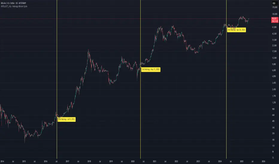
KillZones & Sessions [TradingFinder] Volume | Asia, London & NY🔵 Introduction
🟣 Session
The forex market operates 24 hours a day, 5 days a week, with only Saturdays and Sundays being off; traders often focus on one of the forex trading sessions instead of trying to trade in all markets 24 hours a day.
Trading sessions are time intervals during which a specific financial market is active and trades are conducted. The Asia, London, and New York sessions are the most important trading sessions throughout the 24-hour period, during which a significant amount of money and liquidity enters the market.
🟣 Kill Zone
Traders in financial markets profit from the difference between the price at which they buy or sell and the current market price. Traders have different time horizons for trading.
Among these, some traders engage in daily or even hourly trading and must operate during times when the market has desirable trading volumes and significant price movements.
Kill zones are segments of a session with higher trading volumes and price fluctuations compared to the rest of the session.
🔵 How to Use
🟣 Session Time
The "Asia Session" consists of two sessions: "Sydney" and "Tokyo." The beginning of this session, according to the "UTC" time zone, is at 23:00 and ends at 06:00. Similarly, the beginning of the "Asia KillZone," according to the "UTC" time zone, is at 23:00, and it ends at 03:55.
The "London Session" consists of two sessions: "Frankfurt" and "London." The beginning of this session, according to the "UTC" time zone, is at 07:00, and it ends at 14:25. Similarly, the beginning of the "London KillZone," according to the "UTC" time zone, is at 07:00, and it ends at 09:55.
The beginning of the "New York am" session, according to the "UTC" time zone, is at 14:30, and it ends at 19:25. Similarly, the beginning of the "New York am KillZone," according to the "UTC" time zone, is at 14:30, and it ends at 16:55.
The beginning of the "New York pm" session, according to the "UTC" time zone, is at 19:30, and it ends at 22:55. Similarly, the beginning of the "New York pm KillZone," according to the "UTC" time zone, is at 19:30, and it ends at 20:55.
Important : To prevent session overlap, the working hours of each session have slightly changed.
🔵 Features
🟣 Simultaneous Session and Kill Zone
With this indicator, you can simultaneously view the kill zone and session. High and low lines are used to indicate sessions, while filled areas with color represent kill zones. If you do not want to see kill zones, you can turn off the display settings.
🟣 Candle, Time, and Volume
Using the "More Info" feature, you can see the number of candles, elapsed time, and traded volume within the colored filled area.
🔵 Settings
•Show More Info: To display "More Info," you need to turn on this feature and turn it off whenever you don't need it.
• You can also customize these settings for each session separately :
o Display or hide session.
o Choose session color.
o Set session time range.
o Display or hide kill zone.
o Set kill zone time range.