Ribbit RangesBounce Around Multiple
(Open, High, Low, Close) Ranges
On Pre/Post Market & (Daily, Weekly,
Monthly, Yearly) Sessions With
Meticulous Lines, Labels, Tooltips,
Colors, Custom Ideas, and Alerts.
Sessions Use Two Step Incremental Values
Default Value: (1) Shows Two Previous
(O, H, L, C); Increasing Value Swaps
Sessions With Next Two Ranges.
⬛️ KEY WORDS:
🟢 Crossover | 🔴 Crossunder
📗 High | 📕 Low
📔 Open | 📓 Close
🥇 First Idea | 🥈 Second Idea
🥉 Third Idea | 🎖️ Fourth Idea
🟥 ALERTS:
Default Option: (Per Bar)
Alerts Once Conditions Are Met
(Bar Close) Alerts When Bar Closes
Default Option: (Reg)
Alerts During Regular Market
Trading Hours, (0930-1600)
(Ext) Alerts During Extended
Market Hours, (1600-0930)
(24/7) Alerts All Day
Optional Preferences:
Regular Alerts - Stocks
Extended Alerts - Futures
24/7 Alerts - Crypto
🟧 RANGES:
Default Value: (1)
Incremental Range Value, Increasing Value
Swaps Sessions With the Next Two Ranges
(✓) Swap Ranges?
Pre/Post Market High/Lows,
1-2 Day High/Lows, 1-2 Week High/Lows,
1-2 Month High/Lows, 1-2 Year High/Lows
( ) Swap Ranges?
Pre/Post Market Open/Close,
1-2 Day Open/Close, 1-2 Week Open/Close,
1-2 Month Open/Close, 1-2 Year Open/Close
🟨 EXAMPLES:
Default Range:
🟢 | 📗 Pre Market High (PRE) | 4600.00
🔴 | 📕 Post Market Low (POST) | 420.00
Optional: (Open)
🟢 | 📔 Post Market Open (POST) | 4400.00
Optional: (Close)
🔴 | 📓 Pre Market Close (PRE) | 430.00
Default Range Value: (1)
🔴 | 📗 1 Day High (1DH) | 460.00
Next Range Value: (3)
🟢 | 📕 4 Day Low (4DL) | 420.00
Optional: (Open)
🔴 | 📔 2 Day Open (2DO) | 440.00
Optional: (Close)
🟢 | 📓 3 Day Close (3DC) | 430.00
Default Range Value: (5)
🟢 | 📗 5 Week High (5WH) | 460.00
Next Range Value: (7)
🔴 | 📕 8 Week Low (8WL) | 420.00
Optional: (Open)
🔴 | 📔 7 Week Open (7WO) | 4400.00
Optional: (Close)
🟢 | 📓 6 Week Close (6WC) | 430.00
Default Range Value: (9)
🔴 | 📗 9 Month High (9MH) | 460.00
Next Range Value: (11)
🟢 | 📕 12 Month Low (12ML) | 420.00
Optional: (Open)
🟢 | 📔 11 Month Open (11MO) | 4400.00
Optional: (Close)
🔴 | 📓 10 Month Close (10MC) | 430.00
Default Range Value: (13)
🟢 | 📗 13 Year High (13YH) | 460.00
Next Range Value: (15)
🟢 | 📕 16 Year Low (16YL) | 420.00
Optional: (Open)
🔴 | 📔 15 Year Open (15YO) | 4400.00
Optional: (Close)
🔴 | 📓 14 Year Close (14YC) | 430.00
🟩 COLORS:
(✓) Swap Colors?
Text Color Is Shown Using
Background Color
( ) Swap Colors?
Background Color Is Shown
Using Text Color
🟦 IDEAS:
(✓) Show Ideas?
Plots Four Ideas With Custom Lines
and Labels; Ideas Are Based Around
Post-It Note Reminders with Alerts
Suggestions For Text Ideas:
Take Profit, Stop Loss, Trim, Hold,
Long, Short, Bounce Spot, Retest,
Chop, Support, Resistance, Buy, Sell
🟪 EXAMPLES:
Default Value: (5)
Shows the Custom Value For
Lines, Labels, and Alerts
Default Text: (🥇)
Shown On First Label and
Message Appearing On Alerts
Alert Shows: 🟢 | 🥇 | 5.00
Default Value: (10)
Shows the Custom Value For
Lines, Labels, and Alerts
Default Text: (🥈)
Shown On Second Label and
Message Appearing On Alerts
Alert Shows: 🔴 | 🥈 | 10.00
Default Value: (50)
Shows the Custom Value For
Lines, Labels, and Alerts
Default Text: (🥉)
Shown On Third Label and
Message Appearing On Alerts
Alert Shows: 🟢 | 🥉 | 50.00
Default Value: (100)
Shows the Custom Value For
Lines, Labels, and Alerts
Default Text: (🎖️)
Shown On Fourth Label and
Message Appearing On Alerts
Alert Shows: 🔴 | 🎖️ | 100.00
⬛️ REFERENCES:
Pre-market Highs & Lows on regular
trading hours (RTH) chart
By Twingall
Previous Day Week Highs & Lows
By Sbtnc
Screener for 40+ instruments
By QuantNomad
Daily Weekly Monthly Yearly Opens
By Meliksah55
Cerca negli script per "豪24配债"
VIX HeatmapVIX HeatMap
Instructions:
- To be used with the S&P500 index (ES, SPX, SPY, any S&P ETF) as that's the input from where the CBOE calculates and measures the VIX. Can also be used with the Dow Jones, Nasdaq, & Nasdaq100.
Description:
- Expected Implied Volatility regime simplified & visualized. Know if we are in a high, medium, or low volatility regime, instantly.
- Ranges from Hot to Cold: The hotter the heat-map, the higher the implied volatility and fear & vice versa.
- The VIX HeatMap, color-maps important VIX levels (7 in this case) in measuring volatility for day trading & swing trading.
Using the VIX HeatMap:
- A LOW level volatility environment: Represented by "cooler" colors (Blue & White) depicts that the level of volatility and fear is low. Percentage moves on the index level are going to be tame and less volatile more often than not. Low fear = low perceived risk.
- A MEDIUM level volatility environment: Represented by "warmer" colors (Green & Yellow) depicts that the markets are transitioning from a calmer period or from a more fearful period. Market volatility here will be higher and provide more volatile swings in price.
- A HIGH level volatility environment: Represented by "hotter" colors (Orange, Red, & Purple) depicts that the markets are very fearful at the moment and will have big swings in both directions. Historically, extreme VIX levels tend to coincide with bottoms but are in no way predictive of the exact timing as the volatile moves can continue for an extended period of time.
- Transitioning between the 7 VIX Zones: Each and every one of these specific VIX zone levels is important.
1. Extreme low: <16
2. Low: 16 to 20
3. Normal: 20 to 24
4. Medium: 24 to 28
5. Med-High: 28 to 32
6. High: 32 to 36
7. Extreme high: >36
- These VIX levels in particular measure volatility changes that have a major impact on switching between smaller time frames and measuring depths of a sell move and vice versa. Each level also behaves as its own support & resistance level in terms of taking a bit of effort to switch regimes, and aids in identifying and measuring the potential depth of pullbacks in bull markets and bounces in bear markets to reveal reversal points.
- Examples of VIX level supports depicted on the chart marked with arrows. From left to right:
1. March 10th: Markets jumped 2 volatility levels in 2 days. The fluctuations from blue to yellow to green where a sign that price action would reverse from the selloff.
2. March 28th: As soon as we move from green to the blue VIX level (<20), markets began to rally and only ended when the volatility level moved sub VIX 16 (white).
3. May 4th & 24th: Next we see the 2 dips where volatility levels went from blue to green (VIX > 20), marked bottoms and reversed higher.
4. June 1st: We see a change in VIX regime yet again into lower VIX level and markets rocket higher.
Knowing the current VIX regime is a very important tool and aid in trading, now easily visualized.

Expected VolatilityExpected Volatility
Hello and welcome to my first indicator! I'm publishing this indicator as free to use and modify because I think it's a great place to learn and I hope I can teach you something.
There are some terms which you need to understand before I begin explaining this indicator and what it does for you:
Daily Settlement - The price at which a market closes when the trading day closes (RTH or Regular Trading Hours close)
Standard Deviation - A measure in statistics that declares how far away a data point is from the mean when compared with all the data points before it to an extent
Now for the history behind this indicator:
Rule of 16. This goes back to the VIX, or S&P 500 volatility index. The idea behind the volatility index is to determine what magnitude of movement could be expected from the market the following day based on recent movement. The rule of 16 is an easier way to refer to the square root of the number of trading days in a year. There are 252 trading days in a year and the square root of 252 is approximately 15.87. We estimate it to be 16 because it's easier to talk about when it's easier to say and therefore easier to remember.
The relevance of this rule is that when the VIX is at 16, we can expect a market movement of 1% or so unless some special circumstances overrule this estimate. To get the expected market movement, we take 16 and divide by 16 and get 1, or 1%. If the VIX is trading at 24, we get 24/16 or 1.5 which is 1.5% movement. This indicator seeks to simplify the math and lay it out in a visual way to show the highest probability of range the market is expected to trade.
Thanks for taking the time to read my description, I hope you like my indicator.
Special thanks to my trading friends and coaches for helping me complete this indicator.
Take Session High/Low Alert [MsF]Japanese below / 日本語説明は英文の後にあります。
-------------------------
This indicator that displays High/Low lines for each session. The Key Levels of each session can be visually recognized, which is useful for PD Array analysis. You can display the last 3 days. Based on trinity by ICT.
The biggest feature is that the color shape of the line changes when reaching High/Low. Of course, you can also set alerts.
Unreached High/Low lines can be extended to the right. hides all timeframes over 1 hour. (alert is alive)
You can choose 4 sessions. If you only want to use 3 sessions, you can do that by setting the same session time for 2 of the 4 session settings.
About Parameter Settings
Session Time: Please set it to be a 24-hour cycle. You can also specify the time zone. The default is NY time.
Basis/Other color: The first time specified in "Session Time" in this indicator's parameter is the "Basis color". "Other color" is a line other than that.
Enable Time Lines: You can turn on/off the display of vertical lines.
High/Low color: High/Low line setting that has not been reached.
Taken color: High/Low line setting that has already been reached.
Extend Lines: Allows unreached High/Low lines to be extended to the right in the chart.
-------------------------
セッションごとのHigh/Lowをライン表示するインジケーターです。
過去約3日分を表示することができます。
最大の特徴はHigh/Low到達時にラインの色形が変わることです。もちろんアラート設定も可能です。
未到達のHigh/Lowラインは右側に延長することができます。
チャート表示がビジーとなる為、1時間を超える時間足ではすべて非表示とする仕様です。(アラートは生きてます)
セッションは4つ指定できます。
もしセッションを3つのみ使用したい場合は、4つのセッション設定の内2つに同じセッション時間を設定することで実現可能です。
■パラメータ設定
Session Time:24時間周期となるように設定してください。またタイムゾーンが指定できます。デフォルトはNY timeです。
Basis/Other color:パラメータの"Session Time"にて一番最初に指定した時間が基準=Basisとなります。Otherはそれ以外のラインとなります。
Enable Time Lines:垂直ラインの表示ON/OFFが可能です。
High/Low color:未到達のHigh/Lowライン設定となります。
Taken color:到達済みのHigh/Lowライン設定となります。
Extend Lines:未到達のHigh/Lowラインを右に延長できます。
Trading ChannelTrading Channel aims to be a canvas on which to develop any strategy that the user feels comfortable with.
The greatest utility of the script lies in the fact that it plots a channel over the price action, as a support and resistance pivot, within which the price action develops.
It is a script of maximum simplicity in concept and development, but at the same time presents robust support to the price action and a quick visual aid complementary to any indicators that the user works with, feels comfortable with, and uses as a basis for their strategies.
The script includes the following features (most of them disabled by default, available for potential use without the need to add additional indicators):
Fast SMA
Medium SMA
Slow SMA (disabled)
Fast EMA (disabled)
Medium EMA (disabled)
Slow EMA (disabled)
Pivot
Pivot SMA
P Multiplier
Set of resistance and support pivots according to the studies of John L. Person (R3, R2, R1, S1, S2, S3 and midpoints) (disabled by default)
Channel for the current time period in use
Channels for extended time periods (disabled by default)
Various trend, momentum, and overbought/oversold indicating labels (note that the calculations for their representation are based on SMA's even though EMA's are visualized).
SMA's/EMA's
Both are available as both are used as basic indicators for different types of strategies. The default selection of SMA's in this case is based on the fact that the script development is largely based on the studies shared by John L. Person in the area of pivots and by Bill Williams in the area of fractals. Note also that for that same reason the various trend, momentum, and overbought/oversold indicating labels are calculated based on them.
Set of resistance and support pivots
They are included as a consultation tool especially for the higher time periods. They can be used to mark the most interesting supports/resistances and not lose sight of them while operating in lower time periods. Marking monthly, weekly, and daily pivots can be very useful. Additionally, marking S1 and R2 for bullish trends, S1 and R1 for ranges, and S2 and R1 for bearish trends can provide an even more precise framework to work on.
P Multiplier
It is set by default at 4, and is the basis for being able to consider during the use of a specific time frame, the price action with respect to higher time frames. It is the multiplier used for the generation of channels for extended time periods.
Channel for the current time period in use
It is a channel formed by the maximum and minimum closing of the last 21 periods. This value is modifiable and its adjustment depends on the asset under study. 24/7 markets show good results with this adjustment (in the case of BTC really good).
This channel represents a pivot in the form of a yellow middle line, with its support and resistance extremes on the upper green and lower red lines. The same green and red lines, referenced this time to the maximum, are added and serve as possible stop-loss marks.
Channels for extended time periods
Enabling the maximum and minimum channels for extended periods can provide a better idea of the price situation (it is recommended to disable the channel in use and enable the upper one for consultation, it provides a better vision).
Identifying labels:
Following a summary explanation for possible long entries, the same but opposite should be considered for possible short entries:
Small green arrow under candle: indicates possible upward trend (pivot above pivot SMA)
Large green arrow under candle: indicates upward trend (pivot above pivot SMA and above fast SMA)
Green triangle over candle: indicates channel breakout, possible upward momentum (represented as a fractal as its concept is the same)
Green/red arrows at the bottom of the chart: intended to confirm the validity of a signal (should doubt green indications with red lower arrow and vice versa)
Green/red dots at the bottom of the chart: red represents areas of strong resistance and green signals of strong support (with red dots, proceed with caution despite green signals, and vice versa)
Comments
It is emphasized that the basic and most useful functionality of this script is to provide a reliable base on which to develop any strategy, as a framework for working.
If the identifying labels are used, it should be taken into account that the earliest will always be the most reliable and valuable, but their confirmation will always depend on the user's strategy.
Its use in conjunction with the "Pivot Position for Trading Channel" indicator can serve as a base for the development of different strategies, by providing indication of the relative position of the price within the channel.
This script is just a consultation tool with didactic goals, it should not be used as an investment recommendation and the information provided should not be relied upon as such.
------------------------
Trading Channel pretende ser un lienzo sobre el que desarrollar cualquiera que sea la estrategia con la que el usuario se sienta más cómodo.
La mayor utilidad del script radica en que se traza sobre la acción del precio un canal, a modo de pivotes de soporte y resistencia, dentro del cual se desarrolla la acción del precio.
Se trata de un script de máxima sencillez en concepto y desarrollo, pero que a la vez presenta un soporte robusto a la acción del precio y una ayuda rápida visual complementaria a cualquieras que sean los indicadores con los que el usuario trabaje, se sienta más cómodo y utilice como base de sus estrategias.
El script incluye las siguientes funcionalidades (la mayoría desactivadas por defecto, disponibles para su potencial uso sin necesidad de añadir indicadores adicionales):
- SMA rápida
- SMA media
- SMA lenta (desactivada)
- EMA rápida (desactivada)
- EMA media (desactivada)
- EMA lenta (desactivada)
- Pivote
- SMA de pivote
- Multiplicador de P
- Conjunto de pivotes resistencia y soporte de acuerdo a los estudios de John L. Person (R3, R2, R1, S1, S2, S3 y puntos medios) (desactivados por defecto)
- Canal para el periodo temporal en uso
- Canales para periodos temporales extendidos (desactivados por defecto)
- Diversas etiquetas indicativas de cambios de tendencia, de impulso y de sobrecompra y sobreventa (nótese que los cálculos para su representación están basados en SMA's aunque se visualicen EMA's).
SMA's/EMA's
Ambas disponibles pues tanto unas como otras son utilizadas como indicadores básicos para diferentes tipos de estrategias. La selección de SMA's por defecto en este caso se basa en que las bases para desarrollo del script son en gran medida los estudios compartidos por John L. Person en el área de pivotes y de Bill Williams en el área de los fractales. Nótese también que por esa misma razón las diversas etiquetas indicativas de cambios de tendencia, impulso y sobrecompra/sobreventa se calculan en base a ellas.
Conjunto de pivotes resistencia y soporte
Se incluyen como herramienta de consulta sobre todo para los periodos temporales más altos. Pueden utilizarse para marcar los soportes/resistencias de más interés y no perderlos de vista mientras se opera en periodos de tiempo más bajos. De acuerdo a los estudios de John L. Person, marcarse los pivotes mensuales, semanales y diarios puede resultar de mucha utilidad. Adicionalmente, marcar S1 y R2 para tendencias alcistas, S1 y R1 para rangos, y S2 y R1 para tendencias bajistas puede proporcionar un marco aún más preciso sobre el que trabajar.
Multiplicador de p
Está fijado por defecto en 4, y es la base para poder considerar durante el uso de una franja temporal concreta, la acción del precio respecto a franjas temporales superiores. Es el multiplicador utilizado para la generación de los canales para periodos temporales extendidos.
Canal para el periodo temporal en uso
Se trata de un canal conformado por los cierres máximos y mínimos de los últimos 21 periodos. Este valor es modificable y su ajuste depende del activo en estudio. Mercados 24/7 muestran buenos resultados con este ajuste (en el caso de BTC realmente buenos).
Este canal representa en cierta manera un pivote en forma de línea intermedia amarilla, con sus extremos de soporte y resistencia en las líneas verdes superior y roja inferior. Se añaden las mismas líneas verdes y rojas, referenciadas esta vez a los máximos, que sirven como posibles marcas de stop-loss.
Canales para periodos temporales extendidos
Habilitar los máximos y mínimos de canales de periodos extendidos puede proporcionar una mejor idea de la situación del precio (se recomienda deshabilitar el canal en uso y habilitar el superior para consulta, proporciona una mejor visión).
Etiquetas identificativas:
A continuación explicación resumida para posibles entradas en largo, lo mismo pero de modo opuesto debería considerarse para posibles entradas en corto:
Flecha verde pequeña bajo vela: indica inicio de tendencia en alza (pivote por encima de SMA de pivote y ambos por encima de SMA rápida)
Flecha verde grande bajo vela: indica tendencia en alza (pivote por encima de SMA de pivote y ambos por encima de SMA rápida y media)
Triángulo verde sobre vela: indica rotura de canal, posible impulso al alza (representado a modo de fractal pues su concepto es el mismo)
Flechas verdes/rojas a pie de gráfico: pretenden confirmar la validez de una señal (debería dudarse de las indicaciones verdes con flecha inferior roja y viceversa)
Puntos verdes/rojos a pie de gráfico: los rojos representan áreas de fuerte resistencia y los verdes de fuerte soporte (con puntos rojos, proceder con cautela pese a señales verdes, y viceversa)
Comentarios
Se insiste en que la funcionalidad básica y de mayor utilidad de este script es proporcionar una base confiable sobre la que desarrollar cualquier estrategia, a modo de marco de trabajo.
Si se hace uso de las etiquetas identificativas, debe tenerse en cuenta que las más prematuras siempre serán las más confiables y valiosas, pero que su confirmación siempre dependerá de la estrategia por parte del usuario.
Su uso en conjunción al indicador "Pivot Position for Trading Channel" puede servir de base para el desarrollo de diferentes estrategias, al proporcionar indicación de la posición relativa del precio dentro del canal.
Este script es solo una herramienta de consulta con objetivos didácticos, no debe ser utilizado como recomendación de inversión y no se debe confiar en ella como tal.
dmn's ICT ToolkitThis is my quality of life indicator for forex trading using the methods and concepts of ICT.
The idea is to automate marking up important price levels and times of the day instead of doing it manually every day.
Killzones
Marks the most volatile times of the day on the chart, during which the intraday high/low usually takes place.
Particularly impactful when there's news released during these times.
London Open (02:00-05:00 EST)
New York Open (08:30-11:00 EST)
London Close (10:00-11:30 EST)
True Day delineation
Vertical line at the start of the "true day" (00:00 EST), start of the algorithmic trading day and aids in visualizing the intraday direction.
New York midnight price level
Noteworthy price level at the start of the "true day".
This price level is referenced by the interbank trading algorithms during the day. Buy below it on bullish days, sell above it on bearish days.
Daily open price level
Reference level for optimal trade entries. Buy below it on bullish days, sell above it on bearish days.
Central Banks Dealers Range (CBDR) (14:00-20:00 EST) &
Central Banks Dealers Flout (CBDF) (15:00-24:00 EST) &
Asian Range (AR) (20:00-24:00 EST)
The standard deviation lines available are used to make predictions for short-term future highs/lows when the CBDR and AR are smaller than 40 pips.
Trade them by looking for 5/15min key levels that converge with the projection levels.
X days Average Daily Range (ADR)
Default to 5 days back, gives an idea of how much movement to expect intraday when the ADR high/low is converging with CBDR/CBDF/AR standard deviations.
Current Daily Range (CDR)
Used for comparison against the ADR to help determine if there's enough intraday range left to enter a trade.
Dynamically changes color based on percentage of the ADR. Green below 50% of ADR, orange between 50 and 100%, red when CDR exceeds ADR.
All of the above are used in conjunction with each other and higher timeframe levels of importance to find entries and target.
Note: Preferably use New York's time zone for your charts.

Day Trading Booster by DGTTiming when day trading can be everything
In Stock markets typically more volatility (or price activity) occurs at market opening and closings
When it comes to Forex (foreign exchange market), the world’s most traded market, unlike other financial markets, there is no centralized marketplace, currencies trade over the counter in whatever market is open at that time, where time becomes of more importance and key to get better trading opportunities. There are four major forex trading sessions, which are Sydney , Tokyo , London and New York sessions
Forex market is traded 24 hours a day, 5 days a week across by banks, institutions and individual traders worldwide, but that doesn’t mean it’s always active the entire day. It may be very difficult time trying to make money when the market doesn’t move at all. The busiest times with highest trading volume occurs during the overlap of the London and New York trading sessions, because U.S. dollar (USD) and the Euro (EUR) are the two most popular currencies traded. Typically most of the trading activity for a specific currency pair will occur when the trading sessions of the individual currencies overlap. For example, Australian Dollar (AUD) and Japanese Yen (JPY) will experience a higher trading volume when both Sydney and Tokyo sessions are open
There is one influence that impacts Forex matkets and should not be forgotten : the release of the significant news and reports. When a major announcement is made regarding economic data, currency can lose or gain value within a matter of seconds
Cryptocurrency markets on the other hand remain open 24/7, even during public holidays
Until 2021, the Asian impact was so significant in Cryptocurrency markets but recent reasearch reports shows that those patterns have changed and the correlation with the U.S. trading hours is becoming a clear evolving trend.
Unlike any other market Crypto doesn’t rest on weekends, there’s a drop-off in participation and yet algorithmic trading bots and market makers (or liquidity providers) can create a high volume of activity. Never trust the weekend’ is a good thing to remind yourself
One more factor that needs to be taken into accout is Blockchain transaction fees, which are responsive to network congestion and can change dramatically from one hour to the next
In general, Cryptocurrency markets are highly volatile, which means that the price of a coin can change dramatically over a short time period in either direction
The Bottom Line
The more traders trading, the higher the trading volume, and the more active the market. The more active the market, the higher the liquidity (availability of counterparties at any given time to exit or enter a trade), hence the tighter the spreads (the difference between ask and bid price) and the less slippage (the difference between the expected fill price and the actual fill price) - in a nutshell, yield to many good trading opportunities and better order execution (a process of filling the requested buy or sell order)
The best time to trade is when the market is the most active and therefore has the largest trading volume, trading all day long will not only deplete a trader's reserves quickly, but it can burn out even the most persistent trader. Knowing when the markets are more active will give traders peace of mind, that opportunities are not slipping away when they take their eyes off the markets or need to get a few hours of sleep
What does the Day Trading Booster do?
Day Trading Booster is designed ;
- to assist in determining market peak times, the times where better trading opportunities may arise
- to assist in determining the probable trading opportunities
- to help traders create their own strategies. An example strategy of when to trade or not is presented below
For Forex markets specifically includes
- Opening channel of Asian session, Europien session or both
- Opening price, opening range (5m or 15m) and day (session) range of the major trading center sessions, including Frankfurt
- A tabular view of the major forex markets oppening/closing hours, with a countdown timer
- A graphical presentation of typically traded volume and various forext markets oppening/clossing events (not only the major markets but many other around the world)
For All type of markets Day Trading Booster plots
- Day (Session) Open, 5m, 15m or 1h Opening Range
- Day (Session) Referance Levels, based on Average True Range (ATR) or Previous Day (Session) Range (PH - PL)
- Week and Month Open
Day Trading Booster also includes some of the day trader's preffered indicaotrs, such as ;
- VWAP - A custom interpretaion of VWAP is presented here with Auto, Interactive and Manual anchoring options.
- Pivot High/Low detection - Another custom interpretation of Pivot Points High Low indicator.
- A Moving Average with option to choose among SMA, EMA, WMA and HMA
An example strategy - Channel Bearkout Strategy
When day trading a trader usually monitors/analyzes lower timeframe charts and from time to time may loose insight of what really happens on the market from higher time porspective. Do not to forget to look at the larger time frame (than the one chosen to trade with) which gives the bigger picture of market price movements and thus helps to clearly define the trend
Disclaimer : Trading success is all about following your trading strategy and the indicators should fit within your trading strategy, and not to be traded upon solely
The script is for informational and educational purposes only. Use of the script does not constitutes professional and/or financial advice. You alone the sole responsibility of evaluating the script output and risks associated with the use of the script. In exchange for using the script, you agree not to hold dgtrd TradingView user liable for any possible claim for damages arising from any decision you make based on use of the script

lower_tf█ OVERVIEW
This library is a Pine programmer’s tool containing functions to help those who use the request.security_lower_tf() function. Its `ltf()` function helps translate user inputs into a lower timeframe string usable with request.security_lower_tf() . Another function, `ltfStats()`, accumulates statistics on processed chart bars and intrabars.
█ CONCEPTS
Chart bars
Chart bars , as referred to in our publications, are bars that occur at the current chart timeframe, as opposed to those that occur at a timeframe that is higher or lower than that of the chart view.
Intrabars
Intrabars are chart bars at a lower timeframe than the chart's. Each 1H chart bar of a 24x7 market will, for example, usually contain 60 intrabars at the LTF of 1min, provided there was market activity during each minute of the hour. Mining information from intrabars can be useful in that it offers traders visibility on the activity inside a chart bar.
Lower timeframes (LTFs)
A lower timeframe is a timeframe that is smaller than the chart's timeframe. This framework exemplifies how authors can determine which LTF to use by examining the chart's timeframe. The LTF determines how many intrabars are examined for each chart bar; the lower the timeframe, the more intrabars are analyzed.
Intrabar precision
The precision of calculations increases with the number of intrabars analyzed for each chart bar. As there is a 100K limit to the number of intrabars that can be analyzed by a script, a trade-off occurs between the number of intrabars analyzed per chart bar and the chart bars for which calculations are possible.
█ `ltf()`
This function returns a timeframe string usable with request.security_lower_tf() . It calculates the returned timeframe by taking into account a user selection between eight different calculation modes and the chart's timeframe. You send it the user's selection, along with the text corresponding to the eight choices from which the user has chosen, and the function returns a corresponding LTF string.
Because the function processes strings and doesn't require recalculation on each bar, using var to declare the variable to which its result is assigned will execute the function only once on bar zero and speed up your script:
var string ltfString = ltf(ltfModeInput, LTF1, LTF2, LTF3, LTF4, LTF5, LTF6, LTF7, LTF8)
The eight choices users can select from are of two types: the first four allow a selection from the desired amount of chart bars to be covered, the last four are choices of a fixed number of intrabars to be analyzed per chart bar. Our example code shows how to structure your input call and then make the call to `ltf()`. By changing the text associated with the `LTF1` to `LTF8` constants, you can tailor it to your preferences while preserving the functionality of `ltf()` because you will be sending those string constants as the function's arguments so it can determine the user's selection. The association between each `LTFx` constant and its calculation mode is fixed, so the order of the arguments is important when you call `ltf()`.
These are the first four modes and the `LTFx` constants corresponding to each:
Covering most chart bars (least precise) — LTF1
Covers all chart bars. This is accomplished by dividing the current timeframe in seconds by 4 and converting that number back to a string in timeframe.period format using secondsToTfString() . Due to the fact that, on premium subscriptions, the typical historical bar count is between 20-25k bars, dividing the timeframe by 4 ensures the highest level of intrabar precision possible while achieving complete coverage for the entire dataset with the maximum allowed 100K intrabars.
Covering some chart bars (less precise) — LTF2
Covering less chart bars (more precise) — LTF3
These levels offer a stepped LTF in relation to the chart timeframe with slightly more, or slightly less precision. The stepped lower timeframe tiers are calculated from the chart timeframe as follows:
Chart Timeframe Lower Timeframe
Less Precise More Precise
< 1hr 1min 1min
< 1D 15min 1min
< 1W 2hr 30min
> 1W 1D 60min
Covering the least chart bars (most precise) — LTF4
Analyzes the maximum quantity of intrabars possible by using the 1min LTF, which also allows the least amount of chart bars to be covered.
The last four modes allow the user to specify a fixed number of intrabars to analyze per chart bar. Users can choose from 12, 24, 50 or 100 intrabars, respectively corresponding to the `LTF5`, `LTF6`, `LTF7` and `LTF8` constants. The value is a target; the function will do its best to come up with a LTF producing the required number of intrabars. Because of considerations such as the length of a ticker's session, rounding of the LTF to the closest allowable timeframe, or the lowest allowable timeframe of 1min intrabars, it is often impossible for the function to find a LTF producing the exact number of intrabars. Requesting 100 intrabars on a 60min chart, for example, can only produce 60 1min intrabars. Higher chart timeframes, tickers with high liquidity or 24x7 markets will produce optimal results.
█ `ltfStats()`
`ltfStats()` returns statistics that will be useful to programmers using intrabar inspection. By analyzing the arrays returned by request.security_lower_tf() in can determine:
• intrabarsInChartBar : The number of intrabars analyzed for each chart bar.
• chartBarsCovered : The number of chart bars where intrabar information is available.
• avgIntrabars : The average number of intrabars analyzed per chart bar. Events like holidays, market activity, or reduced hours sessions can cause the number of intrabars to vary, bar to bar.
The function must be called on each bar to produce reliable results.
█ DEMONSTRATION CODE
Our example code shows how to provide users with an input from which they can select a LTF calculation mode. If you use this library's functions, feel free to reuse our input setup code, including the tooltip providing users with explanations on how it works for them.
We make a simple call to request.security_lower_tf() to fetch the close values of intrabars, but we do not use those values. We simply send the returned array to `ltfStats()` and then plot in the indicator's pane the number of intrabars examined on each bar and its average. We also display an information box showing the user's selection of the LTF calculation mode, the resulting LTF calculated by `ltf()` and some statistics.
█ NOTES
• As in several of our recent publications, this script uses secondsToTfString() to produce a timeframe string in timeframe.period format from a timeframe expressed in seconds.
• The script utilizes display.data_window and display.status_line to restrict the display of certain plots.
These new built-ins allow coders to fine-tune where a script’s plot values are displayed.
• We implement a new recommended best practice for tables which works faster and reduces memory consumption.
Using this new method, tables are declared only once with var , as usual. Then, on bar zero only, we use table.cell() calls to populate the table.
Finally, table.set_*() functions are used to update attributes of table cells on the last bar of the dataset.
This greatly reduces the resources required to render tables. We encourage all Pine Script™ programmers to do the same.
Look first. Then leap.
█ FUNCTIONS
The library contains the following functions:
ltf(userSelection, choice1, choice2, choice3, choice4, choice5, choice6, choice7, choice8)
Selects a LTF from the chart's TF, depending on the `userSelection` input string.
Parameters:
userSelection : (simple string) User-selected input string which must be one of the `choicex` arguments.
choice1 : (simple string) Input selection corresponding to "Least precise, covering most chart bars".
choice2 : (simple string) Input selection corresponding to "Less precise, covering some chart bars".
choice3 : (simple string) Input selection corresponding to "More precise, covering less chart bars".
choice4 : (simple string) Input selection corresponding to "Most precise, 1min intrabars".
choice5 : (simple string) Input selection corresponding to "~12 intrabars per chart bar".
choice6 : (simple string) Input selection corresponding to "~24 intrabars per chart bar".
choice7 : (simple string) Input selection corresponding to "~50 intrabars per chart bar".
choice8 : (simple string) Input selection corresponding to "~100 intrabars per chart bar".
Returns: (simple string) A timeframe string to be used with `request.security_lower_tf()`.
ltfStats()
Returns statistics about analyzed intrabars and chart bars covered by calls to `request.security_lower_tf()`.
Parameters:
intrabarValues : (float [ ]) The ID of a float array containing values fetched by a call to `request.security_lower_tf()`.
Returns: A 3-element tuple: [ (series int) intrabarsInChartBar, (series int) chartBarsCovered, (series float) avgIntrabars ].

Jurik Composite Fractal Behavior (CFB) on EMA [Loxx]Jurik Composite Fractal Behavior (CFB) on EMA is an exponential moving average with adaptive price trend duration inputs. This purpose of this indicator is to introduce the formulas for the calculation Composite Fractal Behavior. As you can see from the chart above, price reacts wildly to shifts in volatility--smoothing out substantially while riding a volatility wave and cutting sharp corners when volatility drops. Notice the chop zone on BTC around August 2021, this was a time of extremely low relative volatility.
This indicator uses three previous indicators from my public scripts. These are:
JCFBaux Volatility
Jurik Filter
Jurik Volty
The CFB is also related to the following indicator
Jurik Velocity ("smoother moment")
Now let's dive in...
What is Composite Fractal Behavior (CFB)?
All around you mechanisms adjust themselves to their environment. From simple thermostats that react to air temperature to computer chips in modern cars that respond to changes in engine temperature, r.p.m.'s, torque, and throttle position. It was only a matter of time before fast desktop computers applied the mathematics of self-adjustment to systems that trade the financial markets.
Unlike basic systems with fixed formulas, an adaptive system adjusts its own equations. For example, start with a basic channel breakout system that uses the highest closing price of the last N bars as a threshold for detecting breakouts on the up side. An adaptive and improved version of this system would adjust N according to market conditions, such as momentum, price volatility or acceleration.
Since many systems are based directly or indirectly on cycles, another useful measure of market condition is the periodic length of a price chart's dominant cycle, (DC), that cycle with the greatest influence on price action.
The utility of this new DC measure was noted by author Murray Ruggiero in the January '96 issue of Futures Magazine. In it. Mr. Ruggiero used it to adaptive adjust the value of N in a channel breakout system. He then simulated trading 15 years of D-Mark futures in order to compare its performance to a similar system that had a fixed optimal value of N. The adaptive version produced 20% more profit!
This DC index utilized the popular MESA algorithm (a formulation by John Ehlers adapted from Burg's maximum entropy algorithm, MEM). Unfortunately, the DC approach is problematic when the market has no real dominant cycle momentum, because the mathematics will produce a value whether or not one actually exists! Therefore, we developed a proprietary indicator that does not presuppose the presence of market cycles. It's called CFB (Composite Fractal Behavior) and it works well whether or not the market is cyclic.
CFB examines price action for a particular fractal pattern, categorizes them by size, and then outputs a composite fractal size index. This index is smooth, timely and accurate
Essentially, CFB reveals the length of the market's trending action time frame. Long trending activity produces a large CFB index and short choppy action produces a small index value. Investors have found many applications for CFB which involve scaling other existing technical indicators adaptively, on a bar-to-bar basis.
What is Jurik Volty used in the Juirk Filter?
One of the lesser known qualities of Juirk smoothing is that the Jurik smoothing process is adaptive. "Jurik Volty" (a sort of market volatility ) is what makes Jurik smoothing adaptive. The Jurik Volty calculation can be used as both a standalone indicator and to smooth other indicators that you wish to make adaptive.
What is the Jurik Moving Average?
Have you noticed how moving averages add some lag (delay) to your signals? ... especially when price gaps up or down in a big move, and you are waiting for your moving average to catch up? Wait no more! JMA eliminates this problem forever and gives you the best of both worlds: low lag and smooth lines.
Ideally, you would like a filtered signal to be both smooth and lag-free. Lag causes delays in your trades, and increasing lag in your indicators typically result in lower profits. In other words, late comers get what's left on the table after the feast has already begun.
Modifications and improvements
1. Jurik's original calculation for CFB only allowed for depth lengths of 24, 48, 96, and 192. For theoretical purposes, this indicator allows for up to 20 different depth inputs to sample volatility. These depth lengths are
2, 3, 4, 6, 8, 12, 16, 24, 32, 48, 64, 96, 128, 192, 256, 384, 512, 768, 1024, 1536
Including these additional length inputs is arguable useless, but they are are included for completeness of the algorithm.
2. The result of the CFB calculation is forced to be an integer greater than or equal to 1.
3. The result of the CFB calculation is double filtered using an advanced, (and adaptive itself) filtering algorithm called the Jurik Filter. This filter and accompanying internal algorithm are discussed above.

Volume OximeterOVERVIEW
The Volume Oximeter (VOXI) is a technical indicator that gauges the amount of volume currently present in the market, relative to the historical volume that was present before. The purpose of this indicator is to filter out with-trend signals during ranging/non-trending conditions.
CONCEPTS
This indicator assumes that trends are more likely to start during periods of high volume, compared to during periods of low volume. This is because high volume indicates that there are bigger players currently in the market, which is necessary to begin a sustained trending move.
So, to determine whether the current volume is "high", it is compared to an average volume for however number of candles back the user specifies.
If the current volume is greater than the average volume, it is reasonable to assume we are in a high volume period. Thus, this is the ideal time to enter a trending trade due to the assumption that trends are more likely to start during these high volume periods.
The default values in the indicator are designed for use on the daily chart but can be applied to any timeframe.
The default volume lookback period is 259 since there are usually 259 daily candles in a year on Forex daily charts. This means that the average volume will represent the average volume over the past year. This would be 365 on Crypto daily charts, since the Crypto is open 24/7 instead of 24/5). This is what the current volume will be compared to.
The default smoothing lookback period is 10, but this can be adjusted depending on the indicator that's giving you your with-trend signals. After my backtesting, 10 was the best value for my with-trend indicator, so you should do your own testing to see which value works best with your with-trend indicator.
HOW DO I READ THIS INDICATOR?
If the VOXI line is above or equal to zero (indicated by the blue color), the current volume is greater than the historical average volume.
This is a good time to take with-trend signals since high volume is necessary for sustained trending moves to begin.
If the VOXI line is below zero (indicated by the red color), the current volume is less than the historical average volume.
This is a good time to ignore with-trend signals since an absence of volume indicates that there aren't big market participants to participate in a new trending move.

ConditionalAverages█ OVERVIEW
This library is a Pine Script™ programmer’s tool containing functions that average values selectively.
█ CONCEPTS
Averaging can be useful to smooth out unstable readings in the data set, provide a benchmark to see the underlying trend of the data, or to provide a general expectancy of values in establishing a central tendency. Conventional averaging techniques tend to apply indiscriminately to all values in a fixed window, but it can sometimes be useful to average values only when a specific condition is met. As conditional averaging works on specific elements of a dataset, it can help us derive more context-specific conclusions. This library offers a collection of averaging methods that not only accomplish these tasks, but also exploit the efficiencies of the Pine Script™ runtime by foregoing unnecessary and resource-intensive for loops.
█ NOTES
To Loop or Not to Loop
Though for and while loops are essential programming tools, they are often unnecessary in Pine Script™. This is because the Pine Script™ runtime already runs your scripts in a loop where it executes your code on each bar of the dataset. Pine Script™ programmers who understand how their code executes on charts can use this to their advantage by designing loop-less code that will run orders of magnitude faster than functionally identical code using loops. Most of this library's function illustrate how you can achieve loop-less code to process past values. See the User Manual page on loops for more information. If you are looking for ways to measure execution time for you scripts, have a look at our LibraryStopwatch library .
Our `avgForTimeWhen()` and `totalForTimeWhen()` are exceptions in the library, as they use a while structure. Only a few iterations of the loop are executed on each bar, however, as its only job is to remove the few elements in the array that are outside the moving window defined by a time boundary.
Cumulating and Summing Conditionally
The ta.cum() or math.sum() built-in functions can be used with ternaries that select only certain values. In our `avgWhen(src, cond)` function, for example, we use this technique to cumulate only the occurrences of `src` when `cond` is true:
float cumTotal = ta.cum(cond ? src : 0) We then use:
float cumCount = ta.cum(cond ? 1 : 0) to calculate the number of occurrences where `cond` is true, which corresponds to the quantity of values cumulated in `cumTotal`.
Building Custom Series With Arrays
The advent of arrays in Pine has enabled us to build our custom data series. Many of this library's functions use arrays for this purpose, saving newer values that come in when a condition is met, and discarding the older ones, implementing a queue .
`avgForTimeWhen()` and `totalForTimeWhen()`
These two functions warrant a few explanations. They operate on a number of values included in a moving window defined by a timeframe expressed in milliseconds. We use a 1D timeframe in our example code. The number of bars included in the moving window is unknown to the programmer, who only specifies the period of time defining the moving window. You can thus use `avgForTimeWhen()` to calculate a rolling moving average for the last 24 hours, for example, that will work whether the chart is using a 1min or 1H timeframe. A 24-hour moving window will typically contain many more values on a 1min chart that on a 1H chart, but their calculated average will be very close.
Problems will arise on non-24x7 markets when large time gaps occur between chart bars, as will be the case across holidays or trading sessions. For example, if you were using a 24H timeframe and there is a two-day gap between two bars, then no chart bars would fit in the moving window after the gap. The `minBars` parameter mitigates this by guaranteeing that a minimum number of bars are always included in the calculation, even if including those bars requires reaching outside the prescribed timeframe. We use a minimum value of 10 bars in the example code.
Using var in Constant Declarations
In the past, we have been using var when initializing so-called constants in our scripts, which as per the Style Guide 's recommendations, we identify using UPPER_SNAKE_CASE. It turns out that var variables incur slightly superior maintenance overhead in the Pine Script™ runtime, when compared to variables initialized on each bar. We thus no longer use var to declare our "int/float/bool" constants, but still use it when an initialization on each bar would require too much time, such as when initializing a string or with a heavy function call.
Look first. Then leap.
█ FUNCTIONS
avgWhen(src, cond)
Gathers values of the source when a condition is true and averages them over the total number of occurrences of the condition.
Parameters:
src : (series int/float) The source of the values to be averaged.
cond : (series bool) The condition determining when a value will be included in the set of values to be averaged.
Returns: (float) A cumulative average of values when a condition is met.
avgWhenLast(src, cond, cnt)
Gathers values of the source when a condition is true and averages them over a defined number of occurrences of the condition.
Parameters:
src : (series int/float) The source of the values to be averaged.
cond : (series bool) The condition determining when a value will be included in the set of values to be averaged.
cnt : (simple int) The quantity of last occurrences of the condition for which to average values.
Returns: (float) The average of `src` for the last `x` occurrences where `cond` is true.
avgWhenInLast(src, cond, cnt)
Gathers values of the source when a condition is true and averages them over the total number of occurrences during a defined number of bars back.
Parameters:
src : (series int/float) The source of the values to be averaged.
cond : (series bool) The condition determining when a value will be included in the set of values to be averaged.
cnt : (simple int) The quantity of bars back to evaluate.
Returns: (float) The average of `src` in last `cnt` bars, but only when `cond` is true.
avgSince(src, cond)
Averages values of the source since a condition was true.
Parameters:
src : (series int/float) The source of the values to be averaged.
cond : (series bool) The condition determining when the average is reset.
Returns: (float) The average of `src` since `cond` was true.
avgForTimeWhen(src, ms, cond, minBars)
Averages values of `src` when `cond` is true, over a moving window of length `ms` milliseconds.
Parameters:
src : (series int/float) The source of the values to be averaged.
ms : (simple int) The time duration in milliseconds defining the size of the moving window.
cond : (series bool) The condition determining which values are included. Optional.
minBars : (simple int) The minimum number of values to keep in the moving window. Optional.
Returns: (float) The average of `src` when `cond` is true in the moving window.
totalForTimeWhen(src, ms, cond, minBars)
Sums values of `src` when `cond` is true, over a moving window of length `ms` milliseconds.
Parameters:
src : (series int/float) The source of the values to be summed.
ms : (simple int) The time duration in milliseconds defining the size of the moving window.
cond : (series bool) The condition determining which values are included. Optional.
minBars : (simple int) The minimum number of values to keep in the moving window. Optional.
Returns: (float) The sum of `src` when `cond` is true in the moving window.

Volume fight strategyThe Volume fight strategy looks for the predominance of bullish or bearish trading volume on the chart by dividing the trading volume in the bar into 2 parts - "bullish volume" and "bearish volume", and comparing the weighted average values by volume with each other at a given distance.
This strategy is suitable for any instrument (cryptocurrency, Forex, stocks) and is able to work on any TF.
The Volume fight strategy should be used as an auxiliary indicator that tells you who is currently prevailing in the market - " bulls "or"bears".
To configure the strategy , it is necessary to set the range of evaluation of the predominance of bullish or bearish volume (the number of bars, by default-24 bars for TF=1H). The smaller the TF, the higher the range value should be used to filter out false signals.
When there is a predominance of "bulls" on the chart, a green triangle appears (relevant at the close of the bar) and the histogram is highlighted in green, when "bears" appear on the chart, a red triangle appears (relevant at the close of the bar) and the histogram is highlighted in red.
In the strategy settings, there is smoothing to reduce false signals and highlight the flat zone by specifying a percentage, at least which should be the difference between the forces of the "bullish" and "bearish" volume . If the difference between the volume forces is less than the specified one (by default-15%), the zone is considered flat and is displayed in gray on the histogram.
If you set the percentage to zero, the flat zones will not be highlighted, but there will be much more false signals, since the strategy becomes very sensitive when the smoothing percentage decreases.
There is a function-to show the color background of the current trading zone. For" bullish "- green, for" bearish " - red.
In the settings, you can enable the display and use of each signal in the trading zone, not only the initial one, but also each after the flat zone. By default, only the signal of the beginning of the ascending/descending zone is used.
The strategy has alerts for "bullish" and "bearish" movements.
👉Use alerts - "alert() function calls only"
If you have any questions, you can write to me in private messages or by using the contacts in my signature.
----------------------------------------------------
Стратегия Volume fight ищет на графике преобладание бычьего или медвежьего объёма торгов путём разделения торгового объёма в баре на 2 части - "бычий объём" и "медвежий объём", и сравнения средне-взвешенных значений по объёму между собой на заданной дистанции.
Данная стратегия подходит для любого инструмента (криптовалюта, Forex, акции) и способен работать на любом ТФ.
Стратегию Volume fight следует использовать как вспомогательный индикатор, который подсказывает Вам кто сейчас преобладает на рынке - "быки" или "медведи".
Для настройки стратегии необходимо выставить диапазон оценки преобладания бычьего или медвежьего объема (количество баров, по умолчанию - 24 бара для ТФ=1Ч). Чем меньше ТФ, тем выше следует использовать значение диапазона, чтобы отфильтровать ложные сигналы.
При возникновении преобладания на графике "быков" появляется зелёный треугольник (актуален по закрытию бара) и гистограмма подсвечивается зелёным цветом, при возникновении на графике "медведей" появляется красный треугольник (актуален по закрытию бара) и гистограмма подсвечивается красным цветом.
В настройках стратегии есть сглаживание для уменьшения ложных сигналов и выделения зоны флета с помощью указания процента, не менее которого, должна быть разница между силами "бычьего" и "медвежьего" объёма. Если разница между силами объёмов меньше заданного (по умолчанию - 15%), то зона считается флетовой и отображается на гистограмме серым цветом.
Если выставить процент равным нулю, то зоны флета выделяться не будут, но будет гораздо больше ложных сигналов, так как стратегия становится очень чувствительной при снижении процента сглаживания.
Есть функция - показывать цветовой фон текущей торговой зоны. Для "бычьего" - зелёный, для "медвежьего" - красный.
В настройках можно включить отображение и использование каждого сигнал в торговой зоне, не только начального, но и каждого после зоны флета. По умолчанию - только сигнал начала восходящей/нисходящей зоны.
Стратегия имеет оповещения для "бычьего" и "медвежьего" движения.
👉 Используйте оповещения - "Только при вызове функции alert()".
По любым вопросам Вы можете написать мне в личные сообщения или по контактам в моей подписи.

Volume fightThe Volume fight indicator looks for the predominance of bullish or bearish trading volume on the chart by dividing the trading volume in the bar into 2 parts - "bullish volume" and "bearish volume", and comparing the weighted average values by volume with each other at a given distance.
This indicator is suitable for any instrument (cryptocurrency, Forex, stocks) and is able to work on any TF.
The Volume fight indicator should be used as an auxiliary indicator that tells you who is currently prevailing in the market - " bulls "or"bears".
To configure the indicator, it is necessary to set the range of evaluation of the predominance of bullish or bearish volume (the number of bars, by default-24 bars for TF=1H). The smaller the TF, the higher the range value should be used to filter out false signals.
When there is a predominance of "bulls" on the chart, a green triangle appears (relevant at the close of the bar) and the histogram is highlighted in green, when "bears" appear on the chart, a red triangle appears (relevant at the close of the bar) and the histogram is highlighted in red.
In the indicator settings, there is smoothing to reduce false signals and highlight the flat zone by specifying a percentage, at least which should be the difference between the forces of the "bullish" and "bearish" volume. If the difference between the volume forces is less than the specified one (by default-15%), the zone is considered flat and is displayed in gray on the histogram.
If you set the percentage to zero, the flat zones will not be highlighted, but there will be much more false signals, since the indicator becomes very sensitive when the smoothing percentage decreases.
There is a function-to show the color background of the current trading zone. For" bullish "- green, for" bearish " - red.
In the settings, you can enable the display and use of each signal in the trading zone, not only the initial one, but also each after the flat zone. By default, only the signal of the beginning of the ascending/descending zone is used.
The indicator has alerts for "bullish" and "bearish" movements. Use alerts - "Once per bar close".
If you have any questions, you can write to me in private messages or by using the contacts in my signature.
----------------------------------------------------
Индикатор Volume fight ищет на графике преобладание бычьего или медвежьего объёма торгов путём разделения торгового объёма в баре на 2 части - "бычий объём" и "медвежий объём", и сравнения средне-взвешенных значений по объёму между собой на заданной дистанции.
Данный индикатор подходит для любого инструмента (криптовалюта, Forex, акции) и способен работать на любом ТФ.
Индикатор Volume fight следует использовать как вспомогательный индикатор, который подсказывает Вам кто сейчас преобладает на рынке - "быки" или "медведи".
Для настройки индикатора необходимо выставить диапазон оценки преобладания бычьего или медвежьего объема (количество баров, по умолчанию - 24 бара для ТФ=1Ч). Чем меньше ТФ, тем выше следует использовать значение диапазона, чтобы отфильтровать ложные сигналы.
При возникновении преобладания на графике "быков" появляется зелёный треугольник (актуален по закрытию бара) и гистограмма подсвечивается зелёным цветом, при возникновении на графике "медведей" появляется красный треугольник (актуален по закрытию бара) и гистограмма подсвечивается красным цветом.
В настройках индикатора есть сглаживание для уменьшения ложных сигналов и выделения зоны флета с помощью указания процента, не менее которого, должна быть разница между силами "бычьего" и "медвежьего" объёма. Если разница между силами объёмов меньше заданного (по умолчанию - 15%), то зона считается флетовой и отображается на гистограмме серым цветом.
Если выставить процент равным нулю, то зоны флета выделяться не будут, но будет гораздо больше ложных сигналов, так как индикатор становится очень чувствительным при снижении процента сглаживания.
Есть функция - показывать цветовой фон текущей торговой зоны. Для "бычьего" - зелёный, для "медвежьего" - красный.
В настройках можно включить отображение и использование каждого сигнал в торговой зоне, не только начального, но и каждого после зоны флета. По умолчанию - только сигнал начала восходящей/нисходящей зоны.
Индикатор имеет оповещения для "бычьего" и "медвежьего" движения. Используйте оповещения - "на закрытии бара".
По любым вопросам Вы можете написать мне в личные сообщения или по контактам в моей подписи.

Single Prints - Session Initial BalancesDisclaimer: Expose yourself to the knowledge of different trading methods. If you are unaware of what a Single Print is then do some research and broaden your knowledge.
This indicator has only been tested on BTCUSDT Binance pair. This indicator is meant to be used on the 30 minute timeframe to highlight Single Prints.
The calculations are base on 0000 UTC and what Single Prints are created during that day.
Single Prints
Single Prints are where prices moves to fast through an area (on a 30 minute timeframe), in the case of this indicator in $50 intervals, where the price has not yet cross back past, represented as orange lines. If you were viewing this on a Time Price Opportunity Chart (TPO) each $50 would be represented as a square with a letter in it. If price has only been through that area once, within that 24 hour period, then it is called a Single Print. If however the Single Print is on the lower wick of the candle it is called a Buying Tail and on the Upper Wick a Selling Tail.
Single Prints leave low volume nodes with liquidity gaps, these inefficient moves tend to get filled, and we can seek trading opportunities once they get filled, or we can also enter before they get filled and use these single prints as targets.
Single Prints are a sign of emotional buying or selling as very little time was spent at those levels and thus there is no value there.
The endpoints of single print sections are considered to be potential support or resistance points and or get filled (like a CME gap).
The above is only a very short summary, to understand Single Prints, Buying Tails and Selling Tails more please do your own research (DYOR).
References:
Trading Riot Volume Profile - Website
TOROS TPO Charts Explained - Youtube
Session Boxes
Session Boxes are the high and low of that markets session before the new market session opens. I used the data from the website Trading Hours for the time input.
White box – Start of day UTC 0000 to Market Close UTC 2000
Purple box – Asia Start UTC 0130 to London Start UTC 0700
Yellow box – London Start UTC 0700 to New York Start UTC 1330
Blue box – New York Start UTC 1330 to Market Close UTC 2000
Red box – Market Close UTC 2000 to End of day UTC 2359
References:
Trading Hours - Website
Initial Balance
The Initial Balance is the market range between the high and low of the first hour of trading for the market. In the case of crypto when is the Initial Balance if it is 24/7.
Context of Initial Balance:
The Initial Balance is traditionally the range of prices transacted in the first hour of trade. Many regard the Initial Balance as a significant range because, especially for the index futures which are tied to the underlying stocks, orders entered overnight or before the open are typically executed prior to the end of the first hour of trade. Some use it to understand how the rest of the day may develop, while others use it as a span of time to avoid trading altogether because of its potential volatility.
For this indicator I have coded the Initial Balance time as below:
White Box - To appear for the first hour of the day 0000 to 0100 UTC .
Purple Box - To appear for the first hour of the day 0130 to 0230 UTC .
Yellow Box - To appear for the first hour of the day 0700 to 0800 UTC .
Blue Box - To appear for the first hour of the day 1330 to 1430 UTC .
Red Box - To appear for the first hour of the day 2000 to 2100 UTC .
The diagram above shows some examples:
How price (white arrows) retraces the single prints.
How price (red arrows) uses the single prints as S/R.
References:
Not Hard Trading – Website
My Pivots Initial Balance - Website
Thanks go to:
StackOverFlow Bjorn Mistiaen
Trading View user mvs1231
Please message me if you have any feedback/questions.
I am looking at developing this indicator further in the future.

RexDog Average with ATRBam-- look what Rex did. A RexDog Average with ATR bands-- he's going insane. Simple but powerful.
This indicator includes the RexDog average but provides you with the ability to plot (and customize) both above and below ATR calculated bands.
With this indicator you can display all 3 or any combination of the bands: the RexDog Avg, Adding ATR Upper or the Subtracting ATR Below.
To remove a plot or customize color and line size go to the style options.
Before we get detailed with this version you can customize the default average factor of the RexDog Avg (default is 6). More tips on this below.
How This Works
Just as with the RexDog Average we take the 6 ATR data points (200, 100, 50, 24, 9, 5). We then create an average by dividing by 6. But wait there's more...
With this indicator you can customize independently the above and below bands via a float value for precision. 6 is the default (you can customize by increments at 0.25 or input value you like 1-20).
Now this works opposite how you might think but you'll get it once you start changing the numbers. For instance, editing the above band lowering the ATR factor will raise the band.
RexDog Avg Factor
With this release you are able to change the default average factor (6) to anything you want. You'll find though going too high or low from the default won't get the best results. The default increment change is 0.1 but you can enter any float value you like between 1-20.
The Original RexDog Average Overview
Yes, simple—the RexDog Average is a bias moving average indicator. The purpose is to provide the overall momentum bias you should have when trading an instrument. It works across all markets and all timeframes.
Usage:
Price above the RexDog AVG = long momentum bias
Price below the RexDog AVG = short momentum bias
With the ATR addition most likely your usage will be similar to Bollinger Bands. While not the same as in deviations much of the same principles might apply, especially with customization.
*Note: we have banned the word “trend” in the RexDog Trading Method.
Additional Usage Advice:
If price rips through the average your momentum bias should probably change. 80% of the time when price moves through the RexDog Average it will come back and test the area around average within 1-2 bars. 20% of the time it does not. The momentum is so strong in that direction so look for a 50-70% tests of the bar that impulse through the RexDog Average.
If you are using the RexDog Trading Method by default if the price is above the average and you are short you are in a fade trade. The momentum trade would be long. Of course reverse if price is below.
On multiple time frames. Of course, one timeframe can be long bias and a lower timeframe can be short bias. Which one do you use? Both—if your in a short trade using lower timeframe and with the bias of the average your in a momentum trade—but on the higher timeframe your aware you are essential fading the overall momentum.
Background:
Rex and I searched high and low for one simple thing. A moving average (or combination of some) that we could use to form our momentum bias that worked for all timeframes and all markets we trade.
We tried and tested them all. Even went down the path of ribbons and various other types of hybrid EMA /MA derivatives. Nothing had a high enough accuracy or mathematically was reliable that we could say with a high probability that it was on the right side of the momentum.
We almost stopped and landed on using the true and tested 200 MA—but we found through extensive tests that using the 200MA or EMA you’re often late to the party. Look you don’t need to be the first one in the trade but having a heads up sure helps.
To quote one of the best financial movies of the modern era—Margin Call:
“There are three ways to make a living in this business: be first, be smarter, or cheat… it sure is a hell of a lot easier to be first”. The RexDog Average used properly enables you to be first or damn near close.
Under the Hood:
This is so simple most reading this will discount it. You might even scoff and berate Rex for wasting your time. But you would be wrong. The RexDog Average has been tested across all markets—FOREX, Crypto, Equities, Futures (even tick charts), and even the Penguin population in Antarctica.
The RexDog Average is an average of 6 simple moving averages: 200, 100, 50, 24, 9, 5.
Yes, that’s it.
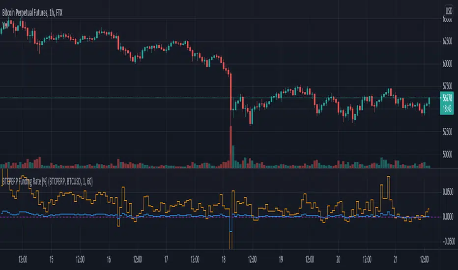
Funding Rate for FTX:BTCPERP (estimated) v0.1 Original credits goes to @Hayemaker, and @NeoButane for the TWAP portions of this script
By @davewhiiite, 2021-03-27
Version 0.1
Summary: The funding rate is the interest charged / credited to a perpetual futures trader for taking a long or short position. The direction of the funding rate is used as an indicator of trader sentiment (+ve = bullish; -ve = bearish), and therefore useful to plot in real time.
The FTX exchange has published the calculation of their funding rate as follows:
TWAP((future - index) / index) / 24
The formula here is the same, but expresses it in the more common % per 8hr duration:
funding = TWAP((future / index) - 1) * (8 / 24) * 100
For reference: future refers to the FTX bitcoin futures contract price (FTX:BTCPERP) and index is the spot price of bitcoin on the exchange (FTX:BTCUSD)
Additional notes:
Probably best to add to the indicator to a new pane, or as secondary axis
Plot this in combination with FTX:BTCPERP or FTX:BTCUSD, or chart of your choice to complement your bitcoin dashboard
Compare to funding rates published on ViewBase
questions? Ask me!
Universal Global SessionUniversal Global Session
This Script combines the world sessions of: Stocks, Forex, Bitcoin Kill Zones, strategic points, all configurable, in a single Script, to capitalize the opening and closing times of global exchanges as investment assets, becoming an Universal Global Session .
It is based on the great work of @oscarvs ( BITCOIN KILL ZONES v2 ) and the scripts of @ChrisMoody. Thank you Oscar and Chris for your excellent judgment and great work.
At the end of this writing you can find all the internet references of the extensive documentation that I present here. To maximize your benefits in the use of this Script, I recommend that you read the entire document to create an objective and practical criterion.
All the hours of the different exchanges are presented at GMT -6. In Market24hClock you can adjust it to your preferences.
After a deep investigation I have been able to show that the different world sessions reveal underlying investment cycles, where it is possible to find sustained changes in the nominal behavior of the trend before the passage from one session to another and in the natural overlaps between the sessions. These underlying movements generally occur 15 minutes before the start, close or overlap of the session, when the session properly starts and also 15 minutes after respectively. Therefore, this script is designed to highlight these particular trending behaviors. Try it, discover your own conclusions and let me know in the notes, thank you.
Foreign Exchange Market Hours
It is the schedule by which currency market participants can buy, sell, trade and speculate on currencies all over the world. It is open 24 hours a day during working days and closes on weekends, thanks to the fact that operations are carried out through a network of information systems, instead of physical exchanges that close at a certain time. It opens Monday morning at 8 am local time in Sydney —Australia— (which is equivalent to Sunday night at 7 pm, in New York City —United States—, according to Eastern Standard Time), and It closes at 5pm local time in New York City (which is equivalent to 6am Saturday morning in Sydney).
The Forex market is decentralized and driven by local sessions, where the hours of Forex trading are based on the opening range of each active country, becoming an efficient transfer mechanism for all participants. Four territories in particular stand out: Sydney, Tokyo, London and New York, where the highest volume of operations occurs when the sessions in London and New York overlap. Furthermore, Europe is complemented by major financial centers such as Paris, Frankfurt and Zurich. Each day of forex trading begins with the opening of Australia, then Asia, followed by Europe, and finally North America. As markets in one region close, another opens - or has already opened - and continues to trade in the currency market. The seven most traded currencies in the world are: the US dollar, the euro, the Japanese yen, the British pound, the Australian dollar, the Canadian dollar, and the New Zealand dollar.
Currencies are needed around the world for international trade, this means that operations are not dominated by a single exchange market, but rather involve a global network of brokers from around the world, such as banks, commercial companies, central banks, companies investment management, hedge funds, as well as retail forex brokers and global investors. Because this market operates in multiple time zones, it can be accessed at any time except during the weekend, therefore, there is continuously at least one open market and there are some hours of overlap between the closing of the market of one region and the opening of another. The international scope of currency trading means that there are always traders around the world making and satisfying demands for a particular currency.
The market involves a global network of exchanges and brokers from around the world, although time zones overlap, the generally accepted time zone for each region is as follows:
Sydney 5pm to 2am EST (10pm to 7am UTC)
London 3am to 12 noon EST (8pm to 5pm UTC)
New York 8am to 5pm EST (1pm to 10pm UTC)
Tokyo 7pm to 4am EST (12am to 9am UTC)
Trading Session
A financial asset trading session refers to a period of time that coincides with the daytime trading hours for a given location, it is a business day in the local financial market. This may vary according to the asset class and the country, therefore operators must know the hours of trading sessions for the securities and derivatives in which they are interested in trading. If investors can understand market hours and set proper targets, they will have a much greater chance of making a profit within a workable schedule.
Kill Zones
Kill zones are highly liquid events. Many different market participants often come together and perform around these events. The activity itself can be event-driven (margin calls or option exercise-related activity), portfolio management-driven (asset allocation rebalancing orders and closing buy-in), or institutionally driven (larger players needing liquidity to complete the size) or a combination of any of the three. This intense cross-current of activity at a very specific point in time often occurs near significant technical levels and the established trends emerging from these events often persist until the next Death Zone approaches or enters.
Kill Zones are evolving with time and the course of world history. Since the end of World War II, New York has slowly invaded London's place as the world center for commercial banking. So much so that during the latter part of the 20th century, New York was considered the new center of the financial universe. With the end of the cold war, that leadership appears to have shifted towards Europe and away from the United States. Furthermore, Japan has slowly lost its former dominance in the global economic landscape, while Beijing's has increased dramatically. Only time will tell how these death zones will evolve given the ever-changing political, economic, and socioeconomic influences of each region.
Financial Markets
New York
New York (NYSE Chicago, NASDAQ)
7:30 am - 2:00 pm
It is the second largest currency platform in the world, followed largely by foreign investors as it participates in 90% of all operations, where movements on the New York Stock Exchange (NYSE) can have an immediate effect (powerful) on the dollar, for example, when companies merge and acquisitions are finalized, the dollar can instantly gain or lose value.
A. Complementary Stock Exchanges
Brazil (BOVESPA - Brazilian Stock Exchange)
07:00 am - 02:55 pm
Canada (TSX - Toronto Stock Exchange)
07:30 am - 02:00 pm
New York (NYSE - New York Stock Exchange)
08:30 am - 03:00 pm
B. North American Trading Session
07:00 am - 03:00 pm
(from the beginning of the business day on NYSE and NASDAQ, until the end of the New York session)
New York, Chicago and Toronto (Canada) open the North American session. Characterized by the most aggressive trading within the markets, currency pairs show high volatility. As the US markets open, trading is still active in Europe, however trading volume generally decreases with the end of the European session and the overlap between the US and Europe.
C. Strategic Points
US main session starts in 1 hour
07:30 am
The euro tends to drop before the US session. The NYSE, CHX and TSX (Canada) trading sessions begin 1 hour after this strategic point. The North American session begins trading Forex at 07:00 am.
This constitutes the beginning of the overlap of the United States and the European market that spans from 07:00 am to 10:35 am, often called the best time to trade EUR / USD, it is the period of greatest liquidity for the main European currencies since it is where they have their widest daily ranges.
When New York opens at 07:00 am the most intense trading begins in both the US and European markets. The overlap of European and American trading sessions has 80% of the total average trading range for all currency pairs during US business hours and 70% of the total average trading range for all currency pairs during European business hours. The intersection of the US and European sessions are the most volatile overlapping hours of all.
Influential news and data for the USD are released between 07:30 am and 09:00 am and play the biggest role in the North American Session. These are the strategically most important moments of this activity period: 07:00 am, 08:00 am and 08:30 am.
The main session of operations in the United States and Canada begins
08:30 am
Start of main trading sessions in New York, Chicago and Toronto. The European session still overlaps the North American session and this is the time for large-scale unpredictable trading. The United States leads the market. It is difficult to interpret the news due to speculation. Trends develop very quickly and it is difficult to identify them, however trends (especially for the euro), which have developed during the overlap, often turn the other way when Europe exits the market.
Second hour of the US session and last hour of the European session
09:30 am
End of the European session
10:35 am
The trend of the euro will change rapidly after the end of the European session.
Last hour of the United States session
02:00 pm
Institutional clients and very large funds are very active during the first and last working hours of almost all stock exchanges, knowing this allows to better predict price movements in the opening and closing of large markets. Within the last trading hours of the secondary market session, a pullback can often be seen in the EUR / USD that continues until the opening of the Tokyo session. Generally it happens if there was an upward price movement before 04:00 pm - 05:00 pm.
End of the trade session in the United States
03:00 pm
D. Kill Zones
11:30 am - 1:30 pm
New York Kill Zone. The United States is still the world's largest economy, so by default, the New York opening carries a lot of weight and often comes with a huge injection of liquidity. In fact, most of the world's marketable assets are priced in US dollars, making political and economic activity within this region even more important. Because it is relatively late in the world's trading day, this Death Zone often sees violent price swings within its first hour, leading to the proven adage "never trust the first hour of trading in America. North.
---------------
London
London (LSE - London Stock Exchange)
02:00 am - 10:35 am
Britain dominates the currency markets around the world, and London is its main component. London, a central trading capital of the world, accounts for about 43% of world trade, many Forex trends often originate from London.
A. Complementary Stock Exchange
Dubai (DFM - Dubai Financial Market)
12:00 am - 03:50 am
Moscow (MOEX - Moscow Exchange)
12:30 am - 10:00 am
Germany (FWB - Frankfurt Stock Exchange)
01:00 am - 10:30 am
Afríca (JSE - Johannesburg Stock Exchange)
01:00 am - 09:00 am
Saudi Arabia (TADAWUL - Saudi Stock Exchange)
01:00 am - 06:00 am
Switzerland (SIX - Swiss Stock Exchange)
02:00 am - 10:30 am
B. European Trading Session
02:00 am - 11:00 am
(from the opening of the Frankfurt session to the close of the Order Book on the London Stock Exchange / Euronext)
It is a very liquid trading session, where trends are set that start during the first trading hours in Europe and generally continue until the beginning of the US session.
C. Middle East Trading Session
12:00 am - 06:00 am
(from the opening of the Dubai session to the end of the Riyadh session)
D. Strategic Points
European session begins
02:00 am
London, Frankfurt and Zurich Stock Exchange enter the market, overlap between Europe and Asia begins.
End of the Singapore and Asia sessions
03:00 am
The euro rises almost immediately or an hour after Singapore exits the market.
Middle East Oil Markets Completion Process
05:00 am
Operations are ending in the European-Asian market, at which time Dubai, Qatar and in another hour in Riyadh, which constitute the Middle East oil markets, are closing. Because oil trading is done in US dollars, and the region with the trading day coming to an end no longer needs the dollar, consequently, the euro tends to grow more frequently.
End of the Middle East trading session
06:00 am
E. Kill Zones
5:00 am - 7:00 am
London Kill Zone. Considered the center of the financial universe for more than 500 years, Europe still has a lot of influence in the banking world. Many older players use the European session to establish their positions. As such, the London Open often sees the most significant trend-setting activity on any trading day. In fact, it has been suggested that 80% of all weekly trends are set through the London Kill Zone on Tuesday.
F. Kill Zones (close)
2:00 pm - 4:00 pm
London Kill Zone (close).
---------------
Tokyo
Tokyo (JPX - Tokyo Stock Exchange)
06:00 pm - 12:00 am
It is the first Asian market to open, receiving most of the Asian trade, just ahead of Hong Kong and Singapore.
A. Complementary Stock Exchange
Singapore (SGX - Singapore Exchange)
07:00 pm - 03:00 am
Hong Kong (HKEx - Hong Kong Stock Exchange)
07:30 pm - 02:00 am
Shanghai (SSE - Shanghai Stock Exchange)
07:30 pm - 01:00 am
India (NSE - India National Stock Exchange)
09:45 pm - 04:00 am
B. Asian Trading Session
06:00 pm - 03:00 am
From the opening of the Tokyo session to the end of the Singapore session
The first major Asian market to open is Tokyo which has the largest market share and is the third largest Forex trading center in the world. Singapore opens in an hour, and then the Chinese markets: Shanghai and Hong Kong open 30 minutes later. With them, the trading volume increases and begins a large-scale operation in the Asia-Pacific region, offering more liquidity for the Asian-Pacific currencies and their crosses. When European countries open their doors, more liquidity will be offered to Asian and European crossings.
C. Strategic Points
Second hour of the Tokyo session
07:00 pm
This session also opens the Singapore market. The commercial dynamics grows in anticipation of the opening of the two largest Chinese markets in 30 minutes: Shanghai and Hong Kong, within these 30 minutes or just before the China session begins, the euro usually falls until the same moment of the opening of Shanghai and Hong Kong.
Second hour of the China session
08:30 pm
Hong Kong and Shanghai start trading and the euro usually grows for more than an hour. The EUR / USD pair mixes up as Asian exporters convert part of their earnings into both US dollars and euros.
Last hour of the Tokyo session
11:00 pm
End of the Tokyo session
12:00 am
If the euro has been actively declining up to this time, China will raise the euro after the Tokyo shutdown. Hong Kong, Shanghai and Singapore remain open and take matters into their own hands causing the growth of the euro. Asia is a huge commercial and industrial region with a large number of high-quality economic products and gigantic financial turnover, making the number of transactions on the stock exchanges huge during the Asian session. That is why traders, who entered the trade at the opening of the London session, should pay attention to their terminals when Asia exits the market.
End of the Shanghai session
01:00 am
The trade ends in Shanghai. This is the last trading hour of the Hong Kong session, during which market activity peaks.
D. Kill Zones
10:00 pm - 2:00 am
Asian Kill Zone. Considered the "Institutional" Zone, this zone represents both the launch pad for new trends as well as a recharge area for the post-American session. It is the beginning of a new day (or week) for the world and as such it makes sense that this zone often sets the tone for the remainder of the global business day. It is ideal to pay attention to the opening of Tokyo, Beijing and Sydney.
--------------
Sidney
Sydney (ASX - Australia Stock Exchange)
06:00 pm - 12:00 am
A. Complementary Stock Exchange
New Zealand (NZX - New Zealand Stock Exchange)
04:00 pm - 10:45 pm
It's where the global trading day officially begins. While it is the smallest of the megamarkets, it sees a lot of initial action when markets reopen Sunday afternoon as individual traders and financial institutions are trying to regroup after the long hiatus since Friday afternoon. On weekdays it constitutes the end of the current trading day where the change in the settlement date occurs.
B. Pacific Trading Session
04:00 pm - 12:00 am
(from the opening of the Wellington session to the end of the Sydney session)
Forex begins its business hours when Wellington (New Zealand Exchange) opens local time on Monday. Sydney (Australian Stock Exchange) opens in 2 hours. It is a session with a fairly low volatility, configuring itself as the calmest session of all. Strong movements appear when influential news is published and when the Pacific session overlaps the Asian Session.
C. Strategic Points
End of the Sydney session
12:00 am
---------------
Conclusions
The best time to trade is during overlaps in trading times between open markets. Overlaps equate to higher price ranges, creating greater opportunities.
Regarding press releases (news), it should be noted that these in the currency markets have the power to improve a normally slow trading period. When a major announcement is made regarding economic data, especially when it goes against the predicted forecast, the coin can lose or gain value in a matter of seconds. In general, the more economic growth a country produces, the more positive the economy is for international investors. Investment capital tends to flow to countries that are believed to have good growth prospects and subsequently good investment opportunities, leading to the strengthening of the country's exchange rate. Also, a country that has higher interest rates through its government bonds tends to attract investment capital as foreign investors seek high-yield opportunities. However, stable economic growth and attractive yields or interest rates are inextricably intertwined. It's important to take advantage of market overlaps and keep an eye out for press releases when setting up a trading schedule.
References:
www.investopedia.com
www.investopedia.com
www.investopedia.com
www.investopedia.com
market24hclock.com
market24hclock.com
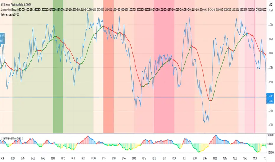
Square Root Moving AverageAbstract
This script computes moving averages which the weighting of the recent quarter takes up about a half weight.
This script also provides their upper bands and lower bands.
You can apply moving average or band strategies with this script.
Introduction
Moving average is a popular indicator which can eliminate market noise and observe trend.
There are several moving average related strategies used by many traders.
The first one is trade when the price is far from moving average.
To measure if the price is far from moving average, traders may need a lower band and an upper band.
Bollinger bands use standard derivation and Keltner channels use average true range.
In up trend, moving average and lower band can be support.
In ranging market, lower band can be support and upper band can be resistance.
In down trend, moving average and upper band can be resistance.
An another group of moving average strategy is comparing short term moving average and long term moving average.
Moving average cross, Awesome oscillators and MACD belong to this group.
The period and weightings of moving averages are also topics.
Period, as known as length, means how many days are computed by moving averages.
Weighting means how much weight the price of a day takes up in moving averages.
For simple moving averages, the weightings of each day are equal.
For most of non-simple moving averages, the weightings of more recent days are higher than the weightings of less recent days.
Many trading courses say the concept of trading strategies is more important than the settings of moving averages.
However, we can observe some characteristics of price movement to design the weightings of moving averages and make them more meaningful.
In this research, we use the observation that when there are no significant events, when the time frame becomes 4 times, the average true range becomes about 2 times.
For example, the average true range in 4-hour chart is about 2 times of the average true range in 1-hour chart; the average true range in 1-hour chart is about 2 times of the average true range in 15-minute chart.
Therefore, the goal of design is making the weighting of the most recent quarter is close to the weighting of the rest recent three quarters.
For example, for the 24-day moving average, the weighting of the most recent 6 days is close to the weighting of the rest 18 days.
Computing the weighting
The formula of moving average is
sum ( price of day n * weighting of day n ) / sum ( weighting of day n )
Day 1 is the most recent day and day k+1 is the day before day k.
For more convenient explanation, we don't expect sum ( weighting of day n ) is equal to 1.
To make the weighting of the most recent quarter is close to the weighting of the rest recent three quarters, we have
sum ( weighting of day 4n ) = 2 * sum ( weighting of day n )
If when weighting of day 1 is 1, we have
sum ( weighting of day n ) = sqrt ( n )
weighting of day n = sqrt ( n ) - sqrt ( n-1 )
weighting of day 2 ≒ 1.414 - 1.000 = 0.414
weighting of day 3 ≒ 1.732 - 1.414 = 0.318
weighting of day 4 ≒ 2.000 - 1.732 = 0.268
If we follow this formula, the weighting of day 1 is too strong and the moving average may be not stable.
To reduce the weighting of day 1 and keep the spirit of the formula, we can add a parameter (we call it as x_1w2b).
The formula becomes
weighting of day n = sqrt ( n+x_1w2b ) - sqrt ( n-1+x_1w2b )
if x_1w2b is 0.25, then we have
weighting of day 1 = sqrt(1.25) - sqrt(0.25) ≒ 1.1 - 0.5 = 0.6
weighting of day 2 = sqrt(2.25) - sqrt(1.25) ≒ 1.5 - 1.1 = 0.4
weighting of day 3 = sqrt(3.25) - sqrt(2.25) ≒ 1.8 - 1.5 = 0.3
weighting of day 4 = sqrt(4.25) - sqrt(3.25) ≒ 2.06 - 1.8 = 0.26
weighting of day 5 = sqrt(5.25) - sqrt(4.25) ≒ 2.3 - 2.06 = 0.24
weighting of day 6 = sqrt(6.25) - sqrt(5.25) ≒ 2.5 - 2.3 = 0.2
weighting of day 7 = sqrt(7.25) - sqrt(6.25) ≒ 2.7 - 2.5 = 0.2
What you see and can adjust in this script
This script plots three moving averages described above.
The short term one is default magenta, 6 days and 1 atr.
The middle term one is default yellow, 24 days and 2 atr.
The long term one is default green, 96 days and 4 atr.
I arrange the short term 6 days to make it close to sma(5).
The other twos are arranged according to 4x length and 2x atr.
There are 9 curves plotted by this script. I made the lower bands and the upper bands less clear than moving averages so it is less possible misrecognizing lower or upper bands as moving averages.
x_src : how to compute the reference price of a day, using 1 to 4 of open, high, low and close.
len : how many days are computed by moving averages
atr : how many days are computed by average true range
multi : the distance from the moving average to the lower band and the distance from the moving average to the lower band are equal to multi * average true range.
x_1w2b : adjust this number to avoid the weighting of day 1 from being too strong.
Conclusion
There are moving averages which the weighting of the most recent quarter is close to the weighting of the rest recent three quarters.
We can apply strategies based on moving averages. Like most of indicators, oversold does not always means it is an opportunity to buy.
If the short term lower band is close to the middle term moving average or the middle term lower band is close to the long term moving average, it may be potential support value.
References
Computing FIR Filters Using Arrays
How to trade with moving averages : the eight trading signals concluded by Granville
How to trade with Bollinger bands
How to trade with double Bollinger bands
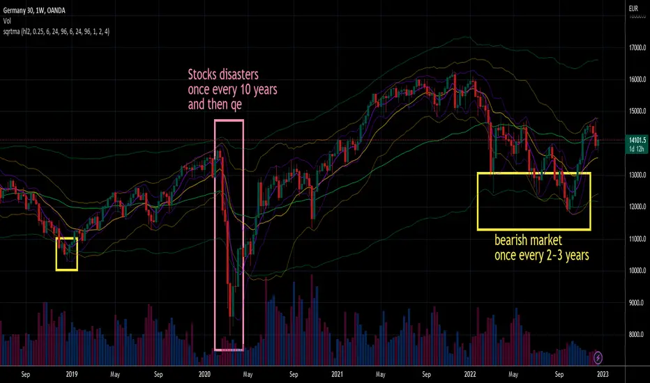
The Lazy Trader - Index (ETF) Trend Following Robot50/150 moving average, index (ETF) trend following robot. Coded for people who cannot psychologically handle dollar-cost-averaging through bear markets and extreme drawdowns (although DCA can produce better results eventually), this robot helps you to avoid bear markets. Be a fair-weathered friend of Mr Market, and only take up his offer when the sun is shining! Designed for the lazy trader who really doesn't care...
Recommended Chart Settings:
Asset Class: ETF
Time Frame: Daily
Necessary ETF Macro Conditions:
a) Country must have healthy demographics, good ratio of young > old
b) Country population must be increasing
c) Country must be experiencing price-inflation
Default Robot Settings:
Slow Moving Average: 50 (integer) //adjust to suit your underlying index
Fast Moving Average: 150 (integer) //adjust to suit your underlying index
Bullish Slope Angle: 5 (degrees) //up angle of moving averages
Bearish Slope Angle: -5 (degrees) //down angle of moving averages
Average True Range: 14 (integer) //input for slope-angle formula
Risk: 100 (%) //100% risk means using all equity per trade
ETF Test Results (Default Settings):
SPY (1993 to 2020, 27 years), 332% profit, 20 trades, 6.4 profit factor, 7% drawdown
EWG (1996 to 2020, 24 years), 310% profit, 18 trades, 3.7 profit factor, 10% drawdown
EWH (1996 to 2020, 24 years), 4% loss, 26 trades, 0.9 profit factor, 36% drawdown
QQQ (1999 to 2020, 21 years), 232% profit, 17 trades, 3.6 profit factor, 2% drawdown
EEM (2003 to 2020, 17 years), 73% profit, 17 trades, 1.1 profit factor, 3% drawdown
GXC (2007 to 2020, 13 years), 18% profit, 14 trades, 1.3 profit factor, 26% drawdown
BKF (2009 to 2020, 11 years), 11% profit, 13 trades, 1.2 profit factor, 33% drawdown
A longer time in the markets is better, with the exception of EWH. 6 out of 7 tested ETFs were profitable, feel free to test on your favourite ETF (default settings) and comment below.
Risk Warning:
Not tested on commodities nor other financial products like currencies (code will not work), feel free to leave comments below.
Moving Average Slope Angle Formula:
Reproduced and modified from source:

[fikira] Fibonacci MA / EMA's (Fibma / Fibema)I've made SMA/EMA's NOT based on the principle of the 2(1+1), 3(2+1),
5(3+2), 8(5+3), 13(8+5), 21(13+8), 34(21+13), 55(34+21), ... numbers,
but based on these following Fibonacci numbers:
0,236
0,382
0,500
0,618
0,764
1
Ending up with 2 series of Fibma / Fibema:
"Tiny Fibma / Fibema":
24, 38, 50, 62, 76, 100
"Big Fibma / Fibema":
236, 382, 500, 618, 764, 1000
IMHO it is striking how these lines often act as Resistance/Support,
although (except the 50, 100 & 500) they are not typical MA/EMA's.
They perform very well on every Timeframe as well!
Week:
3 Days:
1 Day:
4h:
1h:
Even on the 15 minutes:
Or 5':
Things to watch for:
Price compared to the Tiny or Big Fibma / Fibema (below or above)
Price compared to important Fibma / Fibema (for example below or
above MA 236, MA 764, MA 1000, ...)
Crossing of Fibma / Fibema 24/76, 236/764 and 38/62, 382/618
(bullish crossover = Lime coloured "cloud", bearish crossunder = Red coloured "cloud"),
...
I've made a change in barcolor if the close crosses the "Big Fibma / Fibema 500"
If price closes above MA/EMA 500, the first bar is yellow coloured,
if price stays above this level, candles are coloured lime/orange (= very bullish)
If price closes under MA/EMA 500, the first bar is purple,
if price stays under this level, candles are standard coloured (= very bearish)
Strategy will follow,
Thanks!
ATR - Baby WhaleScript that shows you the ATR and 0.5 ATR.
You can use this to define your stop loss level when you see a SFP.
Standard setting is the 24 period ATR. You can use this for a 1h chart (24 hours in a day).
So when you play on a 5m chart, you can change the setting to 12 period (12 5m candles in 1 hour).

Percentage Change Comparison [BVCC]This script allows you to input 2 different coins and plot % changes against each other.
Look Back is adjustable to account for different time frame windows. Default is 1, so each line will be graphed on a 1:1 ratio with the candle period selected on the chart. raising this number to 24 will plot the change across every 24 candles and so on. It's pretty interesting to move the input dialogue window out of the way and change this number, watching how the % gain comparisons change in real time.
Default coins to compare are set to BTCUSD and ETHUSD @ coinbase.

RSIVolume_2graf.01[wozdux] Tactics and strategy Tactics and strategy
The indicator combines 2 variants of the RSI indicator. The first option is calculated relative to the normal close price. The second option is calculated relative to the volume price. The volume price is calculated as the product of the volume price. For normal RSI, the default period is 9, for the volume price .
Settings. Level_close sets the width of the middle region, the oscillations of the indicator chart for the average of the closing price. Level_volume*close sets the critical level for the volume price. Period 24 (len1) specifies the RSI calculation period for the volume price. Period 9 (len3) specifies the RSI calculation period for the regular price.
The combination of two versions of the indicator helps to see more truthful information about the mood of buyers and sellers. When the volume price reaches its critical level of 8 units, it is a signal to a strong fall in the price. In this state, you should monitor the classic RSI. Thus, the classic RSI determines the tactical movement, and the volumetric RSI – strategic.
-------------------------------------
Тактика и стратегия
Индикатор совмещает в себе 2 варианта индикатора RSI. Первый вариант вычисляется относительно обычной цены закрытия. Второй вариант вычисляется относительно объемной цены. Объемную цену вычисляют как произведение цены на объем. Для обычного RSI по умолчанию берется период 9 , для объемной цены .
Настройки. Level_close задает ширину средней области колебания графика индикатора для обычной цены закрытия. Level_volume*close задает критический уровень для объемной цены. Период 24 (len1) задает период вычисления RSI для объемной цены. Период 9(len3) задает период вычисления RSI для обычной цены.
Сочетание двух вариантов индикатора помогает увидеть более правдивую информацию о настроениях покупателей и продавцов. Когда объемная цена достигает своего критического уровня 8 единиц, то это является сигналом к сильному падению цены. В этом состоянии следует следить за классической RSI. Таким образом классическое RSI определяет тактическое движение, а объемное RSI – стратегическое.