MarkovChainLibrary "MarkovChain"
Generic Markov Chain type functions.
---
A Markov chain or Markov process is a stochastic model describing a sequence of possible events in which the
probability of each event depends only on the state attained in the previous event.
---
reference:
Understanding Markov Chains, Examples and Applications. Second Edition. Book by Nicolas Privault.
en.wikipedia.org
www.geeksforgeeks.org
towardsdatascience.com
github.com
stats.stackexchange.com
timeseriesreasoning.com
www.ris-ai.com
github.com
gist.github.com
github.com
gist.github.com
writings.stephenwolfram.com
kevingal.com
towardsdatascience.com
spedygiorgio.github.io
github.com
www.projectrhea.org
method to_string(this)
Translate a Markov Chain object to a string format.
Namespace types: MC
Parameters:
this (MC) : `MC` . Markov Chain object.
Returns: string
method to_table(this, position, text_color, text_size)
Namespace types: MC
Parameters:
this (MC)
position (string)
text_color (color)
text_size (string)
method create_transition_matrix(this)
Namespace types: MC
Parameters:
this (MC)
method generate_transition_matrix(this)
Namespace types: MC
Parameters:
this (MC)
new_chain(states, name)
Parameters:
states (state )
name (string)
from_data(data, name)
Parameters:
data (string )
name (string)
method probability_at_step(this, target_step)
Namespace types: MC
Parameters:
this (MC)
target_step (int)
method state_at_step(this, start_state, target_state, target_step)
Namespace types: MC
Parameters:
this (MC)
start_state (int)
target_state (int)
target_step (int)
method forward(this, obs)
Namespace types: HMC
Parameters:
this (HMC)
obs (int )
method backward(this, obs)
Namespace types: HMC
Parameters:
this (HMC)
obs (int )
method viterbi(this, observations)
Namespace types: HMC
Parameters:
this (HMC)
observations (int )
method baumwelch(this, observations)
Namespace types: HMC
Parameters:
this (HMC)
observations (int )
Node
Target node.
Fields:
index (series int) : . Key index of the node.
probability (series float) : . Probability rate of activation.
state
State reference.
Fields:
name (series string) : . Name of the state.
index (series int) : . Key index of the state.
target_nodes (Node ) : . List of index references and probabilities to target states.
MC
Markov Chain reference object.
Fields:
name (series string) : . Name of the chain.
states (state ) : . List of state nodes and its name, index, targets and transition probabilities.
size (series int) : . Number of unique states
transitions (matrix) : . Transition matrix
HMC
Hidden Markov Chain reference object.
Fields:
name (series string) : . Name of thehidden chain.
states_hidden (state ) : . List of state nodes and its name, index, targets and transition probabilities.
states_obs (state ) : . List of state nodes and its name, index, targets and transition probabilities.
transitions (matrix) : . Transition matrix
emissions (matrix) : . Emission matrix
initial_distribution (float )
Sequence

FunctionProbabilityViterbiLibrary "FunctionProbabilityViterbi"
The Viterbi Algorithm calculates the most likely sequence of hidden states *(called Viterbi path)*
that results in a sequence of observed events.
viterbi(observations, transitions, emissions, initial_distribution)
Calculate most probable path in a Markov model.
Parameters:
observations (int ) : array . Observation states data.
transitions (matrix) : matrix . Transition probability table, (HxH, H:Hidden states).
emissions (matrix) : matrix . Emission probability table, (OxH, O:Observed states).
initial_distribution (float ) : array . Initial probability distribution for the hidden states.
Returns: array. Most probable path.

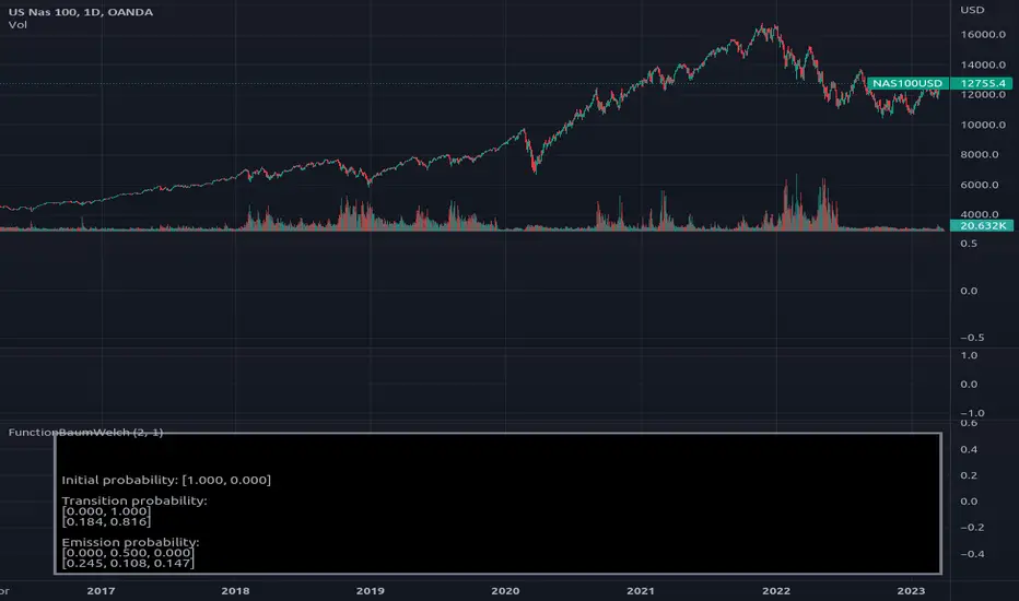
FunctionBaumWelchLibrary "FunctionBaumWelch"
Baum-Welch Algorithm, also known as Forward-Backward Algorithm, uses the well known EM algorithm
to find the maximum likelihood estimate of the parameters of a hidden Markov model given a set of observed
feature vectors.
---
### Function List:
> `forward (array pi, matrix a, matrix b, array obs)`
> `forward (array pi, matrix a, matrix b, array obs, bool scaling)`
> `backward (matrix a, matrix b, array obs)`
> `backward (matrix a, matrix b, array obs, array c)`
> `baumwelch (array observations, int nstates)`
> `baumwelch (array observations, array pi, matrix a, matrix b)`
---
### Reference:
> en.wikipedia.org
> github.com
> en.wikipedia.org
> www.rdocumentation.org
> www.rdocumentation.org
forward(pi, a, b, obs)
Computes forward probabilities for state `X` up to observation at time `k`, is defined as the
probability of observing sequence of observations `e_1 ... e_k` and that the state at time `k` is `X`.
Parameters:
pi (float ) : Initial probabilities.
a (matrix) : Transmissions, hidden transition matrix a or alpha = transition probability matrix of changing
states given a state matrix is size (M x M) where M is number of states.
b (matrix) : Emissions, matrix of observation probabilities b or beta = observation probabilities. Given
state matrix is size (M x O) where M is number of states and O is number of different
possible observations.
obs (int ) : List with actual state observation data.
Returns: - `matrix _alpha`: Forward probabilities. The probabilities are given on a logarithmic scale (natural logarithm). The first
dimension refers to the state and the second dimension to time.
forward(pi, a, b, obs, scaling)
Computes forward probabilities for state `X` up to observation at time `k`, is defined as the
probability of observing sequence of observations `e_1 ... e_k` and that the state at time `k` is `X`.
Parameters:
pi (float ) : Initial probabilities.
a (matrix) : Transmissions, hidden transition matrix a or alpha = transition probability matrix of changing
states given a state matrix is size (M x M) where M is number of states.
b (matrix) : Emissions, matrix of observation probabilities b or beta = observation probabilities. Given
state matrix is size (M x O) where M is number of states and O is number of different
possible observations.
obs (int ) : List with actual state observation data.
scaling (bool) : Normalize `alpha` scale.
Returns: - #### Tuple with:
> - `matrix _alpha`: Forward probabilities. The probabilities are given on a logarithmic scale (natural logarithm). The first
dimension refers to the state and the second dimension to time.
> - `array _c`: Array with normalization scale.
backward(a, b, obs)
Computes backward probabilities for state `X` and observation at time `k`, is defined as the probability of observing the sequence of observations `e_k+1, ... , e_n` under the condition that the state at time `k` is `X`.
Parameters:
a (matrix) : Transmissions, hidden transition matrix a or alpha = transition probability matrix of changing states
given a state matrix is size (M x M) where M is number of states
b (matrix) : Emissions, matrix of observation probabilities b or beta = observation probabilities. given state
matrix is size (M x O) where M is number of states and O is number of different possible observations
obs (int ) : Array with actual state observation data.
Returns: - `matrix _beta`: Backward probabilities. The probabilities are given on a logarithmic scale (natural logarithm). The first dimension refers to the state and the second dimension to time.
backward(a, b, obs, c)
Computes backward probabilities for state `X` and observation at time `k`, is defined as the probability of observing the sequence of observations `e_k+1, ... , e_n` under the condition that the state at time `k` is `X`.
Parameters:
a (matrix) : Transmissions, hidden transition matrix a or alpha = transition probability matrix of changing states
given a state matrix is size (M x M) where M is number of states
b (matrix) : Emissions, matrix of observation probabilities b or beta = observation probabilities. given state
matrix is size (M x O) where M is number of states and O is number of different possible observations
obs (int ) : Array with actual state observation data.
c (float ) : Array with Normalization scaling coefficients.
Returns: - `matrix _beta`: Backward probabilities. The probabilities are given on a logarithmic scale (natural logarithm). The first dimension refers to the state and the second dimension to time.
baumwelch(observations, nstates)
**(Random Initialization)** Baum–Welch algorithm is a special case of the expectation–maximization algorithm used to find the
unknown parameters of a hidden Markov model (HMM). It makes use of the forward-backward algorithm
to compute the statistics for the expectation step.
Parameters:
observations (int ) : List of observed states.
nstates (int)
Returns: - #### Tuple with:
> - `array _pi`: Initial probability distribution.
> - `matrix _a`: Transition probability matrix.
> - `matrix _b`: Emission probability matrix.
---
requires: `import RicardoSantos/WIPTensor/2 as Tensor`
baumwelch(observations, pi, a, b)
Baum–Welch algorithm is a special case of the expectation–maximization algorithm used to find the
unknown parameters of a hidden Markov model (HMM). It makes use of the forward-backward algorithm
to compute the statistics for the expectation step.
Parameters:
observations (int ) : List of observed states.
pi (float ) : Initial probaility distribution.
a (matrix) : Transmissions, hidden transition matrix a or alpha = transition probability matrix of changing states
given a state matrix is size (M x M) where M is number of states
b (matrix) : Emissions, matrix of observation probabilities b or beta = observation probabilities. given state
matrix is size (M x O) where M is number of states and O is number of different possible observations
Returns: - #### Tuple with:
> - `array _pi`: Initial probability distribution.
> - `matrix _a`: Transition probability matrix.
> - `matrix _b`: Emission probability matrix.
---
requires: `import RicardoSantos/WIPTensor/2 as Tensor`
FunctionDynamicTimeWarpingLibrary "FunctionDynamicTimeWarping"
"In time series analysis, dynamic time warping (DTW) is an algorithm for
measuring similarity between two temporal sequences, which may vary in
speed. For instance, similarities in walking could be detected using DTW,
even if one person was walking faster than the other, or if there were
accelerations and decelerations during the course of an observation.
DTW has been applied to temporal sequences of video, audio, and graphics
data — indeed, any data that can be turned into a linear sequence can be
analyzed with DTW. A well-known application has been automatic speech
recognition, to cope with different speaking speeds. Other applications
include speaker recognition and online signature recognition.
It can also be used in partial shape matching applications."
"Dynamic time warping is used in finance and econometrics to assess the
quality of the prediction versus real-world data."
~~ wikipedia
reference:
en.wikipedia.org
towardsdatascience.com
github.com
cost_matrix(a, b, w)
Dynamic Time Warping procedure.
Parameters:
a : array, data series.
b : array, data series.
w : int , minimum window size.
Returns: matrix optimum match matrix.
traceback(M)
perform a backtrace on the cost matrix and retrieve optimal paths and cost between arrays.
Parameters:
M : matrix, cost matrix.
Returns: tuple:
array aligned 1st array of indices.
array aligned 2nd array of indices.
float final cost.
reference:
github.com
report(a, b, w)
report ordered arrays, cost and cost matrix.
Parameters:
a : array, data series.
b : array, data series.
w : int , minimum window size.
Returns: string report.

ArrayGenerateLibrary "ArrayGenerate"
Functions to generate arrays.
sequence_int(start, end, step) returns a sequence of int numbers.
Parameters:
start : int, begining of sequence range.
end : int, end of sequence range.
step : int, step, default=1 .
Returns: int , array.
sequence_float(start, end, step) returns a sequence of float numbers.
Parameters:
start : float, begining of sequence range.
end : float, end of sequence range.
step : float, step, default=1.0 .
Returns: float , array.
sequence_from_series(src, length, shift, direction_forward) Creates a array from a series sample range.
Parameters:
src : series, any kind.
length : int, window period in bars to sample series.
shift : int, window period in bars to shift backwards the data sample, default=0.
direction_forward : bool, sample from start to end or end to start order, default=true.
Returns: float array
normal_distribution(size, mean, dev) Generate normal distribution random sample.
Parameters:
size : int, size of array
mean : float, mean of the sample, (default=0.0).
dev : float, deviation of the sample from the mean, (default=1.0).
Returns: float array.
log_spaced(length, start_exp, stop_exp) Generate a base 10 logarithmically spaced sample sequence.
Parameters:
length : int, length of the sequence.
start_exp : float, start exponent.
stop_exp : float, stop exponent.
Returns: float array.
linear_range(stop, start) Generate a linearly spaced sample vector within the inclusive interval (start, stop) and step 1.
Parameters:
stop : float, stop value.
start : float, start value, (default=0.0).
Returns: float array.
periodic_wave(length, sampling_rate, frequency, amplitude, phase, delay) Create a periodic wave.
Parameters:
length : int, the number of samples to generate.
sampling_rate : float, samples per time unit (Hz). Must be larger than twice the frequency to satisfy the Nyquist criterion.
frequency : float, frequency in periods per time unit (Hz).
amplitude : float, the length of the period when sampled at one sample per time unit. This is the interval of the periodic domain, a typical value is 1.0, or 2*Pi for angular functions.
phase : float, optional phase offset.
delay : int, optional delay, relative to the phase.
Returns: float array.
sinusoidal(length, sampling_rate, frequency, amplitude, mean, phase, delay) Create a Sine wave.
Parameters:
length : int, The number of samples to generate.
sampling_rate : float, Samples per time unit (Hz). Must be larger than twice the frequency to satisfy the Nyquist criterion.
frequency : float, Frequency in periods per time unit (Hz).
amplitude : float, The maximal reached peak.
mean : float, The mean, or DC part, of the signal.
phase : float, Optional phase offset.
delay : int, Optional delay, relative to the phase.
Returns: float array.
periodic_impulse(length, period, amplitude, delay) Create a periodic Kronecker Delta impulse sample array.
Parameters:
length : int, The number of samples to generate.
period : int, impulse sequence period.
amplitude : float, The maximal reached peak.
delay : int, Offset to the time axis. Zero or positive.
Returns: float array.