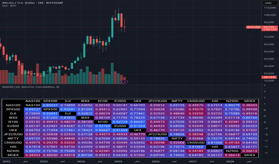
Multi Asset Similarity MatrixProvides a unique and visually stunning way to analyze the similarity between various stock market indices. This script uses a range of mathematical measures to calculate the correlation between different assets, such as indices, forex, crypto, etc..
Key Features:
Similarity Measures: The script offers a range of similarity measures to choose from, including SSD (Sum of Squared Differences), Euclidean Distance, Manhattan Distance, Minkowski Distance, Chebyshev Distance, Correlation Coefficient, Cosine Similarity, Camberra Index, Mean Absolute Error (MAE), Mean Squared Error (MSE), Lorentzian Function, Intersection, and Penrose Shape.
Asset Selection: Users can select the assets they want to analyze by entering a comma-separated list of tickers in the "Asset List" input field.
Color Gradient: The script uses a color gradient to represent the similarity values between each pair of indices, with red indicating low similarity and blue indicating high similarity.
How it Works:
The script calculates the source method (Returns or Volume Modified Returns) for each index using the sec function.
It then creates a matrix to hold the current values of each index over a specified window size (default is 10).
For each pair of indices, it applies the selected similarity measure using the select function and stores the result in a separate matrix.
The script calculates the maximum and minimum values of the similarity matrix to normalize the color gradient.
Finally, it creates a table with the index names as rows and columns, displaying the similarity values for each pair of indices using the calculated colors.
Visual Insights:
The indicator provides an intuitive way to visualize the relationships between different assets. By analyzing the color-coded tables, traders can gain insights into:
Which assets are highly correlated (blue) or uncorrelated (red)
The strength and direction of these correlations
Potential trading opportunities based on similarities and differences between assets
Overall, MASM is a powerful tool for market analysis and visualization, offering a unique perspective on the relationships between various assets.
~llama3
Similarity
Similar Price ActionDescription:
The indicator tries to find an area of N candles in history that has the most similar price action to the latest N candles. The maximum search distance is limited to 5000 candles. It works by calculating a coefficient for each candle and comparing it with the coefficient of the latest candle, thus searching for two closest values. The indicator highlights the latest N candles, as well as the most similar area found in the past, and also tries to predict future price based on the latest price and price directly after the most similar area that was found in the past.
Inputs:
- Length -> the area we are searching for is comprised of this many candles
- Lookback -> maximum distance in which a similar area can be found
- Function -> the function used to compare latest and past prices
Notes:
- The indicator is intended to work on smaller timeframes where the overall price difference is not very high, but can be used on any
SimilarityMeasuresLibrary "SimilarityMeasures"
Similarity measures are statistical methods used to quantify the distance between different data sets
or strings. There are various types of similarity measures, including those that compare:
- data points (SSD, Euclidean, Manhattan, Minkowski, Chebyshev, Correlation, Cosine, Camberra, MAE, MSE, Lorentzian, Intersection, Penrose Shape, Meehl),
- strings (Edit(Levenshtein), Lee, Hamming, Jaro),
- probability distributions (Mahalanobis, Fidelity, Bhattacharyya, Hellinger),
- sets (Kumar Hassebrook, Jaccard, Sorensen, Chi Square).
---
These measures are used in various fields such as data analysis, machine learning, and pattern recognition. They
help to compare and analyze similarities and differences between different data sets or strings, which
can be useful for making predictions, classifications, and decisions.
---
References:
en.wikipedia.org
cran.r-project.org
numerics.mathdotnet.com
github.com
github.com
github.com
Encyclopedia of Distances, doi.org
ssd(p, q)
Sum of squared difference for N dimensions.
Parameters:
p (float ) : `array` Vector with first numeric distribution.
q (float ) : `array` Vector with second numeric distribution.
Returns: Measure of distance that calculates the squared euclidean distance.
euclidean(p, q)
Euclidean distance for N dimensions.
Parameters:
p (float ) : `array` Vector with first numeric distribution.
q (float ) : `array` Vector with second numeric distribution.
Returns: Measure of distance that calculates the straight-line (or Euclidean).
manhattan(p, q)
Manhattan distance for N dimensions.
Parameters:
p (float ) : `array` Vector with first numeric distribution.
q (float ) : `array` Vector with second numeric distribution.
Returns: Measure of absolute differences between both points.
minkowski(p, q, p_value)
Minkowsky Distance for N dimensions.
Parameters:
p (float ) : `array` Vector with first numeric distribution.
q (float ) : `array` Vector with second numeric distribution.
p_value (float) : `float` P value, default=1.0(1: manhatan, 2: euclidean), does not support chebychev.
Returns: Measure of similarity in the normed vector space.
chebyshev(p, q)
Chebyshev distance for N dimensions.
Parameters:
p (float ) : `array` Vector with first numeric distribution.
q (float ) : `array` Vector with second numeric distribution.
Returns: Measure of maximum absolute difference.
correlation(p, q)
Correlation distance for N dimensions.
Parameters:
p (float ) : `array` Vector with first numeric distribution.
q (float ) : `array` Vector with second numeric distribution.
Returns: Measure of maximum absolute difference.
cosine(p, q)
Cosine distance between provided vectors.
Parameters:
p (float ) : `array` 1D Vector.
q (float ) : `array` 1D Vector.
Returns: The Cosine distance between vectors `p` and `q`.
---
angiogenesis.dkfz.de
camberra(p, q)
Camberra distance for N dimensions.
Parameters:
p (float ) : `array` Vector with first numeric distribution.
q (float ) : `array` Vector with second numeric distribution.
Returns: Weighted measure of absolute differences between both points.
mae(p, q)
Mean absolute error is a normalized version of the sum of absolute difference (manhattan).
Parameters:
p (float ) : `array` Vector with first numeric distribution.
q (float ) : `array` Vector with second numeric distribution.
Returns: Mean absolute error of vectors `p` and `q`.
mse(p, q)
Mean squared error is a normalized version of the sum of squared difference.
Parameters:
p (float ) : `array` Vector with first numeric distribution.
q (float ) : `array` Vector with second numeric distribution.
Returns: Mean squared error of vectors `p` and `q`.
lorentzian(p, q)
Lorentzian distance between provided vectors.
Parameters:
p (float ) : `array` Vector with first numeric distribution.
q (float ) : `array` Vector with second numeric distribution.
Returns: Lorentzian distance of vectors `p` and `q`.
---
angiogenesis.dkfz.de
intersection(p, q)
Intersection distance between provided vectors.
Parameters:
p (float ) : `array` Vector with first numeric distribution.
q (float ) : `array` Vector with second numeric distribution.
Returns: Intersection distance of vectors `p` and `q`.
---
angiogenesis.dkfz.de
penrose(p, q)
Penrose Shape distance between provided vectors.
Parameters:
p (float ) : `array` Vector with first numeric distribution.
q (float ) : `array` Vector with second numeric distribution.
Returns: Penrose shape distance of vectors `p` and `q`.
---
angiogenesis.dkfz.de
meehl(p, q)
Meehl distance between provided vectors.
Parameters:
p (float ) : `array` Vector with first numeric distribution.
q (float ) : `array` Vector with second numeric distribution.
Returns: Meehl distance of vectors `p` and `q`.
---
angiogenesis.dkfz.de
edit(x, y)
Edit (aka Levenshtein) distance for indexed strings.
Parameters:
x (int ) : `array` Indexed array.
y (int ) : `array` Indexed array.
Returns: Number of deletions, insertions, or substitutions required to transform source string into target string.
---
generated description:
The Edit distance is a measure of similarity used to compare two strings. It is defined as the minimum number of
operations (insertions, deletions, or substitutions) required to transform one string into another. The operations
are performed on the characters of the strings, and the cost of each operation depends on the specific algorithm
used.
The Edit distance is widely used in various applications such as spell checking, text similarity, and machine
translation. It can also be used for other purposes like finding the closest match between two strings or
identifying the common prefixes or suffixes between them.
---
github.com
www.red-gate.com
planetcalc.com
lee(x, y, dsize)
Distance between two indexed strings of equal length.
Parameters:
x (int ) : `array` Indexed array.
y (int ) : `array` Indexed array.
dsize (int) : `int` Dictionary size.
Returns: Distance between two strings by accounting for dictionary size.
---
www.johndcook.com
hamming(x, y)
Distance between two indexed strings of equal length.
Parameters:
x (int ) : `array` Indexed array.
y (int ) : `array` Indexed array.
Returns: Length of different components on both sequences.
---
en.wikipedia.org
jaro(x, y)
Distance between two indexed strings.
Parameters:
x (int ) : `array` Indexed array.
y (int ) : `array` Indexed array.
Returns: Measure of two strings' similarity: the higher the value, the more similar the strings are.
The score is normalized such that `0` equates to no similarities and `1` is an exact match.
---
rosettacode.org
mahalanobis(p, q, VI)
Mahalanobis distance between two vectors with population inverse covariance matrix.
Parameters:
p (float ) : `array` 1D Vector.
q (float ) : `array` 1D Vector.
VI (matrix) : `matrix` Inverse of the covariance matrix.
Returns: The mahalanobis distance between vectors `p` and `q`.
---
people.revoledu.com
stat.ethz.ch
docs.scipy.org
fidelity(p, q)
Fidelity distance between provided vectors.
Parameters:
p (float ) : `array` 1D Vector.
q (float ) : `array` 1D Vector.
Returns: The Bhattacharyya Coefficient between vectors `p` and `q`.
---
en.wikipedia.org
bhattacharyya(p, q)
Bhattacharyya distance between provided vectors.
Parameters:
p (float ) : `array` 1D Vector.
q (float ) : `array` 1D Vector.
Returns: The Bhattacharyya distance between vectors `p` and `q`.
---
en.wikipedia.org
hellinger(p, q)
Hellinger distance between provided vectors.
Parameters:
p (float ) : `array` 1D Vector.
q (float ) : `array` 1D Vector.
Returns: The hellinger distance between vectors `p` and `q`.
---
en.wikipedia.org
jamesmccaffrey.wordpress.com
kumar_hassebrook(p, q)
Kumar Hassebrook distance between provided vectors.
Parameters:
p (float ) : `array` 1D Vector.
q (float ) : `array` 1D Vector.
Returns: The Kumar Hassebrook distance between vectors `p` and `q`.
---
github.com
jaccard(p, q)
Jaccard distance between provided vectors.
Parameters:
p (float ) : `array` 1D Vector.
q (float ) : `array` 1D Vector.
Returns: The Jaccard distance between vectors `p` and `q`.
---
github.com
sorensen(p, q)
Sorensen distance between provided vectors.
Parameters:
p (float ) : `array` 1D Vector.
q (float ) : `array` 1D Vector.
Returns: The Sorensen distance between vectors `p` and `q`.
---
people.revoledu.com
chi_square(p, q, eps)
Chi Square distance between provided vectors.
Parameters:
p (float ) : `array` 1D Vector.
q (float ) : `array` 1D Vector.
eps (float)
Returns: The Chi Square distance between vectors `p` and `q`.
---
uw.pressbooks.pub
stats.stackexchange.com
www.itl.nist.gov
kulczynsky(p, q, eps)
Kulczynsky distance between provided vectors.
Parameters:
p (float ) : `array` 1D Vector.
q (float ) : `array` 1D Vector.
eps (float)
Returns: The Kulczynsky distance between vectors `p` and `q`.
---
github.com
FunctionCosineSimilarityLibrary "FunctionCosineSimilarity"
Cosine Similarity method.
function(sample_a, sample_b) Measure the similarity of 2 vectors.
Parameters:
sample_a : float array, values.
sample_b : float array, values.
Returns: float.
diss(cosim) Dissimilarity helper function.
Parameters:
cosim : float, cosine similarity value (0 > 1)
Returns: float
The Echo Forecast [LuxAlgo]This indicator uses a simple time series forecasting method derived from the similarity between recent prices and similar/dissimilar historical prices. We named this method "ECHO".
This method originally assumes that future prices can be estimated from a historical series of observations that are most similar to the most recent price variations. This similarity is quantified using the correlation coefficient. Such an assumption can prove to be relatively effective with the forecasting of a periodic time series. We later introduced the ability to select dissimilar series of observations for further experimentation.
This forecasting technique is closely inspired by the analogue method introduced by Lorenz for the prediction of atmospheric data.
1. Settings
Evaluation Window: Window size used for finding historical observations similar/dissimilar to recent observations. The total evaluation window is equal to "Forecast Window" + "Evaluation Window"
Forecast Window: Determines the forecasting horizon.
Forecast Mode: Determines whether to choose historical series similar or dissimilar to the recent price observations.
Forecast Construction: Determines how the forecast is constructed. See "Usage" below.
Src: Source input of the forecast
Other style settings are self-explanatory.
2. Usage
This tool can be used to forecast future trends but also to indicate which historical variations have the highest degree of similarity/dissimilarity between the observations in the orange zone.
The forecasting window determines the prices segment (in orange) to be used as a reference for the search of the most similar/dissimilar historical price segment (in green) within the gray area.
Most forecasting techniques highly benefit from a detrended series. Due to the nature of this method, we highly recommend applying it to a detrended and periodic series.
You can see above the method is applied on a smooth periodic oscillator and a momentum oscillator.
The construction of the forecast is made from the price changes obtained in the green area, denoted as w(t) . Using the "Cumulative" options we construct the forecast from the cumulative sum of w(t) . Finally, we add the most recent price value to this cumulated series.
Using the "Mean" options will add the series w(t) with the mean of the prices within the orange segment.
Finally the "Linreg" will add the series w(t) to an extrapolated linear regression fit to the prices within the orange segment.