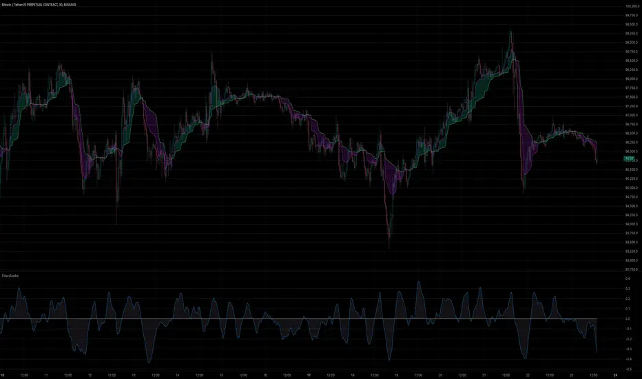
[GYTS] FiltersToolkit LibraryFiltersToolkit Library
🌸 Part of GoemonYae Trading System (GYTS) 🌸
🌸 --------- 1. INTRODUCTION --------- 🌸
💮 What Does This Library Contain?
This library is a curated collection of high-performance digital signal processing (DSP) filters and auxiliary functions designed specifically for financial time series analysis. It includes a shortlist of our favourite and best performing filters — each rigorously tested and selected for their responsiveness, minimal lag and robustness in diverse market conditions. These tools form an integral part of the GoemonYae Trading System (GYTS), chosen for their unique characteristics in handling market data.
The library contains two main categories:
1. Smoothing filters (low-pass filters and moving averages) for e.g. denoising, trend following
2. Detrending tools (high-pass and band-pass filters, known as "oscillators") for e.g. mean reversion
This collection is finely tuned for practical trading applications and is therefore not meant to be exhaustive. However, will continue to expand as we discover and validate new filtering techniques. I welcome collaboration and suggestions for novel approaches.
🌸 ——— 2. ADDED VALUE ——— 🌸
💮 Unified syntax and comprehensive documentation
The FiltersToolkit Library brings together a wide array of valuable filters under a unified, intuitive syntax. Each function is thoroughly documented, with clear explanations and academic sources that underline the mathematical rigour behind the methods. This level of documentation not only facilitates integration into trading strategies but also helps underlying the underlying concepts and rationale.
💮 Optimised performance and readability
The code prioritizes computational efficiency while maintaining readability. Key optimizations include:
- Minimizing redundant calculations in recursive filters
- Smart coefficient caching
- Efficient state management
- Vectorized operations where applicable
💮 Enhanced functionality and flexibility
Some filters in this library introduce extended functionality beyond the original publications. For instance, the MESA Adaptive Moving Average (MAMA) and Ehlers’ Combined Bandpass Filter incorporate multiple variations found in the literature, thereby providing traders with flexible tools that can be fine-tuned to different market conditions.
🌸 ——— 3. THE FILTERS ——— 🌸
💮 Hilbert Transform Function
This function implements the Hilbert Transform as utilised by John Ehlers. It converts a real-valued time series into its analytic signal, enabling the extraction of instantaneous phase and frequency information—an essential step in adaptive filtering.
Source: John Ehlers - "Rocket Science for Traders" (2001), "TASC 2001 V. 19:9", "Cybernetic Analysis for Stocks and Futures" (2004)
💮 Homodyne Discriminator
By leveraging the Hilbert Transform, this function computes the dominant cycle period through a Homodyne Discriminator. It extracts the in-phase and quadrature components of the signal, facilitating a robust estimation of the underlying cycle characteristics.
Source: John Ehlers - "Rocket Science for Traders" (2001), "TASC 2001 V. 19:9", "Cybernetic Analysis for Stocks and Futures" (2004)
💮 MESA Adaptive Moving Average (MAMA)
An advanced dual-stage adaptive moving average, this function outputs both the MAMA and its companion FAMA. It combines adaptive alpha computation with elements from Kaufman’s Adaptive Moving Average (KAMA) to provide a responsive and reliable trend indicator.
Source: John Ehlers - "Rocket Science for Traders" (2001), "TASC 2001 V. 19:9", "Cybernetic Analysis for Stocks and Futures" (2004)
💮 BiQuad Filters
A family of second-order recursive filters offering exceptional control over frequency response:
- High-pass filter for detrending
- Low-pass filter for smooth trend following
- Band-pass filter for cycle isolation
The quality factor (Q) parameter allows fine-tuning of the resonance characteristics, making these filters highly adaptable to different market conditions.
Source: Robert Bristow-Johnson's Audio EQ Cookbook, implemented by @The_Peaceful_Lizard
💮 Relative Vigor Index (RVI)
This filter evaluates the strength of a trend by comparing the closing price to the trading range. Operating similarly to a band-pass filter, the RVI provides insights into market momentum and potential reversals.
Source: John Ehlers – “Cybernetic Analysis for Stocks and Futures” (2004)
💮 Cyber Cycle
The Cyber Cycle filter emphasises market cycles by smoothing out noise and highlighting the dominant cyclical behaviour. It is particularly useful for detecting trend reversals and cyclical patterns in the price data.
Source: John Ehlers – “Cybernetic Analysis for Stocks and Futures” (2004)
💮 Butterworth High Pass Filter
Inspired by the classical Butterworth design, this filter achieves a maximally flat magnitude response in the passband while effectively removing low-frequency trends. Its design minimises phase distortion, which is vital for accurate signal interpretation.
Source: John Ehlers – “Cybernetic Analysis for Stocks and Futures” (2004)
💮 2-Pole SuperSmoother
Employing a two-pole design, the SuperSmoother filter reduces high-frequency noise with minimal lag. It is engineered to preserve trend integrity while offering a smooth output even in noisy market conditions.
Source: John Ehlers – “Cybernetic Analysis for Stocks and Futures” (2004)
💮 3-Pole SuperSmoother
An extension of the 2-pole design, the 3-pole SuperSmoother further attenuates high-frequency noise. Its additional pole delivers enhanced smoothing at the cost of slightly increased lag.
Source: John Ehlers – “Cybernetic Analysis for Stocks and Futures” (2004)
💮 Adaptive Directional Volatility Moving Average (ADXVma)
This adaptive moving average adjusts its smoothing factor based on directional volatility. By combining true range and directional movement measurements, it remains exceptionally flat during ranging markets and responsive during directional moves.
Source: Various implementations across platforms, unified and optimized
💮 Ehlers Combined Bandpass Filter with Automated Gain Control (AGC)
This sophisticated filter merges a highpass pre-processing stage with a bandpass filter. An integrated Automated Gain Control normalises the output to a consistent range, while offering both regular and truncated recursive formulations to manage lag.
Source: John F. Ehlers – “Truncated Indicators” (2020), “Cycle Analytics for Traders” (2013)
💮 Voss Predictive Filter
A forward-looking filter that predicts future values of a band-limited signal in real time. By utilising multiple time-delayed feedback terms, it provides anticipatory coupling and delivers a short-term predictive signal.
Source: John Ehlers - "A Peek Into The Future" (TASC 2019-08)
💮 Adaptive Autonomous Recursive Moving Average (A2RMA)
This filter dynamically adjusts its smoothing through an adaptive mechanism based on an efficiency ratio and a dynamic threshold. A double application of an adaptive moving average ensures both responsiveness and stability in volatile and ranging markets alike. Very flat response when properly tuned.
Source: @alexgrover (2019)
💮 Ultimate Smoother (2-Pole)
The Ultimate Smoother filter is engineered to achieve near-zero lag in its passband by subtracting a high-pass response from an all-pass response. This creates a filter that maintains signal fidelity at low frequencies while effectively filtering higher frequencies at the expense of slight overshooting.
Source: John Ehlers - TASC 2024-04 "The Ultimate Smoother"
Note: This library is actively maintained and enhanced. Suggestions for additional filters or improvements are welcome through the usual channels. The source code contains a list of tested filters that did not make it into the curated collection.
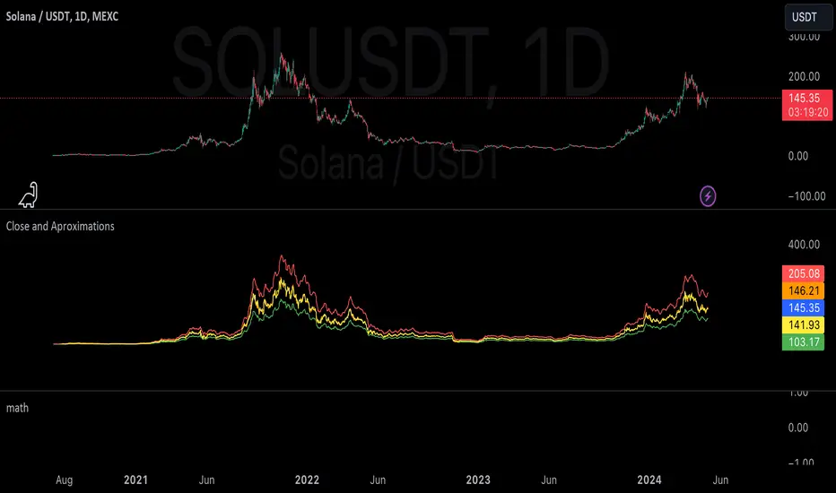
Smoothing
mathLibrary "math"
It's a library of discrete aproximations of a price or Series float it uses Fourier Discrete transform, Laplace Discrete Original and Modified transform and Euler's Theoreum for Homogenus White noice operations. Calling functions without source value it automatically take close as the default source value.
Here is a picture of Laplace and Fourier approximated close prices from this library:
Copy this indicator and try it yourself:
import AutomatedTradingAlgorithms/math/1 as math
//@version=5
indicator("Close Price with Aproximations", shorttitle="Close and Aproximations", overlay=false)
// Sample input data (replace this with your own data)
inputData = close
// Plot Close Price
plot(inputData, color=color.blue, title="Close Price")
ltf32_result = math.LTF32(a=0.01)
plot(ltf32_result, color=color.green, title="LTF32 Aproximation")
fft_result = math.FFT()
plot(fft_result, color=color.red, title="Fourier Aproximation")
wavelet_result = math.Wavelet()
plot(wavelet_result, color=color.orange, title="Wavelet Aproximation")
wavelet_std_result = math.Wavelet_std()
plot(wavelet_std_result, color=color.yellow, title="Wavelet_std Aproximation")
DFT3(xval, _dir)
Discrete Fourier Transform with last 3 points
Parameters:
xval (float) : Source series
_dir (int) : Direction parameter
Returns: Aproxiated source value
DFT2(xval, _dir)
Discrete Fourier Transform with last 2 points
Parameters:
xval (float) : Source series
_dir (int) : Direction parameter
Returns: Aproxiated source value
FFT(xval)
Fast Fourier Transform once. It aproximates usig last 3 points.
Parameters:
xval (float) : Source series
Returns: Aproxiated source value
DFT32(xval)
Combined Discrete Fourier Transforms of DFT3 and DTF2 it aproximates last point by first
aproximating last 3 ponts and than using last 2 points of the previus.
Parameters:
xval (float) : Source series
Returns: Aproxiated source value
DTF32(xval)
Combined Discrete Fourier Transforms of DFT3 and DTF2 it aproximates last point by first
aproximating last 3 ponts and than using last 2 points of the previus.
Parameters:
xval (float) : Source series
Returns: Aproxiated source value
LFT3(xval, _dir, a)
Discrete Laplace Transform with last 3 points
Parameters:
xval (float) : Source series
_dir (int) : Direction parameter
a (float) : laplace coeficient
Returns: Aproxiated source value
LFT2(xval, _dir, a)
Discrete Laplace Transform with last 2 points
Parameters:
xval (float) : Source series
_dir (int) : Direction parameter
a (float) : laplace coeficient
Returns: Aproxiated source value
LFT(xval, a)
Fast Laplace Transform once. It aproximates usig last 3 points.
Parameters:
xval (float) : Source series
a (float) : laplace coeficient
Returns: Aproxiated source value
LFT32(xval, a)
Combined Discrete Laplace Transforms of LFT3 and LTF2 it aproximates last point by first
aproximating last 3 ponts and than using last 2 points of the previus.
Parameters:
xval (float) : Source series
a (float) : laplace coeficient
Returns: Aproxiated source value
LTF32(xval, a)
Combined Discrete Laplace Transforms of LFT3 and LTF2 it aproximates last point by first
aproximating last 3 ponts and than using last 2 points of the previus.
Parameters:
xval (float) : Source series
a (float) : laplace coeficient
Returns: Aproxiated source value
whitenoise(indic_, _devided, minEmaLength, maxEmaLength, src)
Ehler's Universal Oscillator with White Noise, without extra aproximated src.
It uses dinamic EMA to aproximate indicator and thus reducing noise.
Parameters:
indic_ (float) : Input series for the indicator values to be smoothed
_devided (int) : Divisor for oscillator calculations
minEmaLength (int) : Minimum EMA length
maxEmaLength (int) : Maximum EMA length
src (float) : Source series
Returns: Smoothed indicator value
whitenoise(indic_, dft1, _devided, minEmaLength, maxEmaLength, src)
Ehler's Universal Oscillator with White Noise and DFT1.
It uses src and sproxiated src (dft1) to clearly define white noice.
It uses dinamic EMA to aproximate indicator and thus reducing noise.
Parameters:
indic_ (float) : Input series for the indicator values to be smoothed
dft1 (float) : Aproximated src value for white noice calculation
_devided (int) : Divisor for oscillator calculations
minEmaLength (int) : Minimum EMA length
maxEmaLength (int) : Maximum EMA length
src (float) : Source series
Returns: Smoothed indicator value
smooth(dft1, indic__, _devided, minEmaLength, maxEmaLength, src)
Smoothing source value with help of indicator series and aproximated source value
It uses src and sproxiated src (dft1) to clearly define white noice.
It uses dinamic EMA to aproximate src and thus reducing noise.
Parameters:
dft1 (float) : Value to be smoothed.
indic__ (float) : Optional input for indicator to help smooth dft1 (default is FFT)
_devided (int) : Divisor for smoothing calculations
minEmaLength (int) : Minimum EMA length
maxEmaLength (int) : Maximum EMA length
src (float) : Source series
Returns: Smoothed source (src) series
smooth(indic__, _devided, minEmaLength, maxEmaLength, src)
Smoothing source value with help of indicator series
It uses dinamic EMA to aproximate src and thus reducing noise.
Parameters:
indic__ (float) : Optional input for indicator to help smooth dft1 (default is FFT)
_devided (int) : Divisor for smoothing calculations
minEmaLength (int) : Minimum EMA length
maxEmaLength (int) : Maximum EMA length
src (float) : Source series
Returns: Smoothed src series
vzo_ema(src, len)
Volume Zone Oscillator with EMA smoothing
Parameters:
src (float) : Source series
len (simple int) : Length parameter for EMA
Returns: VZO value
vzo_sma(src, len)
Volume Zone Oscillator with SMA smoothing
Parameters:
src (float) : Source series
len (int) : Length parameter for SMA
Returns: VZO value
vzo_wma(src, len)
Volume Zone Oscillator with WMA smoothing
Parameters:
src (float) : Source series
len (int) : Length parameter for WMA
Returns: VZO value
alma2(series, windowsize, offset, sigma)
Arnaud Legoux Moving Average 2 accepts sigma as series float
Parameters:
series (float) : Input series
windowsize (int) : Size of the moving average window
offset (float) : Offset parameter
sigma (float) : Sigma parameter
Returns: ALMA value
Wavelet(src, len, offset, sigma)
Aproxiates srt using Discrete wavelet transform.
Parameters:
src (float) : Source series
len (int) : Length parameter for ALMA
offset (simple float)
sigma (simple float)
Returns: Wavelet-transformed series
Wavelet_std(src, len, offset, mag)
Aproxiates srt using Discrete wavelet transform with standard deviation as a magnitude.
Parameters:
src (float) : Source series
len (int) : Length parameter for ALMA
offset (float) : Offset parameter for ALMA
mag (int) : Magnitude parameter for standard deviation
Returns: Wavelet-transformed series
LaplaceTransform(xval, N, a)
Original Laplace Transform over N set of close prices
Parameters:
xval (float) : series to aproximate
N (int) : number of close prices in calculations
a (float) : laplace coeficient
Returns: Aproxiated source value
NLaplaceTransform(xval, N, a, repeat)
Y repetirions on Original Laplace Transform over N set of close prices, each time N-k set of close prices
Parameters:
xval (float) : series to aproximate
N (int) : number of close prices in calculations
a (float) : laplace coeficient
repeat (int) : number of repetitions
Returns: Aproxiated source value
LaplaceTransformsum(xval, N, a, b)
Sum of 2 exponent coeficient of Laplace Transform over N set of close prices
Parameters:
xval (float) : series to aproximate
N (int) : number of close prices in calculations
a (float) : laplace coeficient
b (float) : second laplace coeficient
Returns: Aproxiated source value
NLaplaceTransformdiff(xval, N, a, b, repeat)
Difference of 2 exponent coeficient of Laplace Transform over N set of close prices
Parameters:
xval (float) : series to aproximate
N (int) : number of close prices in calculations
a (float) : laplace coeficient
b (float) : second laplace coeficient
repeat (int) : number of repetitions
Returns: Aproxiated source value
N_divLaplaceTransformdiff(xval, N, a, b, repeat)
N repetitions of Difference of 2 exponent coeficient of Laplace Transform over N set of close prices, with dynamic rotation
Parameters:
xval (float) : series to aproximate
N (int) : number of close prices in calculations
a (float) : laplace coeficient
b (float) : second laplace coeficient
repeat (int) : number of repetitions
Returns: Aproxiated source value
LaplaceTransformdiff(xval, N, a, b)
Difference of 2 exponent coeficient of Laplace Transform over N set of close prices
Parameters:
xval (float) : series to aproximate
N (int) : number of close prices in calculations
a (float) : laplace coeficient
b (float) : second laplace coeficient
Returns: Aproxiated source value
NLaplaceTransformdiffFrom2(xval, N, a, b, repeat)
N repetitions of Difference of 2 exponent coeficient of Laplace Transform over N set of close prices, second element has for 1 higher exponent factor
Parameters:
xval (float) : series to aproximate
N (int) : number of close prices in calculations
a (float) : laplace coeficient
b (float) : second laplace coeficient
repeat (int) : number of repetitions
Returns: Aproxiated source value
N_divLaplaceTransformdiffFrom2(xval, N, a, b, repeat)
N repetitions of Difference of 2 exponent coeficient of Laplace Transform over N set of close prices, second element has for 1 higher exponent factor, dynamic rotation
Parameters:
xval (float) : series to aproximate
N (int) : number of close prices in calculations
a (float) : laplace coeficient
b (float) : second laplace coeficient
repeat (int) : number of repetitions
Returns: Aproxiated source value
LaplaceTransformdiffFrom2(xval, N, a, b)
Difference of 2 exponent coeficient of Laplace Transform over N set of close prices, second element has for 1 higher exponent factor
Parameters:
xval (float) : series to aproximate
N (int) : number of close prices in calculations
a (float) : laplace coeficient
b (float) : second laplace coeficient
Returns: Aproxiated source value
Library_SmoothersLibrary "Library_Smoothers"
CorrectedMA(Src, Len)
CorrectedMA The strengths of the corrected Average (CA) is that the current value of the time series must exceed a the current volatility-dependent threshold, so that the filter increases or falls, avoiding false signals when the trend is in a weak phase.
Parameters:
Src
Len
Returns: The Corrected source.
EHMA(src, len)
EMA Exponential Moving Average.
Parameters:
src : Source to act upon
len
Returns: EMA of source
FRAMA(src, len, FC, SC)
FRAMA Fractal Adaptive Moving Average
Parameters:
src : Source to act upon
len : Length of moving average
FC : Fast moving average
SC : Slow moving average
Returns: FRAMA of source
Jurik(src, length, phase, power)
Jurik A low lag filter
Parameters:
src : Source
length : Length for smoothing
phase : Phase range is ±100
power : Mathematical power to use. Doesn't need to be whole numbers
Returns: Jurik of source
SMMA(src, len)
SMMA Smoothed moving average. Think of the SMMA as a hybrid of its better-known siblings — the simple moving average (SMA) and the exponential moving average (EMA).
Parameters:
src : Source
len
Returns: SMMA of source
SuperSmoother(src, len)
SuperSmoother
Parameters:
src : Source to smooth
len
Returns: SuperSmoother of the source
TMA(src, len)
TMA Triangular Moving Average
Parameters:
src : Source
len
Returns: TMA of source
TSF(src, len)
TSF Time Series Forecast. Uses linear regression.
Parameters:
src : Source
len
Returns: TSF of source
VIDYA(src, len)
VIDYA Chande's Variable Index Dynamic Average. See www.fxcorporate.com
Parameters:
src : Source
len
Returns: VIDYA of source
VAWMA(src, len, startingWeight, volumeDefault)
VAWMA = VWMA and WMA combined. Simply put, this attempts to determine the average price per share over time weighted heavier for recent values. Uses a triangular algorithm to taper off values in the past (same as WMA does).
Parameters:
src : Source
len : Length
startingWeight
volumeDefault : The default value to use when a chart has no volume.
Returns: The VAWMA of the source.
WWMA(src, len)
WWMA Welles Wilder Moving Average
Parameters:
src : Source
len
Returns: The WWMA of the source
ZLEMA(src, len)
ZLEMA Zero Lag Expotential Moving Average
Parameters:
src : Source
len
Returns: The ZLEMA of the source
SmootherType(mode, src, len, fastMA, slowMA, offset, phase, power, startingWeight, volumeDefault, Corrected)
Performs the specified moving average
Parameters:
mode : Name of moving average
src : the source to apply the MA type
len
fastMA : FRAMA fast moving average
slowMA : FRAMA slow moving average
offset : Linear regression offset
phase : Jurik phase
power : Jurik power
startingWeight : VAWMA starting weight
volumeDefault : VAWMA default volume
Corrected
Returns: The MA smoothed source
