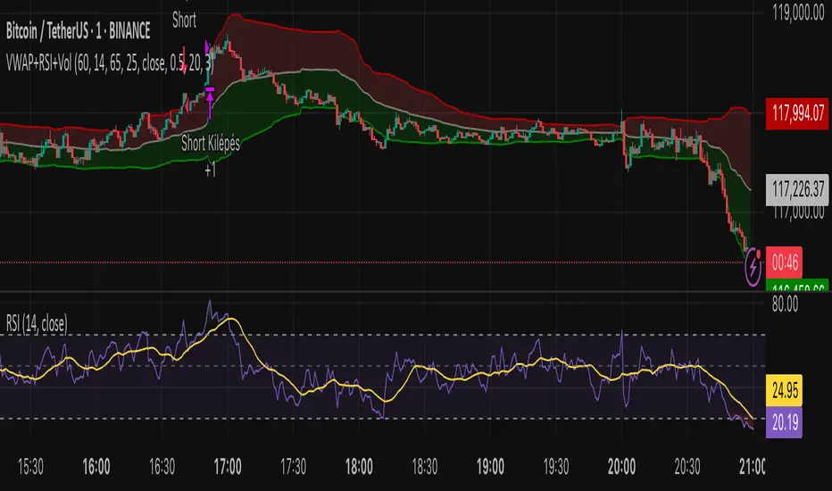
[Stratégia] VWAP Mean Magnet v9 (Simple Alert)This strategy is specifically designed for a ranging (sideways-moving) Bitcoin market.
A trade is only opened and signaled on the chart if all three of the following conditions are met simultaneously at the close of a candle:
Zone Entry
The price must cross into the signal zone: the red band for a Short (sell) position, or the green band for a Long (buy) position.
RSI Confirmation
The RSI indicator must also confirm the signal. For a Short, it must go above 65 (overbought condition). For a Long, it must fall below 25 (oversold condition).
Volume Filter
The volume on the entry candle cannot be excessively high. This safety filter is designed to prevent trades during risky, high-momentum breakouts.
Bande e canali

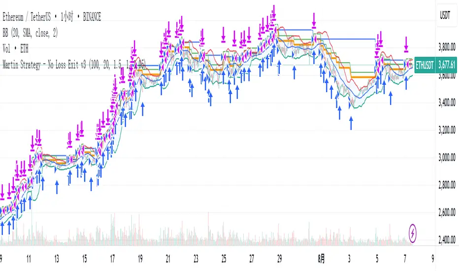
Martin Strategy - No Loss Exit v3Martin Strategy - No Loss Exit v3Martin Strategy - No Loss Exit v3Martin Strategy - No Loss Exit v3
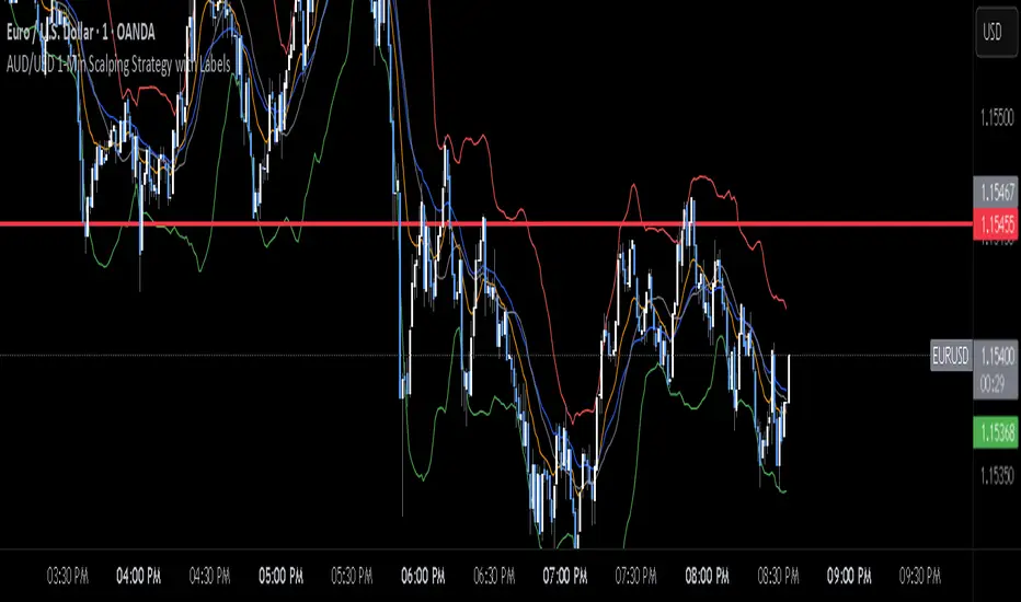
AUD/USD 1-Min Scalping Strategy with LabelsHere’s a complete TradingView Pine Script v5 for the 1-minute AUD/USD scalping strategy we just discussed. This strategy uses:
EMA 13 and EMA 26 for trend filtering
Bollinger Bands for volatility extremes
RSI (4) for momentum confirmation
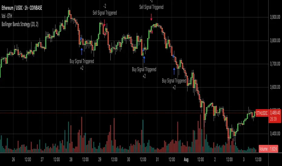
Bollinger Bands SMA 20_2 StrategyMean reversion strategy using Bollinger Bands (20-period SMA with 2.0 standard deviation bands).
Trade Triggers:
🟢 BUY SIGNAL:
When: Price crosses above the lower Bollinger Band
Logic: Price has hit oversold territory and is bouncing back
Action: Places a long position with stop at the lower band
🔴 SELL SIGNAL:
When: Price crosses below the upper Bollinger Band
Logic: Price has hit overbought territory and is pulling back
Action: Places a short position with stop at the upper band
TOT Strategy, The ORB Titan (Configurable)This is a strategy script adapted from Deniscr 's indicator script found here:
All feedback welcome!

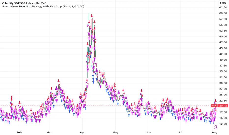
Linear Mean Reversion Strategy📘 Strategy Introduction: Linear Mean Reversion with Fixed Stop
This strategy implements a simple yet powerful mean reversion model that assumes price tends to oscillate around a dynamic average over time. It identifies statistically significant deviations from the moving average using a z-score, and enters trades expecting a return to the mean.
🧠 Core Logic:
A z-score is calculated by comparing the current price to its moving average, normalized by standard deviation, over a user-defined half-life window.
Trades are entered when the z-score crosses a threshold (e.g., ±1), signaling overbought or oversold conditions.
The strategy exits positions either when price reverts back near the mean (z-score close to 0), or if a fixed stop loss of 100 points is hit, whichever comes first.
⚙️ Key Features:
Dynamic mean and volatility estimation using moving average and standard deviation
Configurable z-score thresholds for entry and exit
Position size scaling based on z-score magnitude
Fixed stop loss to control risk and avoid prolonged drawdowns
🧪 Use Case:
Ideal for range-bound markets or assets that exhibit stationary behavior around a mean, this strategy is especially useful on assets with mean-reverting characteristics like currency pairs, ETFs, or large-cap stocks. It is best suited for traders looking for short-term reversions rather than long-term trends.
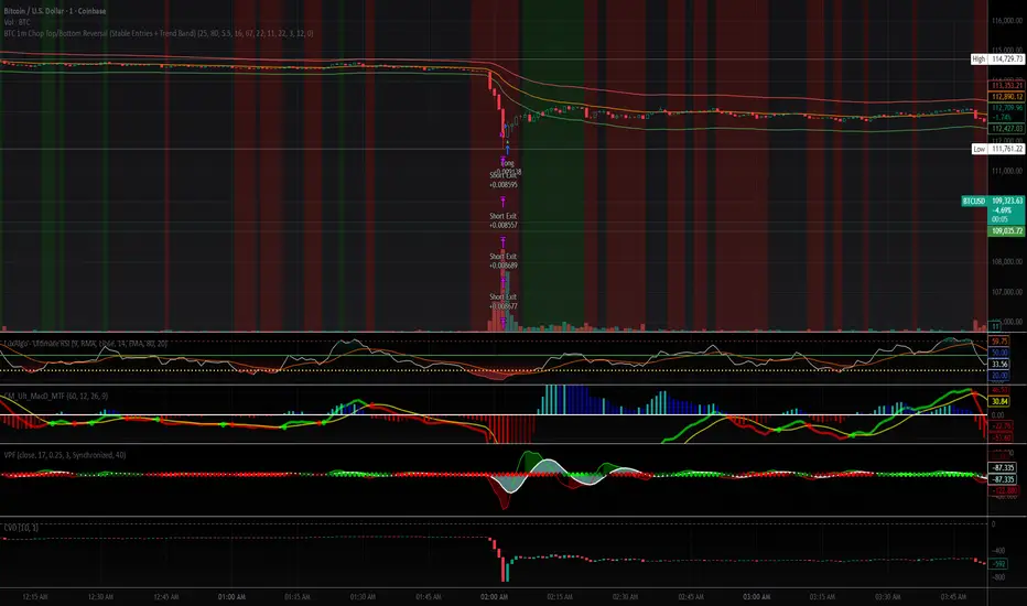
BTC 1m Chop Top/Bottom Reversal (Stable Entries)Strategy Description: BTC 5m Chop Top/Bottom Reversal (Stable Entries)
This strategy is engineered to capture precise reversal points during Bitcoin’s choppy or sideways price action on the 5-minute timeframe. It identifies short-term tops and bottoms using a confluence of volatility bands, momentum indicators, and price structure, optimized for high-probability scalping and intraday reversals.
Core Logic:
Volatility Filter: Uses an EMA with ATR bands to define overextended price zones.
Momentum Divergence: Confirms reversals using RSI and MACD histogram shifts.
Price Action Filter: Requires candle confirmation in the direction of the trade.
Locked Signal Logic: Prevents repaints and disappearing trades by confirming signals only once per bar.
Trade Parameters:
Short Entry: Above upper band + overbought RSI + weakening MACD + bearish candle
Long Entry: Below lower band + oversold RSI + strengthening MACD + bullish candle
Take Profit: ±0.75%
Stop Loss: ±0.4%
This setup is tuned for traders using tight risk control and leverage, where execution precision and minimal drawdown tolerance are critical.
Dubic EMA StrategyThe Dubic EMA Strategy is a trend-following and volatility-aware strategy that combines dual EMA filters with intelligent range and noise detection to provide clean, actionable entries. It's designed to avoid choppy markets, enhance trade precision, and adapt to different market conditions.
✅ Key Features:
Dual EMA Filter: Enters long when price is above both EMA High & EMA Low, and short when below both.
Range Filter: Avoids entries during tight consolidations or sideways markets.
Volatility Filter: Prevents trading in low-ATR conditions.
Dynamic Risk Management:
ATR-based or fixed % Stop Loss and Take Profit.
Optional Parabolic SAR trailing stop.
One Trade per Trend: Prevents re-entry until trend direction changes.
Unbroken Range Visualization: Detects and displays consolidation zones that can lead to breakouts.
Alerts & Labels: Clean BUY/SELL signals with alerts and chart labels.
🧩 Customization Options:
Adjustable EMA length
Toggle between ATR or % based SL/TP
Volatility threshold
Range detection sensitivity
Enable/disable SAR trailing stop
This strategy works best on trending assets and timeframes with volatility (e.g., crypto, forex, indices). Suitable for both manual trading and automation.
🛠️ Built for clarity, control, and precision.
📈 Backtest, optimize, and deploy with confidence.

[Stratégia] VWAP Mean Magnet v2 (VolSzűrő)Ez a stratégia BTC- oldalazó időszakára van kifejlestve 1 perces chartra.
4H Bollinger Breakout StrategyThis strategy leverages Bollinger Bands on the 4-hour timeframe for long and short trades in trending or ranging markets. Entries trigger on BB breakouts with optional filters for volume, trend, and RSI. Exits occur on opposite BB crosses. Customizable for long-only, short-only, or indicator mode via code comments. Supports forex, stocks, or crypto with full equity allocation and 0.1% commission.
Length (Default: 20): Period for BB basis and std dev; shorter for sensitivity, longer for smoothing.
Basis MA Type (Default: SMA): Selects MA for middle band (SMA, EMA, etc.); EMA for faster response.
Source (Default: Close): Price input for calculations; use close for standard accuracy.
StdDev Multiplier (Default: 1.8): Band width control; higher for fewer signals, lower for more.
Offset (Default: 0): Shifts BB plots; typically unchanged.
Use Filters (Default: True): Applies volume, trend, RSI checks to filter signals.
Volume MA Length (Default: 20): For volume filter (long: >105% avg, short: >120%).
Trend MA Length (Default: 80): SMA for trend filter (long: above MA, short: below).
RSI Length (Default: 14): For short filter (entry if RSI <85).
Use Long/Short Signals (Defaults: True): Toggles directions; long entry on lower BB crossover, short on upper crossunder.
Visuals: BB plots (blue basis, red upper, green lower), orange trend MA, filled background.
Labels/Alerts: Green/red for long entry/exit, yellow/purple for short; alert conditions included.

Combo 2/20 EMA & Bandpass Filter by TamarokDescription:
This strategy combines a 2/20 exponential moving average (EMA) crossover with a custom bandpass filter to generate buy and sell signals.
Use the Fast EMA and Slow EMA inputs to adjust trend sensitivity, and the Bandpass Filter Length, Delta, and Zones to fine-tune momentum turns.
Signals occur when both EMA and BPF agree in direction, with optional reversal and time filters.
How to use:
1. Add the script to your chart in TradingView.
2. Adjust the EMA and BP Filter parameters to match your asset’s volatility.
3. Enable ‘Reverse Signals’ to trade counter-trend, or use the time filter to limit sessions.
4. Set alerts on Long Alert and Short Alert for automated notifications.
Inspiration:
Based on HPotter’s original combo strategy (Stocks & Commodities Mar 2010).
Updated to Pine Script v6 with streamlined code and alerts.
WARNING:
For purpose educate only

Opening-Range BreakoutNote: Default trading date range looks mediocre. Set date range to "Entire History" to see full effect of the strategy. 50.91% profitable trades, 1.178 profit factor, steady profits and limited drawdown. Total P&L: $154,141.18, Max Drawdown: $18,624.36. High R^2
█ Overview
The Opening-Range Breakout strategy is a mechanical, session‑based day‑trading system designed to capture the initial burst of directional momentum immediately following the market open. It defines a user‑configurable “opening range” window, measures its high and low boundaries, then places breakout stop orders at those levels once the range closes. Built‑in filters on minimum range width, reward‑to‑risk ratios, and optional reversal logic help refine entries and manage risk dynamically.
█ How It Works
Opening‑Range Formation
Between 9:30–10:15 AM ET (configurable), the script tracks the highest high and lowest low to form the day’s opening range box.
On the first bar after the range window closes, the range high (OR_high) and low (OR_low) are “locked in.”
Range‑Width Filter
To avoid false breakouts in low‑volatility mornings, the range must be at least X% of the current price (default 0.35%).
If the measured opening-range width < minimum threshold, no orders are placed that day.
Entry & Order Placement
Long: a stop‑buy order at the opening‑range high.
Short: a stop‑sell order at the opening‑range low.
Only one side can trigger (or both if reverse logic is enabled after a losing trade).
Risk Management
Once triggered, each trade uses an ATR‑style stop-loss defined as a percentage retracement of the range (default 50% of range width).
Profit target is set at a configurable Reward/Risk Ratio (default 1.1×).
Optional: Reverse on Stop‑Loss – if the initial breakout loses, immediately reverse into the opposite side on the same day.
Session Exit
Any open positions are closed at the end of the regular trading day (default 3:45 PM ET window end, with hard flat at session close).
Visual cues are provided via green (range high) and red (range low) step‑line plots directly on the chart, allowing you to see the range box and breakout triggers in real time.
█ Why It Works
Early Momentum Capture: The first 15 – 60 minutes of trading encapsulate overnight news digestion and institutional order flow, creating a well‑defined volatility “range.”
Mechanical Discipline: Clear, rule‑based entries and exits remove emotional guesswork, ensuring consistency.
Volatility Filtering: By requiring a minimum range width, the system avoids choppy, low‑range days where false breakouts are common.
Dynamic Sizing: Stops and targets scale with the opening range, adapting automatically to each day’s volatility environment.
█ How to Use
Set Your Instruments & Timeframe
-Apply to any futures contract on a 1‑ to 5‑minute chart.
-Ensure chart timezone is set to America/New_York.
Configure Inputs
-Opening‑Range Window: e.g. “0930-1015” for a 45‑minute range.
-Min. OR Width (%): e.g. 0.35 for 0.35% of current price.
-Reward/Risk Ratio: e.g. 1.1 for a modest profit target above your stop.
-Max OR Retracement %: e.g. 50 to set stop at 50% of range width.
-One Trade Per Day: toggle to limit to a single breakout.
-Reverse on Stop Loss: toggle to flip direction after a losing breakout.
Monitor the Chart
-Watch the green and red range boundaries form during the session open.
-Orders will automatically submit on the first bar after the range window closes, conditioned on your filters.
Review & Adjust
-Backtest across multiple months to validate performance on your preferred contract.
-Tweak range duration, minimum width, and R/R multiple to fit your risk tolerance and desired win‑rate vs. expectancy balance.
█ Settings Reference
Input Defaults
Opening‑Range Window - Time window to form OR (HHMM-HHMM) - 0930–1015
Regular Trading Day - Full session for EOD flat (HHMM-HHMM) - 0930–1545
Min. OR Width (%) - Minimum OR size as % of close to trigger orders - 0.35
Reward/Risk Ratio - Profit target multiple of stop‑loss distance - 1.1
Max OR Retracement (%) - % of OR width to use as stop‑loss distance - 50
One Trade Per Day - Limit to a single breakout order per day - false
Reverse on Stop Loss - Reverse direction immediately after a losing trade - true
Disclaimer
This strategy description and any accompanying code are provided for educational purposes only and do not constitute financial advice or a solicitation to trade. Futures trading involves substantial risk, including possible loss of capital. Past performance is not indicative of future results. Traders should assess their own risk tolerance and conduct thorough backtesting and forward-testing before committing real capital.

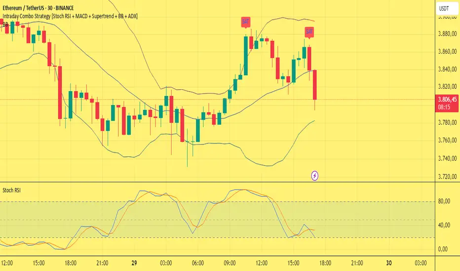
Intraday Combo Strategy HHStochastic RSI Momentum/Reversal quickly identifies overbought/oversold zones
MACD Momentum/Trend confirms a trend reversal, a late but powerful signal
Supertrend Trend Tracking provides clear and concise buy/sell signals
Bollinger Bands Volatility shows price deviation during breakouts/squeezes
ADX Trend Strength measures trend strength to filter out false signals
Setup: Smooth Gaussian + Adaptive Supertrend (Manual Vol)Overview
This strategy combines two powerful trend-based tools originally developed by Algo Alpha: the Smooth Gaussian Trend (simulated) and the Adaptive Supertrend. The objective is to capture sustained bullish movements in periods of controlled volatility by filtering for high-probability entries.
Entry Logic
Long Entry Conditions:
The closing price is above the Smooth Gaussian Trend line (with length = 75), and
The volatility setting from the Adaptive Supertrend is manually defined as either 2 or 3
Exit Condition:
The closing price falls below the Smooth Gaussian Trend line
This script uses a simulated version of the Gaussian Trend line via double-smoothed SMA, as the original Algo Alpha indicator is protected and cannot be accessed directly in code.
Features
Plots entry and exit signals directly on the chart
Manual toggle to enable or disable the volatility filter
Lightweight design to allow flexible backtesting even without access to proprietary indicators
Important Note
This strategy does not connect to the actual Adaptive Supertrend from Algo Alpha. Users must manually input the volatility level based on what they observe on the chart when the original indicator is also applied. The Smooth Gaussian Trend is approximated and may differ slightly from the original.
Suggested Use
Recommended timeframes: 1H, 4H, or Daily
Best used alongside the original indicators displayed on the chart
Consider incorporating additional structure, momentum, or volume filters to enhance performance
If you have suggestions or would like to contribute improvements, feel free to reach out or fork the script.

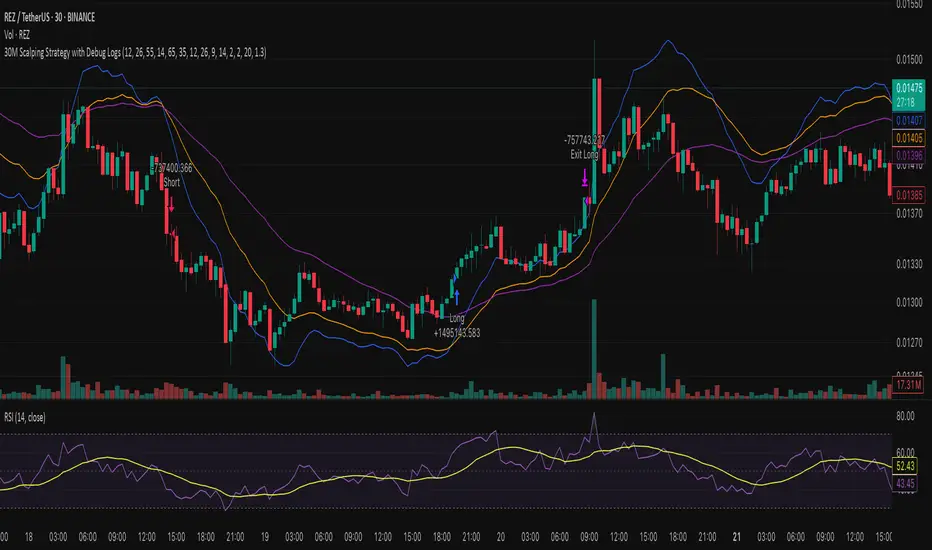
30M Scalping Strategy with Debug LogsWhat’s changed
Spot‑only: all short logic removed—only long entries and exits are generated.
Logging: uses log.info() to send entry/exit details (timestamp, price, ATR, RSI) to the Pine Logs console.
Clean & concise: core scalp logic (EMAs, RSI, MACD, volume, ATR SL/TP) remains intact.
EMA 20 and Anchored VWAP with Typical PriceIntraday scalping using EMA 20 and VWAP along with targets and Stoploss
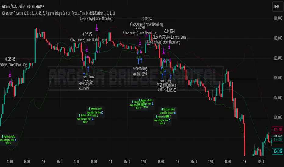
Quantum Reversal# 🧠 Quantum Reversal
## **Quantitative Mean Reversion Framework**
This algorithmic trading system employs **statistical mean reversion theory** combined with **adaptive volatility modeling** to capitalize on Bitcoin's inherent price oscillations around its statistical mean. The strategy integrates multiple technical indicators through a **multi-layered signal processing architecture**.
---
## ⚡ **Core Technical Architecture**
### 📊 **Statistical Foundation**
- **Bollinger Band Mean Reversion Model**: Utilizes 20-period moving average with 2.2 standard deviation bands for volatility-adjusted entry signals
- **Adaptive Volatility Threshold**: Dynamic standard deviation multiplier accounts for Bitcoin's heteroscedastic volatility patterns
- **Price Action Confluence**: Entry triggered when price breaches lower volatility band, indicating statistical oversold conditions
### 🔬 **Momentum Analysis Layer**
- **RSI Oscillator Integration**: 14-period Relative Strength Index with modified oversold threshold at 45
- **Signal Smoothing Algorithm**: 5-period simple moving average applied to RSI reduces noise and false signals
- **Momentum Divergence Detection**: Captures mean reversion opportunities when momentum indicators show oversold readings
### ⚙️ **Entry Logic Architecture**
```
Entry Condition = (Price ≤ Lower_BB) OR (Smoothed_RSI < 45)
```
- **Dual-Condition Framework**: Either statistical price deviation OR momentum oversold condition triggers entry
- **Boolean Logic Gate**: OR-based entry system increases signal frequency while maintaining statistical validity
- **Position Sizing**: Fixed 10% equity allocation per trade for consistent risk exposure
### 🎯 **Exit Strategy Optimization**
- **Profit-Lock Mechanism**: Positions only closed when showing positive unrealized P&L
- **Trend Continuation Logic**: Allows winning trades to run until momentum exhaustion
- **Dynamic Exit Timing**: No fixed profit targets - exits based on profitability state rather than arbitrary levels
---
## 📈 **Statistical Properties**
### **Risk Management Framework**
- **Long-Only Exposure**: Eliminates short-squeeze risk inherent in cryptocurrency markets
- **Mean Reversion Bias**: Exploits Bitcoin's tendency to revert to statistical mean after extreme moves
- **Position Management**: Single position limit prevents over-leveraging
### **Signal Processing Characteristics**
- **Noise Reduction**: SMA smoothing on RSI eliminates high-frequency oscillations
- **Volatility Adaptation**: Bollinger Bands automatically adjust to changing market volatility
- **Multi-Timeframe Coherence**: Indicators operate on consistent timeframe for signal alignment
---
## 🔧 **Parameter Configuration**
| Technical Parameter | Value | Statistical Significance |
|-------------------|-------|-------------------------|
| Bollinger Period | 20 | Standard statistical lookback for volatility calculation |
| Std Dev Multiplier | 2.2 | Optimized for Bitcoin's volatility distribution (95.4% confidence interval) |
| RSI Period | 14 | Traditional momentum oscillator period |
| RSI Threshold | 45 | Modified oversold level accounting for Bitcoin's momentum characteristics |
| Smoothing Period | 5 | Noise reduction filter for momentum signals |
---
## 📊 **Algorithmic Advantages**
✅ **Statistical Edge**: Exploits documented mean reversion tendency in Bitcoin markets
✅ **Volatility Adaptation**: Dynamic bands adjust to changing market conditions
✅ **Signal Confluence**: Multiple indicator confirmation reduces false positives
✅ **Momentum Integration**: RSI smoothing improves signal quality and timing
✅ **Risk-Controlled Exposure**: Systematic position sizing and long-only bias
---
## 🔬 **Mathematical Foundation**
The strategy leverages **Bollinger Band theory** (developed by John Bollinger) which assumes that prices tend to revert to the mean after extreme deviations. The RSI component adds **momentum confirmation** to the statistical price deviation signal.
**Statistical Basis:**
- Mean reversion follows the principle that extreme price deviations from the moving average are temporary
- The 2.2 standard deviation multiplier captures approximately 97.2% of price movements under normal distribution
- RSI momentum smoothing reduces noise inherent in oscillator calculations
---
## ⚠️ **Risk Considerations**
This algorithm is designed for traders with understanding of **quantitative finance principles** and **cryptocurrency market dynamics**. The strategy assumes mean-reverting behavior which may not persist during trending market phases. Proper risk management and position sizing are essential.
---
## 🎯 **Implementation Notes**
- **Market Regime Awareness**: Most effective in ranging/consolidating markets
- **Volatility Sensitivity**: Performance may vary during extreme volatility events
- **Backtesting Recommended**: Historical performance analysis advised before live implementation
- **Capital Allocation**: 10% per trade sizing assumes diversified portfolio approach
---
**Engineered for quantitative traders seeking systematic mean reversion exposure in Bitcoin markets through statistically-grounded technical analysis.**
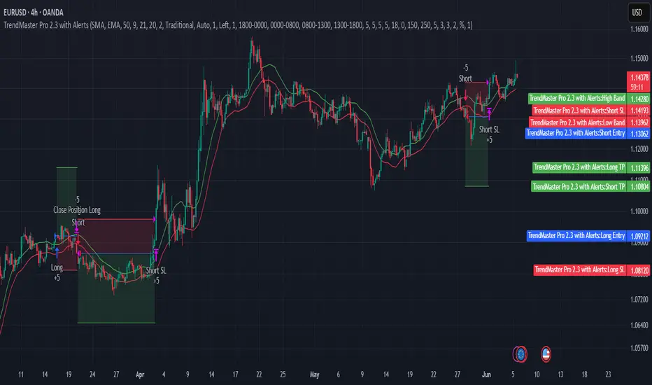
TrendMaster Pro 2.3 with Alerts
Hello friends,
A member of the community approached me and asked me how to write an indicator that would achieve a particular set of goals involving comprehensive trend analysis, risk management, and session-based trading controls. Here is one example method of how to create such a system:
Core Strategy Components
Multi-Moving Average System - Uses configurable MA types (EMA, SMA, SMMA) with short-term (9) and long-term (21) periods for primary signal generation through crossovers
Higher Timeframe Trend Filter - Optional trend confirmation using a separate MA (default 50-period) to ensure trades align with broader market direction
Band Power Indicator - Dynamic high/low bands calculated using different MA types to identify price channels and volatility zones
Advanced Signal Filtering
Bollinger Bands Volatility Filter - Prevents trading during low-volatility ranging markets by requiring sufficient band width
RSI Momentum Filter - Uses customizable thresholds (55 for longs, 45 for shorts) to confirm momentum direction
MACD Trend Confirmation - Ensures MACD line position relative to signal line aligns with trade direction
Stochastic Oscillator - Adds momentum confirmation with overbought/oversold levels
ADX Strength Filter - Only allows trades when trend strength exceeds 25 threshold
Session-Based Trading Management
Four Trading Sessions - Asia (18:00-00:00), London (00:00-08:00), NY AM (08:00-13:00), NY PM (13:00-18:00)
Individual Session Limits - Separate maximum trade counts for each session (default 5 per session)
Automatic Session Closure - All positions close at specified market close time
Risk Management Features
Multiple Stop Loss Options - Percentage-based, MA cross, or band-based SL methods
Risk/Reward Ratio - Configurable TP levels based on SL distance (default 1:2)
Auto-Risk Calculation - Dynamic position sizing based on dollar risk limits ($150-$250 range)
Daily Limits - Stop trading after reaching specified TP or SL counts per day
Support & Resistance System
Multiple Pivot Types - Traditional, Fibonacci, Woodie, Classic, DM, and Camarilla calculations
Flexible Timeframes - Auto-adjusting or manual timeframe selection for S/R levels
Historical Levels - Configurable number of past S/R levels to display
Visual Customization - Individual color and display settings for each S/R level
Additional Features
Alert System - Customizable buy/sell alert messages with once-per-bar frequency
Visual Trade Management - Color-coded entry, SL, and TP levels with fill areas
Session Highlighting - Optional background colors for different trading sessions
Comprehensive Filtering - All signals must pass through multiple confirmation layers before execution
This approach demonstrates how to build a professional-grade trading system that combines multiple technical analysis methods with robust risk management and session-based controls, suitable for algorithmic trading across different market sessions.
Good luck and stay safe!
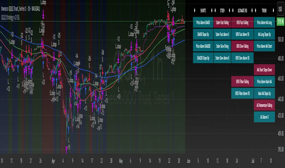
QQQ Strategy v2 ESL | easy-peasy-x This is a strategy optimized for QQQ (and SPY) for the 1H timeframe. It significantly outperforms passive buy-and-hold approach. With settings adjustments, it can be used on various assets like stocks and cryptos and various timeframes, although the default out of the box settings favor QQQ 1H.
The strategy uses various triggers to take both long and short trades. These can be adjusted in settings. If you try a different asset, see what combination of triggers works best for you.
Some of the triggers employ LuxAlgo's Ultimate RSI - shoutout to him for great script, check it out here .
Other triggers are based on custom signed standard deviation - basically the idea is to trade Bollinger Bands expansions (long to the upside, short to the downside) and fade or stay out of contractions.
There are three key moving averages in the strategy - LONG MA, SHORT MA, BASIC MA. Long and Short MAs are guides to eyes on the chart and also act as possible trend filters (adjustable in settings). Basic MA acts as guide to eye and a possible trade trigger (adjustable in settings).
There are a few trend filters the strategy can use - moving average, signed standard deviation, ultimate RSI or none. The filters act as an additional condition on triggers, making the strategy take trades only if both triggers and trend filter allows. That way one can filter out trades with unfavorable risk/reward (for instance, don't long if price is under the MA200). Different trade filters can be used for long and short trades.
The strategy employs various stop loss types, the default of which is a trailing %-based stop loss type. ATR-based stop loss is also available. The default 1.5% trailing stop loss is suitable for leveraged trading.
Lastly, the strategy can trigger take profit orders if certain conditions are met, adjustable in settings. Also, it can hold onto winning trades and exit only after stop out (in which case, consecutive triggers to take other positions will be ignored until stop out).
Let me know if you like it and if you use it, what kind of tweaks would you like to see.
With kind regards,
easy-peasy-x
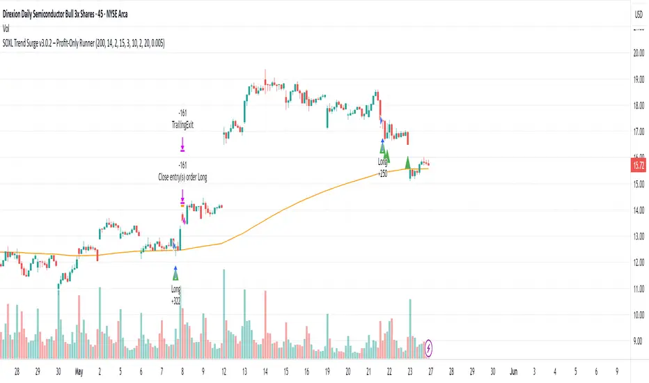
SOXL Trend Surge v3.0.2 – Profit-Only RunnerSOXL Trend Surge v3.0.2 – Profit-Only Runner
This is a trend-following strategy built for leveraged ETFs like SOXL, designed to ride high-momentum waves with minimal interference. Unlike most short-term scalping scripts, this model allows trades to develop over multiple days to even several months, capitalizing on the full power of extended directional moves — all without using a stop-loss.
🔍 How It Works
Entry Logic:
Price is above the 200 EMA (long-term trend confirmation)
Supertrend is bullish (momentum confirmation)
ATR is rising (volatility expansion)
Volume is above its 20-bar average (liquidity filter)
Price is outside a small buffer zone from the 200 EMA (to avoid whipsaws)
Trades are restricted to market hours only (9 AM to 2 PM EST)
Cooldown of 15 bars after each exit to prevent overtrading
Exit Strategy:
Takes partial profit at +2× ATR if held for at least 2 bars
Rides the remaining position with a trailing stop at 1.5× ATR
No hard stop-loss — giving space for volatile pullbacks
⚙️ Strategy Settings
Initial Capital: $500
Risk per Trade: 100% of equity (fully allocated per entry)
Commission: 0.1%
Slippage: 1 tick
Recalculate after order is filled
Fill orders on bar close
Timeframe Optimized For: 45-minute chart
These parameters simulate an aggressive, high-volatility trading model meant for forward-testing compounding potential under realistic trading costs.
✅ What Makes This Unique
No stop-loss = fewer premature exits
Partial profit-taking helps lock in early wins
Trailing logic gives room to ride large multi-week moves
Uses strict filters (volume, ATR, EMA bias) to enter only during high-probability windows
Ideal for leveraged ETF swing or position traders looking to hold longer than the typical intraday or 2–3 day strategies
⚠️ Important Note
This is a high-risk, high-reward strategy meant for educational and testing purposes. Without a stop-loss, trades can experience deep drawdowns that may take weeks or even months to recover. Always test thoroughly and adjust position sizing to suit your risk tolerance. Past results do not guarantee future returns. Backtest range: May 8, 2020 – May 23, 2025
Range Filter Strategy with ATR TP/SLHow This Strategy Works:
Range Filter:
Calculates a smoothed average (SMA) of price
Creates upper and lower bands based on standard deviation
When price crosses above upper band, it signals a potential uptrend
When price crosses below lower band, it signals a potential downtrend
ATR-Based Risk Management:
Uses Average True Range (ATR) to set dynamic take profit and stop loss levels
Take profit is set at entry price + (ATR × multiplier) for long positions
Stop loss is set at entry price - (ATR × multiplier) for long positions
The opposite applies for short positions
Input Parameters:
Adjustable range filter length and multiplier
Customizable ATR length and TP/SL multipliers
All parameters can be optimized in TradingView's strategy tester
You can adjust the input parameters to fit your trading style and the specific market you're trading. The ATR-based exits help adapt to current market volatility.

Big Mover Catcher BTC 4h🧠 Big Mover Catcher (BTC 4H Strategy) — Educational Tool
⚠️ Disclaimer: I am not a financial advisor. This script is for educational and testing purposes only. Cryptocurrency trading is highly volatile and involves significant risk. You can lose all of your invested capital.
📌 Overview
The Big Mover Catcher strategy is a work-in-progress trading system designed for Bitcoin (BTC) on the 4-hour chart. It aims to identify strong breakout moves by combining multiple technical indicators and conditions, allowing for high customization and filter-based confirmations.
This script is part of a personal project to learn Pine Script and backtesting on TradingView. It is currently in the testing and research phase.
🎯 Strategy Objective
Catch large, high-momentum breakout moves in the BTC market using:
Bollinger Band breakouts for entry signals
Momentum, volatility, and trend filters for trade confirmation
🧰 Features & Filters
The script provides a flexible set of filters that can be turned ON/OFF and adjusted directly from the settings panel:
✅ Entry Conditions
Price must break above or below Bollinger Bands
All selected filters must align before entry
🧪 Available Filters:
Relative Strength Index (RSI) with EMA/SMA smoothing
Average Directional Index (ADX) with EMA/SMA smoothing
Average True Range (ATR) with EMA/SMA smoothing
MACD Signal above or below zero
EMA 350 trend filter
ATR / ADX / RSI Threshold toggles for added control
🔥 Additional Feature:
Force Take Profit: Optionally closes the trade immediately if a candle closes with more than a defined % movement (default: 5%). This can help lock in quick profits during high volatility moves.
⚙️ Customizable Inputs
You can configure:
Stop loss percentage
All indicator lengths
Smoothing types (EMA/SMA)
Threshold activation toggles
Individual filter ON/OFF switches
This makes the strategy highly adaptable for educational exploration and optimization.
📊 Best Used For
Learning Pine Script and strategy structure
Testing filter combinations for BTC on the 4H timeframe
Understanding how different indicators interact in live markets
⚠️ Note: ❌ Short trades are currently disabled by default, as short-side logic is still under development.
❗ Final Reminder
This script is not financial advice. It is an educational tool. Use it to learn and explore trading logic. Trading cryptocurrencies carries high risk — only invest what you can afford to lose.