Estrategia Momentum Seguro (EMS) Entry and exit signals, this indicator helps or suggests where to enter, exit, or place a stop loss.
Analisi fondamentale

1M XAU Cumulative Delta Volume with OB Breakouts
### Overview
This is a **session-based CVD strategy** built around the **00:00–07:00 CEST range**. It finds the high/low of that session, turns them into **adaptive ATR-based support (yellow)** and **resistance (purple)** zones, and trades only **CVD-confirmed reversals** off those levels.
---
### How it Works
* For each day, the script:
* Builds a 00:00–07:00 CEST **profile high/low**.
* Creates a **support zone** around the session low and a **resistance zone** around the session high.
* Using lower timeframe data, it reconstructs **Cumulative Volume Delta (CVD)** and a **recent delta** filter.
* It arms “pending” states when price **enters a zone from the correct side**, then confirms:
* **BUY (long):** price reclaims above support and recent CVD is strongly positive.
* **SELL (short):** price rejects below resistance and recent CVD is strongly negative.
Only these two CVD signals (`buySignal` / `sellSignal`) open trades.
---
### Strategy Logic
* **Entries**
* `buySignal` → open **long** (if flat).
* `sellSignal` → open **short** (if flat).
* No pyramiding; one position at a time.
* **Exits (only TP & SL)**
* Long: TP at `avg_price * (0.5 + TP%)`, SL at `avg_price * (1 – SL%)`.
* Short: TP at `avg_price * (0.5 – TP%)`, SL at `avg_price * (1 + SL%)`.
* No opposite-signal exits.
---
### Extras
* **Reversal markers** on yellow/purple zones and **breakout/retest markers** are plotted for context and alerts but **do not trigger entries**.
* Zone width and “thickening” are ATR-based so important touches and near-touches are easy to see.
* Only suited for **1m intraday scalping** (e.g. XAU/USD), but can be tested on other markets/timeframes.

Pivot Fib 4H — EAStrategy uses the pivot standard to open position, it has well define entry and exit point with SL, it also has a proper money management plan, maximum 4 trades a day, each trade risk 0.5% of the account, I have it EA version of it also.

Liquidity Sweep + BOS Retest System — Prop Firm Edition🟦 Liquidity Sweep + BOS Retest System — Prop Firm Edition
A High-Probability Smart Money Strategy Built for NQ, ES, and Funding Accounts
🚀 Overview
The Liquidity Sweep + BOS Retest System (Prop Firm Edition) is a precision-engineered SMC strategy built specifically for prop firm traders. It mirrors institutional liquidity behavior and combines it with strict account-safe entry rules to help traders pass and maintain funding accounts with consistency.
Unlike typical indicators, this system waits for three confirmations — liquidity sweep, displacement, and a clean retest — before executing any trade. Every component is optimized for low drawdown, high R:R, and prop-firm-approved risk management.
Whether you’re trading Apex, TakeProfitTrader, FFF, or OneUp Trader, this system gives you a powerful mechanical framework that keeps you within rules while identifying the market’s highest-probability reversal zones.
🔥 Key Features
1. Liquidity Sweep Detection (Stop Hunt Logic)
Automatically identifies when price clears a previous swing high/low with a sweep confirmation candle.
✔ Filters noise
✔ Eliminates early entries
✔ Locks onto true liquidity grabs
2. Automatic Break of Structure (BOS) Confirmation
Price must show true displacement by breaking structure opposite the sweep direction.
✔ Confirms momentum shift
✔ Removes fake reversals
✔ Ensures institutional intent
3. Precision Retest Entry Model
The strategy enters only when price retests the BOS level at premium/discount pricing.
✔ Zero chasing
✔ Extremely tight stop loss placement
✔ Prop-firm-friendly controlled risk
4. Built-In Risk & Trade Management
SL set at swept liquidity
TP set by user-defined R:R multiplier
Optional session filter (NY Open by default)
One trade at a time (no pyramiding)
Automatically resets logic after each trade
This prevents overtrading — the #1 cause of evaluation and account breaches.
5. Designed for Prop Firm Futures Trading
This script is optimized for:
Trailing/static drawdown accounts
Micro contract precision
Funding evaluations
Low-risk, high-probability setups
Structured, rule-based execution
It reduces randomness and emotional trading by automating the highest-quality SMC sequence.
🎯 The Trading Model Behind the System
Step 1 — Liquidity Sweep
Price must take out a recent high/low and close back inside structure.
This confirms stop-hunting behavior and marks the beginning of a potential reversal.
Step 2 — BOS (Break of Structure)
Price must break the opposite side swing with a displacement candle. This validates a directional shift.
Step 3 — Retest Entry
The system waits for price to retrace into the BOS level and signal continuation.
This creates optimal R:R entry with minimal drawdown.
📈 Best Markets
NQ (NASDAQ Futures) – Highly recommended
ES, YM, RTY
Gold (XAUUSD)
FX majors
Crypto (with high volatility)
Works best on 1m, 2m, 5m, or 15m depending on your trading style.
🧠 Why Traders Love This System
✔ No signals until all confirmations align
✔ Reduces overtrading and emotional decisions
✔ Follows market structure instead of random indicators
✔ Perfect for maintaining long-term funded accounts
✔ Built around institutional-grade concepts
✔ Makes your trading consistent, calm, and rules-based
⚙️ Recommended Settings
Session: 06:30–08:00 MST (NY Open)
R:R: 1.5R – 3R
Contracts: Start with 1–2 micros
Markets: NQ for best structure & volume
📦 What’s Included
Complete strategy logic
All plots, labels, sweep markers & BOS alerts
BOS retest entry automation
Session filtering
Stop loss & take profit system
Full SMC logic pipeline
🏁 Summary
The Liquidity Sweep + BOS Retest System is a complete, prop-firm-ready, structure-based strategy that automates one of the cleanest and most reliable SMC entry models. It is designed to keep you safe, consistent, and rule-compliant while capturing premium institutional setups.
If you want to trade with confidence, discipline, and prop-firm precision — this system is for you.
Good Luck -BG

SP500 Session Gap Fade StrategySummary in one paragraph
SPX Session Gap Fade is an intraday gap fade strategy for index futures, designed around regular cash sessions on five minute charts. It helps you participate only when there is a full overnight or pre session gap and a valid intraday session window, instead of trading every open. The original part is the gap distance engine which anchors both stop and optional target to the previous session reference close at a configurable flat time, so every trade’s risk scales with the actual gap size rather than a fixed tick stop.
Scope and intent
• Markets. Primarily index futures such as ES, NQ, YM, and liquid index CFDs that exhibit overnight gaps and regular cash hours.
• Timeframes. Intraday timeframes from one minute to fifteen minutes. Default usage is five minute bars.
• Default demo used in the publication. Symbol CME:ES1! on a five minute chart.
• Purpose. Provide a simple, transparent way to trade opening gaps with a session anchored risk model and forced flat exit so you are not holding into the last part of the session.
• Limits. This is a strategy. Orders are simulated on standard candles only.
Originality and usefulness
• Unique concept or fusion. The core novelty is the combination of a strict “full gap” entry condition with a session anchored reference close and a gap distance based TP and SL engine. The stop and optional target are symmetric multiples of the actual gap distance from the previous session’s flat close, rather than fixed ticks.
• Failure mode it addresses. Fixed sized stops do not scale when gaps are unusually small or unusually large, which can either under risk or over risk the account. The session flat logic also reduces the chance of holding residual positions into late session liquidity and news.
• Testability. All key pieces are explicit in the Inputs: session window, minutes before session end, whether to use gap exits, whether TP or SL are active, and whether to allow candle based closes and forced flat. You can toggle each component and see how it changes entries and exits.
• Portable yardstick. The main unit is the absolute price gap between the entry bar open and the previous session reference close. tp_mult and sl_mult are multiples of that gap, which makes the risk model portable across contracts and volatility regimes.
Method overview in plain language
The strategy first defines a trading session using exchange time, for example 08:30 to 15:30 for ES day hours. It also defines a “flat” time a fixed number of minutes before session end. At the flat bar, any open position is closed and the bar’s close price is stored as the reference close for the next session. Inside the session, the strategy looks for a full gap bar relative to the prior bar: a gap down where today’s high is below yesterday’s low, or a gap up where today’s low is above yesterday’s high. A full gap down generates a long entry; a full gap up generates a short entry. If the gap risk engine is enabled and a valid reference close exists, the strategy measures the distance between the entry bar open and that reference close. It then sets a stop and optional target as configurable multiples of that gap distance and manages them with strategy.exit. Additional exits can be triggered by a candle color flip or by the forced flat time.
Base measures
• Range basis. The main unit is the absolute difference between the current entry bar open and the stored reference close from the previous session flat bar. That value is used as a “gap unit” and scaled by tp_mult and sl_mult to build the target and stop.
Components
• Component one: Gap Direction. Detects full gap up or full gap down by comparing the current high and low to the previous bar’s high and low. Gap down signals a long fade, gap up signals a short fade. There is no smoothing; it is a strict structural condition.
• Component two: Session Window. Only allows entries when the current time is within the configured session window. It also defines a flat time before the session end where positions are forced flat and the reference close is updated.
• Component three: Gap Distance Risk Engine. Computes the absolute distance between the entry open and the stored reference close. The stop and optional target are placed as entry ± gap_distance × multiplier so that risk scales with gap size.
• Optional component: Candle Exit. If enabled, a bullish bar closes short positions and a bearish bar closes long positions, which can shorten holding time when price reverses quickly inside the session.
• Session windows. Session logic uses the exchange time of the chart symbol. When changing symbols or venues, verify that the session time string still matches the new instrument’s cash hours.
Fusion rule
All gates are hard conditions rather than weighted scores. A trade can only open if the session window is active and the full gap condition is true. The gap distance engine only activates if a valid reference close exists and use_gap_risk is on. TP and SL are controlled by separate booleans so you can use SL only, TP only, or both. Long and short are symmetric by construction: long trades fade full gap downs, short trades fade full gap ups with mirrored TP and SL logic.
Signal rule
• Long entry. Inside the active session, when the current bar shows a full gap down relative to the previous bar (current high below prior low), the strategy opens a long position. If the gap risk engine is active, it places a gap based stop below the entry and an optional target above it.
• Short entry. Inside the active session, when the current bar shows a full gap up relative to the previous bar (current low above prior high), the strategy opens a short position. If the gap risk engine is active, it places a gap based stop above the entry and an optional target below it.
• Forced flat. At the configured flat time before session end, any open position is closed and the close price of that bar becomes the new reference close for the following session.
• Candle based exit. If enabled, a bearish bar closes longs, and a bullish bar closes shorts, regardless of where TP or SL sit, as long as a position is open.
What you will see on the chart
• Markers on entry bars. Standard strategy entry markers labeled “long” and “short” on the gap bars where trades open.
• Exit markers. Standard exit markers on bars where either the gap stop or target are hit, or where a candle exit or forced flat close occurs. Exit IDs “long_gap” and “short_gap” label gap based exits.
• Reference levels. Horizontal lines for the current long TP, long SL, short TP, and short SL while a position is open and the gap engine is enabled. They update when a new trade opens and disappear when flat.
• Session background. This version does not add background shading for the session; session logic runs internally based on time.
• No on chart table. All decisions are visible through orders and exit levels. Use the Strategy Tester for performance metrics.
Inputs with guidance
Session Settings
• Trading session (sess). Session window in exchange time. Typical value uses the regular cash session for each contract, for example “0830-1530” for ES. Adjust if your broker or symbol uses different hours.
• Minutes before session end to force exit (flat_before_min). Minutes before the session end where positions are forced flat and the reference close is stored. Typical range is 15 to 120. Raising it closes trades earlier in the day; lowering it allows trades later in the session.
Gap Risk
• Enable gap based TP/SL (use_gap_risk). Master switch for the gap distance exit engine. Turning it off keeps entries and forced flat logic but removes automatic TP and SL placement.
• Use TP limit from gap (use_gap_tp). Enables gap based profit targets. Typical values are true for structured exits or false if you want to manage exits manually and only keep a stop.
• Use SL stop from gap (use_gap_sl). Enables gap based stop losses. This should normally remain true so that each trade has a defined initial risk in ticks.
• TP multiplier of gap distance (tp_mult). Multiplier applied to the gap distance for the target. Typical range is 0.5 to 2.0. Raising it places the target further away and reduces hit frequency.
• SL multiplier of gap distance (sl_mult). Multiplier applied to the gap distance for the stop. Typical range is 0.5 to 2.0. Raising it widens the stop and increases risk per trade; lowering it tightens the stop and may increase the number of small losses.
Exit Controls
• Exit with candle logic (use_candle_exit). If true, closes shorts on bullish candles and longs on bearish candles. Useful when you want to react to intraday reversal bars even if TP or SL have not been reached.
• Force flat before session end (use_forced_flat). If true, guarantees you are flat by the configured flat time and updates the reference close. Turn this off only if you understand the impact on overnight risk.
Filters
There is no separate trend or volatility filter in this version. All trades depend on the presence of a full gap bar inside the session. If you need extra filtering such as ATR, volume, or higher timeframe bias, they should be added explicitly and documented in your own fork.
Usage recipes
Intraday conservative gap fade
• Timeframe. Five minute chart on ES regular session.
• Gap risk. use_gap_risk = true, use_gap_tp = true, use_gap_sl = true.
• Multipliers. tp_mult around 0.7 to 1.0 and sl_mult around 1.0.
• Exits. use_candle_exit = false, use_forced_flat = true. Focus on the structured TP and SL around the gap.
Intraday aggressive gap fade
• Timeframe. Five minute chart.
• Gap risk. use_gap_risk = true, use_gap_tp = false, use_gap_sl = true.
• Multipliers. sl_mult around 0.7 to 1.0.
• Exits. use_candle_exit = true, use_forced_flat = true. Entries fade full gaps, stops are tight, and candle color flips flatten trades early.
Higher timeframe gap tests
• Timeframe. Fifteen minute or sixty minute charts on instruments with regular gaps.
• Gap risk. Keep use_gap_risk = true. Consider slightly higher sl_mult if gaps are structurally wider on the higher timeframe.
• Note. Expect fewer trades and be careful with sample size; multi year data is recommended.
Properties visible in this publication
• On average our risk for each position over the last 200 trades is 0.4% with a max intraday loss of 1.5% of the total equity in this case of 100k $ with 1 contract ES. For other assets, recalculations and customizations has to be applied.
• Initial capital. 100 000.
• Base currency. USD.
• Default order size method. Fixed with size 1 contract.
• Pyramiding. 0.
• Commission. Flat 2 USD per order in the Strategy Tester Properties. (2$ buying + 2$selling)
• Slippage. One tick in the Strategy Tester Properties.
• Process orders on close. ON.
Realism and responsible publication
• No performance claims are made. Past results do not guarantee future outcomes.
• Costs use a realistic flat commission and one tick of slippage per trade for ES class futures.
• Default sizing with one contract on a 100 000 reference account targets modest per trade risk. In practice, extreme slippage or gap through events can exceed this, so treat the one and a half percent risk target as a design goal, not a guarantee.
• All orders are simulated on standard candles. Shapes can move while a bar is forming and settle on bar close.
Honest limitations and failure modes
• Economic releases, thin liquidity, and limit conditions can break the assumptions behind the simple gap model and lead to slippage or skipped fills.
• Symbols with very frequent or very large gaps may require adjusted multipliers or alternative risk handling, especially in high volatility regimes.
• Very quiet periods without clean gaps will produce few or no trades. This is expected behavior, not a bug.
• Session windows follow the exchange time of the chart. Always confirm that the configured session matches the symbol.
• When both the stop and target lie inside the same bar’s range, the TradingView engine decides which is hit first based on its internal intrabar assumptions. Without bar magnifier, tie handling is approximate.
Legal
Education and research only. This strategy is not investment advice. You remain responsible for all trading decisions. Always test on historical data and in simulation with realistic costs before considering any live use.

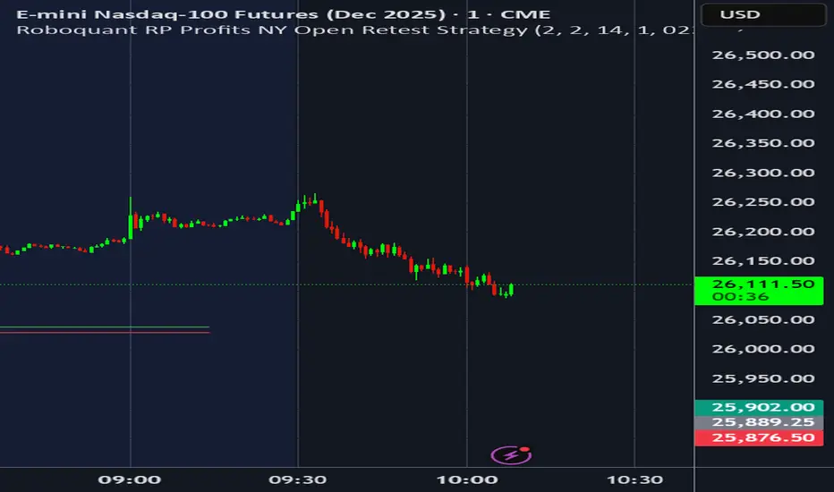
Roboquant RP Profits NY Open Retest StrategyRoboquant RP Profits NY Open Retest Strategy A good strategy for CL
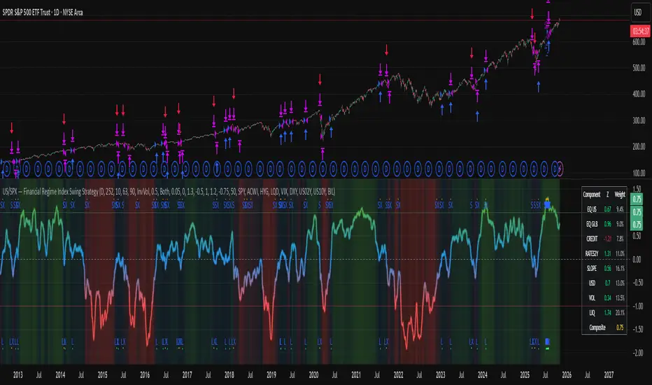
US/SPY- Financial Regime Index Swing Strategy Credits: concept inspired by EdgeTools Bloomberg Financial Conditions Index (Proxy)
Improvements: eight component basket, inverse volatility weights, winsorization option( statistical technique used to limit the influence of outliers in a dataset by replacing extreme values with less extreme ones, rather than removing them entirely), slope and price gates, exit guards, table and gradients.
Summary in one paragraph
A macro regime swing strategy for index ETFs, futures, FX majors, and large cap equities on daily calculation with optional lower time execution. It acts only when a composite Financial Conditions proxy plus slope and an optional price filter align. Originality comes from an eight component macro basket with inverse volatility weights and winsorized return z scores that produce a portable yardstick.
Scope and intent
Markets: SPY and peers, ES futures, ACWI, liquid FX majors, BTC, large cap equities.
Timeframes: calculation daily by default, trade on any chart.
Default demo: SPY on Daily.
Purpose: convert broad financial conditions into clear swing bias and exits.
Originality and usefulness
Unique fusion: return z scores for eight liquid proxies with inverse volatility weighting and optional winsorization, then slope and price gates.
Failure mode addressed: false starts in chop and early shorts during easy liquidity.
Testability: all knobs are inputs and the table shows components and weights.
Portable yardstick: z scores center at zero so thresholds transfer across symbols.
Method overview in plain language
Base measures
Return basis: natural log return over a configurable window, standardized to a z score. Winsorization optional to cap extremes.
Components
EQ US and EQ GLB measure equity tone.
CREDIT uses LQD over HYG. Higher credit quality outperformance is risk off so sign is flipped after z score.
RATES2Y uses two year yield, sign flipped.
SLOPE uses ten minus two year yield spread.
USD uses DXY, sign flipped.
VOL uses VIX, sign flipped.
LIQ uses BIL over SPY, sign flipped.
Each component is smoothed by the composite EMA.
Fusion rule
Weighted sum where weights are equal or inverse volatility with exponent gamma, normalized to percent so they sum to one.
Signal rule
Long when composite crosses up the long threshold and its slope is positive and price is above the SMA filter, or when composite is above the configured always long floor.
Short when composite crosses down the short threshold and its slope is negative and price is below the SMA filter.
Long exit on cross down of the long exit line or on a fresh short signal.
Short exit on cross up of the short exit line or on a fresh long signal, or when composite falls below the force short exit guard.
What you will see on the chart
Markers on suggestion bars: L for long, S for short, LX and SX for exits.
Reference lines at zero and soft regime bands at plus one and minus one.
Optional background gradient by regime intensity.
Compact table with component z, weight percent, and composite readout.
Table fields and quick reading guide
Component: EQ US, EQ GLB, CREDIT, RATES2Y, SLOPE, USD, VOL, LIQ.
Z: current standardized value, green for positive risk tone where applicable.
Weight: contribution percent after normalization.
Composite: current index value.
Reading tip: a broadly green Z column with slope positive often precedes better long context.
Inputs with guidance
Setup
Calc timeframe: default Daily. Leave blank to inherit chart.
Lookback: 50 to 1500. Larger length stabilizes regimes and delays turns.
EMA smoothing: 1 to 200. Higher smooths noise and delays signals.
Normalization
Winsorize z at ±3: caps extremes to reduce one off shocks.
Return window for equities: 5 to 260. Shorter reacts faster.
Weighting
Weight lookback: 20 to 520.
Weight mode: Equal or InvVol.
InvVol exponent gamma: 0.1 to 3. Higher compresses noisy components more.
Signals
Trade side: Long Short or Both.
Entry threshold long and short: portable z thresholds.
Exit line long and short: soft exits that give back less.
Slope lookback bars: 1 to 20.
Always long floor bfci ≥ X: macro easy mode keep long.
Force short exit when bfci < Y: macro stress guard.
Confirm
Use price trend filter and Price SMA length.
View
Glow line and Show component table.
Symbols
SPY ACWI HYG LQD VIX DXY US02Y US10Y BIL are defaults and can be changed.
Realism and responsible publication
No performance claims. Past is not future.
Shapes can move intrabar and settle on close.
Execution is on standard candles only.
Honest limitations and failure modes
Major economic releases and illiquid sessions can break assumptions.
Very quiet regimes reduce contrast. Use longer windows or higher thresholds.
Component proxies are ETFs and indexes and cannot match a proprietary FCI exactly.
Strategy notice
Orders are simulated on standard candles. All security calls use lookahead off. Nonstandard chart types are not supported for strategies.
Entries and exits
Long rule: bfci cross above long threshold with positive slope and optional price filter OR bfci above the always long floor.
Short rule: bfci cross below short threshold with negative slope and optional price filter.
Exit rules: long exit on bfci cross below long exit or on a short signal. Short exit on bfci cross above short exit or on a long signal or on force close guard.
Position sizing
Percent of equity by default. Keep target risk per trade low. One percent is a sensible starting point. For this example we used 3% of the total capital
Commisions
We used a 0.05% comission and 5 tick slippage
Legal
Education and research only. Not investment advice. Test in simulation first. Use realistic costs.
Confluence Dashboard + Strategy [Daily + Weekly Adaptive]Removed duplicate strategy() declarations
Scoped getWeeklyBias() safely with correct request.security() usage
Ensured all variables are declared before use
Aligned background shading with bias logic
Streamlined signal tier logic to avoid overlap
Integrated strategy entries/exits cleanly

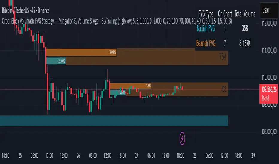
Order Block Volumatic FVG StrategyInspired by: Volumatic Fair Value Gaps —
License: CC BY-NC-SA 4.0 (Creative Commons Attribution–NonCommercial–ShareAlike).
This script is a non-commercial derivative work that credits the original author and keeps the same license.
What this strategy does
This turns BigBeluga’s visual FVG concept into an entry/exit strategy. It scans bullish and bearish FVG boxes, measures how deep price has mitigated into a box (as a percentage), and opens a long/short when your mitigation threshold and filters are satisfied. Risk is managed with a fixed Stop Loss % and a Trailing Stop that activates only after a user-defined profit trigger.
Additions vs. the original indicator
✅ Strategy entries based on % mitigation into FVGs (long/short).
✅ Lower-TF volume split using upticks/downticks; fallback if LTF data is missing (distributes prior bar volume by close’s position in its H–L range) to avoid NaN/0.
✅ Per-FVG total volume filter (min/max) so you can skip weak boxes.
✅ Age filter (min bars since the FVG was created) to avoid fresh/immature boxes.
✅ Bull% / Bear% share filter (the 46%/53% numbers you see inside each FVG).
✅ Optional candle confirmation and cooldown between trades.
✅ Risk management: fixed SL % + Trailing Stop with a profit trigger (doesn’t trail until your trigger is reached).
✅ Pine v6 safety: no unsupported args, no indexof/clamp/when, reverse-index deletes, guards against zero/NaN.
How a trade is decided (logic overview)
Detect FVGs (same rules as the original visual logic).
For each FVG currently intersected by the bar, compute:
Mitigation % (how deep price has entered the box).
Bull%/Bear% split (internal volume share).
Total volume (printed on the box) from LTF aggregation or fallback.
Age (bars) since the box was created.
Apply your filters:
Mitigation ≥ Long/Short threshold.
Volume between your min and max (if enabled).
Age ≥ min bars (if enabled).
Bull% / Bear% within your limits (if enabled).
(Optional) the current candle must be in trade direction (confirm).
If multiple FVGs qualify on the same bar, the strategy uses the most recent one.
Enter long/short (no pyramiding).
Exit with:
Fixed Stop Loss %, and
Trailing Stop that only starts after price reaches your profit trigger %.
Input settings (quick guide)
Mitigation source: close or high/low. Use high/low for intrabar touches; close is stricter.
Mitigation % thresholds: minimal mitigation for Long and Short.
TOTAL Volume filter: skip FVGs with too little/too much total volume (per box).
Bull/Bear share filter: require, e.g., Long only if Bull% ≥ 50; avoid Short when Bull% is high (Short Bull% max).
Age filter (bars): e.g., ≥ 20–30 bars to avoid fresh boxes.
Confirm candle: require candle direction to match the trade.
Cooldown (bars): minimum bars between entries.
Risk:
Stop Loss % (fixed from entry price).
Activate trailing at +% profit (the trigger).
Trailing distance % (the trailing gap once active).
Lower-TF aggregation:
Auto: TF/Divisor → picks 1/3/5m automatically.
Fixed: choose 1/3/5/15m explicitly.
If LTF can’t be fetched, fallback allocates prior bar’s volume by its close position in the bar’s H–L.
Suggested starting presets (you should optimize per market)
Mitigation: 60–80% for both Long/Short.
Bull/Bear share:
Long: Bull% ≥ 50–70, Bear% ≤ 100.
Short: Bull% ≤ 60 (avoid shorting into strong support), Bear% ≥ 0–70 as you prefer.
Age: ≥ 20–30 bars.
Volume: pick a min that filters noise for your symbol/timeframe.
Risk: SL 4–6%, trailing trigger 1–2%, distance 1–2% (crypto example).
Set slippage/fees in Strategy Properties.
Notes, limitations & best practices
Data differences: The LTF split uses request.security_lower_tf. If the exchange/data feed has sparse LTF data, the fallback kicks in (it’s deliberate to avoid NaNs but is a heuristic).
Real-time vs backtest: The current bar can update until close; results on historical bars use closed data. Use “Bar Replay” to understand intrabar effects.
No pyramiding: Only one position at a time. Modify pyramiding in the header if you need scaling.
Assets: For spot/crypto, TradingView “volume” is exchange volume; in some markets it may be tick volume—interpret filters accordingly.
Risk disclosure: Past performance ≠ future results. Use appropriate position sizing and risk controls; this is not financial advice.
Credits
Visual FVG concept and original implementation: BigBeluga.
This derivative strategy adds entry/exit logic, volume/age/share filters, robust LTF handling, and risk management while preserving the original spirit.
License remains CC BY-NC-SA 4.0 (non-commercial, attribution required, share-alike).
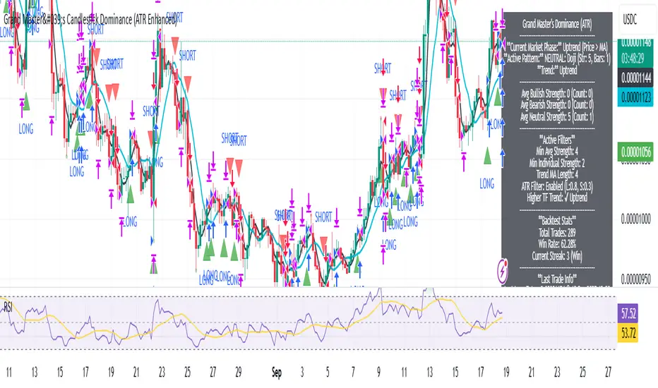
Grand Master's Candlestick Dominance (ATR Enhanced)### Grand Master's Candlestick Dominance (ATR Enhanced)
**Overview**
Unleash the ancient wisdom of Japanese candlestick charting with a modern twist! This comprehensive Pine Script v5 strategy and indicator scans for over 75 classic and advanced candlestick patterns (bullish, bearish, and neutral), assigning dynamic strength scores (1-10) to each for precise signal filtering. Enhanced with Average True Range (ATR) for volatility-aware body size validation, it dominates the markets by combining timeless pattern recognition with robust confirmation layers. Whether used as a backtestable strategy or visual indicator, it empowers traders to spot high-probability reversals, continuations, and indecision setups with surgical accuracy.
Inspired by Steve Nison's *Japanese Candlestick Charting Techniques*, this tool elevates pattern analysis beyond basics—think Hammers, Engulfing patterns, Morning Stars, and rare gems like Abandoned Baby or Concealing Baby Swallow—all consolidated into intelligent arrays for real-time averaging and prioritization.
**Key Features**
- **Extensive Pattern Library**:
- **Bullish (25+ patterns)**: Hammer (8.0), Bullish Engulfing (10.0), Morning Star (7.0), Three White Soldiers (9.0), Dragonfly Doji (8.0), and more (e.g., Rising Three, Unique Three River Bottom).
- **Bearish (25+ patterns)**: Hanging Man (8.0), Bearish Engulfing (10.0), Evening Star (7.0), Three Black Crows (9.0), Gravestone Doji (8.0), and exotics like Upside Gap Two Crows or Stalled Pattern.
- **Neutral/Indecision (34+ patterns)**: Doji variants (Long-Legged, Four Price), Spinning Tops, Harami Crosses, and multi-bar setups like Upside Tasuki Gap or Advancing Block.
Each pattern includes duration tracking (1-5 bars) and ATR-adjusted body/shadow criteria for relevance in volatile conditions.
- **Smart Confirmation Filters** (All Toggleable):
- **Trend Alignment**: 20-period SMA (customizable) ensures entries align with the prevailing trend; optional higher timeframe (e.g., Daily) MA crossover for multi-timeframe confluence.
- **Support/Resistance (S/R)**: Pivot-based levels with 0.01% tolerance to confirm bounces or breaks.
- **Volume Surge**: 20-period volume MA with 1.5x spike multiplier to validate momentum.
- **ATR Body Sizing**: Filters small bodies (<0.3x ATR) and long bodies (>0.8x ATR) for context-aware pattern reliability.
- **Follow-Through**: Ensures post-pattern confirmation via bullish/bearish closes or closes beyond prior bars.
Minimum average strength (default 7.0) and individual pattern thresholds (5.0) prevent weak signals.
- **Entry & Exit Logic**:
- **Long Entry**: Bullish average strength ≥7.0 (outweighing bearish), uptrend, volume spike, near support, follow-through, and HTF alignment.
- **Short Entry**: Mirror for bearish dominance in downtrends near resistance.
- **Exits**: Bearish/neutral shift, or fixed TP (5%) / SL (2%)—pyramiding disabled, 10% equity sizing.
- Backtest range: Jan 1, 2020 – Dec 31, 2025 (editable). Initial capital: $10,000.
- **Interactive Dashboard** (Top-Right Panel):
Real-time insights including:
- Market phase (e.g., "Bullish Phase (Avg Str: 8.2)"), active pattern (e.g., "BULLISH: Bullish Engulfing (Str: 10.0, Bars: 2)"), and trend status.
- Strength breakdowns (Bull/Bear/Neutral counts & averages).
- Filter status (e.g., "Volume: ✔ Spike", "ATR: Enabled (L:0.8, S:0.3)").
- Backtest stats: Total trades, win rate, streak, and last entry/exit details (price & timestamp).
Toggle mode: Strategy (live trades) or Indicator (signals only).
- **Advanced Alerts** (15+ Toggleable Types):
Set up via TradingView's "Any alert() function call" for bar-close triggers:
- Entry/Exit signals with strength & pattern details.
- Strong patterns (≥2 bullish/bearish), neutral indecision, volume spikes.
- S/R breakouts, HTF reversals, high-confidence singles (≥8.0 strength).
- Conflicting signals, MA crossovers, ATR volatility bursts, multi-bar completions.
Example: "STRONG BULLISH PATTERN detected! Strength: 9.5 | Top Pattern: Three White Soldiers | Trend: Up".
**Customization & Usage Tips**
- **Inputs Groups**: Strategy toggles, confirmations, exits, backtest dates, and 15+ alert switches—all intuitively grouped.
- **Optimization**: Tune min strengths for aggressive (lower) or conservative (higher) trading; enable/disable filters to suit your style (e.g., disable S/R for scalping).
- **Best For**: Forex, stocks, crypto on 1H–Daily charts. Test on historical data to refine TP/SL.
- **Limitations**: No external data installs; relies on built-in TA functions. Patterns are probabilistic—combine with your risk management.
Master the candles like a grandmaster. Deploy on TradingView, backtest relentlessly, and let dominance begin! Questions? Drop a comment.
*Version: 1.0 | Updated: September 2025 | Credits: Built on Pine Script v5 with nods to Nison's timeless techniques.*
MS - Çoklu Onay Stratejisi (AL-SAT)"VOLUME, MA50, RSI, DMI, ATR
5 conditions, all turning positive at the same time gives a buy signal; one of them turning negative gives a sell signal. This should be evaluated with weekly data. Not financial advice."

Liquidity Sweep Breakout - LSBLiquidity Sweep Breakout - LSB
A professional session-based breakout system designed for OANDA:USDJPY and other JPY pairs.
Not guesswork, but precision - built on detailed observation of institutional moves to capture clear trade direction daily.
Master the Market’s Daily Bank Flow.
---
Strategy Detail:
I discovered this strategy after carefully studying how Japanese banks influence the forex market during their daily settlement period. Banks are some of the biggest players in the financial world, and when they adjust or settle their accounts in the morning, it often creates a push in the market. From years of observation, I noticed a consistent pattern, once banks finish their settlements, the market usually continues moving in the same direction that was formed right after those actions. This daily banking flow often sets the tone for the entire trading session, especially for JPY pairs like USDJPY.
To capture this move, I built the indicator so that it follows the bank-driven trend with clear rules for entries, stop-loss (SL), and take-profit (TP). The system is designed with professional risk management in mind. By default, it assumes a $10,000 account size, risks only 1% of that balance per trade, and targets a 1:1.5 reward-to-risk ratio. This means for every $100 risked, the potential profit is $150. Such controlled risk makes the system safer and more sustainable for long-term traders. At the same time, users are not limited to this setup, they can adjust the account balance in the settings, and the indicator will automatically recalculate the lot size and risk levels based on their own capital. This ensures the strategy works for small accounts and larger accounts alike.
🌍 Why It Works
Fundamentally driven: Based on **daily Japanese banking settlement flows**.
Session-specific precision: Targets the exact window when USDJPY liquidity reshapes.
Risk-managed: Always calculates lot size based on account and risk preferences.
Automatable: With webhook + MT5 EA, it can be fully hands-free.
---
✅ Recommended
Pair: USDJPY (best observed behavior).
Timeframe: 3-Minute chart.
Platform: TradingView Premium (for webhooks).
Execution: MT5 via EA.
---
🔎 Strategy Concept
The Tokyo Magic Breakout (TMB) is built on years of session observation and the unique daily rhythm of the Japanese banking system.
Every morning between 5:50 AM – 6:10 AM PKT (09:50 – 10:10 JST), Japanese banks perform daily reconciliation and settlement. This often sets the tone for the USDJPY direction of the day.
This strategy isolates that critical moment of liquidity adjustment and waits for a clean breakout confirmation. Instead of chasing noise, it executes only when price action is aligned with the Tokyo market’s hidden flows.
---
🕒 Timing Logic
Session Start: 5:00 AM PKT (Tokyo market open range).
Magic Candle: The 5:54 AM PKT candle is marked as the reference “breakout selector.”
Checkpoints: First confirmation at 6:30 AM PKT, then every 15 minutes until 8:30 AM PKT.
* If price stays inside the magic range → wait.
* If a breakout happens but the candle wick touches the range → wait for the next checkpoint.
* If by 8:30 AM PKT no clean breakout occurs → the day is marked as No Trade Day (NTD).
👉 Recommended timeframe: 3-Minute chart (3M) for precise signals.
---
📈 Trade Execution
Entry: Clean break above/below the magic candle’s range.
Stop-Loss: Opposite side of the Tokyo session high/low.
Take-Profit: Calculated by Reward\:Risk ratio (default 1.5:1).
Lot Size: Auto-calculated based on your risk model:
* Fixed Dollar
* % of Equity
* Conservative (minimum of both).
Visuals include:
✅ Entry/SL/TP lines
✅ Shaded risk (red) and reward (green) zones
✅ Trade labels (Buy/Sell with lot size & levels)
✅ TP/SL hit markers
---
🔔 Alerts & Automation (AutoTMB)
This strategy is fully automation-ready with EA + MT5:
1. Enable alerts in TMB settings.
2. Insert your PineConnector License Key.
3. Configure your risk management preferences.
4. Create a TradingView alert → in the message box simply type:
Pine Script®
{{alert_message}}
and set the EA webhook.
Now, every breakout trade (with exact entry, SL, TP, and lot size) is sent instantly.
👉 On your MT5:
* Install the EA.
* Use the same license key.
* Run it on a VPS or local MT5 terminal.
You now have a hands-free trading system: AutoTMB.

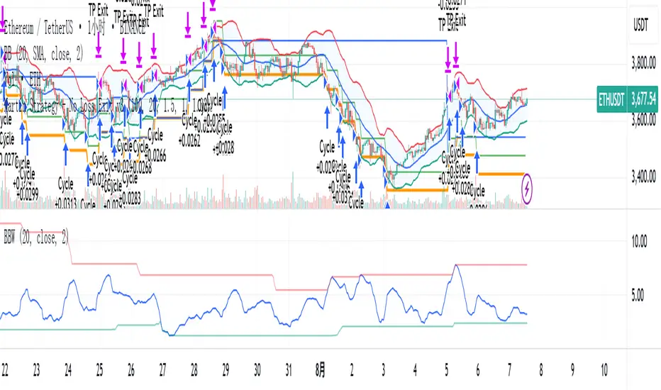
Martin Strategy - No Loss Exit v3Martin Strategy1.0 Martin Strategy1.0 Martin Strategy1.0 Martin Strategy1.0 Martin Strategy1.0 Martin Strategy1.0
PEAD strategy█ OVERVIEW
This strategy trades the classic post-earnings announcement drift (PEAD).
It goes long only when the market gaps up after a positive EPS surprise.
█ LOGIC
1 — Earnings filter — EPS surprise > epsSprThresh %
2 — Gap filter — first regular 5-minute bar gaps ≥ gapThresh % above yesterday’s close
3 — Timing — only the first qualifying gap within one trading day of the earnings bar
4 — Momentum filter — last perfDays trading-day performance is positive
5 — Risk management
• Fixed stop-loss: stopPct % below entry
• Trailing exit: price < Daily EMA( emaLen )
█ INPUTS
• Gap up threshold (%) — 1 (gap size for entry)
• EPS surprise threshold (%) — 5 (min positive surprise)
• Past price performance — 20 (look-back bars for trend check)
• Fixed stop-loss (%) — 8 (hard stop distance)
• Daily EMA length — 30 (trailing exit length)
Note — Back-tests fill on the second 5-minute bar (Pine limitation).
Live trading: enable calc_on_every_tick=true for first-tick entries.
────────────────────────────────────────────
█ 概要(日本語)
本ストラテジーは決算後の PEAD を狙い、
EPS サプライズがプラス かつ 寄付きギャップアップ が発生した銘柄をスイングで買い持ちします。
█ ロジック
1 — 決算フィルター — EPS サプライズ > epsSprThresh %
2 — ギャップフィルター — レギュラー時間最初の 5 分足が前日終値+ gapThresh %以上
3 — タイミング — 決算当日または翌営業日の最初のギャップのみエントリー
4 — モメンタムフィルター — 過去 perfDays 営業日の騰落率がプラス
5 — リスク管理
• 固定ストップ:エントリー − stopPct %
• 利確:終値が日足 EMA( emaLen ) を下抜け
█ 入力パラメータ
• Gap up threshold (%) — 1 (ギャップ条件)
• EPS surprise threshold (%) — 5 (EPS サプライズ最小値)
• Past price performance — 20 (パフォーマンス判定日数)
• Fixed stop-loss (%) — 8 (固定ストップ幅)
• Daily EMA length — 30 (利確用 EMA 期間)
注意 — Pine の仕様上、バックテストでは寄付き 5 分足の次バーで約定します。
実運用で寄付き成行に合わせたい場合は calc_on_every_tick=true を有効にしてください。
────
ご意見や質問があればお気軽にコメントください。
Happy trading!

Sharpe Ratio Forced Selling StrategyThis study introduces the “Sharpe Ratio Forced Selling Strategy”, a quantitative trading model that dynamically manages positions based on the rolling Sharpe Ratio of an asset’s excess returns relative to the risk-free rate. The Sharpe Ratio, first introduced by Sharpe (1966), remains a cornerstone in risk-adjusted performance measurement, capturing the trade-off between return and volatility. In this strategy, entries are triggered when the Sharpe Ratio falls below a specified low threshold (indicating excessive pessimism), and exits occur either when the Sharpe Ratio surpasses a high threshold (indicating optimism or mean reversion) or when a maximum holding period is reached.
The underlying economic intuition stems from institutional behavior. Institutional investors, such as pension funds and mutual funds, are often subject to risk management mandates and performance benchmarking, requiring them to reduce exposure to assets that exhibit deteriorating risk-adjusted returns over rolling periods (Greenwood and Scharfstein, 2013). When risk-adjusted performance improves, institutions may rebalance or liquidate positions to meet regulatory requirements or internal mandates, a behavior that can be proxied effectively through a rising Sharpe Ratio.
By systematically monitoring the Sharpe Ratio, the strategy anticipates when “forced selling” pressure is likely to abate, allowing for opportunistic entries into assets priced below fundamental value. Exits are equally mechanized, either triggered by Sharpe Ratio improvements or by a strict time-based constraint, acknowledging that institutional rebalancing and window-dressing activities are often time-bound (Coval and Stafford, 2007).
The Sharpe Ratio is particularly suitable for this framework due to its ability to standardize excess returns per unit of risk, ensuring comparability across timeframes and asset classes (Sharpe, 1994). Furthermore, adjusting returns by a dynamically updating short-term risk-free rate (e.g., US 3-Month T-Bills from FRED) ensures that macroeconomic conditions, such as shifting interest rates, are accurately incorporated into the risk assessment.
While the Sharpe Ratio is an efficient and widely recognized measure, the strategy could be enhanced by incorporating alternative or complementary risk metrics:
• Sortino Ratio: Unlike the Sharpe Ratio, the Sortino Ratio penalizes only downside volatility (Sortino and van der Meer, 1991). This would refine entries and exits to distinguish between “good” and “bad” volatility.
• Maximum Drawdown Constraints: Integrating a moving window maximum drawdown filter could prevent entries during persistent downtrends not captured by volatility alone.
• Conditional Value at Risk (CVaR): A measure of expected shortfall beyond the Value at Risk, CVaR could further constrain entry conditions by accounting for tail risk in extreme environments (Rockafellar and Uryasev, 2000).
• Dynamic Thresholds: Instead of static Sharpe thresholds, one could implement dynamic bands based on the historical distribution of the Sharpe Ratio, adjusting for volatility clustering effects (Cont, 2001).
Each of these risk parameters could be incorporated into the current script as additional input controls, further tailoring the model to different market regimes or investor risk appetites.
References
• Cont, R. (2001) ‘Empirical properties of asset returns: stylized facts and statistical issues’, Quantitative Finance, 1(2), pp. 223-236.
• Coval, J.D. and Stafford, E. (2007) ‘Asset Fire Sales (and Purchases) in Equity Markets’, Journal of Financial Economics, 86(2), pp. 479-512.
• Greenwood, R. and Scharfstein, D. (2013) ‘The Growth of Finance’, Journal of Economic Perspectives, 27(2), pp. 3-28.
• Rockafellar, R.T. and Uryasev, S. (2000) ‘Optimization of Conditional Value-at-Risk’, Journal of Risk, 2(3), pp. 21-41.
• Sharpe, W.F. (1966) ‘Mutual Fund Performance’, Journal of Business, 39(1), pp. 119-138.
• Sharpe, W.F. (1994) ‘The Sharpe Ratio’, Journal of Portfolio Management, 21(1), pp. 49-58.
• Sortino, F.A. and van der Meer, R. (1991) ‘Downside Risk’, Journal of Portfolio Management, 17(4), pp. 27-31.

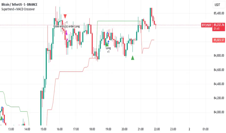
Supertrend + MACD CrossoverKey Elements of the Template:
Supertrend Settings:
supertrendFactor: Adjustable to control the sensitivity of the Supertrend.
supertrendATRLength: ATR length used for Supertrend calculation.
MACD Settings:
macdFastLength, macdSlowLength, macdSignalSmoothing: These settings allow you to fine-tune the MACD for better results.
Risk Management:
Stop-Loss: The stop-loss is based on the ATR (Average True Range), a volatility-based indicator.
Take-Profit: The take-profit is based on the risk-reward ratio (set to 3x by default).
Both stop-loss and take-profit are dynamic, based on ATR, which adjusts according to market volatility.
Buy and Sell Signals:
Buy Signal: Supertrend is bullish, and MACD line crosses above the Signal line.
Sell Signal: Supertrend is bearish, and MACD line crosses below the Signal line.
Visual Elements:
The Supertrend line is plotted in green (bullish) and red (bearish).
Buy and Sell signals are shown with green and red triangles on the chart.
Next Steps for Optimization:
Backtesting:
Run backtests on BTC in the 5-minute timeframe and adjust parameters (Supertrend factor, MACD settings, risk-reward ratio) to find the optimal configuration for the 60% win ratio.
Fine-Tuning Parameters:
Adjust supertrendFactor and macdFastLength to find more optimal values based on BTC's market behavior.
Tweak the risk-reward ratio to maximize profitability while maintaining a good win ratio.
Evaluate Market Conditions:
The performance of the strategy can vary based on market volatility. It may be helpful to evaluate performance in different market conditions or pair it with a filter like RSI or volume.
Let me know if you'd like further tweaks or explanations!
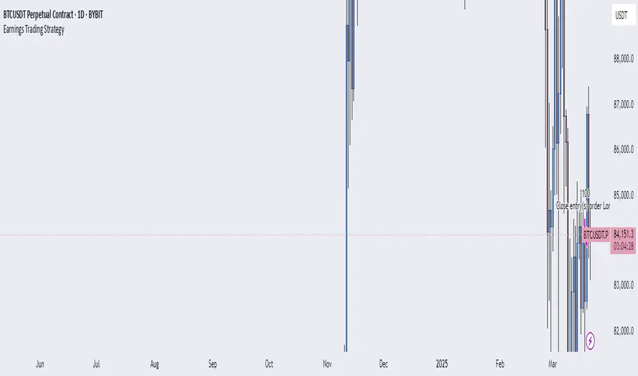
Earnings Trading StrategyThe Earnings Trade Strategy automates the process of entering and exiting trades based on earnings announcements for Apple (AAPL). It allows users to take a position—either long (buy) or short (sell short)—on the trading day before an earnings announcement and close that position on the trading day after the announcement. By leveraging TradingView’s Paper Trading environment, the strategy enables users to simulate trades and collect performance data over a 6-month period in a risk-free setting.
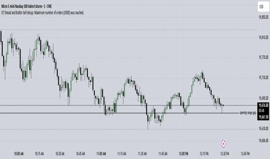
ICT Bread and Butter Sell-SetupICT Bread and Butter Sell-Setup – TradingView Strategy
Overview:
The ICT Bread and Butter Sell-Setup is an intraday trading strategy designed to capitalize on bearish market conditions. It follows institutional order flow and exploits liquidity patterns within key trading sessions—London, New York, and Asia—to identify high-probability short entries.
Key Components of the Strategy:
🔹 London Open Setup (2:00 AM – 8:20 AM NY Time)
The London session typically sets the initial directional move of the day.
A short-term high often forms before a downward push, establishing the daily high.
🔹 New York Open Kill Zone (8:20 AM – 10:00 AM NY Time)
The New York Judas Swing (a temporary rally above London’s high) creates an opportunity for short entries.
Traders fade this move, anticipating a sell-off targeting liquidity below previous lows.
🔹 London Close Buy Setup (10:30 AM – 1:00 PM NY Time)
If price reaches a higher timeframe discount array, a retracement higher is expected.
A bullish order block or failure swing signals a possible reversal.
The risk is set just below the day’s low, targeting a 20-30% retracement of the daily range.
🔹 Asia Open Sell Setup (7:00 PM – 2:00 AM NY Time)
If institutional order flow remains bearish, a short entry is taken around the 0-GMT Open.
Expect a 15-20 pip decline as the Asian range forms.
Strategy Rules:
📉 Short Entry Conditions:
✅ New York Judas Swing occurs (price moves above London’s high before reversing).
✅ Short entry is triggered when price closes below the open.
✅ Stop-loss is set 10 pips above the session high.
✅ Take-profit targets liquidity zones on higher timeframes.
📈 Long Entry (London Close Reversal):
✅ Price reaches a higher timeframe discount array between 10:30 AM – 1:00 PM NY Time.
✅ A bullish order block confirms the reversal.
✅ Stop-loss is set 10 pips below the day’s low.
✅ Take-profit targets 20-30% of the daily range retracement.
📉 Asia Open Sell Entry:
✅ Price trades slightly above the 0-GMT Open.
✅ Short entry is taken at resistance, targeting a quick 15-20 pip move.
Why Use This Strategy?
🚀 Institutional Order Flow Tracking – Aligns with smart money concepts.
📊 Precise Session Timing – Uses market structure across London, New York, and Asia.
🎯 High-Probability Entries – Focuses on liquidity grabs and engineered stop hunts.
📉 Optimized Risk Management – Defined stop-loss and take-profit levels.
This strategy is ideal for traders looking to trade with institutions, fade liquidity grabs, and capture high-probability short setups during the trading day. 📉🔥
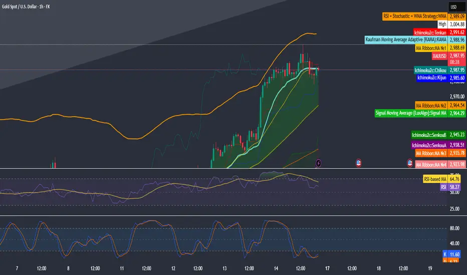
RSI + Stochastic + WMA StrategyThis script is designed for TradingView and serves as a trading strategy (not just a visual indicator). It's intended for backtesting, strategy optimization, or live trading signal generation using a combination of popular technical indicators.
📊 Indicators Used in the Strategy:
Indicator Description
RSI (Relative Strength Index) Measures momentum; identifies overbought (>70) or oversold (<30) conditions.
Stochastic Oscillator (%K & %D) Detects momentum reversal points via crossovers. Useful for timing entries.
WMA (Weighted Moving Average) Identifies the trend direction (used as a trend filter).
📈 Trading Logic / Strategy Rules:
📌 Long Entry Condition (Buy Signal):
All 3 conditions must be true:
RSI is Oversold → RSI < 30
Stochastic Crossover Upward → %K crosses above %D
Price is above WMA → Confirms uptrend direction
👉 Interpretation: Market was oversold, momentum is turning up, and price confirms uptrend — bullish entry.
📌 Short Entry Condition (Sell Signal):
All 3 conditions must be true:
RSI is Overbought → RSI > 70
Stochastic Crossover Downward → %K crosses below %D
Price is below WMA → Confirms downtrend direction
👉 Interpretation: Market is overbought, momentum is turning down, and price confirms downtrend — bearish entry.
🔄 Strategy Execution (Backtesting Logic):
The script uses:
pinescript
Copy
Edit
strategy.entry("LONG", strategy.long)
strategy.entry("SHORT", strategy.short)
These are Pine Script functions to place buy and sell orders automatically when the above conditions are met. This allows you to:
Backtest the strategy
Measure win/loss ratio, drawdown, and profitability
Optimize indicator settings using TradingView Strategy Tester
📊 Visual Aids (Charts):
Plots WMA Line: Orange line for trend direction
Overbought/Oversold Zones: Horizontal lines at 70 (red) and 30 (green) for RSI visualization
⚡ Strategy Type Summary:
Category Setting
Strategy Type Momentum Reversal + Trend Filter
Timeframe Flexible (Works best on 1H, 4H, Daily)
Trading Style Swing/Intraday
Risk Profile Medium to High (due to momentum triggers)
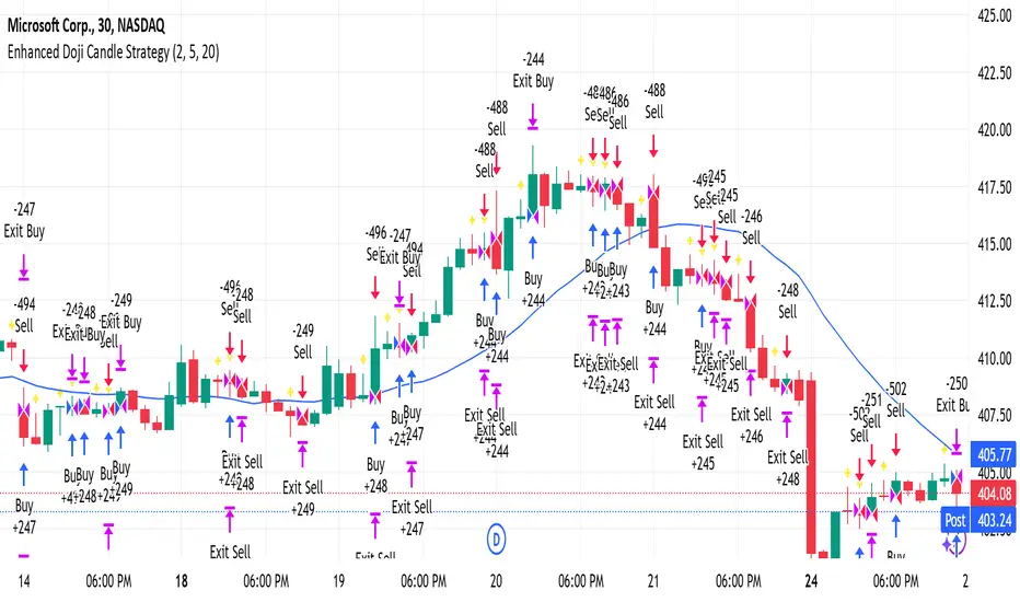
Uses Leverage Possible (adjust risk accordingly)
Enhanced Doji Candle StrategyYour trading strategy is a Doji Candlestick Reversal Strategy designed to identify potential market reversals using Doji candlestick patterns. These candles indicate indecision in the market, and when detected, your strategy uses a Simple Moving Average (SMA) with a short period of 20 to confirm the overall market trend. If the price is above the SMA, the trend is considered bullish; if it's below, the trend is bearish.
Once a Doji is detected, the strategy waits for one or two consecutive confirmation candles that align with the market trend. For a bullish confirmation, the candles must close higher than their opening price without significant bottom wicks. Conversely, for a bearish confirmation, the candles must close lower without noticeable top wicks. When these conditions are met, a trade is entered at the market price.
The risk management aspect of your strategy is clearly defined. A stop loss is automatically placed at the nearest recent swing high or low, with a tighter distance of 5 pips to allow for more trading opportunities. A take-profit level is set using a 2:1 reward-to-risk ratio, meaning the potential reward is twice the size of the risk on each trade.
Additionally, the strategy incorporates an early exit mechanism. If a reversal Doji forms in the opposite direction of your trade, the position is closed immediately to minimize losses. This strategy has been optimized to increase trade frequency by loosening the strictness of Doji detection and confirmation conditions while still maintaining sound risk management principles.
The strategy is coded in Pine Script for use on TradingView and uses built-in indicators like the SMA for trend detection. You also have flexible parameters to adjust risk levels, take-profit targets, and stop-loss placements, allowing you to tailor the strategy to different market conditions.
SPY/TLT Strategy█ STRATEGY OVERVIEW
The "SPY/TLT Strategy" is a trend-following crossover strategy designed to trade the relationship between TLT and its Simple Moving Average (SMA). The default configuration uses TLT (iShares 20+ Year Treasury Bond ETF) with a 20-period SMA, entering long positions on bullish crossovers and exiting on bearish crossunders. **This strategy is NOT optimized and performs best in trending markets.**
█ KEY FEATURES
SMA Crossover System: Uses price/SMA relationship for signal generation (Default: 20-period)
Dynamic Time Window: Configurable backtesting period (Default: 2014-2099)
Equity-Based Position Sizing: Default 100% equity allocation per trade
Real-Time Visual Feedback: Price/SMA plot with trend-state background coloring
Event-Driven Execution: Processes orders at bar close for accurate backtesting
█ SIGNAL GENERATION
1. LONG ENTRY CONDITION
TLT closing price crosses ABOVE SMA
Occurs within specified time window
Generates market order at next bar open
2. EXIT CONDITION
TLT closing price crosses BELOW SMA
Closes all open positions immediately
█ ADDITIONAL SETTINGS
SMA Period: Simple Moving Average length (Default: 20)
Start Time and End Time: The time window for trade execution (Default: 1 Jan 2014 - 1 Jan 2099)
Security Symbol: Ticker for analysis (Default: TLT)
█ PERFORMANCE OVERVIEW
Ideal Market Conditions: Strong trending environments
Potential Drawbacks: Whipsaws in range-bound markets
Backtesting results should be analyzed to optimize the MA Period and EMA Filter settings for specific instruments

Fibonacci Levels Strategy with High/Low Criteria-AYNETThis code represents a TradingView strategy that uses Fibonacci levels in conjunction with high/low price criteria over specified lookback periods to determine buy (long) and sell (short) conditions. Below is an explanation of each main part of the code:
Explanation of Key Sections
User Inputs for Higher Time Frame and Candle Settings
Users can select a higher time frame (timeframe) for analysis and specify whether to use the "Current" or "Last" higher time frame (HTF) candle for calculating Fibonacci levels.
The currentlast setting allows flexibility between using real-time or the most recent closed higher time frame candle.
Lookback Periods for High/Low Criteria
Two lookback periods, lowestLookback and highestLookback, allow users to set the number of bars to consider when finding the lowest and highest prices, respectively.
This determines the criteria for entering trades based on how recent highs or lows compare to current prices.
Fibonacci Levels Configuration
Fibonacci levels (0%, 23.6%, 38.2%, 50%, 61.8%, 78.6%, and 100%) are configurable. These are used to calculate price levels between the high and low of the higher time frame candle.
Each level represents a retracement or extension relative to the high/low range of the HTF candle, providing important price levels for decision-making.
HTF Candle Calculation
HTF candle data is calculated based on the higher time frame selected by the user, using the newbar check to reset htfhigh, htflow, and htfopen values.
The values are updated with each new HTF bar or as prices move within the same HTF bar to track the highest high and lowest low accurately.
Set Fibonacci Levels Array
Using the calculated HTF candle's high, low, and open, the Fibonacci levels are computed by interpolating these values according to the user-defined Fibonacci levels.
A fibLevels array stores these computed values.
Plotting Fibonacci Levels
Each Fibonacci level is plotted on the chart with a different color, providing visual indicators for potential support/resistance levels.
High/Low Price Criteria Calculation
The lowest and highest prices over the specified lookback periods (lowestLookback and highestLookback) are calculated and plotted on the chart. These serve as dynamic levels to trigger long or short entries.
Trade Signal Conditions
longCondition: A long (buy) signal is generated when the price crosses above both the lowest price criteria and the 50% Fibonacci level.
shortCondition: A short (sell) signal is generated when the price crosses below both the highest price criteria and the 50% Fibonacci level.
Executing Trades
Based on the longCondition and shortCondition, trades are entered with the strategy.entry() function, using the labels "Long" and "Short" for tracking on the chart.
Strategy Use
This strategy allows traders to utilize Fibonacci retracement levels and recent highs/lows to identify trend continuation or reversal points, potentially providing entry points aligned with larger market structure. Adjusting the lowestLookback and highestLookback along with Fibonacci levels enables a customizable approach to suit different trading styles and market conditions.
