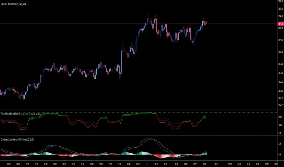
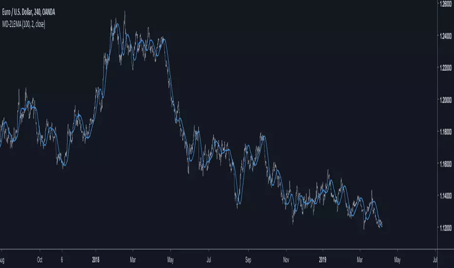
Local Model Kalman Market ModeIntroduction
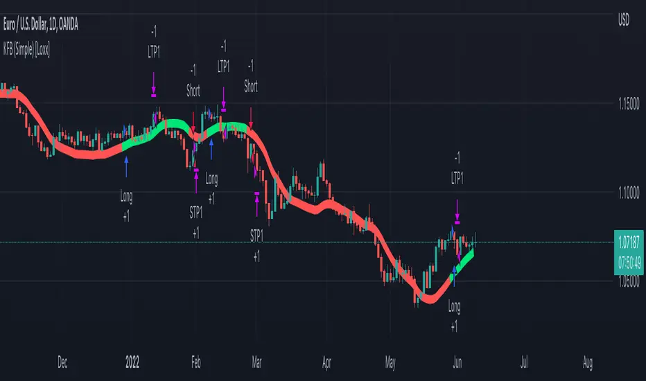
Heyo guys, I made a new (repainting) indicator called Local Model Kalman Market Mode.
I created it, because I wanted a reliable market mode filter for a potential mean-reversion strategy (e. g. BB Scalping).
On the screenshot you can see an example of how to use it in a BB strategy.
E.g. you would enter long when you have bullish divergence, price is under lower BB, price is under PoC and this indicator here shows range-bound market phase.
You would exit long on cross of the middle band.
Description
The indicator attempts to model the underlying market using different local models (i.e., trending, range-bound, and choppy) and combines them using the T3 Six Pole Kalman Filter to generate an overall estimate of the market.
The Fisher Transform is applied on the price to reach a Gaussian distribution, which increases the accuracy of the indicator itself.
The script first defines state variables for each local model, which include trend direction, trend strength, upper and lower bounds of the range, volatility of the range, level of choppiness, and strength of noise.
Then, likelihood functions are defined for each local model based on the state variables.
Next, the script calculates weights for each local model based on their likelihoods and uses them to calculate state variables for the overall estimate.
Finally, the script combines the state variables using the T3 Six Pole Kalman Filter to generate the overall estimate of the market, which is plotted in blue.
Fundamental Knowledge
To understand the explanation of the indicator and the script, there are a few fundamental concepts that you need to know:
Market: A market is a place where buyers and sellers come together to exchange goods or services.
In the context of trading, the market refers to the exchange where financial instruments such as stocks, currencies, and commodities are bought and sold.
Local models: Local models are statistical models that attempt to capture the characteristics of a particular market regime.
For example, a trending market may have different characteristics than a range-bound market or a choppy market.
The indicator uses different local models to capture the different market regimes.
Trend direction and strength: The trend direction refers to the direction in which the market is moving, either up or down.
The trend strength refers to the magnitude of the trend and how likely it is to continue.
Range-bound market: A range-bound market is a market where prices are trading within a specific range, with a clear upper and lower bound.
Choppiness: Choppiness refers to the degree of irregularity in price movements, often seen in sideways or range-bound markets.
Volatility: Volatility refers to the degree of variation in the price of an asset over time. High volatility implies larger price swings, while low volatility implies smaller price swings.
Kalman filter: A Kalman filter is a mathematical algorithm used to estimate an unknown variable from a series of noisy measurements.
In the context of the indicator, the Kalman filter is used to generate an overall estimate of the market by combining the local models.
T3 Six Pole Kalman Filter: The T3 Six Pole Kalman Filter is a specific type of Kalman filter that is used to smooth and filter time-series data, such as the price data of a financial instrument.
Fisher Transform: The Fisher Transform is a mathematical formula used to transform any probability distribution into a Gaussian normal distribution. It is commonly used in technical analysis to transform non-Gaussian indicators into ones that are more suitable for statistical analysis.
By understanding these fundamental concepts, you should have a basic understanding of how the indicator works and how it generates an overall estimate of the market.
Usage
You can use this indicator on every timeframe.
Users can customize the parameters of the T3 Six Pole Kalman Filter (T3 length, alpha, beta, gamma, and delta) using input functions.
Try out different parameter combinations and use the one you like most.
Thank you for checking this out. Leave me a comment or boost the script, when you wanna support me! 👌
--
Credits to:
▪@HPotter - Fisher Transform
▪@loxx - T3
▪ChatGPT - Helped me to make the research for this indicator and helped to build the core algorithm.
Kalman

Kalman Filter [by Hajixde]A simple form of recursive filtering using an adjustable gain and a memory length.
The filter predicts the next sample based on the previous values and the calculated error.
HMA-Kahlman Trend & Trendlines (v.2)This is an upgrade to the HMA-Kahlman Trend & Trendlines script ().
This version gives more flexibility because you can play around with 2 parameters to Kalman function (Sharpness and K (aka. step size)).
Kalman Gain Parameter MechanicsFrequently asked question is to explain how Gain parameter works in kalman funtion. This script serves as a visual representation of Gain parameter of Kalman function used in HMA-Kalman & Trendlines script. (The function creator's name was misspeled in that script as Kahlman)
To see better results set your Chart's timeframe to Daily.

STD/Clutter Filtered, One-Sided, N-Sinc-Kernel, EFIR Filt [Loxx]STD/Clutter Filtered, One-Sided, N-Sinc-Kernel, EFIR Filt is a normalized Cardinal Sine Filter Kernel Weighted Fir Filter that uses Ehler's FIR filter calculation instead of the general FIR filter calculation. This indicator has Kalman Velocity lag reduction, a standard deviation filter, a clutter filter, and a kernel noise filter. When calculating the Kernels, the both sides are calculated, then smoothed, then sliced to just the Right side of the Kernel weights. Lastly, blackman windowing is used for our purposes here. You can read about blackman windowing here:
Blackman window
Advantages of Blackman Window over Hamming Window Method for designing FIR Filter
The Kernel amplitudes are shown below with their corresponding values in yellow:
This indicator is intended to be used with Heikin-Ashi source inputs, specially HAB Median. You can read about this here:
Moving Average Filters Add-on w/ Expanded Source Types
What is a Finite Impulse Response Filter?
In signal processing, a finite impulse response (FIR) filter is a filter whose impulse response (or response to any finite length input) is of finite duration, because it settles to zero in finite time. This is in contrast to infinite impulse response (IIR) filters, which may have internal feedback and may continue to respond indefinitely (usually decaying).
The impulse response (that is, the output in response to a Kronecker delta input) of an Nth-order discrete-time FIR filter lasts exactly {\displaystyle N+1}N+1 samples (from first nonzero element through last nonzero element) before it then settles to zero.
FIR filters can be discrete-time or continuous-time, and digital or analog.
A FIR filter is (similar to, or) just a weighted moving average filter, where (unlike a typical equally weighted moving average filter) the weights of each delay tap are not constrained to be identical or even of the same sign. By changing various values in the array of weights (the impulse response, or time shifted and sampled version of the same), the frequency response of a FIR filter can be completely changed.
An FIR filter simply CONVOLVES the input time series (price data) with its IMPULSE RESPONSE. The impulse response is just a set of weights (or "coefficients") that multiply each data point. Then you just add up all the products and divide by the sum of the weights and that is it; e.g., for a 10-bar SMA you just add up 10 bars of price data (each multiplied by 1) and divide by 10. For a weighted-MA you add up the product of the price data with triangular-number weights and divide by the total weight.
Ultra Low Lag Moving Average's weights are designed to have MAXIMUM possible smoothing and MINIMUM possible lag compatible with as-flat-as-possible phase response.
Ehlers FIR Filter
Ehlers Filter (EF) was authored, not surprisingly, by John Ehlers. Read all about them here: Ehlers Filters
What is Normalized Cardinal Sine?
The sinc function sinc (x), also called the "sampling function," is a function that arises frequently in signal processing and the theory of Fourier transforms.
In mathematics, the historical unnormalized sinc function is defined for x ≠ 0 by
sinc x = sinx / x
In digital signal processing and information theory, the normalized sinc function is commonly defined for x ≠ 0 by
sinc x = sin(pi * x) / (pi * x)
What is a Clutter Filter?
For our purposes here, this is a filter that compares the slope of the trading filter output to a threshold to determine whether to shift trends. If the slope is up but the slope doesn't exceed the threshold, then the color is gray and this indicates a chop zone. If the slope is down but the slope doesn't exceed the threshold, then the color is gray and this indicates a chop zone. Alternatively if either up or down slope exceeds the threshold then the trend turns green for up and red for down. Fro demonstration purposes, an EMA is used as the moving average. This acts to reduce the noise in the signal.
What is a Dual Element Lag Reducer?
Modifies an array of coefficients to reduce lag by the Lag Reduction Factor uses a generic version of a Kalman velocity component to accomplish this lag reduction is achieved by applying the following to the array:
2 * coeff - coeff
The response time vs noise battle still holds true, high lag reduction means more noise is present in your data! Please note that the beginning coefficients which the modifying matrix cannot be applied to (coef whose indecies are < LagReductionFactor) are simply multiplied by two for additional smoothing .
Included
Bar coloring
Loxx's Expanded Source Types
Signals
Alerts

Pips-Stepped, R-squared Adaptive T3 [Loxx]Pips-Stepped, R-squared Adaptive T3 is a a T3 moving average with optional adaptivity, trend following, and pip-stepping. This indicator also uses optional flat coloring to determine chops zones. This indicator is R-squared adaptive. This is also an experimental indicator.
What is the T3 moving average?
Better Moving Averages Tim Tillson
November 1, 1998
Tim Tillson is a software project manager at Hewlett-Packard, with degrees in Mathematics and Computer Science. He has privately traded options and equities for 15 years.
Introduction
"Digital filtering includes the process of smoothing, predicting, differentiating, integrating, separation of signals, and removal of noise from a signal. Thus many people who do such things are actually using digital filters without realizing that they are; being unacquainted with the theory, they neither understand what they have done nor the possibilities of what they might have done."
This quote from R. W. Hamming applies to the vast majority of indicators in technical analysis . Moving averages, be they simple, weighted, or exponential, are lowpass filters; low frequency components in the signal pass through with little attenuation, while high frequencies are severely reduced.
"Oscillator" type indicators (such as MACD , Momentum, Relative Strength Index ) are another type of digital filter called a differentiator.
Tushar Chande has observed that many popular oscillators are highly correlated, which is sensible because they are trying to measure the rate of change of the underlying time series, i.e., are trying to be the first and second derivatives we all learned about in Calculus.
We use moving averages (lowpass filters) in technical analysis to remove the random noise from a time series, to discern the underlying trend or to determine prices at which we will take action. A perfect moving average would have two attributes:
It would be smooth, not sensitive to random noise in the underlying time series. Another way of saying this is that its derivative would not spuriously alternate between positive and negative values.
It would not lag behind the time series it is computed from. Lag, of course, produces late buy or sell signals that kill profits.
The only way one can compute a perfect moving average is to have knowledge of the future, and if we had that, we would buy one lottery ticket a week rather than trade!
Having said this, we can still improve on the conventional simple, weighted, or exponential moving averages. Here's how:
Two Interesting Moving Averages
We will examine two benchmark moving averages based on Linear Regression analysis.
In both cases, a Linear Regression line of length n is fitted to price data.
I call the first moving average ILRS, which stands for Integral of Linear Regression Slope. One simply integrates the slope of a linear regression line as it is successively fitted in a moving window of length n across the data, with the constant of integration being a simple moving average of the first n points. Put another way, the derivative of ILRS is the linear regression slope. Note that ILRS is not the same as a SMA ( simple moving average ) of length n, which is actually the midpoint of the linear regression line as it moves across the data.
We can measure the lag of moving averages with respect to a linear trend by computing how they behave when the input is a line with unit slope. Both SMA (n) and ILRS(n) have lag of n/2, but ILRS is much smoother than SMA .
Our second benchmark moving average is well known, called EPMA or End Point Moving Average. It is the endpoint of the linear regression line of length n as it is fitted across the data. EPMA hugs the data more closely than a simple or exponential moving average of the same length. The price we pay for this is that it is much noisier (less smooth) than ILRS, and it also has the annoying property that it overshoots the data when linear trends are present.
However, EPMA has a lag of 0 with respect to linear input! This makes sense because a linear regression line will fit linear input perfectly, and the endpoint of the LR line will be on the input line.
These two moving averages frame the tradeoffs that we are facing. On one extreme we have ILRS, which is very smooth and has considerable phase lag. EPMA has 0 phase lag, but is too noisy and overshoots. We would like to construct a better moving average which is as smooth as ILRS, but runs closer to where EPMA lies, without the overshoot.
A easy way to attempt this is to split the difference, i.e. use (ILRS(n)+EPMA(n))/2. This will give us a moving average (call it IE /2) which runs in between the two, has phase lag of n/4 but still inherits considerable noise from EPMA. IE /2 is inspirational, however. Can we build something that is comparable, but smoother? Figure 1 shows ILRS, EPMA, and IE /2.
Filter Techniques
Any thoughtful student of filter theory (or resolute experimenter) will have noticed that you can improve the smoothness of a filter by running it through itself multiple times, at the cost of increasing phase lag.
There is a complementary technique (called twicing by J.W. Tukey) which can be used to improve phase lag. If L stands for the operation of running data through a low pass filter, then twicing can be described by:
L' = L(time series) + L(time series - L(time series))
That is, we add a moving average of the difference between the input and the moving average to the moving average. This is algebraically equivalent to:
2L-L(L)
This is the Double Exponential Moving Average or DEMA , popularized by Patrick Mulloy in TASAC (January/February 1994).
In our taxonomy, DEMA has some phase lag (although it exponentially approaches 0) and is somewhat noisy, comparable to IE /2 indicator.
We will use these two techniques to construct our better moving average, after we explore the first one a little more closely.
Fixing Overshoot
An n-day EMA has smoothing constant alpha=2/(n+1) and a lag of (n-1)/2.
Thus EMA (3) has lag 1, and EMA (11) has lag 5. Figure 2 shows that, if I am willing to incur 5 days of lag, I get a smoother moving average if I run EMA (3) through itself 5 times than if I just take EMA (11) once.
This suggests that if EPMA and DEMA have 0 or low lag, why not run fast versions (eg DEMA (3)) through themselves many times to achieve a smooth result? The problem is that multiple runs though these filters increase their tendency to overshoot the data, giving an unusable result. This is because the amplitude response of DEMA and EPMA is greater than 1 at certain frequencies, giving a gain of much greater than 1 at these frequencies when run though themselves multiple times. Figure 3 shows DEMA (7) and EPMA(7) run through themselves 3 times. DEMA^3 has serious overshoot, and EPMA^3 is terrible.
The solution to the overshoot problem is to recall what we are doing with twicing:
DEMA (n) = EMA (n) + EMA (time series - EMA (n))
The second term is adding, in effect, a smooth version of the derivative to the EMA to achieve DEMA . The derivative term determines how hot the moving average's response to linear trends will be. We need to simply turn down the volume to achieve our basic building block:
EMA (n) + EMA (time series - EMA (n))*.7;
This is algebraically the same as:
EMA (n)*1.7-EMA( EMA (n))*.7;
I have chosen .7 as my volume factor, but the general formula (which I call "Generalized Dema") is:
GD (n,v) = EMA (n)*(1+v)-EMA( EMA (n))*v,
Where v ranges between 0 and 1. When v=0, GD is just an EMA , and when v=1, GD is DEMA . In between, GD is a cooler DEMA . By using a value for v less than 1 (I like .7), we cure the multiple DEMA overshoot problem, at the cost of accepting some additional phase delay. Now we can run GD through itself multiple times to define a new, smoother moving average T3 that does not overshoot the data:
T3(n) = GD ( GD ( GD (n)))
In filter theory parlance, T3 is a six-pole non-linear Kalman filter. Kalman filters are ones which use the error (in this case (time series - EMA (n)) to correct themselves. In Technical Analysis , these are called Adaptive Moving Averages; they track the time series more aggressively when it is making large moves.
What is R-squared Adaptive?
One tool available in forecasting the trendiness of the breakout is the coefficient of determination (R-squared), a statistical measurement.
The R-squared indicates linear strength between the security's price (the Y - axis) and time (the X - axis). The R-squared is the percentage of squared error that the linear regression can eliminate if it were used as the predictor instead of the mean value. If the R-squared were 0.99, then the linear regression would eliminate 99% of the error for prediction versus predicting closing prices using a simple moving average.
R-squared is used here to derive a T3 factor used to modify price before passing price through a six-pole non-linear Kalman filter.
Included:
Bar coloring
Signals
Alerts
Flat coloring
Kalman Filter Backtest (Simple) [Loxx]Simple backtest for Kalman Filter found here:
What this backtest includes:
-Longs and shorts
-Customization of inputs for Kalman Filter calculation
-Take profit 1 (TP1), and Stop-loss (SL), calculated using standard RMA-smoothed ATR
-Activation of TP1 after entry candle closes
Happy trading!
Kalman Filter [Loxx]Kalman filter is a recursive algorithm that has been invented in the 1960s to track a moving target, remove any noisy measurements of its position and predict its future position. In finance, KF has been used by the asset management industry for various purposes. KF is an optimal choice in many cases and do at least better than a moving average smoothing.
A port of Kalman filter - indicator for MetaTrader 4
Added color change based on whether velocity is over/under 0
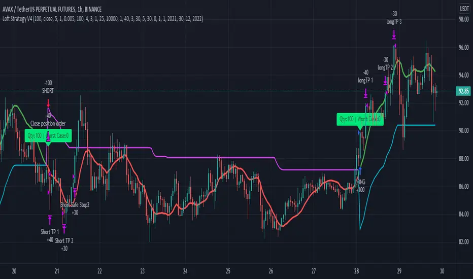
Loft Strategy V4This strategy is an advanced version of the Loft Strategy V1, I shared earlier. (Loft Strategy V1 consists of a kalman filter (by alexgrover ) and a "stop and reverse" line which is following and the kalman filter. If the price goes in the same direction as the position side, the "stop and reverse" line approaches the kalman filter as set on the "Approach Decrease Step" parameter.)
In addition to the previous version, it includes a martingale like deviation and multiple take-profit.
Here it is some parameters definitions of the strategy:
Kalman Filter: The higher this parameter, the faster and more aggressive the filter. Otherwise the filter goes very smoothly
Beginning Approach: First approximation as a percentage of stop-n-reverse line
Final Approach: Minimum approximation of stop-n-reverse line
Approach Decrease Step: If the price moves in the same direction as the strategy, the approach percentage is reduced by this parameter. Otherwise nothing do
Base Order Quantity: Initial capital of position
Max Safe Order Attempt: This parameter determines the maximum number of times the strategy will raise the bet after losing in a row.
Safe Order Deviation: if the last trade is loss, multiply the bet by this parameter (aka. martingale factor)
Profit Deviation: if last trade in loss, multiply the take-profit points
Max Order Quantity: Maximum capital allowed for a position
TP1, TP2, TP3 : Take profit spots in percentage
QT1, QT2, QT3: Amount of take-profit spots
Stop Loss: Maximum stop loss allowed for a trade
Long Entry, Short Entry: Only long side, only short side or both side
Safe Stop After TP2: If the price reaches the TP2 point, move the stop-loss point to the entry price.
Safe Stop After TP1: If the price reaches TP1, move the stop-loss point to the stop-n-reverse line.
Loft Strategy V1This strategy consists of a kalman filter (by alexgrover ) and a "stop and reverse" line which is following the kalman filter.
If the price goes in the same direction as the position side, the "stop and reverse" line approaches the kalman filter as set on the "Approach Decrease Step" parameter.

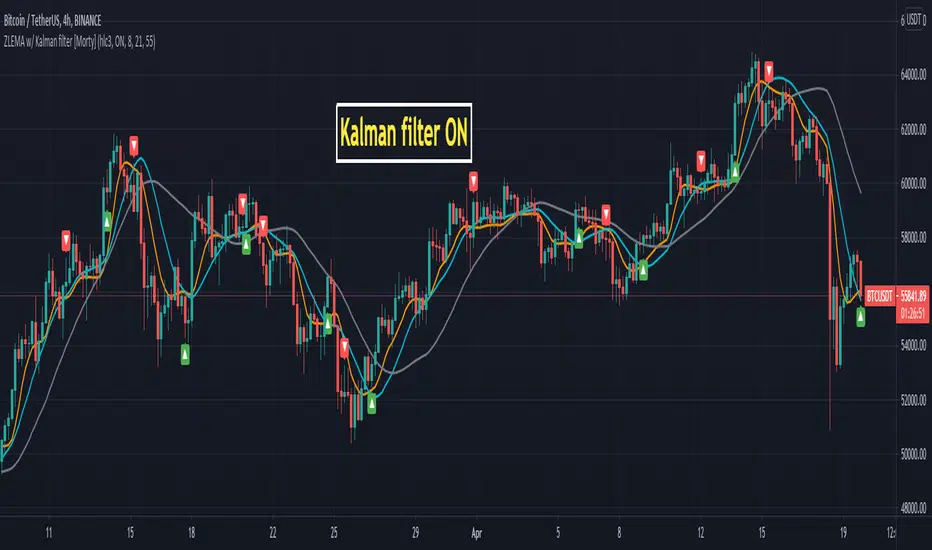
ZLEMA Zero lag EMA with Kalman filter [Morty]This indicator plot 3 Kalman filter zero lag EMA lines. It has less lag and is also smoother than the original EMA.
It also has an option to show the crossover of two EMAs.

OneGreenCandle Kalman - RSIKalman filter on multiple RSI periods. Usefull on higher timeframes to confirm a change of trend.

powerful moving average crossoverThis script is a simplified version of John Ehlers's adaption of Dr. Kalman's optimum estimator as applied to price action (More can be found on this here: www.dimensionetrading.com). Here I have adapted two of these optimum estimators to work together to provide crossover signals. The user can choose the input of this filter in the 'input source'. The 'Ratio of Uncertainties' controls how adaptive the moving averages are, increasing this number will increase adaptivity and vice versa for decreasing. The 'Kalman Gain' allows the user to choose how much error to let into the calculation. The smaller this number is the quicker the moving average will approach price action.
In practice this indicator is much smoother than most other moving averages and has significantly less whiplash while still getting very early entries. If anyone wants to adapt this script for their own uses please feel free. Message me what you make with it, I am very curious what this can do when in the right hands!
Happy trading!
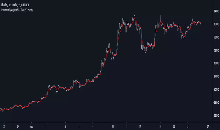
Dynamically Adjustable FilterIntroduction
Inspired from the Kalman filter this indicator aim to provide a good result in term of smoothness and reactivity while letting the user the option to increase/decrease smoothing.
Optimality And Dynamical Adjustment
This indicator is constructed in the same manner as many adaptive moving averages by using exponential averaging with a smoothing variable, this is described by :
x= x_1 + a(y - x_1)
where y is the input price (measurements) and a is the smoothing variable, with Kalman filters a is often replaced by K or Kalman Gain , this Gain is what adjust the estimate to the measurements. In the indicator K is calculated as follow :
K = Absolute Error of the estimate/(Absolute Error of the estimate + Measurements Dispersion * length)
The error of the estimate is just the absolute difference between the measurements and the estimate, the dispersion is the measurements standard deviation and length is a parameter controlling smoothness. K adjust to price volatility and try to provide a good estimate no matter the size of length . In order to increase reactivity the price input (measurements) has been summed with the estimate error.
Now this indicator use a fraction of what a Kalman filter use for its entire calculation, therefore the covariance update has been discarded as well as the extrapolation part.
About parameters length control the filter smoothness, the lag reduction option create more reactive results.
Conclusion
You can create smoothing variables for any adaptive indicator by using the : a/(a+b) form since this operation always return values between 0 and 1 as long as a and b are positive. Hope it help !
Thanks for reading !
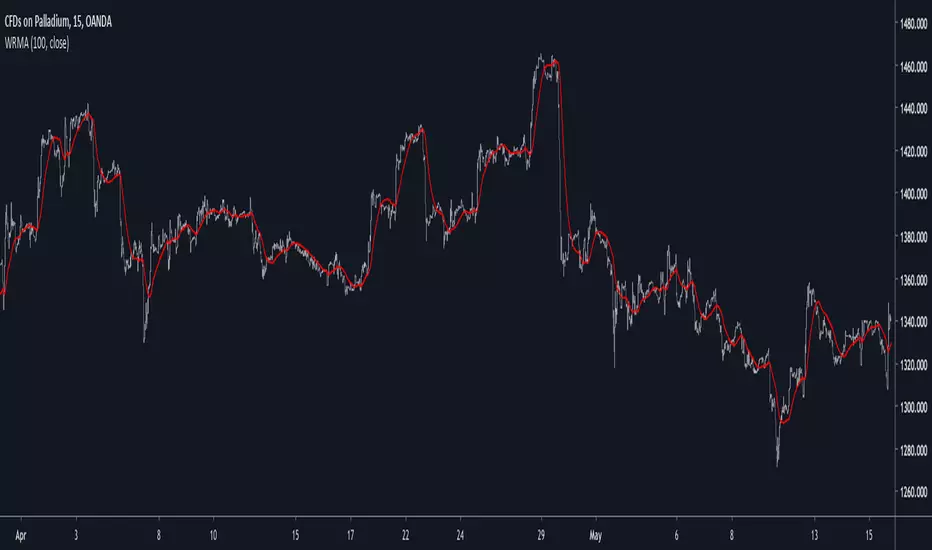
Well Rounded Moving AverageIntroduction
There are tons of filters, way to many, and some of them are redundant in the sense they produce the same results as others. The task to find an optimal filter is still a big challenge among technical analysis and engineering, a good filter is the Kalman filter who is one of the more precise filters out there. The optimal filter theorem state that : The optimal estimator has the form of a linear observer , this in short mean that an optimal filter must use measurements of the inputs and outputs, and this is what does the Kalman filter. I have tried myself to Kalman filters with more or less success as well as understanding optimality by studying Linear–quadratic–Gaussian control, i failed to get a complete understanding of those subjects but today i present a moving average filter (WRMA) constructed with all the knowledge i have in control theory and who aim to provide a very well response to market price, this mean low lag for fast decision timing and low overshoots for better precision.
Construction
An good filter must use information about its output, this is what exponential smoothing is about, simple exponential smoothing (EMA) is close to a simple moving average and can be defined as :
output = output(1) + α(input - output(1))
where α (alpha) is a smoothing constant, typically equal to 2/(Period+1) for the EMA.
This approach can be further developed by introducing more smoothing constants and output control (See double/triple exponential smoothing - alpha-beta filter) .
The moving average i propose will use only one smoothing constant, and is described as follow :
a = nz(a ) + alpha*nz(A )
b = nz(b ) + alpha*nz(B )
y = ema(a + b,p1)
A = src - y
B = src - ema(y,p2)
The filter is divided into two components a and b (more terms can add more control/effects if chosen well) , a adjust itself to the output error and is responsive while b is independent of the output and is mainly smoother, adding those components together create an output y , A is the output error and B is the error of an exponential moving average.
Comparison
There are a lot of low-lag filters out there, but the overshoots they induce in order to reduce lag is not a great effect. The first comparison is with a least square moving average, a moving average who fit a line in a price window of period length .
Lsma in blue and WRMA in red with both length = 100 . The lsma is a bit smoother but induce terrible overshoots
ZLMA in blue and WRMA in red with both length = 100 . The lag difference between each moving average is really low while VWRMA is way more precise.
Hull MA in blue and WRMA in red with both length = 100 . The Hull MA have similar overshoots than the LSMA.
Reduced overshoots moving average (ROMA) in blue and WRMA in red with both length = 100 . ROMA is an indicator i have made to reduce the overshoots of a LSMA, but at the end WRMA still reduce way more the overshoots while being smoother and having similar lag.
I have added a smoother version, just activate the extra smooth option in the indicator settings window. Here the result with length = 200 :
This result is a little bit similar to a 2 order Butterworth filter. Our filter have more overshoots which in this case could be useful to reduce the error with edges since other low pass filters tend to smooth their amplitude thus reducing edge estimation precision.
Conclusions
I have presented a well rounded filter in term of smoothness/stability and reactivity. Try to add more terms to have different results, you could maybe end up with interesting results, if its the case share them with the community :)
As for control theory i have seen neural networks integrated to Kalman flters which leaded to great accuracy, AI is everywhere and promise to be a game a changer in real time data smoothing. So i asked myself if it was possible for a neural networks to develop pinescript indicators, if yes then i could be replaced by AI ? Brrr how frightening.
Thanks for reading :)
Multi Poles Zero-Lag Exponential Moving AverageIntroduction
Based on the exponential averaging method with lag reduction, this filter allow for smoother results thanks to a multi-poles approach. Translated and modified from the Non-Linear Kalman Filter from Mladen Rakic 01/07/19 www.mql5.com
The Indicator
length control the amount of smoothing, the poles can be from 1 to 3, higher values create smoother results.
Difference With Classic Exponential Smoothing
A classic 1 depth recursion (Single smoothing) exponential moving average is defined as y = αx + (1 - α)y which can be derived into y = y + α(x - y )
2 depth recursion (Double smoothing) exponential moving average sum y with b in order to reduce the error with x , this method is calculated as follow :
y = αx + (1 - α)(y + b)
b = β(y - y ) + (1-β)b
The initial value for y is x while its 0 for b with α generally equal to 2/(length + 1)
The filter use a different approach, from the estimation of α/β/γ to the filter construction.The formula is similar to the one used in the double exponential smoothing method with a difference in y and b
y = αx + (1 - α)y
d = x - y
b = (1-β)b + d
output = y + b
instead of updating y with b the two components are directly added in a separated variable. Poles help the transition band of the frequency response to get closer to the cutoff point, the cutoff of an exponential moving average is defined as :
Cf = F/2π acos(1 - α*α/(2(1 - α)))
Also in order to minimize the overshoot of the filter a correction has been added to the output now being output = y + 1/poles * b
While this information is far being helpful to you it simply say that poles help you filter a great amount of noise thus removing irregularities of the filter.
Conclusion
The filter is interesting and while being similar to multi-depth recursion smoothing allow for more varied results thanks to its 3 poles.
Feel free to send suggestions :)
Thanks for reading
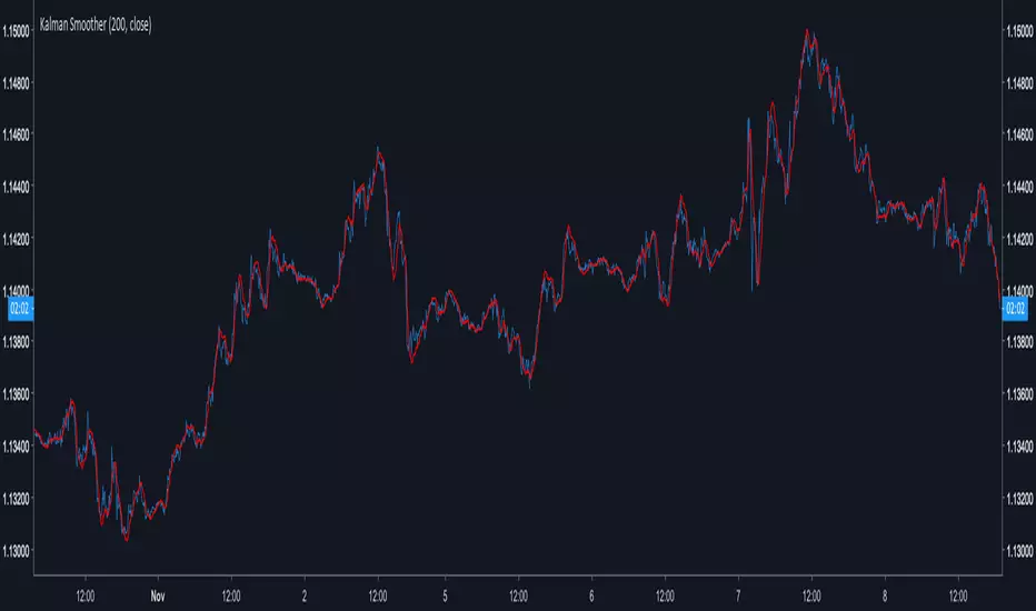
Kalman SmootherA derivation of the Kalman Filter.
Lower Gain values create smoother results.The ratio Smoothing/Lag is similar to any Low Lagging Filters.
The Gain parameter can be decimal numbers.
Kalman Smoothing With Gain = 20
For any questions/suggestions feel free to contact me
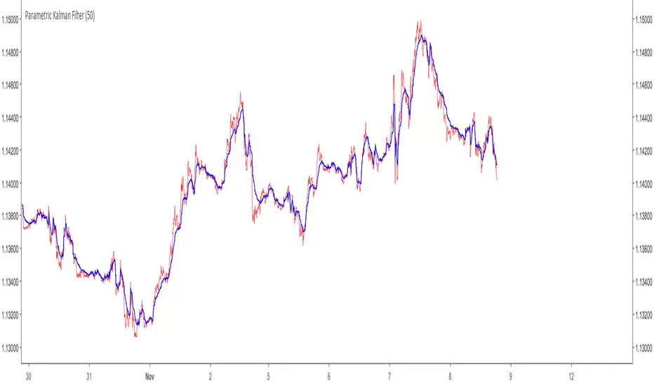
One Dimensional Parametric Kalman FilterA One Dimensional Kalman Filter, the particularity of Kalman Filtering is the constant recalculation of the Error between the measurements and the estimate.This version is modified to allow more/less filtering using an alternative calculation of the error measurement.
Camparison of the Kalman filter Red with a moving average Black of both period 50
Can be used as source for others indicators such as stochastic/rsi/moving averages...etc
For any questions/suggestions feel free to contact me