Ripster Labels + Air Gaps (v6)What it shows (on one chart)
EMA Clouds (current timeframe)
Plots EMA 8/12/21/34/50/200 with three cloud fills:
12–21 = “fast” cloud
34–50 = “mid” cloud
50–200 = “base” cloud
Cloud color: green when the faster EMA is above the slower (bullish), red/maroon/orange when below (bearish).
Toggle lines vs. clouds via A) EMA Clouds settings.
MTF Rails (higher-TF EMAs)
For three higher timeframes (defaults 30m / 60m / 240m), draws two EMAs each (defaults 34 & 50).
These are stepline-like rails you can visually use as higher-TF supports/resistances.
Configure in B) MTF Rails (turn on/off, change TFs/lengths/colors).
Relative Volume Box (RVol)
Small table (top-center) showing:
Candle Vol (formatted K/M/B if enabled)
RVol = current bar volume / SMA 20 of volume (as a %)
Color scale: blue (<100%), yellow (100–150%), red (>150%).
Settings in C) RVol Box.
DTR vs ATR Box
Daily True Range (DTR = day high − day low) vs ATR(14) on the daily timeframe, with DTR as % of ATR.
Placed at top-right; toggle in D) DTR/ATR Box.
Ripster Trend Label (10m 12/50)
Looks at a separate timeframe (default 10m): EMA 12 vs EMA 50.
Bottom-right table cell shows “10m Trend ↑/↓/Sideways” (green/red/gray).
Configure in E) Ripster Trend Labels (TF and lengths).
Air Gaps (single EMA per TF)
Three horizontal, auto-extending lines showing an EMA from 30m / 60m / 240m (default length 12).
“Air gaps” are the price spaces between these lines—often lighter-resistance zones for price.
Start point logic:
All Bars = draw from the chart’s left
Start of Day = draw from today’s first bar
Bars Offset = draw from N bars back (default 100)
Settings in F) Air Gaps (TFs, length, draw-from, bars-back).
Inputs & where to tweak
A) EMA Clouds
Show EMA Clouds: master toggle
Source: close (default)
Lengths: 8/12/21/34/50/200
Show EMA lines: toggle plotted lines (clouds remain)
B) MTF Rails
Show MTF Rails
TF1/TF2/TF3 (defaults 30/60/240)
EMA A/B (defaults 34/50)
C) RVol Box
Show box
Format as K/M/B: K=1e3, M=1e6, B=1e9
D) DTR/ATR Box
Show DTR/ATR
ATR len: default 14 (daily)
E) Ripster Trend Labels
Show labels
Trend TF: default 10 (10-minute)
Trend EMA Fast/Slow: default 12/50
F) Air Gaps
Show Air Gap lines
TF1/TF2/TF3 (30/60/240)
EMA length: default 12
Draw from: All Bars | Start of Day | Bars Offset
Bars back: used if Draw from = Bars Offset
How it makes decisions
Cloud bias = sign of (faster EMA − slower EMA) for each cloud pair.
Example: 12>21 → fast cloud is bullish (green); 34>50 → mid cloud bullish (teal).
10m trend label = sign of (EMA12−EMA50) on the Trend TF (default 10m).
RVol = volume / sma(volume, 20); formatted as a percent and color-coded.
Practical read of the screen
Fast cloud flips (12/21) often mark short-term momentum changes; mid cloud flips (34/50) reflect swing bias.
Air Gap lines from higher TFs frequently act as support/resistance. Larger spaces between lines = “air gaps” where price can move with less friction.
RVol color tells you how “real” a move is: red/yellow often confirms momentum; blue warns of thin/liquidy bars.
DTR vs ATR shows if today’s range is stretched vs recent norm.
Design choices (why your prior errors are gone)
Removed multiline ?: chains → replaced by if/else (Pine v6 is picky about line continuations).
Moved fill() calls outside of local if blocks (Pine limitation).
ta.change(time("D")) != 0 makes the if condition boolean.
Declared G_drawFrom / G_barsBack before startX() so identifiers exist.
Cerca negli script per "12月4号是什么星座"

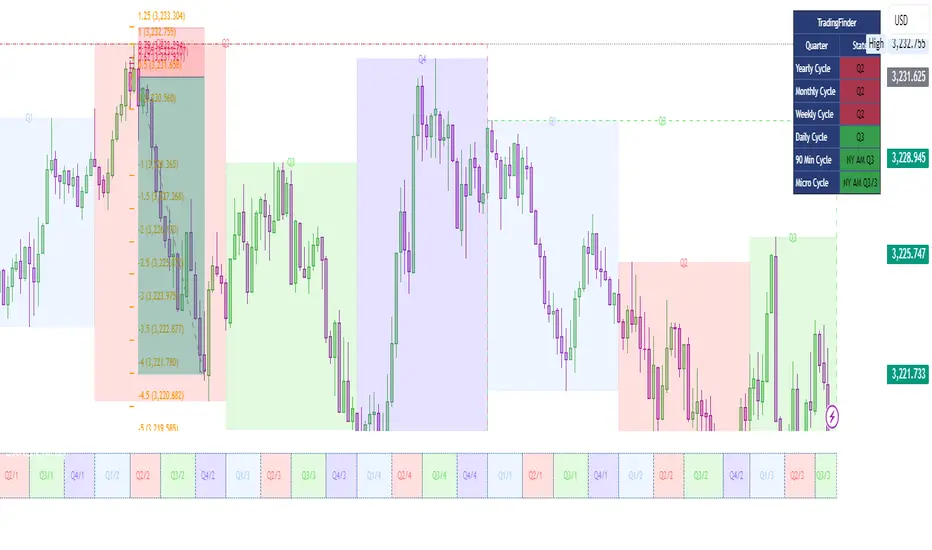
Quarterly Cycle Theory with DST time AdjustedThe Quarterly Theory removes ambiguity, as it gives specific time-based reference points to look for when entering trades. Before being able to apply this theory to trading, one must first understand that time is fractal:
Yearly Quarters = 4 quarters of three months each.
Monthly Quarters = 4 quarters of one week each.
Weekly Quarters = 4 quarters of one day each (Monday - Thursday). Friday has its own specific function.
Daily Quarters = 4 quarters of 6 hours each = 4 trading sessions of a trading day.
Sessions Quarters = 4 quarters of 90 minutes each.
90 Minute Quarters = 4 quarters of 22.5 minutes each.
Yearly Cycle: Analogously to financial quarters, the year is divided in four sections of three months each:
Q1 - January, February, March.
Q2 - April, May, June (True Open, April Open).
Q3 - July, August, September.
Q4 - October, November, December.
S&P 500 E-mini Futures (daily candles) — Monthly Cycle.
Monthly Cycle: Considering that we have four weeks in a month, we start the cycle on the first month’s Monday (regardless of the calendar Day):
Q1 - Week 1: first Monday of the month.
Q2 - Week 2: second Monday of the month (True Open, Daily Candle Open Price).
Q3 - Week 3: third Monday of the month.
Q4 - Week 4: fourth Monday of the month.
S&P 500 E-mini Futures (4 hour candles) — Weekly Cycle.
Weekly Cycle: Daye determined that although the trading week is composed by 5 trading days, we should ignore Friday, and the small portion of Sunday’s price action:
Q1 - Monday.
Q2 - Tuesday (True Open, Daily Candle Open Price).
Q3 - Wednesday.
Q4 - Thursday.
S&P 500 E-mini Futures (1 hour candles) — Daily Cycle.
Daily Cycle: The Day can be broken down into 6 hour quarters. These times roughly define the sessions of the trading day, reinforcing the theory’s validity:
Q1 - 18:00 - 00:00 Asia.
Q2 - 00:00 - 06:00 London (True Open).
Q3 - 06:00 - 12:00 NY AM.
Q4 - 12:00 - 18:00 NY PM.
S&P 500 E-mini Futures (15 minute candles) — 6 Hour Cycle.
6 Hour Quarters or 90 Minute Cycle / Sessions divided into four sections of 90 minutes each (EST/EDT):
Asian Session
Q1 - 18:00 - 19:30
Q2 - 19:30 - 21:00 (True Open)
Q3 - 21:00 - 22:30
Q4 - 22:30 - 00:00
London Session
Q1 - 00:00 - 01:30
Q2 - 01:30 - 03:00 (True Open)
Q3 - 03:00 - 04:30
Q4 - 04:30 - 06:00
NY AM Session
Q1 - 06:00 - 07:30
Q2 - 07:30 - 09:00 (True Open)
Q3 - 09:00 - 10:30
Q4 - 10:30 - 12:00
NY PM Session
Q1 - 12:00 - 13:30
Q2 - 13:30 - 15:00 (True Open)
Q3 - 15:00 - 16:30
Q4 - 16:30 - 18:00
S&P 500 E-mini Futures (5 minute candles) — 90 Minute Cycle.
Micro Cycles: Dividing the 90 Minute Cycle yields 22.5 Minute Quarters, also known as Micro Sessions or Micro Quarters:
Asian Session
Q1/1 18:00:00 - 18:22:30
Q2 18:22:30 - 18:45:00
Q3 18:45:00 - 19:07:30
Q4 19:07:30 - 19:30:00
Q2/1 19:30:00 - 19:52:30 (True Session Open)
Q2/2 19:52:30 - 20:15:00
Q2/3 20:15:00 - 20:37:30
Q2/4 20:37:30 - 21:00:00
Q3/1 21:00:00 - 21:23:30
etc. 21:23:30 - 21:45:00
London Session
00:00:00 - 00:22:30 (True Daily Open)
00:22:30 - 00:45:00
00:45:00 - 01:07:30
01:07:30 - 01:30:00
01:30:00 - 01:52:30 (True Session Open)
01:52:30 - 02:15:00
02:15:00 - 02:37:30
02:37:30 - 03:00:00
03:00:00 - 03:22:30
03:22:30 - 03:45:00
03:45:00 - 04:07:30
04:07:30 - 04:30:00
04:30:00 - 04:52:30
04:52:30 - 05:15:00
05:15:00 - 05:37:30
05:37:30 - 06:00:00
New York AM Session
06:00:00 - 06:22:30
06:22:30 - 06:45:00
06:45:00 - 07:07:30
07:07:30 - 07:30:00
07:30:00 - 07:52:30 (True Session Open)
07:52:30 - 08:15:00
08:15:00 - 08:37:30
08:37:30 - 09:00:00
09:00:00 - 09:22:30
09:22:30 - 09:45:00
09:45:00 - 10:07:30
10:07:30 - 10:30:00
10:30:00 - 10:52:30
10:52:30 - 11:15:00
11:15:00 - 11:37:30
11:37:30 - 12:00:00
New York PM Session
12:00:00 - 12:22:30
12:22:30 - 12:45:00
12:45:00 - 13:07:30
13:07:30 - 13:30:00
13:30:00 - 13:52:30 (True Session Open)
13:52:30 - 14:15:00
14:15:00 - 14:37:30
14:37:30 - 15:00:00
15:00:00 - 15:22:30
15:22:30 - 15:45:00
15:45:00 - 15:37:30
15:37:30 - 16:00:00
16:00:00 - 16:22:30
16:22:30 - 16:45:00
16:45:00 - 17:07:30
17:07:30 - 18:00:00
S&P 500 E-mini Futures (30 second candles) — 22.5 Minute Cycle.
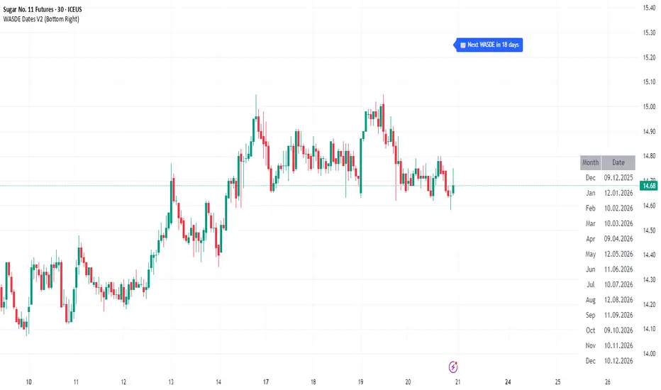
WASDE Dates V2WASDE Dates V2 – USDA Release Calendar with Alerts, Countdown & Event Markers
By cot-trader.com
WASDE Dates V2 is a complete and reliable visualization tool for all scheduled WASDE (World Agricultural Supply and Demand Estimates) releases for 2025 and 2026.
The USDA’s WASDE report is one of the most market-moving fundamental catalysts in agricultural futures—affecting Corn (ZC), Wheat (ZW), Soybeans (ZS), Soymeal (ZM), Soybean Oil (ZL), and many related CFD products.
This script gives traders a precise timing layer directly inside their TradingView charts.
🔍 What this script does
WASDE Dates V2 automatically:
Marks each WASDE release day with a vertical line and label.
Shows an automated countdown to the next WASDE release:
In days (>24h)
In hours & minutes (<24h)
Displays an optional table of upcoming WASDE dates for quick reference.
Provides two alert conditions:
WASDE Day Alert – triggers exactly on the event
WASDE 24h Reminder – pre-alert when less than 24 hours remain
Handles both 2025 and 2026 confirmed dates.
Works on any symbol and timeframe.
📌 Why WASDE matters
The WASDE report updates global supply and demand estimates for:
Corn
Soybeans
Wheat
Other major agricultural commodities
Changes in yield, acres, production, imports/exports, and ending stocks can cause immediate and significant volatility.
Many traders combine WASDE awareness with seasonality, COT positioning, volatility filters, or fundamental models.
This script ensures you never miss the timing of these key releases.
⚙️ How the script works
The script stores official USDA WASDE release dates for 2025 and 2026 in two dedicated arrays.
On every bar, it compares the bar’s timestamp with known WASDE timestamps to detect an event day.
When an event occurs:
A red “WASDE” label is plotted above the candle
A dotted vertical line is drawn through the bar
It finds the next upcoming WASDE by scanning forward through both arrays.
A live-updating countdown label is displayed, showing days or hours/minutes until release.
If the event is less than 24 hours away:
A yellow “WASDE soon” warning appears near price
The 24h alert condition becomes active
An optional table lists upcoming events for 2025 & 2026.
This script does not generate trading signals.
It provides a time-based event layer designed to complement any discretionary or algorithmic trading approach.
🧭 How to use
Add the script to your chart.
Enable alerts for:
“WASDE Day Alert”
“WASDE 24h Reminder”
Follow the countdown to prepare for upcoming volatility.
Use together with other agricultural tools such as:
Seasonality indicators
COT (Commitment of Traders) analysis
Trend / VWAP / Volume signals
Pre- and post-WASDE trading strategies
Works on all chart types, all symbols, and all timeframes.
📅 Included WASDE Dates (Confirmed)
2025:
Jan 12, Feb 11, Mar 11, Apr 10, May 12, Jun 12, Jul 11, Aug 12, Sep 12, Oct 9, Nov 10, Dec 9
2026:
Jan 12, Feb 10, Mar 10, Apr 9, May 12, Jun 11, Jul 10, Aug 12, Sep 11, Oct 9, Nov 10, Dec 10
(All dates based on USDA’s official 12:00pm ET schedule.)
💡 What makes this script original
Fully updated 2025 + 2026 calendar
Uses a robust time-comparison method for accurate marking
Unique dual alert system (event + 24h pre-alert)
Clean, readable layout with countdown + upcoming dates table
Tailored specifically for grain & agricultural traders
Built entirely in Pine Script v6 with careful attention to performance
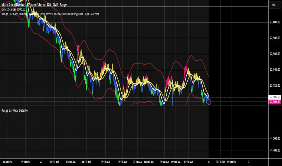
Range Bar Gaps DetectorRange Bar Gaps Detector
Overview
The Range Bar Gaps Detector identifies price gaps across multiple range bar sizes (12, 24, 60, and 120) on any trading instrument, helping traders spot potential support/resistance zones or breakout opportunities. Designed for Pine Script v6, this indicator detects gaps on range bars and exports data for use in companion scripts like Range Bar Gaps Overlap, making it ideal for multi-timeframe gap analysis.
Key Features
Multi-Range Gap Detection: Identifies gaps on 12, 24, 60, and 120-range bars, capturing both bullish (gap up) and bearish (gap down) price movements.
Customizable Sensitivity: Includes a user-defined minimum deviation (default: 10% of 14-period SMA) for 12-range gaps to filter out noise.
7-Day Lookback: Automatically prunes gaps older than 7 days to focus on recent, relevant price levels.
Data Export: Serializes up to 10 gaps per range (tops, bottoms, start bars, highest/lowest prices, and age) for seamless integration with overlap analysis scripts.
Debugging Support: Plots gap counts and aggregation data in the Data Window for easy verification of detected gaps.
How It Works
The indicator aggregates price movements to simulate higher range bars (24, 60, 120) from a base range bar chart. It detects gaps when the price jumps significantly between bars, ensuring gaps meet the minimum deviation threshold for 12-range bars. Gaps are stored in arrays, serialized for external use, and pruned after 7 days to maintain efficiency.
Usage
Add to your range bar chart (e.g., 12-range) to detect gaps across multiple ranges.
Use alongside the Range Bar Gaps Overlap indicator to visualize gaps and their overlaps as boxes on the chart.
Check the Data Window to confirm gap counts and sizes for each range (12, 24, 60, 120).
Adjust the "Minimal Deviation (%) for 12-Range" input to control gap detection sensitivity.
Settings
Minimal Deviation (%) for 12-Range: Set the minimum gap size for 12-range bars (default: 10% of 14-period SMA).
Range Sizes: Fixed at 24, 60, and 120 for higher range bar aggregation.
Notes
Ensure the script is published under your TradingView username (e.g., GreenArrow2005) for use with companion scripts.
Best used on range bar charts to maintain consistent gap detection.
For advanced overlap analysis, pair with the Range Bar Gaps Overlap indicator to highlight zones where gaps from different ranges align.
Ideal For
Traders seeking to identify key price levels for support/resistance or breakout strategies.
Multi-timeframe analysts combining gap data across various range bar sizes.
Developers building custom indicators that leverage gap data for advanced charting.
2:30 [LuciTech]this is a technical analysis tool designed to highlight key price levels and patterns during a specific trading window, based on UK time (Europe/London). It overlays visual elements on the chart, including a 12 PM reference line, Buy Side Liquidity (BSL) and Sell Side Liquidity (SSL) levels, a highlighted 2:30 PM candle, and Engulfing Fair Value Gaps (FVGs). This indicator is intended for traders who focus on intraday price action and liquidity zones.
Features
The 12 PM Line displays a vertical line at 12:00 PM (UK time) to mark the start of the session. It’s customizable, allowing you to enable or disable it and adjust its color.
BSL/SSL Lines track the highest high (BSL) and lowest low (SSL) from 12:00 PM to 2:00 PM (UK time). These lines extend horizontally until 3:30 PM, after which they remain static at their last recorded levels. You can customize them by enabling or disabling visibility, adjusting colors, choosing a line style (solid, dashed, or dotted), and setting the width.
The 2:30 PM Candle highlights the candle at 2:30 PM (UK time) with a distinct color. It’s customizable, with options to enable or disable it and change its color.
Engulfing FVG (Fair Value Gap) identifies bullish and bearish engulfing patterns with a gap from the prior candle’s range. It draws a shaded box over the FVG area, and you can customize it by enabling or disabling it and adjusting the box color.
How It Works
The indicator operates within a session starting at 12:00 PM (UK time). BSL/SSL levels update between 12:00 PM and 2:00 PM, with lines extending until 3:30 PM. After 3:30 PM, these lines freeze.
BSL/SSL lines show the highest price (BSL) and lowest price (SSL) reached during the 12:00 PM to 2:00 PM window. After 3:30 PM, they remain static, marking the final range boundaries.
The 2:30 PM candle emphasizes a key timestamp, often of interest to intraday traders.
Engulfing FVGs detect significant price gaps created by engulfing candles, which may indicate potential reversal or continuation zones.
Settings
12 PM Line Settings let you toggle visibility and set the line color.
BSL/SSL Line Settings allow you to toggle visibility, set BSL and SSL colors, choose a line style (Solid, Dashed, Dotted), and adjust width (1-4).
2:30 Candle Settings let you toggle visibility and set the candle color.
Engulfing FVG Settings allow you to toggle visibility and set the box color.
Interpretation
The 12 PM Line serves as a reference for the session start.
BSL/SSL Lines may act as potential support or resistance zones or highlight liquidity areas. After 3:30 PM, they remain static, showing the session’s final range.
The 2:30 PM Candle can be monitored for price action signals, such as reversals or breakouts.
Engulfing FVGs shaded areas may indicate imbalances in supply and demand, useful for identifying trade opportunities or stop-loss placement.
Notes
The timezone is set to Europe/London (UK time). Ensure your chart’s timezone aligns for accurate results.
This indicator is best used on intraday timeframes, such as 1-minute or 5-minute charts.
It provides visual aids for analysis and does not generate buy or sell signals on its own.

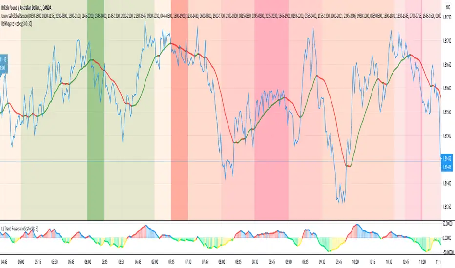
Universal Global SessionUniversal Global Session
This Script combines the world sessions of: Stocks, Forex, Bitcoin Kill Zones, strategic points, all configurable, in a single Script, to capitalize the opening and closing times of global exchanges as investment assets, becoming an Universal Global Session .
It is based on the great work of @oscarvs ( BITCOIN KILL ZONES v2 ) and the scripts of @ChrisMoody. Thank you Oscar and Chris for your excellent judgment and great work.
At the end of this writing you can find all the internet references of the extensive documentation that I present here. To maximize your benefits in the use of this Script, I recommend that you read the entire document to create an objective and practical criterion.
All the hours of the different exchanges are presented at GMT -6. In Market24hClock you can adjust it to your preferences.
After a deep investigation I have been able to show that the different world sessions reveal underlying investment cycles, where it is possible to find sustained changes in the nominal behavior of the trend before the passage from one session to another and in the natural overlaps between the sessions. These underlying movements generally occur 15 minutes before the start, close or overlap of the session, when the session properly starts and also 15 minutes after respectively. Therefore, this script is designed to highlight these particular trending behaviors. Try it, discover your own conclusions and let me know in the notes, thank you.
Foreign Exchange Market Hours
It is the schedule by which currency market participants can buy, sell, trade and speculate on currencies all over the world. It is open 24 hours a day during working days and closes on weekends, thanks to the fact that operations are carried out through a network of information systems, instead of physical exchanges that close at a certain time. It opens Monday morning at 8 am local time in Sydney —Australia— (which is equivalent to Sunday night at 7 pm, in New York City —United States—, according to Eastern Standard Time), and It closes at 5pm local time in New York City (which is equivalent to 6am Saturday morning in Sydney).
The Forex market is decentralized and driven by local sessions, where the hours of Forex trading are based on the opening range of each active country, becoming an efficient transfer mechanism for all participants. Four territories in particular stand out: Sydney, Tokyo, London and New York, where the highest volume of operations occurs when the sessions in London and New York overlap. Furthermore, Europe is complemented by major financial centers such as Paris, Frankfurt and Zurich. Each day of forex trading begins with the opening of Australia, then Asia, followed by Europe, and finally North America. As markets in one region close, another opens - or has already opened - and continues to trade in the currency market. The seven most traded currencies in the world are: the US dollar, the euro, the Japanese yen, the British pound, the Australian dollar, the Canadian dollar, and the New Zealand dollar.
Currencies are needed around the world for international trade, this means that operations are not dominated by a single exchange market, but rather involve a global network of brokers from around the world, such as banks, commercial companies, central banks, companies investment management, hedge funds, as well as retail forex brokers and global investors. Because this market operates in multiple time zones, it can be accessed at any time except during the weekend, therefore, there is continuously at least one open market and there are some hours of overlap between the closing of the market of one region and the opening of another. The international scope of currency trading means that there are always traders around the world making and satisfying demands for a particular currency.
The market involves a global network of exchanges and brokers from around the world, although time zones overlap, the generally accepted time zone for each region is as follows:
Sydney 5pm to 2am EST (10pm to 7am UTC)
London 3am to 12 noon EST (8pm to 5pm UTC)
New York 8am to 5pm EST (1pm to 10pm UTC)
Tokyo 7pm to 4am EST (12am to 9am UTC)
Trading Session
A financial asset trading session refers to a period of time that coincides with the daytime trading hours for a given location, it is a business day in the local financial market. This may vary according to the asset class and the country, therefore operators must know the hours of trading sessions for the securities and derivatives in which they are interested in trading. If investors can understand market hours and set proper targets, they will have a much greater chance of making a profit within a workable schedule.
Kill Zones
Kill zones are highly liquid events. Many different market participants often come together and perform around these events. The activity itself can be event-driven (margin calls or option exercise-related activity), portfolio management-driven (asset allocation rebalancing orders and closing buy-in), or institutionally driven (larger players needing liquidity to complete the size) or a combination of any of the three. This intense cross-current of activity at a very specific point in time often occurs near significant technical levels and the established trends emerging from these events often persist until the next Death Zone approaches or enters.
Kill Zones are evolving with time and the course of world history. Since the end of World War II, New York has slowly invaded London's place as the world center for commercial banking. So much so that during the latter part of the 20th century, New York was considered the new center of the financial universe. With the end of the cold war, that leadership appears to have shifted towards Europe and away from the United States. Furthermore, Japan has slowly lost its former dominance in the global economic landscape, while Beijing's has increased dramatically. Only time will tell how these death zones will evolve given the ever-changing political, economic, and socioeconomic influences of each region.
Financial Markets
New York
New York (NYSE Chicago, NASDAQ)
7:30 am - 2:00 pm
It is the second largest currency platform in the world, followed largely by foreign investors as it participates in 90% of all operations, where movements on the New York Stock Exchange (NYSE) can have an immediate effect (powerful) on the dollar, for example, when companies merge and acquisitions are finalized, the dollar can instantly gain or lose value.
A. Complementary Stock Exchanges
Brazil (BOVESPA - Brazilian Stock Exchange)
07:00 am - 02:55 pm
Canada (TSX - Toronto Stock Exchange)
07:30 am - 02:00 pm
New York (NYSE - New York Stock Exchange)
08:30 am - 03:00 pm
B. North American Trading Session
07:00 am - 03:00 pm
(from the beginning of the business day on NYSE and NASDAQ, until the end of the New York session)
New York, Chicago and Toronto (Canada) open the North American session. Characterized by the most aggressive trading within the markets, currency pairs show high volatility. As the US markets open, trading is still active in Europe, however trading volume generally decreases with the end of the European session and the overlap between the US and Europe.
C. Strategic Points
US main session starts in 1 hour
07:30 am
The euro tends to drop before the US session. The NYSE, CHX and TSX (Canada) trading sessions begin 1 hour after this strategic point. The North American session begins trading Forex at 07:00 am.
This constitutes the beginning of the overlap of the United States and the European market that spans from 07:00 am to 10:35 am, often called the best time to trade EUR / USD, it is the period of greatest liquidity for the main European currencies since it is where they have their widest daily ranges.
When New York opens at 07:00 am the most intense trading begins in both the US and European markets. The overlap of European and American trading sessions has 80% of the total average trading range for all currency pairs during US business hours and 70% of the total average trading range for all currency pairs during European business hours. The intersection of the US and European sessions are the most volatile overlapping hours of all.
Influential news and data for the USD are released between 07:30 am and 09:00 am and play the biggest role in the North American Session. These are the strategically most important moments of this activity period: 07:00 am, 08:00 am and 08:30 am.
The main session of operations in the United States and Canada begins
08:30 am
Start of main trading sessions in New York, Chicago and Toronto. The European session still overlaps the North American session and this is the time for large-scale unpredictable trading. The United States leads the market. It is difficult to interpret the news due to speculation. Trends develop very quickly and it is difficult to identify them, however trends (especially for the euro), which have developed during the overlap, often turn the other way when Europe exits the market.
Second hour of the US session and last hour of the European session
09:30 am
End of the European session
10:35 am
The trend of the euro will change rapidly after the end of the European session.
Last hour of the United States session
02:00 pm
Institutional clients and very large funds are very active during the first and last working hours of almost all stock exchanges, knowing this allows to better predict price movements in the opening and closing of large markets. Within the last trading hours of the secondary market session, a pullback can often be seen in the EUR / USD that continues until the opening of the Tokyo session. Generally it happens if there was an upward price movement before 04:00 pm - 05:00 pm.
End of the trade session in the United States
03:00 pm
D. Kill Zones
11:30 am - 1:30 pm
New York Kill Zone. The United States is still the world's largest economy, so by default, the New York opening carries a lot of weight and often comes with a huge injection of liquidity. In fact, most of the world's marketable assets are priced in US dollars, making political and economic activity within this region even more important. Because it is relatively late in the world's trading day, this Death Zone often sees violent price swings within its first hour, leading to the proven adage "never trust the first hour of trading in America. North.
---------------
London
London (LSE - London Stock Exchange)
02:00 am - 10:35 am
Britain dominates the currency markets around the world, and London is its main component. London, a central trading capital of the world, accounts for about 43% of world trade, many Forex trends often originate from London.
A. Complementary Stock Exchange
Dubai (DFM - Dubai Financial Market)
12:00 am - 03:50 am
Moscow (MOEX - Moscow Exchange)
12:30 am - 10:00 am
Germany (FWB - Frankfurt Stock Exchange)
01:00 am - 10:30 am
Afríca (JSE - Johannesburg Stock Exchange)
01:00 am - 09:00 am
Saudi Arabia (TADAWUL - Saudi Stock Exchange)
01:00 am - 06:00 am
Switzerland (SIX - Swiss Stock Exchange)
02:00 am - 10:30 am
B. European Trading Session
02:00 am - 11:00 am
(from the opening of the Frankfurt session to the close of the Order Book on the London Stock Exchange / Euronext)
It is a very liquid trading session, where trends are set that start during the first trading hours in Europe and generally continue until the beginning of the US session.
C. Middle East Trading Session
12:00 am - 06:00 am
(from the opening of the Dubai session to the end of the Riyadh session)
D. Strategic Points
European session begins
02:00 am
London, Frankfurt and Zurich Stock Exchange enter the market, overlap between Europe and Asia begins.
End of the Singapore and Asia sessions
03:00 am
The euro rises almost immediately or an hour after Singapore exits the market.
Middle East Oil Markets Completion Process
05:00 am
Operations are ending in the European-Asian market, at which time Dubai, Qatar and in another hour in Riyadh, which constitute the Middle East oil markets, are closing. Because oil trading is done in US dollars, and the region with the trading day coming to an end no longer needs the dollar, consequently, the euro tends to grow more frequently.
End of the Middle East trading session
06:00 am
E. Kill Zones
5:00 am - 7:00 am
London Kill Zone. Considered the center of the financial universe for more than 500 years, Europe still has a lot of influence in the banking world. Many older players use the European session to establish their positions. As such, the London Open often sees the most significant trend-setting activity on any trading day. In fact, it has been suggested that 80% of all weekly trends are set through the London Kill Zone on Tuesday.
F. Kill Zones (close)
2:00 pm - 4:00 pm
London Kill Zone (close).
---------------
Tokyo
Tokyo (JPX - Tokyo Stock Exchange)
06:00 pm - 12:00 am
It is the first Asian market to open, receiving most of the Asian trade, just ahead of Hong Kong and Singapore.
A. Complementary Stock Exchange
Singapore (SGX - Singapore Exchange)
07:00 pm - 03:00 am
Hong Kong (HKEx - Hong Kong Stock Exchange)
07:30 pm - 02:00 am
Shanghai (SSE - Shanghai Stock Exchange)
07:30 pm - 01:00 am
India (NSE - India National Stock Exchange)
09:45 pm - 04:00 am
B. Asian Trading Session
06:00 pm - 03:00 am
From the opening of the Tokyo session to the end of the Singapore session
The first major Asian market to open is Tokyo which has the largest market share and is the third largest Forex trading center in the world. Singapore opens in an hour, and then the Chinese markets: Shanghai and Hong Kong open 30 minutes later. With them, the trading volume increases and begins a large-scale operation in the Asia-Pacific region, offering more liquidity for the Asian-Pacific currencies and their crosses. When European countries open their doors, more liquidity will be offered to Asian and European crossings.
C. Strategic Points
Second hour of the Tokyo session
07:00 pm
This session also opens the Singapore market. The commercial dynamics grows in anticipation of the opening of the two largest Chinese markets in 30 minutes: Shanghai and Hong Kong, within these 30 minutes or just before the China session begins, the euro usually falls until the same moment of the opening of Shanghai and Hong Kong.
Second hour of the China session
08:30 pm
Hong Kong and Shanghai start trading and the euro usually grows for more than an hour. The EUR / USD pair mixes up as Asian exporters convert part of their earnings into both US dollars and euros.
Last hour of the Tokyo session
11:00 pm
End of the Tokyo session
12:00 am
If the euro has been actively declining up to this time, China will raise the euro after the Tokyo shutdown. Hong Kong, Shanghai and Singapore remain open and take matters into their own hands causing the growth of the euro. Asia is a huge commercial and industrial region with a large number of high-quality economic products and gigantic financial turnover, making the number of transactions on the stock exchanges huge during the Asian session. That is why traders, who entered the trade at the opening of the London session, should pay attention to their terminals when Asia exits the market.
End of the Shanghai session
01:00 am
The trade ends in Shanghai. This is the last trading hour of the Hong Kong session, during which market activity peaks.
D. Kill Zones
10:00 pm - 2:00 am
Asian Kill Zone. Considered the "Institutional" Zone, this zone represents both the launch pad for new trends as well as a recharge area for the post-American session. It is the beginning of a new day (or week) for the world and as such it makes sense that this zone often sets the tone for the remainder of the global business day. It is ideal to pay attention to the opening of Tokyo, Beijing and Sydney.
--------------
Sidney
Sydney (ASX - Australia Stock Exchange)
06:00 pm - 12:00 am
A. Complementary Stock Exchange
New Zealand (NZX - New Zealand Stock Exchange)
04:00 pm - 10:45 pm
It's where the global trading day officially begins. While it is the smallest of the megamarkets, it sees a lot of initial action when markets reopen Sunday afternoon as individual traders and financial institutions are trying to regroup after the long hiatus since Friday afternoon. On weekdays it constitutes the end of the current trading day where the change in the settlement date occurs.
B. Pacific Trading Session
04:00 pm - 12:00 am
(from the opening of the Wellington session to the end of the Sydney session)
Forex begins its business hours when Wellington (New Zealand Exchange) opens local time on Monday. Sydney (Australian Stock Exchange) opens in 2 hours. It is a session with a fairly low volatility, configuring itself as the calmest session of all. Strong movements appear when influential news is published and when the Pacific session overlaps the Asian Session.
C. Strategic Points
End of the Sydney session
12:00 am
---------------
Conclusions
The best time to trade is during overlaps in trading times between open markets. Overlaps equate to higher price ranges, creating greater opportunities.
Regarding press releases (news), it should be noted that these in the currency markets have the power to improve a normally slow trading period. When a major announcement is made regarding economic data, especially when it goes against the predicted forecast, the coin can lose or gain value in a matter of seconds. In general, the more economic growth a country produces, the more positive the economy is for international investors. Investment capital tends to flow to countries that are believed to have good growth prospects and subsequently good investment opportunities, leading to the strengthening of the country's exchange rate. Also, a country that has higher interest rates through its government bonds tends to attract investment capital as foreign investors seek high-yield opportunities. However, stable economic growth and attractive yields or interest rates are inextricably intertwined. It's important to take advantage of market overlaps and keep an eye out for press releases when setting up a trading schedule.
References:
www.investopedia.com
www.investopedia.com
www.investopedia.com
www.investopedia.com
market24hclock.com
market24hclock.com
ORB Fusion🎯 CORE INNOVATION: INSTITUTIONAL ORB FRAMEWORK WITH FAILED BREAKOUT INTELLIGENCE
ORB Fusion represents a complete institutional-grade Opening Range Breakout system combining classic Market Profile concepts (Initial Balance, day type classification) with modern algorithmic breakout detection, failed breakout reversal logic, and comprehensive statistical tracking. Rather than simply drawing lines at opening range extremes, this system implements the full trading methodology used by professional floor traders and market makers—including the critical concept that failed breakouts are often higher-probability setups than successful breakouts .
The Opening Range Hypothesis:
The first 30-60 minutes of trading establishes the day's value area —the price range where the majority of participants agree on fair value. This range is formed during peak information flow (overnight news digestion, gap reactions, early institutional positioning). Breakouts from this range signal directional conviction; failures to hold breakouts signal trapped participants and create exploitable reversals.
Why Opening Range Matters:
1. Information Aggregation : Opening range reflects overnight news, pre-market sentiment, and early institutional orders. It's the market's initial "consensus" on value.
2. Liquidity Concentration : Stop losses cluster just outside opening range. Breakouts trigger these stops, creating momentum. Failed breakouts trap traders, forcing reversals.
3. Statistical Persistence : Markets exhibit range expansion tendency —when price accepts above/below opening range with volume, it often extends 1.0-2.0x the opening range size before mean reversion.
4. Institutional Behavior : Large players (market makers, institutions) use opening range as reference for the day's trading plan. They fade extremes in rotation days and follow breakouts in trend days.
Historical Context:
Opening Range Breakout methodology originated in commodity futures pits (1970s-80s) where floor traders noticed consistent patterns: the first 30-60 minutes established a "fair value zone," and directional moves occurred when this zone was violated with conviction. J. Peter Steidlmayer formalized this observation in Market Profile theory, introducing the "Initial Balance" concept—the first hour (two 30-minute periods) defining market structure.
📊 OPENING RANGE CONSTRUCTION
Four ORB Timeframe Options:
1. 5-Minute ORB (0930-0935 ET):
Captures immediate market direction during "opening drive"—the explosive first few minutes when overnight orders hit the tape.
Use Case:
• Scalping strategies
• High-frequency breakout trading
• Extremely liquid instruments (ES, NQ, SPY)
Characteristics:
• Very tight range (often 0.2-0.5% of price)
• Early breakouts common (7 of 10 days break within first hour)
• Higher false breakout rate (50-60%)
• Requires sub-minute chart monitoring
Psychology: Captures panic buyers/sellers reacting to overnight news. Range is small because sample size is minimal—only 5 minutes of price discovery. Early breakouts often fail because they're driven by retail FOMO rather than institutional conviction.
2. 15-Minute ORB (0930-0945 ET):
Balances responsiveness with statistical validity. Captures opening drive plus initial reaction to that drive.
Use Case:
• Day trading strategies
• Balanced scalping/swing hybrid
• Most liquid instruments
Characteristics:
• Moderate range (0.4-0.8% of price typically)
• Breakout rate ~60% of days
• False breakout rate ~40-45%
• Good balance of opportunity and reliability
Psychology: Includes opening panic AND the first retest/consolidation. Sophisticated traders (institutions, algos) start expressing directional bias. This is the "Goldilocks" timeframe—not too reactive, not too slow.
3. 30-Minute ORB (0930-1000 ET):
Classic ORB timeframe. Default for most professional implementations.
Use Case:
• Standard intraday trading
• Position sizing for full-day trades
• All liquid instruments (equities, indices, futures)
Characteristics:
• Substantial range (0.6-1.2% of price)
• Breakout rate ~55% of days
• False breakout rate ~35-40%
• Statistical sweet spot for extensions
Psychology: Full opening auction + first institutional repositioning complete. By 10:00 AM ET, headlines are digested, early stops are hit, and "real" directional players reveal themselves. This is when institutional programs typically finish their opening positioning.
Statistical Advantage: 30-minute ORB shows highest correlation with daily range. When price breaks and holds outside 30m ORB, probability of reaching 1.0x extension (doubling the opening range) exceeds 60% historically.
4. 60-Minute ORB (0930-1030 ET) - Initial Balance:
Steidlmayer's "Initial Balance"—the foundation of Market Profile theory.
Use Case:
• Swing trading entries
• Day type classification
• Low-frequency institutional setups
Characteristics:
• Wide range (0.8-1.5% of price)
• Breakout rate ~45% of days
• False breakout rate ~25-30% (lowest)
• Best for trend day identification
Psychology: Full first hour captures A-period (0930-1000) and B-period (1000-1030). By 10:30 AM ET, all early positioning is complete. Market has "voted" on value. Subsequent price action confirms (trend day) or rejects (rotation day) this value assessment.
Initial Balance Theory:
IB represents the market's accepted value area . When price extends significantly beyond IB (>1.5x IB range), it signals a Trend Day —strong directional conviction. When price remains within 1.0x IB, it signals a Rotation Day —mean reversion environment. This classification completely changes trading strategy.
🔬 LTF PRECISION TECHNOLOGY
The Chart Timeframe Problem:
Traditional ORB indicators calculate range using the chart's current timeframe. This creates critical inaccuracies:
Example:
• You're on a 5-minute chart
• ORB period is 30 minutes (0930-1000 ET)
• Indicator sees only 6 bars (30min ÷ 5min/bar = 6 bars)
• If any 5-minute bar has extreme wick, entire ORB is distorted
The Problem Amplifies:
• On 15-minute chart with 30-minute ORB: Only 2 bars sampled
• On 30-minute chart with 30-minute ORB: Only 1 bar sampled
• Opening spike or single large wick defines entire range (invalid)
Solution: Lower Timeframe (LTF) Precision:
ORB Fusion uses `request.security_lower_tf()` to sample 1-minute bars regardless of chart timeframe:
```
For 30-minute ORB on 15-minute chart:
- Traditional method: Uses 2 bars (15min × 2 = 30min)
- LTF Precision: Requests thirty 1-minute bars, calculates true high/low
```
Why This Matters:
Scenario: ES futures, 15-minute chart, 30-minute ORB
• Traditional ORB: High = 5850.00, Low = 5842.00 (range = 8 points)
• LTF Precision ORB: High = 5848.50, Low = 5843.25 (range = 5.25 points)
Difference: 2.75 points distortion from single 15-minute wick hitting 5850.00 at 9:31 AM then immediately reversing. LTF precision filters this out by seeing it was a fleeting wick, not a sustained high.
Impact on Extensions:
With inflated range (8 points vs 5.25 points):
• 1.5x extension projects +12 points instead of +7.875 points
• Difference: 4.125 points (nearly $200 per ES contract)
• Breakout signals trigger late; extension targets unreachable
Implementation:
```pinescript
getLtfHighLow() =>
float ha = request.security_lower_tf(syminfo.tickerid, "1", high)
float la = request.security_lower_tf(syminfo.tickerid, "1", low)
```
Function returns arrays of 1-minute high/low values, then finds true maximum and minimum across all samples.
When LTF Precision Activates:
Only when chart timeframe exceeds ORB session window:
• 5-minute chart + 30-minute ORB: LTF used (chart TF > session bars needed)
• 1-minute chart + 30-minute ORB: LTF not needed (direct sampling sufficient)
Recommendation: Always enable LTF Precision unless you're on 1-minute charts. The computational overhead is negligible, and accuracy improvement is substantial.
⚖️ INITIAL BALANCE (IB) FRAMEWORK
Steidlmayer's Market Profile Innovation:
J. Peter Steidlmayer developed Market Profile in the 1980s for the Chicago Board of Trade. His key insight: market structure is best understood through time-at-price (value area) rather than just price-over-time (traditional charts).
Initial Balance Definition:
IB is the price range established during the first hour of trading, subdivided into:
• A-Period : First 30 minutes (0930-1000 ET for US equities)
• B-Period : Second 30 minutes (1000-1030 ET)
A-Period vs B-Period Comparison:
The relationship between A and B periods forecasts the day:
B-Period Expansion (Bullish):
• B-period high > A-period high
• B-period low ≥ A-period low
• Interpretation: Buyers stepping in after opening assessed
• Implication: Bullish continuation likely
• Strategy: Buy pullbacks to A-period high (now support)
B-Period Expansion (Bearish):
• B-period low < A-period low
• B-period high ≤ A-period high
• Interpretation: Sellers stepping in after opening assessed
• Implication: Bearish continuation likely
• Strategy: Sell rallies to A-period low (now resistance)
B-Period Contraction:
• B-period stays within A-period range
• Interpretation: Market indecisive, digesting A-period information
• Implication: Rotation day likely, stay range-bound
• Strategy: Fade extremes, sell high/buy low within IB
IB Extensions:
Professional traders use IB as a ruler to project price targets:
Extension Levels:
• 0.5x IB : Initial probe outside value (minor target)
• 1.0x IB : Full extension (major target for normal days)
• 1.5x IB : Trend day threshold (classifies as trending)
• 2.0x IB : Strong trend day (rare, ~10-15% of days)
Calculation:
```
IB Range = IB High - IB Low
Bull Extension 1.0x = IB High + (IB Range × 1.0)
Bear Extension 1.0x = IB Low - (IB Range × 1.0)
```
Example:
ES futures:
• IB High: 5850.00
• IB Low: 5842.00
• IB Range: 8.00 points
Extensions:
• 1.0x Bull Target: 5850 + 8 = 5858.00
• 1.5x Bull Target: 5850 + 12 = 5862.00
• 2.0x Bull Target: 5850 + 16 = 5866.00
If price reaches 5862.00 (1.5x), day is classified as Trend Day —strategy shifts from mean reversion to trend following.
📈 DAY TYPE CLASSIFICATION SYSTEM
Four Day Types (Market Profile Framework):
1. TREND DAY:
Definition: Price extends ≥1.5x IB range in one direction and stays there.
Characteristics:
• Opens and never returns to IB
• Persistent directional movement
• Volume increases as day progresses (conviction building)
• News-driven or strong institutional flow
Frequency: ~20-25% of trading days
Trading Strategy:
• DO: Follow the trend, trail stops, let winners run
• DON'T: Fade extremes, take early profits
• Key: Add to position on pullbacks to previous extension level
• Risk: Getting chopped in false trend (see Failed Breakout section)
Example: FOMC decision, payroll report, earnings surprise—anything creating one-sided conviction.
2. NORMAL DAY:
Definition: Price extends 0.5-1.5x IB, tests both sides, returns to IB.
Characteristics:
• Two-sided trading
• Extensions occur but don't persist
• Volume balanced throughout day
• Most common day type
Frequency: ~45-50% of trading days
Trading Strategy:
• DO: Take profits at extension levels, expect reversals
• DON'T: Hold for massive moves
• Key: Treat each extension as a profit-taking opportunity
• Risk: Holding too long when momentum shifts
Example: Typical day with no major catalysts—market balancing supply and demand.
3. ROTATION DAY:
Definition: Price stays within IB all day, rotating between high and low.
Characteristics:
• Never accepts outside IB
• Multiple tests of IB high/low
• Decreasing volume (no conviction)
• Classic range-bound action
Frequency: ~25-30% of trading days
Trading Strategy:
• DO: Fade extremes (sell IB high, buy IB low)
• DON'T: Chase breakouts
• Key: Enter at extremes with tight stops just outside IB
• Risk: Breakout finally occurs after multiple failures
Example: [/b> Pre-holiday trading, summer doldrums, consolidation after big move.
4. DEVELOPING:
Definition: Day type not yet determined (early in session).
Usage: Classification before 12:00 PM ET when IB extension pattern unclear.
ORB Fusion's Classification Algorithm:
```pinescript
if close > ibHigh:
ibExtension = (close - ibHigh) / ibRange
direction = "BULLISH"
else if close < ibLow:
ibExtension = (ibLow - close) / ibRange
direction = "BEARISH"
if ibExtension >= 1.5:
dayType = "TREND DAY"
else if ibExtension >= 0.5:
dayType = "NORMAL DAY"
else if close within IB:
dayType = "ROTATION DAY"
```
Why Classification Matters:
Same setup (bullish ORB breakout) has opposite implications:
• Trend Day : Hold for 2.0x extension, trail stops aggressively
• Normal Day : Take profits at 1.0x extension, watch for reversal
• Rotation Day : Fade the breakout immediately (likely false)
Knowing day type prevents catastrophic errors like fading a trend day or holding through rotation.
🚀 BREAKOUT DETECTION & CONFIRMATION
Three Confirmation Methods:
1. Close Beyond Level (Recommended):
Logic: Candle must close above ORB high (bull) or below ORB low (bear).
Why:
• Filters out wicks (temporary liquidity grabs)
• Ensures sustained acceptance above/below range
• Reduces false breakout rate by ~20-30%
Example:
• ORB High: 5850.00
• Bar high touches 5850.50 (wick above)
• Bar closes at 5848.00 (inside range)
• Result: NO breakout signal
vs.
• Bar high touches 5850.50
• Bar closes at 5851.00 (outside range)
• Result: BREAKOUT signal confirmed
Trade-off: Slightly delayed entry (wait for close) but much higher reliability.
2. Wick Beyond Level:
Logic: [/b> Any touch of ORB high/low triggers breakout.
Why:
• Earliest possible entry
• Captures aggressive momentum moves
Risk:
• High false breakout rate (60-70%)
• Stop runs trigger signals
• Requires very tight stops (difficult to manage)
Use Case: Scalping with 1-2 point profit targets where any penetration = trade.
3. Body Beyond Level:
Logic: [/b> Candle body (close vs open) must be entirely outside range.
Why:
• Strictest confirmation
• Ensures directional conviction (not just momentum)
• Lowest false breakout rate
Example: Trade-off: [/b> Very conservative—misses some valid breakouts but rarely triggers on false ones.
Volume Confirmation Layer:
All confirmation methods can require volume validation:
Volume Multiplier Logic: Rationale: [/b> True breakouts are driven by institutional activity (large size). Volume spike confirms real conviction vs. stop-run manipulation.
Statistical Impact: [/b>
• Breakouts with volume confirmation: ~65% success rate
• Breakouts without volume: ~45% success rate
• Difference: 20 percentage points edge
Implementation Note: [/b>
Volume confirmation adds complexity—you'll miss breakouts that work but lack volume. However, when targeting 1.5x+ extensions (ambitious goals), volume confirmation becomes critical because those moves require sustained institutional participation.
Recommended Settings by Strategy: [/b>
Scalping (1-2 point targets): [/b>
• Method: Close
• Volume: OFF
• Rationale: Quick in/out doesn't need perfection
Intraday Swing (5-10 point targets): [/b>
• Method: Close
• Volume: ON (1.5x multiplier)
• Rationale: Balance reliability and opportunity
Position Trading (full-day holds): [/b>
• Method: Body
• Volume: ON (2.0x multiplier)
• Rationale: Must be certain—large stops require high win rate
🔥 FAILED BREAKOUT SYSTEM
The Core Insight: [/b>
Failed breakouts are often more profitable [/b> than successful breakouts because they create trapped traders with predictable behavior.
Failed Breakout Definition: [/b>
A breakout that:
1. Initially penetrates ORB level with confirmation
2. Attracts participants (volume spike, momentum)
3. Fails to extend (stalls or immediately reverses)
4. Returns inside ORB range within N bars
Psychology of Failure: [/b>
When breakout fails:
• Breakout buyers are trapped [/b>: Bought at ORB high, now underwater
• Early longs reduce: Take profit, fearful of reversal
• Shorts smell blood: See failed breakout as reversal signal
• Result: Cascade of selling as trapped bulls exit + new shorts enter
Mirror image for failed bearish breakouts (trapped shorts cover + new longs enter).
Failure Detection Parameters: [/b>
1. Failure Confirmation Bars (default: 3): [/b>
How many bars after breakout to confirm failure?
Logic: Settings: [/b>
• 2 bars: Aggressive failure detection (more signals, more false failures)
• 3 bars Balanced (default)
• 5-10 bars: Conservative (wait for clear reversal)
Why This Matters:
Too few bars: You call "failed breakout" when price is just consolidating before next leg.
Too many bars: You miss the reversal entry (price already back in range).
2. Failure Buffer (default: 0.1 ATR): [/b>
How far inside ORB must price return to confirm failure?
Formula: Why Buffer Matters: clear rejection [/b> (not just hovering at level).
Settings: [/b>
• 0.0 ATR: No buffer, immediate failure signal
• 0.1 ATR: Small buffer (default) - filters noise
• [b>0.2-0.3 ATR: Large buffer - only dramatic failures count
Example: Reversal Entry System: [/b>
When failure confirmed, system generates complete reversal trade:
For Failed Bull Breakout (Short Reversal): [/b>
Entry: [/b> Current close when failure confirmed
Stop Loss: [/b> Extreme high since breakout + 0.10 ATR padding
Target 1: [/b> ORB High - (ORB Range × 0.5)
Target 2: Target 3: [/b> ORB High - (ORB Range × 1.5)
Example:
• ORB High: 5850, ORB Low: 5842, Range: 8 points
• Breakout to 5853, fails, reverses to 5848 (entry)
• Stop: 5853 + 1 = 5854 (6 point risk)
• T1: 5850 - 4 = 5846 (-2 points, 1:3 R:R)
• T2: 5850 - 8 = 5842 (-6 points, 1:1 R:R)
• T3: 5850 - 12 = 5838 (-10 points, 1.67:1 R:R)
[b>Why These Targets? [/b>
• T1 (0.5x ORB below high): Trapped bulls start panic
• T2 (1.0x ORB = ORB Mid): Major retracement, momentum fully reversed
• T3 (1.5x ORB): Reversal extended, now targeting opposite side
Historical Performance: [/b>
Failed breakout reversals in ORB Fusion's tracking system show:
• Win Rate: 65-75% (significantly higher than initial breakouts)
• Average Winner: 1.2x ORB range
• Average Loser: 0.5x ORB range (protected by stop at extreme)
• Expectancy: Strongly positive even with <70% win rate
Why Failed Breakouts Outperform: [/b>
1. Information Advantage: You now know what price did (failed to extend). Initial breakout trades are speculative; reversal trades are reactive to confirmed failure.
2. Trapped Participant Pressure: Every trapped bull becomes a seller. This creates sustained pressure.
3. Stop Loss Clarity: Extreme high is obvious stop (just beyond recent high). Breakout trades have ambiguous stops (ORB mid? Recent low? Too wide or too tight).
4. Mean Reversion Edge: Failed breakouts return to value (ORB mid). Initial breakouts try to escape value (harder to sustain).
Critical Insight: [/b>
"The best trade is often the one that trapped everyone else."
Failed breakouts create asymmetric opportunity because you're trading against [/b> trapped participants rather than with [/b> them. When you see a failed breakout signal, you're seeing real-time evidence that the market rejected directional conviction—that's exploitable.
📐 FIBONACCI EXTENSION SYSTEM
Six Extension Levels: [/b>
Extensions project how far price will travel after ORB breakout. Based on Fibonacci ratios + empirical market behavior.
1. 1.272x (27.2% Extension): [/b>
Formula: [/b> ORB High/Low + (ORB Range × 0.272)
Psychology: [/b> Initial probe beyond ORB. Early momentum + trapped shorts (on bull side) covering.
Probability of Reach: [/b> ~75-80% after confirmed breakout
Trading: [/b>
• First resistance/support after breakout
• Partial profit target (take 30-50% off)
• Watch for rejection here (could signal failure in progress)
Why 1.272? [/b> Related to harmonic patterns (1.272 is √1.618). Empirically, markets often stall at 25-30% extension before deciding whether to continue or fail.
2. 1.5x (50% Extension):
Formula: [/b> ORB High/Low + (ORB Range × 0.5)
Psychology: [/b> Breakout gaining conviction. Requires sustained buying/selling (not just momentum spike).
Probability of Reach: [/b> ~60-65% after confirmed breakout
Trading: [/b>
• Major partial profit (take 50-70% off)
• Move stops to breakeven
• Trail remaining position
Why 1.5x? [/b> Classic halfway point to 2.0x. Markets often consolidate here before final push. If day type is "Normal," this is likely the high/low for the day.
3. 1.618x (Golden Ratio Extension): [/b>
Formula: [/b> ORB High/Low + (ORB Range × 0.618)
Psychology: [/b> Strong directional day. Institutional conviction + retail FOMO.
Probability of Reach: [/b> ~45-50% after confirmed breakout
Trading: [/b>
• Final partial profit (close 80-90%)
• Trail remainder with wide stop (allow breathing room)
Why 1.618? [/b> Fibonacci golden ratio. Appears consistently in market geometry. When price reaches 1.618x extension, move is "mature" and reversal risk increases.
4. 2.0x (100% Extension): [/b>
Formula: ORB High/Low + (ORB Range × 1.0)
Psychology: [/b> Trend day confirmed. Opening range completely duplicated.
Probability of Reach: [/b> ~30-35% after confirmed breakout
Trading: Why 2.0x? [/b> Psychological level—range doubled. Also corresponds to typical daily ATR in many instruments (opening range ~ 0.5 ATR, daily range ~ 1.0 ATR).
5. 2.618x (Super Extension):
Formula: [/b> ORB High/Low + (ORB Range × 1.618)
Psychology: [/b> Parabolic move. News-driven or squeeze.
Probability of Reach: [/b> ~10-15% after confirmed breakout
[b>Trading: Why 2.618? [/b> Fibonacci ratio (1.618²). Rare to reach—when it does, move is extreme. Often precedes multi-day consolidation or reversal.
6. 3.0x (Extreme Extension): [/b>
Formula: [/b> ORB High/Low + (ORB Range × 2.0)
Psychology: [/b> Market melt-up/crash. Only in extreme events.
[b>Probability of Reach: [/b> <5% after confirmed breakout
Trading: [/b>
• Close immediately if reached
• These are outlier events (black swans, flash crashes, squeeze-outs)
• Holding for more is greed—take windfall profit
Why 3.0x? [/b> Triple opening range. So rare it's statistical noise. When it happens, it's headline news.
Visual Example:
ES futures, ORB 5842-5850 (8 point range), Bullish breakout:
• ORB High : 5850.00 (entry zone)
• 1.272x : 5850 + 2.18 = 5852.18 (first resistance)
• 1.5x : 5850 + 4.00 = 5854.00 (major target)
• 1.618x : 5850 + 4.94 = 5854.94 (strong target)
• 2.0x : 5850 + 8.00 = 5858.00 (trend day)
• 2.618x : 5850 + 12.94 = 5862.94 (extreme)
• 3.0x : 5850 + 16.00 = 5866.00 (parabolic)
Profit-Taking Strategy:
Optimal scaling out at extensions:
• Breakout entry at 5850.50
• 30% off at 1.272x (5852.18) → +1.68 points
• 40% off at 1.5x (5854.00) → +3.50 points
• 20% off at 1.618x (5854.94) → +4.44 points
• 10% off at 2.0x (5858.00) → +7.50 points
[b>Average Exit: Conclusion: [/b> Scaling out at extensions produces 40% higher expectancy than holding for home runs.
📊 GAP ANALYSIS & FILL PSYCHOLOGY
[b>Gap Definition: [/b>
Price discontinuity between previous close and current open:
• Gap Up : Open > Previous Close + noise threshold (0.1 ATR)
• Gap Down : Open < Previous Close - noise threshold
Why Gaps Matter: [/b>
Gaps represent unfilled orders [/b>. When market gaps up, all limit buy orders between yesterday's close and today's open are never filled. Those buyers are "left behind." Psychology: they wait for price to return ("fill the gap") so they can enter. This creates magnetic pull [/b> toward gap level.
Gap Fill Statistics (Empirical): [/b>
• Gaps <0.5% [/b>: 85-90% fill within same day
• Gaps 0.5-1.0% [/b>: 70-75% fill within same day, 90%+ within week
• Gaps >1.0% [/b>: 50-60% fill within same day (major news often prevents fill)
Gap Fill Strategy: [/b>
Setup 1: Gap-and-Go
Gap opens, extends away from gap (doesn't fill).
• ORB confirms direction away from gap
• Trade WITH ORB breakout direction
• Expectation: Gap won't fill today (momentum too strong)
Setup 2: Gap-Fill Fade
Gap opens, but fails to extend. Price drifts back toward gap.
• ORB breakout TOWARD gap (not away)
• Trade toward gap fill level
• Target: Previous close (gap fill complete)
Setup 3: Gap-Fill Rejection
Gap fills (touches previous close) then rejects.
• ORB breakout AWAY from gap after fill
• Trade away from gap direction
• Thesis: Gap filled (orders executed), now resume original direction
[b>Example: Scenario A (Gap-and-Go):
• ORB breaks upward to $454 (away from gap)
• Trade: LONG breakout, expect continued rally
• Gap becomes support ($452)
Scenario B (Gap-Fill):
• ORB breaks downward through $452.50 (toward gap)
• Trade: SHORT toward gap fill at $450.00
• Target: $450.00 (gap filled), close position
Scenario C (Gap-Fill Rejection):
• Price drifts to $450.00 (gap filled) early in session
• ORB establishes $450-$451 after gap fill
• ORB breaks upward to $451.50
• Trade: LONG breakout (gap is filled, now resume rally)
ORB Fusion Integration: [/b>
Dashboard shows:
• Gap type (Up/Down/None)
• Gap size (percentage)
• Gap fill status (Filled ✓ / Open)
This informs setup confidence:
• ORB breakout AWAY from unfilled gap: +10% confidence (gap becomes support/resistance)
• ORB breakout TOWARD unfilled gap: -10% confidence (gap fill may override ORB)
[b>📈 VWAP & INSTITUTIONAL BIAS [/b>
[b>Volume-Weighted Average Price (VWAP): [/b>
Average price weighted by volume at each price level. Represents true "average" cost for the day.
[b>Calculation: Institutional Benchmark [/b>: Institutions (mutual funds, pension funds) use VWAP as performance benchmark. If they buy above VWAP, they underperformed; below VWAP, they outperformed.
2. [b>Algorithmic Target [/b>: Many algos are programmed to buy below VWAP and sell above VWAP to achieve "fair" execution.
3. [b>Support/Resistance [/b>: VWAP acts as dynamic support (price above) or resistance (price below).
[b>VWAP Bands (Standard Deviations): [/b>
• [b>1σ Band [/b>: VWAP ± 1 standard deviation
- Contains ~68% of volume
- Normal trading range
- Bounces common
• [b>2σ Band [/b>: VWAP ± 2 standard deviations
- Contains ~95% of volume
- Extreme extension
- Mean reversion likely
ORB + VWAP Confluence: [/b>
Highest-probability setups occur when ORB and VWAP align:
Bullish Confluence: [/b>
• ORB breakout upward (bullish signal)
• Price above VWAP (institutional buying)
• Confidence boost: +15%
Bearish Confluence: [/b>
• ORB breakout downward (bearish signal)
• Price below VWAP (institutional selling)
• Confidence boost: +15%
[b>Divergence Warning:
• ORB breakout upward BUT price below VWAP
• Conflict: Breakout says "buy," VWAP says "sell"
• Confidence penalty: -10%
• Interpretation: Retail buying but institutions not participating (lower quality breakout)
📊 MOMENTUM CONTEXT SYSTEM
[b>Innovation: Candle Coloring by Position
Rather than fixed support/resistance lines, ORB Fusion colors candles based on their [b>relationship to ORB :
[b>Three Zones: [/b>
1. Inside ORB (Blue Boxes): [/b>
[b>Calculation:
• Darker blue: Near extremes of ORB (potential breakout imminent)
• Lighter blue: Near ORB mid (consolidation)
[b>Trading: [/b> Coiled spring—await breakout.
[b>2. Above ORB (Green Boxes):
[b>Calculation: 3. Below ORB (Red Boxes):
Mirror of above ORB logic.
[b>Special Contexts: [/b>
[b>Breakout Bar (Darkest Green/Red): [/b>
The specific bar where breakout occurs gets maximum color intensity regardless of distance. This highlights the pivotal moment.
[b>Failed Breakout Bar (Orange/Warning): [/b>
When failed breakout is confirmed, that bar gets orange/warning color. Visual alert: "reversal opportunity here."
[b>Near Extension (Cyan/Magenta Tint): [/b>
When price is within 0.5 ATR of an extension level, candle gets tinted cyan (bull) or magenta (bear). Indicates "target approaching—prepare to take profit."
[b>Why Visual Context? [/b>
Traditional indicators show lines. ORB Fusion shows [b>context-aware momentum [/b>. Glance at chart:
• Lots of blue? Consolidation day (fade extremes).
• Progressive green? Trend day (follow).
• Green then orange? Failed breakout (reversal setup).
This visual language communicates market state instantly—no interpretation needed.
🎯 TRADE SETUP GENERATION & GRADING [/b>
[b>Algorithmic Setup Detection: [/b>
ORB Fusion continuously evaluates market state and generates current best trade setup with:
• Action (LONG / SHORT / FADE HIGH / FADE LOW / WAIT)
• Entry price
• Stop loss
• Three targets
• Risk:Reward ratio
• Confidence score (0-100)
• Grade (A+ to D)
[b>Setup Types: [/b>
[b>1. ORB LONG (Bullish Breakout): [/b>
[b>Trigger: [/b>
• Bullish ORB breakout confirmed
• Not failed
[b>Parameters:
• Entry: Current close
• Stop: ORB mid (protects against failure)
• T1: ORB High + 0.5x range (1.5x extension)
• T2: ORB High + 1.0x range (2.0x extension)
• T3: ORB High + 1.618x range (2.618x extension)
[b>Confidence Scoring:
[b>Trigger: [/b>
• Bearish breakout occurred
• Failed (returned inside ORB)
[b>Parameters: [/b>
• Entry: Close when failure confirmed
• Stop: Extreme low since breakout + 0.10 ATR
• T1: ORB Low + 0.5x range
• T2: ORB Low + 1.0x range (ORB mid)
• T3: ORB Low + 1.5x range
[b>Confidence Scoring:
[b>Trigger:
• Inside ORB
• Close > ORB mid (near high)
[b>Parameters: [/b>
• Entry: ORB High (limit order)
• Stop: ORB High + 0.2x range
• T1: ORB Mid
• T2: ORB Low
[b>Confidence Scoring: [/b>
Base: 40 points (lower base—range fading is lower probability than breakout/reversal)
[b>Use Case: [/b> Rotation days. Not recommended on normal/trend days.
[b>6. FADE LOW (Range Trade):
Mirror of FADE HIGH.
[b>7. WAIT:
[b>Trigger: [/b>
• ORB not complete yet OR
• No clear setup (price in no-man's-land)
[b>Action: [/b> Observe, don't trade.
[b>Confidence: [/b> 0 points
[b>Grading System:
```
Confidence → Grade
85-100 → A+
75-84 → A
65-74 → B+
55-64 → B
45-54 → C
0-44 → D
```
[b>Grade Interpretation: [/b>
• [b>A+ / A: High probability setup. Take these trades.
• [b>B+ / B [/b>: Decent setup. Trade if fits system rules.
• [b>C [/b>: Marginal setup. Only if very experienced.
• [b>D [/b>: Poor setup or no setup. Don't trade.
[b>Example Scenario: [/b>
ES futures:
• ORB: 5842-5850 (8 point range)
• Bullish breakout to 5851 confirmed
• Volume: 2.0x average (confirmed)
• VWAP: 5845 (price above VWAP ✓)
• Day type: Developing (too early, no bonus)
• Gap: None
[b>Setup: [/b>
• Action: LONG
• Entry: 5851
• Stop: 5846 (ORB mid, -5 point risk)
• T1: 5854 (+3 points, 1:0.6 R:R)
• T2: 5858 (+7 points, 1:1.4 R:R)
• T3: 5862.94 (+11.94 points, 1:2.4 R:R)
[b>Confidence: LONG with 55% confidence.
Interpretation: Solid setup, not perfect. Trade it if your system allows B-grade signals.
[b>📊 STATISTICS TRACKING & PERFORMANCE ANALYSIS [/b>
[b>Real-Time Performance Metrics: [/b>
ORB Fusion tracks comprehensive statistics over user-defined lookback (default 50 days):
[b>Breakout Performance: [/b>
• [b>Bull Breakouts: [/b> Total count, wins, losses, win rate
• [b>Bear Breakouts: [/b> Total count, wins, losses, win rate
[b>Win Definition: [/b> Breakout reaches ≥1.0x extension (doubles the opening range) before end of day.
[b>Example: [/b>
• ORB: 5842-5850 (8 points)
• Bull breakout at 5851
• Reaches 5858 (1.0x extension) by close
• Result: WIN
[b>Failed Breakout Performance: [/b>
• [b>Total Failed Breakouts [/b>: Count of breakouts that failed
• [b>Reversal Wins [/b>: Count where reversal trade reached target
• [b>Failed Reversal Win Rate [/b>: Wins / Total Failed
[b>Win Definition for Reversals: [/b>
• Failed bull → reversal short reaches ORB mid
• Failed bear → reversal long reaches ORB mid
[b>Extension Tracking: [/b>
• [b>Average Extension Reached [/b>: Mean of maximum extension achieved across all breakout days
• [b>Max Extension Overall [/b>: Largest extension ever achieved in lookback period
[b>Example: 🎨 THREE DISPLAY MODES
[b>Design Philosophy: [/b>
Not all traders need all features. Beginners want simplicity. Professionals want everything. ORB Fusion adapts.
[b>SIMPLE MODE: [/b>
[b>Shows: [/b>
• Primary ORB levels (High, Mid, Low)
• ORB box
• Breakout signals (triangles)
• Failed breakout signals (crosses)
• Basic dashboard (ORB status, breakout status, setup)
• VWAP
[b>Hides: [/b>
• Session ORBs (Asian, London, NY)
• IB levels and extensions
• ORB extensions beyond basic levels
• Gap analysis visuals
• Statistics dashboard
• Momentum candle coloring
• Narrative dashboard
[b>Use Case: [/b>
• Traders who want clean chart
• Focus on core ORB concept only
• Mobile trading (less screen space)
[b>STANDARD MODE:
[b>Shows Everything in Simple Plus: [/b>
• Session ORBs (Asian, London, NY)
• IB levels (high, low, mid)
• IB extensions
• ORB extensions (1.272x, 1.5x, 1.618x, 2.0x)
• Gap analysis and fill targets
• VWAP bands (1σ and 2σ)
• Momentum candle coloring
• Context section in dashboard
• Narrative dashboard
[b>Hides: [/b>
• Advanced extensions (2.618x, 3.0x)
• Detailed statistics dashboard
[b>Use Case: [/b>
• Most traders
• Balance between information and clarity
• Covers 90% of use cases
[b>ADVANCED MODE:
[b>Shows Everything:
• All session ORBs
• All IB levels and extensions
• All ORB extensions (including 2.618x and 3.0x)
• Full gap analysis
• VWAP with both 1σ and 2σ bands
• Momentum candle coloring
• Complete statistics dashboard
• Narrative dashboard
• All context metrics
[b>Use Case: [/b>
• Professional traders
• System developers
• Those who want maximum information density
[b>Switching Modes: [/b>
Single dropdown input: "Display Mode" → Simple / Standard / Advanced
Entire indicator adapts instantly. No need to toggle 20 individual settings.
📖 NARRATIVE DASHBOARD
[b>Innovation: Plain-English Market State [/b>
Most indicators show data. ORB Fusion explains what the data [b>means [/b>.
[b>Narrative Components: [/b>
[b>1. Phase: [/b>
• "📍 Building ORB..." (during ORB session)
• "📊 Trading Phase" (after ORB complete)
• "⏳ Pre-Market" (before ORB session)
[b>2. Status (Current Observation): [/b>
• "⚠️ Failed breakout - reversal likely"
• "🚀 Bullish momentum in play"
• "📉 Bearish momentum in play"
• "⚖️ Consolidating in range"
• "👀 Monitoring for setup"
[b>3. Next Level:
Tells you what to watch for:
• "🎯 1.5x @ 5854.00" (next extension target)
• "Watch ORB levels" (inside range, await breakout)
[b>4. Setup: [/b>
Current trade setup + grade:
• "LONG " (bullish breakout, A-grade)
• "🔥 SHORT REVERSAL " (failed bull breakout, A+-grade)
• "WAIT " (no setup)
[b>5. Reason: [/b>
Why this setup exists:
• "ORB Bullish Breakout"
• "Failed Bear Breakout - High Probability Reversal"
• "Range Fade - Near High"
[b>6. Tip (Market Insight):
Contextual advice:
• "🔥 TREND DAY - Trail stops" (day type is trending)
• "🔄 ROTATION - Fade extremes" (day type is rotating)
• "📊 Gap unfilled - magnet level" (gap creates target)
• "📈 Normal conditions" (no special context)
[b>Example Narrative:
```
📖 ORB Narrative
━━━━━━━━━━━━━━━━
Phase | 📊 Trading Phase
Status | 🚀 Bullish momentum in play
Next | 🎯 1.5x @ 5854.00
📈 Setup | LONG
Reason | ORB Bullish Breakout
💡 Tip | 🔥 TREND DAY - Trail stops
```
[b>Glance Interpretation: [/b>
"We're in trading phase. Bullish breakout happened (momentum in play). Next target is 1.5x extension at 5854. Current setup is LONG with A-grade. It's a trend day, so trail stops (don't take early profits)."
Complete market state communicated in 6 lines. No interpretation needed.
[b>Why This Matters:
Beginner traders struggle with "So what?" question. Indicators show lines and signals, but what does it mean [/b>? Narrative dashboard bridges this gap.
Professional traders benefit too—rapid context assessment during fast-moving markets. No time to analyze; glance at narrative, get action plan.
🔔 INTELLIGENT ALERT SYSTEM
[b>Four Alert Types: [/b>
[b>1. Breakout Alert: [/b>
[b>Trigger: [/b> ORB breakout confirmed (bull or bear)
[b>Message: [/b>
```
🚀 ORB BULLISH BREAKOUT
Price: 5851.00
Volume Confirmed
Grade: A
```
[b>Frequency: [/b> Once per bar (prevents spam)
[b>2. Failed Breakout Alert: [/b>
[b>Trigger: [/b> Breakout fails, reversal setup generated
[b>Message: [/b>
```
🔥 FAILED BULLISH BREAKOUT!
HIGH PROBABILITY SHORT REVERSAL
Entry: 5848.00
Stop: 5854.00
T1: 5846.00
T2: 5842.00
Historical Win Rate: 73%
```
[b>Why Comprehensive? [/b> Failed breakout alerts include complete trade plan. You can execute immediately from alert—no need to check chart.
[b>3. Extension Alert:
[b>Trigger: [/b> Price reaches extension level for first time
[b>Message: [/b>
```
🎯 Bull Extension 1.5x reached @ 5854.00
```
[b>Use: [/b> Profit-taking reminder. When extension hit, consider scaling out.
[b>4. IB Break Alert: [/b>
[b>Trigger: [/b> Price breaks above IB high or below IB low
[b>Message: [/b>
```
📊 IB HIGH BROKEN - Potential Trend Day
```
[b>Use: [/b> Day type classification. IB break suggests trend day developing—adjust strategy to trend-following mode.
[b>Alert Management: [/b>
Each alert type can be enabled/disabled independently. Prevents notification overload.
[b>Cooldown Logic: [/b>
Alerts won't fire if same alert type triggered within last bar. Prevents:
• "Breakout" alert every tick during choppy breakout
• Multiple "extension" alerts if price oscillates at level
Ensures: One clean alert per event.
⚙️ KEY PARAMETERS EXPLAINED
[b>Opening Range Settings: [/b>
• [b>ORB Timeframe [/b> (5/15/30/60 min): Duration of opening range window
- 30 min recommended for most traders
• [b>Use RTH Only [/b> (ON/OFF): Only trade during regular trading hours
- ON recommended (avoids thin overnight markets)
• [b>Use LTF Precision [/b> (ON/OFF): Sample 1-minute bars for accuracy
- ON recommended (critical for charts >1 minute)
• [b>Precision TF [/b> (1/5 min): Timeframe for LTF sampling
- 1 min recommended (most accurate)
[b>Session ORBs: [/b>
• [b>Show Asian/London/NY ORB [/b> (ON/OFF): Display multi-session ranges
- OFF in Simple mode
- ON in Standard/Advanced if trading 24hr markets
• [b>Session Windows [/b>: Time ranges for each session ORB
- Defaults align with major session opens
[b>Initial Balance: [/b>
• [b>Show IB [/b> (ON/OFF): Display Initial Balance levels
- ON recommended for day type classification
• [b>IB Session Window [/b> (0930-1030): First hour of trading
- Default is standard for US equities
• [b>Show IB Extensions [/b> (ON/OFF): Project IB extension targets
- ON recommended (identifies trend days)
• [b>IB Extensions 1-4 [/b> (0.5x, 1.0x, 1.5x, 2.0x): Extension multipliers
- Defaults are Market Profile standard
[b>ORB Extensions: [/b>
• [b>Show Extensions [/b> (ON/OFF): Project ORB extension targets
- ON recommended (defines profit targets)
• [b>Enable Individual Extensions [/b> (1.272x, 1.5x, 1.618x, 2.0x, 2.618x, 3.0x)
- Enable 1.272x, 1.5x, 1.618x, 2.0x minimum
- Disable 2.618x and 3.0x unless trading very volatile instruments
[b>Breakout Detection:
• [b>Confirmation Method [/b> (Close/Wick/Body):
- Close recommended (best balance)
- Wick for scalping
- Body for conservative
• [b>Require Volume Confirmation [/b> (ON/OFF):
- ON recommended (increases reliability)
• [b>Volume Multiplier [/b> (1.0-3.0):
- 1.5x recommended
- Lower for thin instruments
- Higher for heavy volume instruments
[b>Failed Breakout System: [/b>
• [b>Enable Failed Breakouts [/b> (ON/OFF):
- ON strongly recommended (highest edge)
• [b>Bars to Confirm Failure [/b> (2-10):
- 3 bars recommended
- 2 for aggressive (more signals, more false failures)
- 5+ for conservative (fewer signals, higher quality)
• [b>Failure Buffer [/b> (0.0-0.5 ATR):
- 0.1 ATR recommended
- Filters noise during consolidation near ORB level
• [b>Show Reversal Targets [/b> (ON/OFF):
- ON recommended (visualizes trade plan)
• [b>Reversal Target Mults [/b> (0.5x, 1.0x, 1.5x):
- Defaults are tested values
- Adjust based on average daily range
[b>Gap Analysis:
• [b>Show Gap Analysis [/b> (ON/OFF):
- ON if trading instruments that gap frequently
- OFF for 24hr markets (forex, crypto—no gaps)
• [b>Gap Fill Target [/b> (ON/OFF):
- ON to visualize previous close (gap fill level)
[b>VWAP:
• [b>Show VWAP [/b> (ON/OFF):
- ON recommended (key institutional level)
• [b>Show VWAP Bands [/b> (ON/OFF):
- ON in Standard/Advanced
- OFF in Simple
• [b>Band Multipliers (1.0σ, 2.0σ):
- Defaults are standard
- 1σ = normal range, 2σ = extreme
[b>Day Type: [/b>
• [b>Show Day Type Analysis [/b> (ON/OFF):
- ON recommended (critical for strategy adaptation)
• [b>Trend Day Threshold [/b> (1.0-2.5 IB mult):
- 1.5x recommended
- When price extends >1.5x IB, classifies as Trend Day
[b>Enhanced Visuals:
• [b>Show Momentum Candles [/b> (ON/OFF):
- ON for visual context
- OFF if chart gets too colorful
• [b>Show Gradient Zone Fills [/b> (ON/OFF):
- ON for professional look
- OFF for minimalist chart
• [b>Label Display Mode [/b> (All/Adaptive/Minimal):
- Adaptive recommended (shows nearby labels only)
- All for information density
- Minimal for clean chart
• [b>Label Proximity [/b> (1.0-5.0 ATR):
- 3.0 ATR recommended
- Labels beyond this distance are hidden (Adaptive mode)
[b>🎓 PROFESSIONAL USAGE PROTOCOL [/b>
[b>Phase 1: Learning the System (Week 1) [/b>
[b>Goal: [/b> Understand ORB concepts and dashboard interpretation
[b>Setup: [/b>
• Display Mode: STANDARD
• ORB Timeframe: 30 minutes
• Enable ALL features (IB, extensions, failed breakouts, VWAP, gap analysis)
• Enable statistics tracking
[b>Actions: [/b>
• Paper trade ONLY—no real money
• Observe ORB formation every day (9:30-10:00 AM ET for US markets)
• Note when ORB breakouts occur and if they extend
• Note when breakouts fail and reversals happen
• Watch day type classification evolve during session
• Track statistics—which setups are working?
[b>Key Learning: [/b>
• How often do breakouts reach 1.5x extension? (typically 50-60% of confirmed breakouts)
• How often do breakouts fail? (typically 30-40%)
• Which setup grade (A/B/C) actually performs best? (should see A-grade outperforming)
• What day type produces best results? (trend days favor breakouts, rotation days favor fades)
[b>Phase 2: Parameter Optimization (Week 2) [/b>
[b>Goal: [/b> Tune system to your instrument and timeframe
[b>ORB Timeframe Selection:
• Run 5 days with 15-minute ORB
• Run 5 days with 30-minute ORB
• Compare: Which captures better breakouts on your instrument?
• Typically: 30-minute optimal for most, 15-minute for very liquid (ES, SPY)
[b>Volume Confirmation Testing:
• Run 5 days WITH volume confirmation
• Run 5 days WITHOUT volume confirmation
• Compare: Does volume confirmation increase win rate?
• If win rate improves by >5%: Keep volume confirmation ON
• If no improvement: Turn OFF (avoid missing valid breakouts)
[b>Failed Breakout Bars:
[b>Goal: [/b> Develop personal trading rules based on system signals
[b>Setup Selection Rules: [/b>
Define which setups you'll trade:
• [b>Conservative: [/b> Only A+ and A grades
• [b>Balanced: [/b> A+, A, B+ grades
• [b>Aggressive: [/b> All grades B and above
Test each approach for 5-10 trades, compare results.
[b>Position Sizing by Grade: [/b>
Consider risk-weighting by setup quality:
• A+ grade: 100% position size
• A grade: 75% position size
• B+ grade: 50% position size
• B grade: 25% position size
Example: If max risk is $1000/trade:
• A+ setup: Risk $1000
• A setup: Risk $750
• B+ setup: Risk $500
This matches bet sizing to edge.
[b>Day Type Adaptation: [/b>
Create rules for different day types:
Trend Days:
• Take ALL breakout signals (A/B/C grades)
• Hold for 2.0x extension minimum
• Trail stops aggressively (1.0 ATR trail)
• DON'T fade—reversals unlikely
Rotation Days:
• ONLY take failed breakout reversals
• Ignore initial breakout signals (likely to fail)
• Take profits quickly (0.5x extension)
• Focus on fade setups (Fade High/Fade Low)
Normal Days:
• Take A/A+ breakout signals only
• Take ALL failed breakout reversals (high probability)
• Target 1.0-1.5x extensions
• Partial profit-taking at extensions
Time-of-Day Rules: [/b>
Breakouts at different times have different probabilities:
10:00-10:30 AM (Early Breakout):
• ORB just completed
• Fresh breakout
• Probability: Moderate (50-55% reach 1.0x)
• Strategy: Conservative position sizing
10:30-12:00 PM (Mid-Morning):
• Momentum established
• Volume still healthy
• Probability: High (60-65% reach 1.0x)
• Strategy: Standard position sizing
12:00-2:00 PM (Lunch Doldrums):
• Volume dries up
• Whipsaw risk increases
• Probability: Low (40-45% reach 1.0x)
• Strategy: Avoid new entries OR reduce size 50%
2:00-4:00 PM (Afternoon Session):
• Late-day positioning
• EOD squeezes possible
• Probability: Moderate-High (55-60%)
• Strategy: Watch for IB break—if trending all day, follow
[b>Phase 4: Live Micro-Sizing (Month 2) [/b>
[b>Goal: [/b> Validate paper trading results with minimal risk
[b>Setup: [/b>
• 10-20% of intended full position size
• Take ONLY A+ and A grade setups
• Follow stop loss and targets religiously
[b>Execution: [/b>
• Execute from alerts OR from dashboard setup box
• Entry: Close of signal bar OR next bar market order
• Stop: Use exact stop from setup (don't widen)
• Targets: Scale out at T1/T2/T3 as indicated
[b>Tracking: [/b>
• Log every trade: Entry, Exit, Grade, Outcome, Day Type
• Calculate: Win rate, Average R-multiple, Max consecutive losses
• Compare to paper trading results (should be within 15%)
[b>Red Flags: [/b>
• Win rate <45%: System not suitable for this instrument/timeframe
• Major divergence from paper trading: Execution issues (slippage, late entries, emotional exits)
• Max consecutive losses >8: Hitting rough patch OR market regime changed
[b>Phase 5: Scaling Up (Months 3-6)
[b>Goal: [/b> Gradually increase to full position size
[b>Progression: [/b>
• Month 3: 25-40% size (if micro-sizing profitable)
• Month 4: 40-60% size
• Month 5: 60-80% size
• Month 6: 80-100% size
[b>Milestones Required to Scale Up: [/b>
• Minimum 30 trades at current size
• Win rate ≥48%
• Profit factor ≥1.2
• Max drawdown <20%
• Emotional control (no revenge trading, no FOMO)
[b>Advanced Techniques:
[b>Multi-Timeframe ORB: Assumes first 30-60 minutes establish value. Violation: Market opens after major news, price discovery continues for hours (opening range meaningless).
2. [b>Volume Indicates Conviction: ES, NQ, RTY, SPY, QQQ—high liquidity, clean ORB formation, reliable extensions
• [b>Large-Cap Stocks: AAPL, MSFT, TSLA, NVDA (>$5B market cap, >5M daily volume)
• [b>Liquid Futures: CL (crude oil), GC (gold), 6E (EUR/USD), ZB (bonds)—24hr markets benefit from session ORBs
• [b>Major Forex Pairs: [/b> EUR/USD, GBP/USD, USD/JPY—London/NY session ORBs work well
[b>Performs Poorly On: [/b>
• [b>Illiquid Stocks: <$1M daily volume, wide spreads, gappy price action
• [b>Penny Stocks: [/b> Manipulated, pump-and-dump, no real price discovery
• [b>Low-Volume ETFs: Exotic sector ETFs, leveraged products with thin volume
• [b>Crypto on Sketchy Exchanges: Wash trading, spoofing invalidates volume analysis
• [b>Earnings Days: [/b> ORB completes before earnings release, then completely resets (useless)
• Binary Event Days: FDA approvals, court rulings—discontinuous price action
[b>Known Weaknesses: [/b>
• [b>Slow Starts: ORB doesn't complete until 10:00 AM (30-min ORB). Early morning traders have no signals for 30 minutes. Consider using 15-minute ORB if this is problematic.
• [b>Failure Detection Lag: [/b> Failed breakout requires 3+ bars to confirm. By the time system signals reversal, price may have already moved significantly back inside range. Manual traders watching in real-time can enter earlier.
• [b>Extension Overshoot: [/b> System projects extensions mathematically (1.5x, 2.0x, etc.). Actual moves may stop short (1.3x) or overshoot (2.2x). Extensions are targets, not magnets.
• [b>Day Type Misclassification: [/b> Early in session, day type is "Developing." By the time it's classified definitively (often 11:00 AM+), half the day is over. Strategy adjustments happen late.
• [b>Gap Assumptions: [/b> System assumes gaps want to fill. Strong trend days never fill gaps (gap becomes support/resistance forever). Blindly trading toward gaps can backfire on trend days.
• [b>Volume Data Quality: Forex doesn't have centralized volume (uses tick volume as proxy—less reliable). Crypto volume is often fake (wash trading). Volume confirmation less effective on these instruments.
• [b>Multi-Session Complexity: [/b> When using Asian/London/NY ORBs simultaneously, chart becomes cluttered. Requires discipline to focus on relevant session for current time.
[b>Risk Factors: [/b>
• [b>Opening Gaps: Large gaps (>2%) can create distorted ORBs. Opening range might be unusually wide or narrow, making extensions unreliable.
• [b>Low Volatility Environments:[/b> When VIX <12, opening ranges can be tiny (0.2-0.3%). Extensions are equally tiny. Profit targets don't justify commission/slippage.
• [b>High Volatility Environments:[/b> When VIX >30, opening ranges are huge (2-3%+). Extensions project unrealistic targets. Failed breakouts happen faster (volatility whipsaw).
• [b>Algorithm Dominance:[/b> In heavily algorithmic markets (ES during overnight session), ORB levels can be manipulated—algos pin price to ORB high/low intentionally. Breakouts become stop-runs rather than genuine directional moves.
[b>⚠️ RISK DISCLOSURE[/b>
Trading futures, stocks, options, forex, and cryptocurrencies involves substantial risk of loss and is not suitable for all investors. Opening Range Breakout strategies, while based on sound market structure principles, do not guarantee profits and can result in significant losses.
The ORB Fusion indicator implements professional trading concepts including Opening Range theory, Market Profile Initial Balance analysis, Fibonacci extensions, and failed breakout reversal logic. These methodologies have theoretical foundations but past performance—whether backtested or live—is not indicative of future results.
Opening Range theory assumes the first 30-60 minutes of trading establish a meaningful value area and that breakouts from this range signal directional conviction. This assumption may not hold during:
• Major news events (FOMC, NFP, earnings surprises)
• Market structure changes (circuit breakers, trading halts)
• Low liquidity periods (holidays, early closures)
• Algorithmic manipulation or spoofing
Failed breakout detection relies on patterns of trapped participant behavior. While historically these patterns have shown statistical edges, market conditions change. Institutional algorithms, changing market structure, or regime shifts can reduce or eliminate edges that existed historically.
Initial Balance classification (trend day vs rotation day vs normal day) is a heuristic framework, not a deterministic prediction. Day type can change mid-session. Early classification may prove incorrect as the day develops.
Extension projections (1.272x, 1.5x, 1.618x, 2.0x, etc.) are probabilistic targets derived from Fibonacci ratios and empirical market behavior. They are not "support and resistance levels" that price must reach or respect. Markets can stop short of extensions, overshoot them, or ignore them entirely.
Volume confirmation assumes high volume indicates institutional participation and conviction. In algorithmic markets, volume can be artificially high (HFT activity) or artificially low (dark pools, internalization). Volume is a proxy, not a guarantee of conviction.
LTF precision sampling improves ORB accuracy by using 1-minute bars but introduces additional data dependencies. If 1-minute data is unavailable, inaccurate, or delayed, ORB calculations will be incorrect.
The grading system (A+/A/B+/B/C/D) and confidence scores aggregate multiple factors (volume, VWAP, day type, IB expansion, gap context) into a single assessment. This is a mechanical calculation, not artificial intelligence. The system cannot adapt to unprecedented market conditions or events outside its programmed logic.
Real trading involves slippage, commissions, latency, partial fills, and rejected orders not present in indicator calculations. ORB Fusion generates signals at bar close; actual fills occur with delay. Opening range forms during highest volatility (first 30 minutes)—spreads widen, slippage increases. Execution quality significantly impacts realized results.
Statistics tracking (win rates, extension levels reached, day type distribution) is based on historical bars in your lookback window. If lookback is small (<50 bars) or market regime changed, statistics may not represent future probabilities.
Users must independently validate system performance on their specific instruments, timeframes, and broker execution environment. Paper trade extensively (100+ trades minimum) before risking capital. Start with micro position sizing (5-10% of intended size) for 50+ trades to validate execution quality matches expectations.
Never risk more than you can afford to lose completely. Use proper position sizing (0.5-2% risk per trade maximum). Implement stop losses on every single trade without exception. Understand that most retail traders lose money—sophisticated indicators do not change this fundamental reality. They systematize analysis but cannot eliminate risk.
The developer makes no warranties regarding profitability, suitability, accuracy, reliability, or fitness for any purpose. Users assume full responsibility for all trading decisions, parameter selections, risk management, and outcomes.
By using this indicator, you acknowledge that you have read, understood, and accepted these risk disclosures and limitations, and you accept full responsibility for all trading activity and potential losses.
[b>═══════════════════════════════════════════════════════════════════════════════[/b>
[b>CLOSING STATEMENT[/b>
[b>═══════════════════════════════════════════════════════════════════════════════[/b>
Opening Range Breakout is not a trick. It's a framework. The first 30-60 minutes reveal where participants believe value lies. Breakouts signal directional conviction. Failures signal trapped participants. Extensions define profit targets. Day types dictate strategy. Failed breakouts create the highest-probability reversals.
ORB Fusion doesn't predict the future—it identifies [b>structure[/b>, detects [b>breakouts[/b>, recognizes [b>failures[/b>, and generates [b>probabilistic trade plans[/b> with defined risk and reward.
The edge is not in the opening range itself. The edge is in recognizing when the market respects structure (follow breakouts) versus when it violates structure (fade breakouts). The edge is in detecting failures faster than discretionary traders. The edge is in systematic classification that prevents catastrophic errors—like fading a trend day or holding through rotation.
Most indicators draw lines. ORB Fusion implements a complete institutional trading methodology: Opening Range theory, Market Profile classification, failed breakout intelligence, Fibonacci projections, volume confirmation, gap psychology, and real-time performance tracking.
Whether you're a beginner learning market structure or a professional seeking systematic ORB implementation, this system provides the framework.
"The market's first word is its opening range. Everything after is commentary." — ORB Fusion

FCPO MASTER v6 – Sideway + Breakout + OB + FVG (TUPLE SAFE)TL;DR cepat
1. Gunakan M5 untuk entry & OB/FVG confirmation.
2. Gunakan M15 untuk confirm trend/false breakout.
3. Gunakan H1 untuk bias arah (overall market).
4. Entry hanya bila signal + OB/FVG/candle rejection (script buatkan).
5. SL 5–8 tick, TP 10–25 tick ikut setup (sideway vs breakout).
6. Follow checklist setiap trade — jangan lompat.
________________________________________
Setup awal (1–2 min)
1. Pasang script FCPO Sideway MASTER – OB + Imbalance + Confirmation di TradingView.
2. Timeframes: buka M5, M15, H1 (susun 3 chart atau 1 chart multi-timeframe).
3. Input default: ATR14, Breakout Buffer 5 tick, RangeLen 20, ADX14, TP12, SL8. (Kau boleh tweak nanti).
4. Aktifkan alerts pada BUY Confirm / SELL Confirm / Sideway Buy / Sideway Sell.
________________________________________
Step-by-step trading process
1) Mulakan dengan H1 — tentukan bias HTF
• Lihat H1 untuk jawapan: Trend Up / Down / Sideway.
• Rule ringkas:
o ADX H1 > 20 + price above H1 EMA → bias Bull
o ADX H1 > 20 + price below H1 EMA → bias Bear
o ADX H1 < 20 → market HTF sideway (no strong bias)
Kenapa: H1 bagi kau idea “kalau breakout pada M5, patut follow atau tolak”.
________________________________________
2) Pergi ke M15 — confirm trend & valid breakout
• M15 kena setuju dengan idea breakout.
o Untuk strong breakout: M15 kena tunjuk candle close di atas/bawah range + volume naik.
o Kalau M5 breakout tapi M15 tak setuju (M15 masih sideway) → treat as fakeout. Jangan masuk.
________________________________________
3) M5 — cari entry & confirmation (OB/FVG + candle)
• M5 adalah tempat kau buat keputusan masuk.
• Tunggu script keluarkan Sideway Buy/Sell atau Breakout Buy/Sell.
• CONFIRM entry mesti ada sekurang-kurangnya 1 dari:
o Bull/Bear Order Block searah signal (script detect).
o FVG / Imbalance zone dipenuhi & price retest.
o Candle rejection (pinbar / bearish/bullish engulfing) pada zone.
Jika tiada confirmation → no trade.
________________________________________
4) Checklist sebelum tekan Buy/Sell (MUST)
• H1 bias tidak melawan trade (prefer sama arah).
• M15 confirm breakout / trend or neutral.
• Script keluarkan signal (sideway or breakout).
• OB or FVG atau candle rejection ada.
• ATR kenaikan jika breakout (untuk breakout trade).
• Volume spike jika breakout.
• Risk:SL <= 2% akaun (position sizing).
Kalau semua ticked → boleh entry.
________________________________________
5) Setting SL / TP & position sizing
• Sideway (scalp): SL = 5–8 tick, TP = 8–12 tick.
• Breakout (trend): SL = 8–12 tick, TP = 15–25+ tick (trail later).
• Position sizing: Risk per trade 1–2%.
o Lot size = (Account Risk RM × 1 tick value) / (SL ticks × tickValue) — (kalau kau gunakan fixed tick value, adjust ikut lot).
(Script tunjuk SL & TP label — follow itu.)
________________________________________
6) Entry types
• A. Sideway Reversal (M5)
o Signal: Sideway Buy / Sideway Sell
o Confirm: OB/FVG or rejection candle at range bottom/top
o Trade: scalp target 8–12 tick, tight SL 5–8 tick
• B. Breakout (M5 entry, M15 confirm)
o Signal: Breakout Buy/Sell (Strong)
o Confirm: ATR expanding + volume spike + M15 alignment
o Trade: trend follow, TP 15–25 tick, trailing stop active
• C. Retest Entry
o Breakout happens, price returns to retest range / OB / FVG → wait for rejection candle then enter. Safer.
________________________________________
7) Trailing & exit rules
• Jika useTrail = true script plots trailing stop (ATR × multiplier).
• Exit rules:
1. Hit TP → close.
2. Hit SL → close.
3. If trailing stop hit → close.
4. If opposing confirmed signal muncul (e.g., SELL confirm while long) → consider close early.
5. If H1 bias flips strongly vs trade → tighten stop or close.
________________________________________
8) Multiple signals & scaling
• Never add to losing position (no averaging down).
• If want scale-in on confirmed trend: add 1 partial size after price moves +10–12 tick in favor and shows continuation candle + no bearish OB/FVG.
• Keep aggregated risk within your max (2–3%).
________________________________________
9) Example trade walkthrough (concrete)
• RangeHigh = 4065, RangeLow = 4035 (contoh).
• Market sideway M5.
Case A — Sideway Sell:
1. Price touches 4064–4065, script shows sidewaySell.
2. Lihat OB: ada bear OB zone di 4062–4066 → confirm.
3. Candle rejection (bearish pinbar) muncul → enter SELL M5.
4. Set SL = 5 tick above rangeHigh = 4070, TP = 10 tick → 4055.
5. Trail jika price turun > 8 tick: aktifkan trailing.
6. Close at TP or trail/SL.
Case B — Breakout Buy:
1. Price closes above 4065 + 5 tick buffer = 4070 on M5. Script shows trueBreakUp.
2. M15 shows candle close above M15 resistance + volume spike → confirm.
3. Enter BUY, SL = 8 tick below entry, TP initial 20 tick, trail with ATR×1.5.
4. Move stop to breakeven after +10 tick, scale out half at +12 tick, leave rest to trail.
________________________________________
10) Journal & review
• Semua trade: record entry time, TF, reason (which confirmations), SL/TP, result, lesson.
• Weekly review: check which confirmation worked best (OB vs FVG vs candle) and tweak settings.
________________________________________
11) Tweaks / optimisations cepat
• Jika terlalu banyak false sideway signals → kurangkan touchDist ke 2 tick.
• Kalau fakeout breakout banyak → tambah tickBuf ke 6–8.
• Nak lebih konservatif → cuma trade breakout yang juga setuju M15.
________________________________________
12) Alerts & execution (practical)
• Pasang alert pada BUY Confirm / SELL Confirm (script).
• Kalau kau guna broker yang support one-click order, siap sediakan template order (SL/TP default).
• Kalau manual, bila alert masuk: buka M5, cepat confirm OB/FVG & candle rejection → entry.
________________________________________
Quick reference table (handy)
• TF utama entry: M5
• Confirm mid-TF: M15
• Bias HTF: H1
• Sideway SL/TP: SL 5–8, TP 8–12
• Breakout SL/TP: SL 8–12, TP 15–25+
• Mandatory confirmation: (Script signal) + (OB or FVG or candle)

RSI Full Forecast [Titans_Invest]RSI Full Forecast
Get ready to experience the ultimate evolution of RSI-based indicators – the RSI Full Forecast, a boosted and even smarter version of the already powerful: RSI Forecast
Now featuring over 40 additional entry conditions (forecasts), this indicator redefines the way you view the market.
AI-Powered RSI Forecasting:
Using advanced linear regression with the least squares method – a solid foundation for machine learning - the RSI Full Forecast enables you to predict future RSI behavior with impressive accuracy.
But that’s not all: this new version also lets you monitor future crossovers between the RSI and the MA RSI, delivering early and strategic signals that go far beyond traditional analysis.
You’ll be able to monitor future crossovers up to 20 bars ahead, giving you an even broader and more precise view of market movements.
See the Future, Now:
• Track upcoming RSI & RSI MA crossovers in advance.
• Identify potential reversal zones before price reacts.
• Uncover statistical behavior patterns that would normally go unnoticed.
40+ Intelligent Conditions:
The new layer of conditions is designed to detect multiple high-probability scenarios based on historical patterns and predictive modeling. Each additional forecast is a window into the price's future, powered by robust mathematics and advanced algorithmic logic.
Full Customization:
All parameters can be tailored to fit your strategy – from smoothing periods to prediction sensitivity. You have complete control to turn raw data into smart decisions.
Innovative, Accurate, Unique:
This isn’t just an upgrade. It’s a quantum leap in technical analysis.
RSI Full Forecast is the first of its kind: an indicator that blends statistical analysis, machine learning, and visual design to create a true real-time predictive system.
⯁ SCIENTIFIC BASIS LINEAR REGRESSION
Linear Regression is a fundamental method of statistics and machine learning, used to model the relationship between a dependent variable y and one or more independent variables 𝑥.
The general formula for a simple linear regression is given by:
y = β₀ + β₁x + ε
β₁ = Σ((xᵢ - x̄)(yᵢ - ȳ)) / Σ((xᵢ - x̄)²)
β₀ = ȳ - β₁x̄
Where:
y = is the predicted variable (e.g. future value of RSI)
x = is the explanatory variable (e.g. time or bar index)
β0 = is the intercept (value of 𝑦 when 𝑥 = 0)
𝛽1 = is the slope of the line (rate of change)
ε = is the random error term
The goal is to estimate the coefficients 𝛽0 and 𝛽1 so as to minimize the sum of the squared errors — the so-called Random Error Method Least Squares.
⯁ LEAST SQUARES ESTIMATION
To minimize the error between predicted and observed values, we use the following formulas:
β₁ = /
β₀ = ȳ - β₁x̄
Where:
∑ = sum
x̄ = mean of x
ȳ = mean of y
x_i, y_i = individual values of the variables.
Where:
x_i and y_i are the means of the independent and dependent variables, respectively.
i ranges from 1 to n, the number of observations.
These equations guarantee the best linear unbiased estimator, according to the Gauss-Markov theorem, assuming homoscedasticity and linearity.
⯁ LINEAR REGRESSION IN MACHINE LEARNING
Linear regression is one of the cornerstones of supervised learning. Its simplicity and ability to generate accurate quantitative predictions make it essential in AI systems, predictive algorithms, time series analysis, and automated trading strategies.
By applying this model to the RSI, you are literally putting artificial intelligence at the heart of a classic indicator, bringing a new dimension to technical analysis.
⯁ VISUAL INTERPRETATION
Imagine an RSI time series like this:
Time →
RSI →
The regression line will smooth these values and extend them n periods into the future, creating a predicted trajectory based on the historical moment. This line becomes the predicted RSI, which can be crossed with the actual RSI to generate more intelligent signals.
⯁ SUMMARY OF SCIENTIFIC CONCEPTS USED
Linear Regression Models the relationship between variables using a straight line.
Least Squares Minimizes the sum of squared errors between prediction and reality.
Time Series Forecasting Estimates future values based on historical data.
Supervised Learning Trains models to predict outputs from known inputs.
Statistical Smoothing Reduces noise and reveals underlying trends.
⯁ WHY THIS INDICATOR IS REVOLUTIONARY
Scientifically-based: Based on statistical theory and mathematical inference.
Unprecedented: First public RSI with least squares predictive modeling.
Intelligent: Built with machine learning logic.
Practical: Generates forward-thinking signals.
Customizable: Flexible for any trading strategy.
⯁ CONCLUSION
By combining RSI with linear regression, this indicator allows a trader to predict market momentum, not just follow it.
RSI Full Forecast is not just an indicator — it is a scientific breakthrough in technical analysis technology.
⯁ Example of simple linear regression, which has one independent variable:
⯁ In linear regression, observations ( red ) are considered to be the result of random deviations ( green ) from an underlying relationship ( blue ) between a dependent variable ( y ) and an independent variable ( x ).
⯁ Visualizing heteroscedasticity in a scatterplot against 100 random fitted values using Matlab:
⯁ The data sets in the Anscombe's quartet are designed to have approximately the same linear regression line (as well as nearly identical means, standard deviations, and correlations) but are graphically very different. This illustrates the pitfalls of relying solely on a fitted model to understand the relationship between variables.
⯁ The result of fitting a set of data points with a quadratic function:
_________________________________________________
🔮 Linear Regression: PineScript Technical Parameters 🔮
_________________________________________________
Forecast Types:
• Flat: Assumes prices will remain the same.
• Linreg: Makes a 'Linear Regression' forecast for n periods.
Technical Information:
ta.linreg (built-in function)
Linear regression curve. A line that best fits the specified prices over a user-defined time period. It is calculated using the least squares method. The result of this function is calculated using the formula: linreg = intercept + slope * (length - 1 - offset), where intercept and slope are the values calculated using the least squares method on the source series.
Syntax:
• Function: ta.linreg()
Parameters:
• source: Source price series.
• length: Number of bars (period).
• offset: Offset.
• return: Linear regression curve.
This function has been cleverly applied to the RSI, making it capable of projecting future values based on past statistical trends.
______________________________________________________
______________________________________________________
⯁ WHAT IS THE RSI❓
The Relative Strength Index (RSI) is a technical analysis indicator developed by J. Welles Wilder. It measures the magnitude of recent price movements to evaluate overbought or oversold conditions in a market. The RSI is an oscillator that ranges from 0 to 100 and is commonly used to identify potential reversal points, as well as the strength of a trend.
⯁ HOW TO USE THE RSI❓
The RSI is calculated based on average gains and losses over a specified period (usually 14 periods). It is plotted on a scale from 0 to 100 and includes three main zones:
• Overbought: When the RSI is above 70, indicating that the asset may be overbought.
• Oversold: When the RSI is below 30, indicating that the asset may be oversold.
• Neutral Zone: Between 30 and 70, where there is no clear signal of overbought or oversold conditions.
______________________________________________________
______________________________________________________
⯁ ENTRY CONDITIONS
The conditions below are fully flexible and allow for complete customization of the signal.
______________________________________________________
______________________________________________________
🔹 CONDITIONS TO BUY 📈
______________________________________________________
• Signal Validity: The signal will remain valid for X bars .
• Signal Sequence: Configurable as AND or OR .
📈 RSI Conditions:
🔹 RSI > Upper
🔹 RSI < Upper
🔹 RSI > Lower
🔹 RSI < Lower
🔹 RSI > Middle
🔹 RSI < Middle
🔹 RSI > MA
🔹 RSI < MA
📈 MA Conditions:
🔹 MA > Upper
🔹 MA < Upper
🔹 MA > Lower
🔹 MA < Lower
📈 Crossovers:
🔹 RSI (Crossover) Upper
🔹 RSI (Crossunder) Upper
🔹 RSI (Crossover) Lower
🔹 RSI (Crossunder) Lower
🔹 RSI (Crossover) Middle
🔹 RSI (Crossunder) Middle
🔹 RSI (Crossover) MA
🔹 RSI (Crossunder) MA
🔹 MA (Crossover) Upper
🔹 MA (Crossunder) Upper
🔹 MA (Crossover) Lower
🔹 MA (Crossunder) Lower
📈 RSI Divergences:
🔹 RSI Divergence Bull
🔹 RSI Divergence Bear
📈 RSI Forecast:
🔹 RSI (Crossover) MA Forecast
🔹 RSI (Crossunder) MA Forecast
🔹 RSI Forecast 1 > MA Forecast 1
🔹 RSI Forecast 1 < MA Forecast 1
🔹 RSI Forecast 2 > MA Forecast 2
🔹 RSI Forecast 2 < MA Forecast 2
🔹 RSI Forecast 3 > MA Forecast 3
🔹 RSI Forecast 3 < MA Forecast 3
🔹 RSI Forecast 4 > MA Forecast 4
🔹 RSI Forecast 4 < MA Forecast 4
🔹 RSI Forecast 5 > MA Forecast 5
🔹 RSI Forecast 5 < MA Forecast 5
🔹 RSI Forecast 6 > MA Forecast 6
🔹 RSI Forecast 6 < MA Forecast 6
🔹 RSI Forecast 7 > MA Forecast 7
🔹 RSI Forecast 7 < MA Forecast 7
🔹 RSI Forecast 8 > MA Forecast 8
🔹 RSI Forecast 8 < MA Forecast 8
🔹 RSI Forecast 9 > MA Forecast 9
🔹 RSI Forecast 9 < MA Forecast 9
🔹 RSI Forecast 10 > MA Forecast 10
🔹 RSI Forecast 10 < MA Forecast 10
🔹 RSI Forecast 11 > MA Forecast 11
🔹 RSI Forecast 11 < MA Forecast 11
🔹 RSI Forecast 12 > MA Forecast 12
🔹 RSI Forecast 12 < MA Forecast 12
🔹 RSI Forecast 13 > MA Forecast 13
🔹 RSI Forecast 13 < MA Forecast 13
🔹 RSI Forecast 14 > MA Forecast 14
🔹 RSI Forecast 14 < MA Forecast 14
🔹 RSI Forecast 15 > MA Forecast 15
🔹 RSI Forecast 15 < MA Forecast 15
🔹 RSI Forecast 16 > MA Forecast 16
🔹 RSI Forecast 16 < MA Forecast 16
🔹 RSI Forecast 17 > MA Forecast 17
🔹 RSI Forecast 17 < MA Forecast 17
🔹 RSI Forecast 18 > MA Forecast 18
🔹 RSI Forecast 18 < MA Forecast 18
🔹 RSI Forecast 19 > MA Forecast 19
🔹 RSI Forecast 19 < MA Forecast 19
🔹 RSI Forecast 20 > MA Forecast 20
🔹 RSI Forecast 20 < MA Forecast 20
______________________________________________________
______________________________________________________
🔸 CONDITIONS TO SELL 📉
______________________________________________________
• Signal Validity: The signal will remain valid for X bars .
• Signal Sequence: Configurable as AND or OR .
📉 RSI Conditions:
🔸 RSI > Upper
🔸 RSI < Upper
🔸 RSI > Lower
🔸 RSI < Lower
🔸 RSI > Middle
🔸 RSI < Middle
🔸 RSI > MA
🔸 RSI < MA
📉 MA Conditions:
🔸 MA > Upper
🔸 MA < Upper
🔸 MA > Lower
🔸 MA < Lower
📉 Crossovers:
🔸 RSI (Crossover) Upper
🔸 RSI (Crossunder) Upper
🔸 RSI (Crossover) Lower
🔸 RSI (Crossunder) Lower
🔸 RSI (Crossover) Middle
🔸 RSI (Crossunder) Middle
🔸 RSI (Crossover) MA
🔸 RSI (Crossunder) MA
🔸 MA (Crossover) Upper
🔸 MA (Crossunder) Upper
🔸 MA (Crossover) Lower
🔸 MA (Crossunder) Lower
📉 RSI Divergences:
🔸 RSI Divergence Bull
🔸 RSI Divergence Bear
📉 RSI Forecast:
🔸 RSI (Crossover) MA Forecast
🔸 RSI (Crossunder) MA Forecast
🔸 RSI Forecast 1 > MA Forecast 1
🔸 RSI Forecast 1 < MA Forecast 1
🔸 RSI Forecast 2 > MA Forecast 2
🔸 RSI Forecast 2 < MA Forecast 2
🔸 RSI Forecast 3 > MA Forecast 3
🔸 RSI Forecast 3 < MA Forecast 3
🔸 RSI Forecast 4 > MA Forecast 4
🔸 RSI Forecast 4 < MA Forecast 4
🔸 RSI Forecast 5 > MA Forecast 5
🔸 RSI Forecast 5 < MA Forecast 5
🔸 RSI Forecast 6 > MA Forecast 6
🔸 RSI Forecast 6 < MA Forecast 6
🔸 RSI Forecast 7 > MA Forecast 7
🔸 RSI Forecast 7 < MA Forecast 7
🔸 RSI Forecast 8 > MA Forecast 8
🔸 RSI Forecast 8 < MA Forecast 8
🔸 RSI Forecast 9 > MA Forecast 9
🔸 RSI Forecast 9 < MA Forecast 9
🔸 RSI Forecast 10 > MA Forecast 10
🔸 RSI Forecast 10 < MA Forecast 10
🔸 RSI Forecast 11 > MA Forecast 11
🔸 RSI Forecast 11 < MA Forecast 11
🔸 RSI Forecast 12 > MA Forecast 12
🔸 RSI Forecast 12 < MA Forecast 12
🔸 RSI Forecast 13 > MA Forecast 13
🔸 RSI Forecast 13 < MA Forecast 13
🔸 RSI Forecast 14 > MA Forecast 14
🔸 RSI Forecast 14 < MA Forecast 14
🔸 RSI Forecast 15 > MA Forecast 15
🔸 RSI Forecast 15 < MA Forecast 15
🔸 RSI Forecast 16 > MA Forecast 16
🔸 RSI Forecast 16 < MA Forecast 16
🔸 RSI Forecast 17 > MA Forecast 17
🔸 RSI Forecast 17 < MA Forecast 17
🔸 RSI Forecast 18 > MA Forecast 18
🔸 RSI Forecast 18 < MA Forecast 18
🔸 RSI Forecast 19 > MA Forecast 19
🔸 RSI Forecast 19 < MA Forecast 19
🔸 RSI Forecast 20 > MA Forecast 20
🔸 RSI Forecast 20 < MA Forecast 20
______________________________________________________
______________________________________________________
🤖 AUTOMATION 🤖
• You can automate the BUY and SELL signals of this indicator.
______________________________________________________
______________________________________________________
⯁ UNIQUE FEATURES
______________________________________________________
Linear Regression: (Forecast)
Signal Validity: The signal will remain valid for X bars
Signal Sequence: Configurable as AND/OR
Condition Table: BUY/SELL
Condition Labels: BUY/SELL
Plot Labels in the Graph Above: BUY/SELL
Automate and Monitor Signals/Alerts: BUY/SELL
Linear Regression (Forecast)
Signal Validity: The signal will remain valid for X bars
Signal Sequence: Configurable as AND/OR
Condition Table: BUY/SELL
Condition Labels: BUY/SELL
Plot Labels in the Graph Above: BUY/SELL
Automate and Monitor Signals/Alerts: BUY/SELL
______________________________________________________
📜 SCRIPT : RSI Full Forecast
🎴 Art by : @Titans_Invest & @DiFlip
👨💻 Dev by : @Titans_Invest & @DiFlip
🎑 Titans Invest — The Wizards Without Gloves 🧤
✨ Enjoy!
______________________________________________________
o Mission 🗺
• Inspire Traders to manifest Magic in the Market.
o Vision 𐓏
• To elevate collective Energy 𐓷𐓏
ADR% Extension Levels from SMA 50I created this indicator inspired by RealSimpleAriel (a swing trader I recommend following on X) who does not buy stocks extended beyond 4 ADR% from the 50 SMA and uses extensions from the 50 SMA at 7-8-9-10-11-12-13 ADR% to take profits with a 20% position trimming.
RealSimpleAriel's strategy (as I understood it):
-> Focuses on leading stocks from leading groups and industries, i.e., those that have grown the most in the last 1-3-6 months (see on Finviz groups and then select sector-industry).
-> Targets stocks with the best technical setup for a breakout, above the 200 SMA in a bear market and above both the 50 SMA and 200 SMA in a bull market, selecting those with growing Earnings and Sales.
-> Buys stocks on breakout with a stop loss set at the day's low of the breakout and ensures they are not extended beyond 4 ADR% from the 50 SMA.
-> 3-5 day momentum burst: After a breakout, takes profits by selling 1/2 or 1/3 of the position after a 3-5 day upward move.
-> 20% trimming on extension from the 50 SMA: At 7 ADR% (ADR% calculated over 20 days) extension from the 50 SMA, takes profits by selling 20% of the remaining position. Continues to trim 20% of the remaining position based on the stock price extension from the 50 SMA, calculated using the 20-period ADR%, thus trimming 20% at 8-9-10-11 ADR% extension from the 50 SMA. Upon reaching 12-13 ADR% extension from the 50 SMA, considers the stock overextended, closes the remaining position, and evaluates a short.
-> Trailing stop with ascending SMA: Uses a chosen SMA (10, 20, or 50) as the definitive stop loss for the position, depending on the stock's movement speed (preferring larger SMAs for slower-moving stocks or for long-term theses). If the stock's closing price falls below the chosen SMA, the entire position is closed.
In summary:
-->Buy a breakout using the day's low of the breakout as the stop loss (this stop loss is the most critical).
--> Do not buy stocks extended beyond 4 ADR% from the 50 SMA.
--> Sell 1/2 or 1/3 of the position after 3-5 days of upward movement.
--> Trim 20% of the position at each 7-8-9-10-11-12-13 ADR% extension from the 50 SMA.
--> Close the entire position if the breakout fails and the day's low of the breakout is reached.
--> Close the entire position if the price, during the rise, falls below a chosen SMA (10, 20, or 50, depending on your preference).
--> Definitively close the position if it reaches 12-13 ADR% extension from the 50 SMA.
I used Grok from X to create this indicator. I am not a programmer, but based on the ADR% I use, it works.
Below is Grok from X's description of the indicator:
Script Description
The script is a custom indicator for TradingView that displays extension levels based on ADR% relative to the 50-period Simple Moving Average (SMA). Below is a detailed description of its features, structure, and behavior:
1. Purpose of the Indicator
Name: "ADR% Extension Levels from SMA 50".
Objective: Draw horizontal blue lines above and below the 50-period SMA, corresponding to specific ADR% multiples (4, 7, 8, 9, 10, 11, 12, 13). These levels represent potential price extension zones based on the average daily percentage volatility.
Overlay: The indicator is overlaid on the price chart (overlay=true), so the lines and SMA appear directly on the price graph.
2. Configurable Inputs
The indicator allows users to customize parameters through TradingView settings:
SMA Length (smaLength):
Default: 50 periods.
Description: Specifies the number of periods for calculating the Simple Moving Average (SMA). The 50-period SMA serves as the reference point for extension levels.
Constraint: Minimum 1 period.
ADR% Length (adrLength):
Default: 20 periods.
Description: Specifies the number of days to calculate the moving average of the daily high/low ratio, used to determine ADR%.
Constraint: Minimum 1 period.
Scale Factor (scaleFactor):
Default: 1.0.
Description: An optional multiplier to adjust the distance of extension levels from the SMA. Useful if levels are too close or too far due to an overly small or large ADR%.
Constraint: Minimum 0.1, increments of 0.1.
Tooltip: "Adjust if levels are too close or far from SMA".
3. Main Calculations
50-period SMA:
Calculated with ta.sma(close, smaLength) using the closing price (close).
Serves as the central line around which extension levels are drawn.
ADR% (Average Daily Range Percentage):
Formula: 100 * (ta.sma(dhigh / dlow, adrLength) - 1).
Details:
dhigh and dlow are the daily high and low prices, obtained via request.security(syminfo.tickerid, "D", high/low) to ensure data is daily-based, regardless of the chart's timeframe.
The dhigh / dlow ratio represents the daily percentage change.
The simple moving average (ta.sma) of this ratio over 20 days (adrLength) is subtracted by 1 and multiplied by 100 to obtain ADR% as a percentage.
The result is multiplied by scaleFactor for manual adjustments.
Extension Levels:
Defined as ADR% multiples: 4, 7, 8, 9, 10, 11, 12, 13.
Stored in an array (levels) for easy iteration.
For each level, prices above and below the SMA are calculated as:
Above: sma50 * (1 + (level * adrPercent / 100))
Below: sma50 * (1 - (level * adrPercent / 100))
These represent price levels corresponding to a percentage change from the SMA equal to level * ADR%.
4. Visualization
Horizontal Blue Lines:
For each level (4, 7, 8, 9, 10, 11, 12, 13 ADR%), two lines are drawn:
One above the SMA (e.g., +4 ADR%).
One below the SMA (e.g., -4 ADR%).
Color: Blue (color.blue).
Style: Solid (style=line.style_solid).
Management:
Each level has dedicated variables for upper and lower lines (e.g., upperLine1, lowerLine1 for 4 ADR%).
Previous lines are deleted with line.delete before drawing new ones to avoid overlaps.
Lines are updated at each bar with line.new(bar_index , level, bar_index, level), covering the range from the previous bar to the current one.
Labels:
Displayed only on the last bar (barstate.islast) to avoid clutter.
For each level, two labels:
Above: E.g., "4 ADR%", positioned above the upper line (style=label.style_label_down).
Below: E.g., "-4 ADR%", positioned below the lower line (style=label.style_label_up).
Color: Blue background, white text.
50-period SMA:
Drawn as a gray line (color.gray) for visual reference.
Diagnostics:
ADR% Plot: ADR% is plotted in the status line (orange, histogram style) to verify the value.
ADR% Label: A label on the last bar near the SMA shows the exact ADR% value (e.g., "ADR%: 2.34%"), with a gray background and white text.
5. Behavior
Dynamic Updating:
Lines update with each new bar to reflect new SMA 50 and ADR% values.
Since ADR% uses daily data ("D"), it remains constant within the same day but changes day-to-day.
Visibility Across All Bars:
Lines are drawn on every bar, not just the last one, ensuring visibility on historical data as well.
Adaptability:
The scaleFactor allows level adjustments if ADR% is too small (e.g., for low-volatility symbols) or too large (e.g., for cryptocurrencies).
Compatibility:
Works on any timeframe since ADR% is calculated from daily data.
Suitable for symbols with varying volatility (e.g., stocks, forex, cryptocurrencies).
6. Intended Use
Technical Analysis: Extension levels represent significant price zones based on average daily volatility. They can be used to:
Identify potential price targets (e.g., take profit at +7 ADR%).
Assess support/resistance zones (e.g., -4 ADR% as support).
Measure price extension relative to the 50 SMA.
Trading: Useful for strategies based on breakouts or mean reversion, where ADR% levels indicate reversal or continuation points.
Debugging: Labels and ADR% plot help verify that values align with the symbol’s volatility.
7. Limitations
Dependence on Daily Data: ADR% is based on daily dhigh/dlow, so it may not reflect intraday volatility on short timeframes (e.g., 1 minute).
Extreme ADR% Values: For low-volatility symbols (e.g., bonds) or high-volatility symbols (e.g., meme stocks), ADR% may require adjustments via scaleFactor.
Graphical Load: Drawing 16 lines (8 upper, 8 lower) on every bar may slow the chart for very long historical periods, though line management is optimized.
ADR% Formula: The formula 100 * (sma(dhigh/dlow, Length) - 1) may produce different values compared to other ADR% definitions (e.g., (high - low) / close * 100), so users should be aware of the context.
8. Visual Example
On a chart of a stock like TSLA (daily timeframe):
The 50 SMA is a gray line tracking the average trend.
Assuming an ADR% of 3%:
At +4 ADR% (12%), a blue line appears at sma50 * 1.12.
At -4 ADR% (-12%), a blue line appears at sma50 * 0.88.
Other lines appear at ±7, ±8, ±9, ±10, ±11, ±12, ±13 ADR%.
On the last bar, labels show "4 ADR%", "-4 ADR%", etc., and a gray label shows "ADR%: 3.00%".
ADR% is visible in the status line as an orange histogram.
9. Code: Technical Structure
Language: Pine Script @version=5.
Inputs: Three configurable parameters (smaLength, adrLength, scaleFactor).
Calculations:
SMA: ta.sma(close, smaLength).
ADR%: 100 * (ta.sma(dhigh / dlow, adrLength) - 1) * scaleFactor.
Levels: sma50 * (1 ± (level * adrPercent / 100)).
Graphics:
Lines: Created with line.new, deleted with line.delete to avoid overlaps.
Labels: Created with label.new only on the last bar.
Plots: plot(sma50) for the SMA, plot(adrPercent) for debugging.
Optimization: Uses dedicated variables for each line (e.g., upperLine1, lowerLine1) for clear management and to respect TradingView’s graphical object limits.
10. Possible Improvements
Option to show lines only on the last bar: Would reduce visual clutter.
Customizable line styles: Allow users to choose color or style (e.g., dashed).
Alert for anomalous ADR%: A message if ADR% is too small or large.
Dynamic levels: Allow users to specify ADR% multiples via input.
Optimization for short timeframes: Adapt ADR% for intraday timeframes.
Conclusion
The script creates a visual indicator that helps traders identify price extension levels based on daily volatility (ADR%) relative to the 50 SMA. It is robust, configurable, and includes debugging tools (ADR% plot and labels) to verify values. The ADR% formula based on dhigh/dlow

PubLibCandleTrendLibrary "PubLibCandleTrend"
candle trend, multi-part candle trend, multi-part green/red candle trend, double candle trend and multi-part double candle trend conditions for indicator and strategy development
chh()
candle higher high condition
Returns: bool
chl()
candle higher low condition
Returns: bool
clh()
candle lower high condition
Returns: bool
cll()
candle lower low condition
Returns: bool
cdt()
candle double top condition
Returns: bool
cdb()
candle double bottom condition
Returns: bool
gc()
green candle condition
Returns: bool
gchh()
green candle higher high condition
Returns: bool
gchl()
green candle higher low condition
Returns: bool
gclh()
green candle lower high condition
Returns: bool
gcll()
green candle lower low condition
Returns: bool
gcdt()
green candle double top condition
Returns: bool
gcdb()
green candle double bottom condition
Returns: bool
rc()
red candle condition
Returns: bool
rchh()
red candle higher high condition
Returns: bool
rchl()
red candle higher low condition
Returns: bool
rclh()
red candle lower high condition
Returns: bool
rcll()
red candle lower low condition
Returns: bool
rcdt()
red candle double top condition
Returns: bool
rcdb()
red candle double bottom condition
Returns: bool
chh_1p()
1-part candle higher high condition
Returns: bool
chh_2p()
2-part candle higher high condition
Returns: bool
chh_3p()
3-part candle higher high condition
Returns: bool
chh_4p()
4-part candle higher high condition
Returns: bool
chh_5p()
5-part candle higher high condition
Returns: bool
chh_6p()
6-part candle higher high condition
Returns: bool
chh_7p()
7-part candle higher high condition
Returns: bool
chh_8p()
8-part candle higher high condition
Returns: bool
chh_9p()
9-part candle higher high condition
Returns: bool
chh_10p()
10-part candle higher high condition
Returns: bool
chh_11p()
11-part candle higher high condition
Returns: bool
chh_12p()
12-part candle higher high condition
Returns: bool
chh_13p()
13-part candle higher high condition
Returns: bool
chh_14p()
14-part candle higher high condition
Returns: bool
chh_15p()
15-part candle higher high condition
Returns: bool
chh_16p()
16-part candle higher high condition
Returns: bool
chh_17p()
17-part candle higher high condition
Returns: bool
chh_18p()
18-part candle higher high condition
Returns: bool
chh_19p()
19-part candle higher high condition
Returns: bool
chh_20p()
20-part candle higher high condition
Returns: bool
chh_21p()
21-part candle higher high condition
Returns: bool
chh_22p()
22-part candle higher high condition
Returns: bool
chh_23p()
23-part candle higher high condition
Returns: bool
chh_24p()
24-part candle higher high condition
Returns: bool
chh_25p()
25-part candle higher high condition
Returns: bool
chh_26p()
26-part candle higher high condition
Returns: bool
chh_27p()
27-part candle higher high condition
Returns: bool
chh_28p()
28-part candle higher high condition
Returns: bool
chh_29p()
29-part candle higher high condition
Returns: bool
chh_30p()
30-part candle higher high condition
Returns: bool
chl_1p()
1-part candle higher low condition
Returns: bool
chl_2p()
2-part candle higher low condition
Returns: bool
chl_3p()
3-part candle higher low condition
Returns: bool
chl_4p()
4-part candle higher low condition
Returns: bool
chl_5p()
5-part candle higher low condition
Returns: bool
chl_6p()
6-part candle higher low condition
Returns: bool
chl_7p()
7-part candle higher low condition
Returns: bool
chl_8p()
8-part candle higher low condition
Returns: bool
chl_9p()
9-part candle higher low condition
Returns: bool
chl_10p()
10-part candle higher low condition
Returns: bool
chl_11p()
11-part candle higher low condition
Returns: bool
chl_12p()
12-part candle higher low condition
Returns: bool
chl_13p()
13-part candle higher low condition
Returns: bool
chl_14p()
14-part candle higher low condition
Returns: bool
chl_15p()
15-part candle higher low condition
Returns: bool
chl_16p()
16-part candle higher low condition
Returns: bool
chl_17p()
17-part candle higher low condition
Returns: bool
chl_18p()
18-part candle higher low condition
Returns: bool
chl_19p()
19-part candle higher low condition
Returns: bool
chl_20p()
20-part candle higher low condition
Returns: bool
chl_21p()
21-part candle higher low condition
Returns: bool
chl_22p()
22-part candle higher low condition
Returns: bool
chl_23p()
23-part candle higher low condition
Returns: bool
chl_24p()
24-part candle higher low condition
Returns: bool
chl_25p()
25-part candle higher low condition
Returns: bool
chl_26p()
26-part candle higher low condition
Returns: bool
chl_27p()
27-part candle higher low condition
Returns: bool
chl_28p()
28-part candle higher low condition
Returns: bool
chl_29p()
29-part candle higher low condition
Returns: bool
chl_30p()
30-part candle higher low condition
Returns: bool
clh_1p()
1-part candle lower high condition
Returns: bool
clh_2p()
2-part candle lower high condition
Returns: bool
clh_3p()
3-part candle lower high condition
Returns: bool
clh_4p()
4-part candle lower high condition
Returns: bool
clh_5p()
5-part candle lower high condition
Returns: bool
clh_6p()
6-part candle lower high condition
Returns: bool
clh_7p()
7-part candle lower high condition
Returns: bool
clh_8p()
8-part candle lower high condition
Returns: bool
clh_9p()
9-part candle lower high condition
Returns: bool
clh_10p()
10-part candle lower high condition
Returns: bool
clh_11p()
11-part candle lower high condition
Returns: bool
clh_12p()
12-part candle lower high condition
Returns: bool
clh_13p()
13-part candle lower high condition
Returns: bool
clh_14p()
14-part candle lower high condition
Returns: bool
clh_15p()
15-part candle lower high condition
Returns: bool
clh_16p()
16-part candle lower high condition
Returns: bool
clh_17p()
17-part candle lower high condition
Returns: bool
clh_18p()
18-part candle lower high condition
Returns: bool
clh_19p()
19-part candle lower high condition
Returns: bool
clh_20p()
20-part candle lower high condition
Returns: bool
clh_21p()
21-part candle lower high condition
Returns: bool
clh_22p()
22-part candle lower high condition
Returns: bool
clh_23p()
23-part candle lower high condition
Returns: bool
clh_24p()
24-part candle lower high condition
Returns: bool
clh_25p()
25-part candle lower high condition
Returns: bool
clh_26p()
26-part candle lower high condition
Returns: bool
clh_27p()
27-part candle lower high condition
Returns: bool
clh_28p()
28-part candle lower high condition
Returns: bool
clh_29p()
29-part candle lower high condition
Returns: bool
clh_30p()
30-part candle lower high condition
Returns: bool
cll_1p()
1-part candle lower low condition
Returns: bool
cll_2p()
2-part candle lower low condition
Returns: bool
cll_3p()
3-part candle lower low condition
Returns: bool
cll_4p()
4-part candle lower low condition
Returns: bool
cll_5p()
5-part candle lower low condition
Returns: bool
cll_6p()
6-part candle lower low condition
Returns: bool
cll_7p()
7-part candle lower low condition
Returns: bool
cll_8p()
8-part candle lower low condition
Returns: bool
cll_9p()
9-part candle lower low condition
Returns: bool
cll_10p()
10-part candle lower low condition
Returns: bool
cll_11p()
11-part candle lower low condition
Returns: bool
cll_12p()
12-part candle lower low condition
Returns: bool
cll_13p()
13-part candle lower low condition
Returns: bool
cll_14p()
14-part candle lower low condition
Returns: bool
cll_15p()
15-part candle lower low condition
Returns: bool
cll_16p()
16-part candle lower low condition
Returns: bool
cll_17p()
17-part candle lower low condition
Returns: bool
cll_18p()
18-part candle lower low condition
Returns: bool
cll_19p()
19-part candle lower low condition
Returns: bool
cll_20p()
20-part candle lower low condition
Returns: bool
cll_21p()
21-part candle lower low condition
Returns: bool
cll_22p()
22-part candle lower low condition
Returns: bool
cll_23p()
23-part candle lower low condition
Returns: bool
cll_24p()
24-part candle lower low condition
Returns: bool
cll_25p()
25-part candle lower low condition
Returns: bool
cll_26p()
26-part candle lower low condition
Returns: bool
cll_27p()
27-part candle lower low condition
Returns: bool
cll_28p()
28-part candle lower low condition
Returns: bool
cll_29p()
29-part candle lower low condition
Returns: bool
cll_30p()
30-part candle lower low condition
Returns: bool
gc_1p()
1-part green candle condition
Returns: bool
gc_2p()
2-part green candle condition
Returns: bool
gc_3p()
3-part green candle condition
Returns: bool
gc_4p()
4-part green candle condition
Returns: bool
gc_5p()
5-part green candle condition
Returns: bool
gc_6p()
6-part green candle condition
Returns: bool
gc_7p()
7-part green candle condition
Returns: bool
gc_8p()
8-part green candle condition
Returns: bool
gc_9p()
9-part green candle condition
Returns: bool
gc_10p()
10-part green candle condition
Returns: bool
gc_11p()
11-part green candle condition
Returns: bool
gc_12p()
12-part green candle condition
Returns: bool
gc_13p()
13-part green candle condition
Returns: bool
gc_14p()
14-part green candle condition
Returns: bool
gc_15p()
15-part green candle condition
Returns: bool
gc_16p()
16-part green candle condition
Returns: bool
gc_17p()
17-part green candle condition
Returns: bool
gc_18p()
18-part green candle condition
Returns: bool
gc_19p()
19-part green candle condition
Returns: bool
gc_20p()
20-part green candle condition
Returns: bool
gc_21p()
21-part green candle condition
Returns: bool
gc_22p()
22-part green candle condition
Returns: bool
gc_23p()
23-part green candle condition
Returns: bool
gc_24p()
24-part green candle condition
Returns: bool
gc_25p()
25-part green candle condition
Returns: bool
gc_26p()
26-part green candle condition
Returns: bool
gc_27p()
27-part green candle condition
Returns: bool
gc_28p()
28-part green candle condition
Returns: bool
gc_29p()
29-part green candle condition
Returns: bool
gc_30p()
30-part green candle condition
Returns: bool
rc_1p()
1-part red candle condition
Returns: bool
rc_2p()
2-part red candle condition
Returns: bool
rc_3p()
3-part red candle condition
Returns: bool
rc_4p()
4-part red candle condition
Returns: bool
rc_5p()
5-part red candle condition
Returns: bool
rc_6p()
6-part red candle condition
Returns: bool
rc_7p()
7-part red candle condition
Returns: bool
rc_8p()
8-part red candle condition
Returns: bool
rc_9p()
9-part red candle condition
Returns: bool
rc_10p()
10-part red candle condition
Returns: bool
rc_11p()
11-part red candle condition
Returns: bool
rc_12p()
12-part red candle condition
Returns: bool
rc_13p()
13-part red candle condition
Returns: bool
rc_14p()
14-part red candle condition
Returns: bool
rc_15p()
15-part red candle condition
Returns: bool
rc_16p()
16-part red candle condition
Returns: bool
rc_17p()
17-part red candle condition
Returns: bool
rc_18p()
18-part red candle condition
Returns: bool
rc_19p()
19-part red candle condition
Returns: bool
rc_20p()
20-part red candle condition
Returns: bool
rc_21p()
21-part red candle condition
Returns: bool
rc_22p()
22-part red candle condition
Returns: bool
rc_23p()
23-part red candle condition
Returns: bool
rc_24p()
24-part red candle condition
Returns: bool
rc_25p()
25-part red candle condition
Returns: bool
rc_26p()
26-part red candle condition
Returns: bool
rc_27p()
27-part red candle condition
Returns: bool
rc_28p()
28-part red candle condition
Returns: bool
rc_29p()
29-part red candle condition
Returns: bool
rc_30p()
30-part red candle condition
Returns: bool
cdut()
candle double uptrend condition
Returns: bool
cddt()
candle double downtrend condition
Returns: bool
cdut_1p()
1-part candle double uptrend condition
Returns: bool
cdut_2p()
2-part candle double uptrend condition
Returns: bool
cdut_3p()
3-part candle double uptrend condition
Returns: bool
cdut_4p()
4-part candle double uptrend condition
Returns: bool
cdut_5p()
5-part candle double uptrend condition
Returns: bool
cdut_6p()
6-part candle double uptrend condition
Returns: bool
cdut_7p()
7-part candle double uptrend condition
Returns: bool
cdut_8p()
8-part candle double uptrend condition
Returns: bool
cdut_9p()
9-part candle double uptrend condition
Returns: bool
cdut_10p()
10-part candle double uptrend condition
Returns: bool
cdut_11p()
11-part candle double uptrend condition
Returns: bool
cdut_12p()
12-part candle double uptrend condition
Returns: bool
cdut_13p()
13-part candle double uptrend condition
Returns: bool
cdut_14p()
14-part candle double uptrend condition
Returns: bool
cdut_15p()
15-part candle double uptrend condition
Returns: bool
cdut_16p()
16-part candle double uptrend condition
Returns: bool
cdut_17p()
17-part candle double uptrend condition
Returns: bool
cdut_18p()
18-part candle double uptrend condition
Returns: bool
cdut_19p()
19-part candle double uptrend condition
Returns: bool
cdut_20p()
20-part candle double uptrend condition
Returns: bool
cdut_21p()
21-part candle double uptrend condition
Returns: bool
cdut_22p()
22-part candle double uptrend condition
Returns: bool
cdut_23p()
23-part candle double uptrend condition
Returns: bool
cdut_24p()
24-part candle double uptrend condition
Returns: bool
cdut_25p()
25-part candle double uptrend condition
Returns: bool
cdut_26p()
26-part candle double uptrend condition
Returns: bool
cdut_27p()
27-part candle double uptrend condition
Returns: bool
cdut_28p()
28-part candle double uptrend condition
Returns: bool
cdut_29p()
29-part candle double uptrend condition
Returns: bool
cdut_30p()
30-part candle double uptrend condition
Returns: bool
cddt_1p()
1-part candle double downtrend condition
Returns: bool
cddt_2p()
2-part candle double downtrend condition
Returns: bool
cddt_3p()
3-part candle double downtrend condition
Returns: bool
cddt_4p()
4-part candle double downtrend condition
Returns: bool
cddt_5p()
5-part candle double downtrend condition
Returns: bool
cddt_6p()
6-part candle double downtrend condition
Returns: bool
cddt_7p()
7-part candle double downtrend condition
Returns: bool
cddt_8p()
8-part candle double downtrend condition
Returns: bool
cddt_9p()
9-part candle double downtrend condition
Returns: bool
cddt_10p()
10-part candle double downtrend condition
Returns: bool
cddt_11p()
11-part candle double downtrend condition
Returns: bool
cddt_12p()
12-part candle double downtrend condition
Returns: bool
cddt_13p()
13-part candle double downtrend condition
Returns: bool
cddt_14p()
14-part candle double downtrend condition
Returns: bool
cddt_15p()
15-part candle double downtrend condition
Returns: bool
cddt_16p()
16-part candle double downtrend condition
Returns: bool
cddt_17p()
17-part candle double downtrend condition
Returns: bool
cddt_18p()
18-part candle double downtrend condition
Returns: bool
cddt_19p()
19-part candle double downtrend condition
Returns: bool
cddt_20p()
20-part candle double downtrend condition
Returns: bool
cddt_21p()
21-part candle double downtrend condition
Returns: bool
cddt_22p()
22-part candle double downtrend condition
Returns: bool
cddt_23p()
23-part candle double downtrend condition
Returns: bool
cddt_24p()
24-part candle double downtrend condition
Returns: bool
cddt_25p()
25-part candle double downtrend condition
Returns: bool
cddt_26p()
26-part candle double downtrend condition
Returns: bool
cddt_27p()
27-part candle double downtrend condition
Returns: bool
cddt_28p()
28-part candle double downtrend condition
Returns: bool
cddt_29p()
29-part candle double downtrend condition
Returns: bool
cddt_30p()
30-part candle double downtrend condition
Returns: bool
Technical Ratings on Multi-frames / Assets█ OVERVIEW
This indicator is a modified version of TECHNICAL RATING v1.0 available in the public library to provide a quick overview of consolidated technical ratings performed on 12 assets in 3 timeframes.The purpose of the indicator is to provide a quick overview of the current status of the custom 12 (24) assets and to help focus on the appropriate asset.
█ MODIFICATIONS
- Markers, visualizations and alerts have been deleted
- Due to the limitation on maximum number of security (40), the results of 12 assets evaluated in 3 different time frames can be shown at the same time.
- An additional 12 assets can be configured in the settings so that you do not have to choose each ticker one by one to facilitate a quick change, but can switch between the 12 -12 assets with a single click on "Second sets?".
- The position, colors and parameters of the table can be widely customized in the settings.
- The 12 assets can be arranged in rows 3, 4, 6 and 12 with Table Rows options, which can also be used to create a simple mobile view.
- The default gradient color setting has been changed to red/yellow/green traffic lights
ORIGINAL DESCRIPTION ABOUT TECHNICAL RATING v1.0
█ OVERVIEW
This indicator calculates TradingView's well-known "Strong Buy", "Buy", "Neutral", "Sell" or "Strong Sell" states using the aggregate biases of 26 different technical indicators.
█ WARNING
This version is similar, but not identical, to our recently published "Technical Ratings" built-in, which reproduces our "Technicals" ratings displayed as a gauge in the right panel of charts, or in the "Rating" indicator available in the TradingView Screener. This is a fork and refactoring of the code base used in the "Technical Ratings" built-in. Its calculations will not always match those of the built-in, but it provides options not available in the built-in. Up to you to decide which one you prefer to use.
█ FEATURES
Differences with the built-in version
• The built-in version produces values matching the states displayed in the "Technicals" ratings gauge; this one does not always.
• A strategy version is also available as a built-in; this script is an indicator—not a strategy.
• This indicator will show a slightly different vertical scale, as it does not use a fixed scale like the built-in.
• This version allows control over repainting of the signal when you do not use a higher timeframe. Higher timeframe (HTF) information from this version does not repaint.
• You can adjust the weight of the Oscillators and MAs components of the rating here.
• You can configure markers on signal breaches of configurable levels, or on advances declines of the signal.
The indicator's settings allow you to:
• Choose the timeframe you want calculations to be made on.
• When not using a HTF, you can select a repainting or non-repainting signal.
• When using both MAs and Oscillators groups to calculate the rating, you can vary the weight of each group in the calculation. The default is 50/50.
Because the MAs group uses longer periods for some of its components, its value is not as jumpy as the Oscillators value.
Increasing the weight of the MAs group will thus have a calming effect on the signal.
• Alerts can be created on the indicator using the conditions configured to control the display of markers.
Display
The calculated rating is displayed as columns, but you can change the style in the inputs. The color of the signal can be one of three colors: bull, bear, or neutral. You can choose from a few presets, or check one and edit its color. The color is determined from the rating's value. Between 0.1 and -0.1 it is in the neutral color. Above/below 0.1/-0.1 it will appear in the bull/bear color. The intensity of the bull/bear color is determined by cumulative advances/declines in the rating. It is capped to 5, so there are five intensities for each of the bull/bear colors.
The "Strong Buy", "Buy", "Neutral", "Sell" or "Strong Sell" state of the last calculated value is displayed to the right of the last bar for each of the three groups: All, MAs and Oscillators. The first value always reflects your selection in the "Rating uses" field and is the one used to display the signal. A "Strong Buy" or "Strong Sell" state appears when the signal is above/below the 0.5/-0.5 level. A "Buy" or "Sell" state appears when the signal is above/below the 0.1/-0.1 level. The "Neutral" state appears when the signal is between 0.1 and -0.1 inclusively.
Five levels are always displayed: 0.5 and 0.1 in the bull color, zero in the neutral color, and -0.1 and - 0.5 in the bull color.
█ CALCULATIONS
The indicator calculates the aggregate value of two groups of indicators: moving averages and oscillators.
The "MAs" group is comprised of 15 different components:
• Six Simple Moving Averages of periods 10, 20, 30, 50, 100 and 200
• Six Exponential Moving Averages of the same periods
• A Hull Moving Average of period 9
• A Volume-weighed Moving Average of period 20
• Ichimoku
The "Oscillators" group includes 11 components:
• RSI
• Stochastic
• CCI
• ADX
• Awesome Oscillator
• Momentum
• MACD
• Stochastic RSI
• Wiliams %R
• Bull Bear Power
• Ultimate Oscillator

MEREEP version 2 of air gap scannerMEREEP version 2 of air gap scanner – SummaryThis Pine Script (v6) detects and counts "air gaps" on the 4-hour timeframe, then displays the results in a clean on-chart table — exactly like the Pine Screener in your screenshot.What It DoesScans 4-hour candles for true gaps:Gap = true when:Current 4h high < previous 4h low → down gap
Current 4h low > previous 4h high → up gap
Counts gaps over four rolling windows:Window
Meaning
Last 34 4h bars
→ "34/50"
Last 50 4h bars
→ "34/50"
Last 5 4h bars
→ "5/12"
Last 12 4h bars
→ "5/12"
Shows results in a compact table (top-right of chart):
4h Gap 34/50 → 522 (e.g. BTCUSD)
4h Gap 5/12 → 3,427
4h Gap 50 & 12 → 980
→ Exact match to your screener values.
Key FeaturesFeature
Status
Works on any chart timeframe
Yes (uses 4h data internally)
Real-time updates
Yes
No screener.add_column errors
Yes (uses table)
No ta.sum errors
Yes (uses sum() / math.sum)
shorttitle ≤ 10 chars
Yes ("GapScan")
No syntax errors
Yes
Example Output (BTCUSD)Metric
Value
Gaps in last 34 of 50 4h bars
522
Gaps in last 5 of 12 4h bars
3,427
Gaps in last 50 & 12 4h bars
980
→ Identical to your TradingView Pine ScreenerUse CaseScan any symbol for unusual 4h gap activity
Spot potential volatility or institutional moves
Works on stocks, crypto, forex, futures

LA - MACD EMA BandsOverview of the "LA - MACD EMA Bands" Indicator
For Better view, use this indicator along with "LA - EMA Bands with MTF Dashboard"
The "LA - MACD EMA Bands" is a custom technical indicator written in Pine Script v6 for TradingView. It builds on the traditional Moving Average Convergence Divergence (MACD) oscillator by incorporating additional smoothing via Exponential Moving Averages (EMAs) and Bollinger Bands (BB) applied directly to the MACD line. This creates a multi-layered momentum and volatility tool displayed in a separate pane below the price chart (not overlaid on the price itself).
The indicator allows for customization, such as selecting a different timeframe (for multi-timeframe analysis) and adjusting period lengths. It fetches data from the specified timeframe using request.security with lookahead enabled to avoid repainting issues. The core idea is to provide insights into momentum trends, crossovers, and volatility expansions/contractions in the MACD's behavior, making it suitable for identifying potential trend reversals, continuations, or ranging markets.
Unlike a standard MACD, which focuses primarily on momentum via a single line, signal line, and histogram, this version emphasizes longer-term smoothing and volatility boundaries. It uses visual fills between lines to highlight bullish/bearish conditions, aiding quick interpretation. Below, I'll break down each component, its calculation, visual representation, and practical uses.
Detailed Breakdown of Each Component and Its Uses
MACD Line (Blue Line, Labeled 'MACD Line')
Calculation: This is the core MACD value, computed as the difference between a fast EMA (default length 12) and a slow EMA (default length 144) of the input source (default: close price). The EMAs are calculated on data from the selected timeframe.
Visuals: Plotted as a solid blue line.
Uses:
Measures momentum: When above zero, it indicates bullish momentum (prices rising faster in the short term); below zero, bearish momentum.
Trend identification: Rising MACD suggests strengthening uptrends; falling suggests downtrends.
Divergence spotting: Compare with price action—e.g., if price makes higher highs but MACD makes lower highs, it signals potential bearish reversal (and vice versa for bullish divergence).
In trading: Often used for entry/exit signals when crossing the zero line or other lines in the indicator.
MACD EMA (Red Line, Labeled 'MACD EMA')
Calculation: A 12-period EMA applied to the MACD Line itself.
Visuals: Plotted as a solid red line.
Uses:
Acts as a signal line for the MACD, smoothing out short-term noise.
Crossover signals: When the MACD Line crosses above the MACD EMA, it can signal a bullish buy opportunity; crossing below suggests a bearish sell.
Trend confirmation: Helps filter false signals in choppy markets by requiring confirmation from this slower-moving average.
In trading: Useful for momentum-based strategies, like entering trades on crossovers in alignment with the overall trend.
Fill Between MACD Line and MACD EMA (Green/Red Shaded Area, Titled 'MACD Fill')
Calculation: The area between the MACD Line and MACD EMA is filled with color based on their relative positions.
Color Logic: Green (with 57% transparency) if MACD Line > MACD EMA (bullish); red if MACD Line < MACD EMA (bearish).
Visuals: Semi-transparent fill for easy visibility without overwhelming the lines.
Uses:
Quick visual cue for momentum shifts: Green areas highlight bullish phases; red for bearish.
Enhances readability: Makes crossovers more apparent at a glance, especially in fast-moving markets.
In trading: Can be used to time entries/exits or as a filter (e.g., only take long trades in green zones).
Bollinger Bands on MACD (BB Upper: Black Dotted, BB Basis: Maroon Dotted, BB Lower: Black Dotted)
Calculation: Bollinger Bands applied to the MACD Line.
BB Basis: 144-period EMA of the MACD Line.
BB Standard Deviation: 144-period stdev of the MACD Line.
BB Upper: BB Basis + (2.0 * BB Stdev)
BB Lower: BB Basis - (2.0 * BB Stdev)
Visuals: Upper and lower bands as black dotted lines; basis as maroon dotted
Uses:
Volatility measurement: Bands expand during high momentum volatility (strong trends) and contract during low volatility (ranging or consolidation).
Mean reversion: When MACD Line touches or exceeds the upper band, it may signal overbought conditions (potential sell); lower band for oversold (potential buy).
Squeeze detection: Narrow bands (squeeze) often precede big moves—watch for breakouts.
In trading: Combines momentum with volatility; e.g., a MACD Line breakout above the upper band could confirm a strong uptrend.
BB Basis EMA (Green Line, Labeled 'BB Basis EMA')
Calculation: A 72-period EMA applied to the BB Basis (which is already a 144-period EMA of the MACD Line).
Visuals: Solid green line.
Uses:
Further smoothing: Provides a longer-term view of the MACD's average behavior, reducing noise from the BB Basis.
Trend direction: Acts as a baseline for the BB system—above it suggests bullish bias in momentum volatility; below, bearish.
Crossover with BB Basis: Can signal shifts in volatility trends (e.g., BB Basis crossing above BB Basis EMA indicates increasing bullish volatility).
In trading: Useful for confirming longer-term trends or as a filter for BB-based signals.
Fill Between BB Basis and BB Basis EMA (Gray Shaded Area, Titled 'BB Basis Fill')
Calculation: The area between BB Basis and BB Basis EMA is filled.
Color Logic: Currently set to a constant semi-transparent gray regardless of position.
Visuals: Semi-transparent gray fill.
Uses:
Highlights divergence: Shows when the shorter-term BB Basis deviates from its longer-term EMA, indicating potential volatility shifts.
Visual aid for crossovers: Makes it easier to spot when BB Basis crosses its EMA.
In trading: Could be used to identify overextensions in volatility (e.g., wide gray areas might signal impending mean reversion).
Zero Line (Black Horizontal Line)
Calculation: A simple horizontal line at y=0.
Visuals: Solid black line.
Uses:
Reference point: Divides bullish (above) from bearish (below) territory for all MACD-related lines.
In trading: Crossovers of the zero line by the MACD Line or BB Basis can signal major trend changes.
How It Differs from a Normal MACD
A standard MACD (e.g., the built-in TradingView MACD with defaults 12/26/9) consists of:
MACD Line: EMA(12) - EMA(26).
Signal Line: EMA(MACD Line, 9).
Histogram: MACD Line - Signal Line (bars showing convergence/divergence).
Key differences in "LA - MACD EMA Bands":
Periods: Uses a much longer slow EMA (144 vs. 26), making it more sensitive to long-term trends but less reactive to short-term price action. The MACD EMA is 12 periods (vs. 9), further emphasizing smoothing.
No Histogram: Replaces the histogram with fills and bands for visual emphasis on crossovers and volatility.
Added Bollinger Bands: Applies BB directly to the MACD Line (with a long 144-period basis), introducing volatility analysis absent in standard MACD. This helps detect "squeezes" or expansions in momentum.
Additional EMA Layer: The BB Basis EMA (72-period) adds a secondary smoothing level to the BB system, providing a hierarchical view of momentum (short-term MACD → mid-term BB → long-term EMA).
Multi-Timeframe Support: Built-in option for higher timeframes, unlike basic MACD.
Focus: Standard MACD is purely momentum-focused; this version integrates volatility (via BB) and multi-layer smoothing, making it better for trend-following in volatile markets but potentially overwhelming for beginners.
Overall, this indicator transforms the MACD from a simple oscillator into a comprehensive momentum-volatility hybrid, reducing false signals in trending markets but introducing lag.
Overall Pros and Cons
Pros:
Enhanced Visualization: Fills and bands make trends, crossovers, and volatility easier to spot without needing multiple indicators.
Reduced Noise: Longer periods (144, 72) smooth out whipsaws, ideal for swing or position trading in trending assets like stocks or forex.
Volatility Integration: BB adds a dimension not in standard MACD, helping identify breakouts or consolidations.
Customizable: Inputs for timeframes and lengths allow adaptation to different assets/timeframes.
Multi-Layered Insights: Combines short-term signals (MACD crossovers) with long-term confirmation (BB EMA), improving signal reliability.
Cons:
Lagging Nature: Long periods (e.g., 144) delay signals, missing early entries in fast markets or leading to late exits.
Complexity: Multiple lines and fills can clutter the pane, requiring experience to interpret; beginners might misread it.
Potential Overfitting: Custom periods (12/144/12/144/72) may work well on historical data but underperform in live trading without backtesting.
No Built-in Alerts/Signals: Relies on visual interpretation; users must manually set alerts for crossovers.
Resource Intensive: On lower timeframes or with lookahead, it might slow chart loading on Trading View.
This indicator shines in strategies combining momentum and volatility, like trend-following with BB squeezes, but test it on your assets (e.g., via backtesting) to ensure it fits your style.
For Better view, use this indicator along with "LA - EMA Bands with MTF Dashboard"
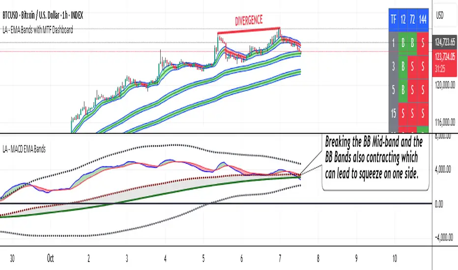
Swing Guardrail — 30-sec Midterm Check (EBITDA Margin & EV/EBITDWhat it does
Before a short-term swing entry, this indicator right-sizes positions by a quick midterm (3–12m) durability screen using two fundamentals:
EBITDA Margin (TTM) → earning power / operational resilience
EV/EBITDA (TTM) → price tag vs earning capacity (payback feel)
A high-contrast table (top-right) shows both metrics and a verdict:
PASS — both meet thresholds → normal size
HALF — only one meets → reduce size
FAIL — neither meets → avoid
Why check “midterm” for a short-term trade?
Short swings still face earnings/news gaps, failed breakouts, and regime shifts. Names with weak margins or stretched valuation tend to break faster and deeper. A 30-sec durability check helps you:
Filter fragile setups (avoid expensive + weakening names)
Stabilize drawdowns (size down when quality/price don’t align)
Keep timing unchanged while improving risk-adjusted returns
Inputs (defaults)
Min EBITDA Margin % (TTM): 8%
Max EV/EBITDA (TTM): 12
Dark chart? High-contrast colors
How to use with a swing system
Get your entry from price/volume (e.g., Ichimoku cloud break, Kijun reclaim, Tenkan>Kijun; or your A/B/C rules).
Run this check only to set size (not timing).
Optional alerts: Once per bar close for PASS / HALF / FAIL.
Size mapping & event guard
PASS → 100% of your planned size
HALF → ~50% size / tighter stops
FAIL → watchlist only
If earnings < ~10 JP business days, drop one tier; ≤3 days → avoid.
Sector guides (tweak as needed)
Software/Internet: Margin ≥ 15%, EV/EBITDA ≤ 18
Industrials/Consumer: Margin ≥ 8%, EV/EBITDA ≤ 12
Retail: Margin ≥ 5–7%, EV/EBITDA ≤ 10–12
Edge cases / substitutions
Banks/Insurers/REITs or net-cash/negative EBITDA: EV/EBITDA may mislead → consider Net Debt/EBITDA or sector metrics (CET1/LTV/DSCR).
Sparse data / fresh listings: numbers may be NA until updates.
Notes & limitations
Data via request.financial() (TTM/most-recent). Some tickers/regions can show NA until fundamentals refresh.
This is a risk-screen / sizing tool, not a buy/sell signal.
Disclaimer
Educational use only. Not investment advice.
日本語
タイトル
スイング用ガードレール―中期“壊れにくさ”30秒チェック(EBITDAマージン & EV/EBITDA, TTM)
概要
短期スイングのエントリー前に、中期(3〜12か月)の耐久性を2指標で素早く確認し、ポジションサイズを決めるためのツールです。
EBITDAマージン(TTM):事業の稼ぐ力・体力
EV/EBITDA(TTM):その体力に対する“値札”(回収年数の感覚)
右上の高コントラスト表に数値と判定を表示:
PASS:両方クリア → 通常サイズ
HALF:片方のみ → サイズ半分
FAIL:両方NG → 見送り
なぜ短期でも“中期”を確認?
短期でも決算・ニュースのギャップ、ブレイク失敗、地合い転換は起きます。マージンが弱い/割高すぎる銘柄は崩れやすく、戻りも鈍い傾向。30秒の耐久性チェックで
脆いセットアップを回避
ドローダウンを平準化(サイズで吸収)
タイミングは変えずに、リスク調整後リターンの改善を狙えます。
入力(既定)
最低EBITDAマージン:8%
最大EV/EBITDA:12
黒背景向け:高コントラスト表示
使い方(スイング手法と併用)
まずは価格シグナル(一目の雲上抜け/基準線回復/転換線>基準線、またはA/B/Cルール)。
本インジの判定でサイズのみ決定(エントリーのタイミングは出しません)。
任意でバー確定アラート(PASS/HALF/FAIL)を設定。
サイズ目安 & イベント抑制
PASS:計画サイズ100%
HALF:約50%(ストップもタイトに)
FAIL:見送り
決算まで≦10営業日なら1段階サイズダウン、≦3営業日は原則見送り。
セクター目安(調整推奨)
ソフト/ネット:マージン 15%以上、EV/EBITDA 18以下
工業/一般消費:マージン 8%以上、EV/EBITDA 12以下
小売:マージン 5〜7%以上、EV/EBITDA 10〜12以下
例外・代替
銀行・保険・REIT/ネットキャッシュ・EBITDAマイナス:EV/EBITDAは適さない場合 → Net Debt/EBITDAやCET1/LTV/DSCR等で補助。
新規上場・データ薄:更新までNAのことあり。
注意
データは request.financial() を使用。更新前はNAの可能性。
本ツールはリスク確認/サイズ調整用で、売買シグナルではありません。
免責
情報提供のみ。投資判断は自己責任で。
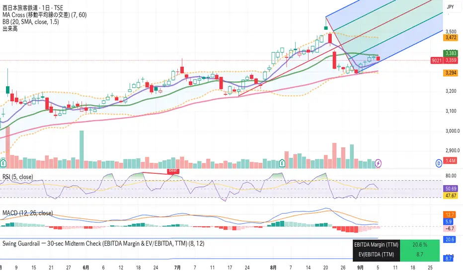
FUMO 200 MagnetWhat it does
FUMO Magnet measures how far price has stretched away from its long-term “magnet” — a blended EMA/SMA moving average (200 by default).
It plots a logarithmic deviation (optionally normalized) as an oscillator around zero.
Above 0** → price is above the magnet (stretched up)
Below 0** → price is below the magnet (stretched down)
Guide levels** highlight potential overbought/oversold zones
---
Why log deviation?
Log returns make extremes comparable across cycles and compress exponential trends — especially useful for BTC and other crypto assets.
Normalization modes further adjust the scale, keeping the oscillator readable on any chart.
---
Inputs
**Base**
* Source (default: Close)
* Base Length (default: 200 EMA/SMA)
* EMA vs SMA weight (%) — 0% = pure SMA, 100% = pure EMA, 50% = blended
* EMA smoothing of deviation — acts as a noise filter
**Normalization**
* None (Log Deviation) — raw log stretch in % terms
* Z-score — deviation in standard deviations (σ)
* Robust Z (MAD) — deviation vs median absolute deviation, resistant to outliers
* Tanh squash — smooth nonlinear squash of extremes for compact scale
* Normalization window (for Z / MAD)
* Tanh scale (lower = stronger squash)
* Clamp after normalization — hard cap at ±X
**Levels**
* Guide levels (Upper / Lower) — visual thresholds (default ±12)
* Zero line toggle
---
### How to read it
* **Trend bias**: sustained time above 0 = uptrend, below 0 = downtrend
* **Stretch / mean reversion**: the farther from 0, the higher the reversion risk
* **Cross-checks**: combine with structure (HH/HL, LH/LL), volume, or momentum (RSI, MACD)
---
### Recommended settings by timeframe
**Long-term (1D / 1W)**
* Normalization: None (Log Deviation)
* Base Length: 200
* EMA vs SMA weight: 50% (adjust 35–65% for faster/slower magnet)
* Deviation smoothing: 20 (10–30 range)
* Guide levels: ±12 to ±20
* Use case: cycle extremes, portfolio rebalancing, trim/add logic
**Swing (4H – 1D)**
* Normalization: Z-score
* Window: 200 (100–250)
* Smoothing: 14–20
* Guide levels: ±2σ to ±3σ
* Use case: stretched conditions across regimes; ±3σ is rare, often mean-reverts
**Intraday / Active swing (1H – 4H)**
* Normalization: Robust Z (MAD)
* Window: 200 (150 for faster response)
* Smoothing: 10–16
* Guide levels: ±3 to ±4 (robust units)
* Use case: handles spikes better than σ, fewer false overbought/oversold signals
**Scalping / Universal readability (15m – 1H)**
* Normalization: Tanh squash
* Tanh scale: 6–10 (start with 8)
* Smoothing: 8–12
* Guide levels: ±8 to ±12
* Use case: compact panel across assets and timeframes; not % or σ, but visually consistent
---
### Optional
* Clamp: enable ±20 (or ±25) for strict bounded range (useful for public charts)
---
### Quick setups
**BTC Daily (“cycle view”)**
* Normalization: None
* Blend: 50%
* Smooth: 20
* Levels: ±12–15
**BTC 4H (“swing”)**
* Normalization: Z-score
* Window: 200
* Smooth: 16
* Levels: ±2.5σ to ±3σ
**Alts 1H (“volatile”)**
* Normalization: Robust Z (MAD)
* Window: 200
* Smooth: 12
* Levels: ±3.5 to ±4.5
**Mixed assets 15m (“compact panel”)**
* Normalization: Tanh squash
* Scale: 8
* Smooth: 10
* Levels: ±8–12
* Clamp: ±20
Meta-LR ForecastThis indicator builds a forward-looking projection from the current bar by combining twelve time-compressed “mini forecasts.” Each forecast is a linear-regression-based outlook whose contribution is adaptively scaled by trend strength (via ADX) and normalized to each timeframe’s own volatility (via that timeframe’s ATR). The result is a 12-segment polyline that starts at the current price and extends one bar at a time into the future (1× through 12× the chart’s timeframe). Alongside the plotted path, the script computes two summary measures:
* Per-TF Bias% — a directional efficiency × R² score for each micro-forecast, expressed as a percent.
* Meta Bias% — the same score, but applied to the final, accumulated 12-step path. It summarizes how coherent and directional the combined projection is.
This tool is an indicator, not a strategy. It does not place orders. Nothing here is trade advice; it is a visual, quantitative framework to help you assess directional bias and trend context across a ladder of timeframe multiples.
The core engine fits a simple least-squares line on a normalized price series for each small forecast horizon and extrapolates one bar forward. That “trend” forecast is paired with its mirror, an “anti-trend” forecast, constructed around the current normalized price. The model then blends between these two wings according to current trend strength as measured by ADX.
ADX is transformed into a weight (w) in using an adaptive band centered on the rolling mean (μ) with width derived from the standard deviation (σ) of ADX over a configurable lookback. When ADX is deeply below the lower band, the weight approaches -1, favoring anti-trend behavior. Inside the flat band, the weight is near zero, producing neutral behavior. Clearly above the upper band, the weight approaches +1, favoring a trend-following stance. The transitions between these regions are linear so the regime shift is smooth rather than abrupt.
You can shape how quickly the model commits to either wing using two exponents. One exponent controls how aggressively positive weights lean into the trend forecast; the other controls how aggressively negative weights lean into the anti-trend forecast. Raising these exponents makes the response more gradual; lowering them makes the shift more decisive. An optional switch can force full anti-trend behavior when ADX registers a deep-low condition far below the lower tail, if you prefer a categorical stance in very flat markets.
A key design choice is volatility normalization. Every micro-forecast is computed in ATR units of its own timeframe. The script fetches that timeframe’s ATR inside each security call and converts normalized outputs back to price with that exact ATR. This avoids scaling higher-timeframe effects by the chart ATR or by square-root time approximations. Using “ATR-true” for each timeframe keeps the cross-timeframe accumulation consistent and dimensionally correct.
Bias% is defined as directional efficiency multiplied by R², expressed as a percent. Directional efficiency captures how much net progress occurred relative to the total path length; R² captures how well the path aligns with a straight line. If price meanders without net progress, efficiency drops; if the variation is well-explained by a line, R² rises. Multiplying the two penalizes choppy, low-signal paths and rewards sustained, coherent motion.
The forward path is built by converting each per-timeframe Bias% into a small ATR-sized delta, then cumulatively adding those deltas to form a 12-step projection. This produces a polyline anchored at the current close and stepping forward one bar per timeframe multiple. Segment color flips by slope, allowing a quick read of the path’s direction and inflection.
Inputs you can tune include:
* Max Regression Length. Upper bound for each micro-forecast’s regression window. Larger values smooth the trend estimate at the cost of responsiveness; smaller values react faster but can add noise.
* Price Source. The price series analyzed (for example, close or typical price).
* ADX Length. Period used for the DMI/ADX calculation.
* ATR Length (normalization). Window used for ATR; this is applied per timeframe inside each security call.
* Band Lookback (for μ, σ). Lookback used to compute the adaptive ADX band statistics. Larger values stabilize the band; smaller values react more quickly.
* Flat half-width (σ). Width of the neutral band on both sides of μ. Wider flats spend more time neutral; narrower flats switch regimes more readily.
* Tail width beyond flat (σ). Distance from the flat band edge to the extreme trend/anti-trend zone. Larger tails create a longer ramp; smaller tails reach extremes sooner.
* Polyline Width. Visual thickness of the plotted segments.
* Negative Wing Aggression (anti-trend). Exponent shaping for negative weights; higher values soften the tilt into mean reversion.
* Positive Wing Aggression (trend). Exponent shaping for positive weights; lower values make trend commitment stronger and sooner.
* Force FULL Anti-Trend at Deep-Low ADX. Optional hard switch for extremely low ADX conditions.
On the chart you will see:
* A 12-segment forward polyline starting from the current close to bar\_index + 1 … +12, with green segments for up-steps and red for down-steps.
* A small label at the latest bar showing Meta Bias% when available, or “n/a” when insufficient data exists.
Interpreting the readouts:
* Trend-following contexts are characterized by ADX above the adaptive upper band, pushing w toward +1. The blended forecast leans toward the regression extrapolation. A strongly positive Meta Bias% in this environment suggests directional alignment across the ladder of timeframes.
* Mean-reversion contexts occur when ADX is well below the lower tail, pushing w toward -1 (or forcing anti-trend if enabled). After a sharp advance, a negative Meta Bias% may indicate the model projects pullback tendencies.
* Neutral contexts occur when ADX sits inside the flat band; w is near zero, the blended forecast remains close to current price, and Meta Bias% tends to hover near zero.
These are analytical cues, not rules. Always corroborate with your broader process, including market structure, time-of-day behavior, liquidity conditions, and risk limits.
Practical usage patterns include:
* Momentum confirmation. Combine a rising Meta Bias% with higher-timeframe structure (such as higher highs and higher lows) to validate continuation setups. Treat the 12th step’s distance as a coarse sense of potential room rather than as a target.
* Fade filtering. If you prefer fading extremes, require ADX to be near or below the lower ramp before acting on counter-moves, and avoid fades when ADX is decisively above the upper band.
* Position planning. Because per-step deltas are ATR-scaled, the path’s vertical extent can be mentally mapped to typical noise for the instrument, informing stop distance choices. The script itself does not compute orders or size.
* Multi-timeframe alignment. Each step corresponds to a clean multiple of your chart timeframe, so the polyline visualizes how successively larger windows bias price, all referenced to the current bar.
House-rules and repainting disclosures:
* Indicator, not strategy. The script does not execute, manage, or suggest orders. It displays computed paths and bias scores for analysis only.
* No performance claims. Past behavior of any measure, including Meta Bias%, does not guarantee future results. There are no assurances of profitability.
* Higher-timeframe updates. Values obtained via security for higher-timeframe series can update intrabar until the higher-timeframe bar closes. The forward path and Meta Bias% may change during formation of a higher-timeframe candle. If you need confirmed higher-timeframe inputs, consider reading the prior higher-timeframe value or acting only after the higher-timeframe close.
* Data sufficiency. The model requires enough history to compute ATR, ADX statistics, and regression windows. On very young charts or illiquid symbols, parts of the readout can be unavailable until sufficient data accumulates.
* Volatility regimes. ATR normalization helps compare across timeframes, but unusual volatility regimes can make the path look deceptively flat or exaggerated. Judge the vertical scale relative to your instrument’s typical ATR.
Tuning tips:
* Stability versus responsiveness. Increase Max Regression Length to steady the micro-forecasts but accept slower response. If you lower it, consider slightly increasing Band Lookback so regime boundaries are not too jumpy.
* Regime bands. Widen the flat half-width to spend more time neutral, which can reduce over-trading tendencies in chop. Shrink the tail width if you want the model to commit to extremes sooner, at the cost of more false swings.
* Wing shaping. If anti-trend behavior feels too abrupt at low ADX, raise the negative wing exponent. If you want trend bias to kick in more decisively at high ADX, lower the positive wing exponent. Small changes have large effects.
* Forced anti-trend. Enable the deep-low option only if you explicitly want a categorical “markets are flat, fade moves” policy. Many users prefer leaving it off to keep regime decisions continuous.
Troubleshooting:
* Nothing plots or the label shows “n/a.” Ensure the chart has enough history for the ADX band statistics, ATR, and the regression windows. Exotic or illiquid symbols with missing data may starve the higher-timeframe computations. Try a more liquid market or a higher timeframe.
* Path flickers or shifts during the bar. This is expected when any higher-timeframe input is still forming. Wait for the higher-timeframe close for fully confirmed behavior, or modify the code to read prior values from the higher timeframe.
* Polyline looks too flat or too steep. Check the chart’s vertical scale and recent ATR regime. Adjust Max Regression Length, the wing exponents, or the band widths to suit the instrument.
Integration ideas for manual workflows:
* Confluence checklist. Use Meta Bias% as one of several independent checks, alongside structure, session context, and event risk. Act only when multiple cues align.
* Stop and target thinking. Because deltas are ATR-scaled at each timeframe, benchmark your proposed stops and targets against the forward steps’ magnitude. Stops that are much tighter than the prevailing ATR often sit inside normal noise.
* Session context. Consider session hours and microstructure. The same ADX value can imply different tradeability in different sessions, particularly in index futures and FX.
This indicator deliberately avoids:
* Fixed thresholds for buy or sell decisions. Markets vary and fixed numbers invite overfitting. Decide what constitutes “high enough” Meta Bias% for your market and timeframe.
* Automatic risk sizing. Proper sizing depends on account parameters, instrument specifications, and personal risk tolerance. Keep that decision in your risk plan, not in a visual bias tool.
* Claims of edge. These measures summarize path geometry and trend context; they do not ensure a tradable edge on their own.
Summary of how to think about the output:
* The script builds a 12-step forward path by stacking linear-regression micro-forecasts across increasing multiples of the chart timeframe.
* Each micro-forecast is blended between trend and anti-trend using an adaptive ADX band with separate aggression controls for positive and negative regimes.
* All computations are done in ATR-true units for each timeframe before reconversion to price, ensuring dimensional consistency when accumulating steps.
* Bias% (per-timeframe and Meta) condenses directional efficiency and trend fidelity into a compact score.
* The output is designed to serve as an analytical overlay that helps assess whether conditions look trend-friendly, fade-friendly, or neutral, while acknowledging higher-timeframe update behavior and avoiding prescriptive trade rules.
Use this tool as one component within a disciplined process that includes independent confirmation, event awareness, and robust risk management.

CDC ActionZone BF for ETHUSD-1D © PRoSkYNeT-EE
Based on improvements from "Kitti-Playbook Action Zone V.4.2.0.3 for Stock Market"
Based on improvements from "CDC Action Zone V3 2020 by piriya33"
Based on Triple MACD crossover between 9/15, 21/28, 15/28 for filter error signal (noise) from CDC ActionZone V3
MACDs generated from the execution of millions of times in the "Brute Force Algorithm" to backtest data from the past 5 years. ( 2017-08-21 to 2022-08-01 )
Released 2022-08-01
***** The indicator is used in the ETHUSD 1 Day period ONLY *****
Recommended Stop Loss : -4 % (execute stop Loss after candlestick has been closed)
Backtest Result ( Start $100 )
Winrate 63 % (Win:12, Loss:7, Total:19)
Live Days 1,806 days
B : Buy
S : Sell
SL : Stop Loss
2022-07-19 07 - 1,542 : B 6.971 ETH
2022-04-13 07 - 3,118 : S 8.98 % $10,750 12,7,19 63 %
2022-03-20 07 - 2,861 : B 3.448 ETH
2021-12-03 07 - 4,216 : SL -8.94 % $9,864 11,7,18 61 %
2021-11-30 07 - 4,630 : B 2.340 ETH
2021-11-18 07 - 3,997 : S 13.71 % $10,832 11,6,17 65 %
2021-10-05 07 - 3,515 : B 2.710 ETH
2021-09-20 07 - 2,977 : S 29.38 % $9,526 10,6,16 63 %
2021-07-28 07 - 2,301 : B 3.200 ETH
2021-05-20 07 - 2,769 : S 50.49 % $7,363 9,6,15 60 %
2021-03-30 07 - 1,840 : B 2.659 ETH
2021-03-22 07 - 1,681 : SL -8.29 % $4,893 8,6,14 57 %
2021-03-08 07 - 1,833 : B 2.911 ETH
2021-02-26 07 - 1,445 : S 279.27 % $5,335 8,5,13 62 %
2020-10-13 07 - 381 : B 3.692 ETH
2020-09-05 07 - 335 : S 38.43 % $1,407 7,5,12 58 %
2020-07-06 07 - 242 : B 4.199 ETH
2020-06-27 07 - 221 : S 28.49 % $1,016 6,5,11 55 %
2020-04-16 07 - 172 : B 4.598 ETH
2020-02-29 07 - 217 : S 47.62 % $791 5,5,10 50 %
2020-01-12 07 - 147 : B 3.644 ETH
2019-11-18 07 - 178 : S -2.73 % $536 4,5,9 44 %
2019-11-01 07 - 183 : B 3.010 ETH
2019-09-23 07 - 201 : SL -4.29 % $551 4,4,8 50 %
2019-09-18 07 - 210 : B 2.740 ETH
2019-07-12 07 - 275 : S 63.69 % $575 4,3,7 57 %
2019-05-03 07 - 168 : B 2.093 ETH
2019-04-28 07 - 158 : S 29.51 % $352 3,3,6 50 %
2019-02-15 07 - 122 : B 2.225 ETH
2019-01-10 07 - 125 : SL -6.02 % $271 2,3,5 40 %
2018-12-29 07 - 133 : B 2.172 ETH
2018-05-22 07 - 641 : S 5.95 % $289 2,2,4 50 %
2018-04-21 07 - 605 : B 0.451 ETH
2018-02-02 07 - 922 : S 197.42 % $273 1,2,3 33 %
2017-11-11 07 - 310 : B 0.296 ETH
2017-10-09 07 - 297 : SL -4.50 % $92 0,2,2 0 %
2017-10-07 07 - 311 : B 0.309 ETH
2017-08-22 07 - 310 : SL -4.02 % $96 0,1,1 0 %
2017-08-21 07 - 323 : B 0.310 ETH
Bar Balance [LucF]Bar Balance extracts the number of up, down and neutral intrabars contained in each chart bar, revealing information on the strength of price movement. It can display stacked columns representing raw up/down/neutral intrabar counts, or an up/down balance line which can be calculated and visualized in many different ways.
WARNING: This is an analysis tool that works on historical bars only. It does not show any realtime information, and thus cannot be used to issue alerts or for automated trading. When realtime bars elapse, the indicator will require a browser refresh, a change to its Inputs or to the chart's timeframe/symbol to recalculate and display information on those elapsed bars. Once a trader understands this, the indicator can be used advantageously to make discretionary trading decisions.
Traders used to work with my Delta Volume Columns Pro will feel right at home in this indicator's Inputs . It has lots of options, allowing it to be used in many different ways. If you value the bar balance information this indicator mines, I hope you will find the time required to master the use of Bar Balance well worth the investment.
█ OVERVIEW
The indicator has two modes: Columns and Line .
Columns
• In Columns mode you can display stacked Up/Down/Neutral columns.
• The "Up" section represents the count of intrabars where `close > open`, "Down" where `close < open` and "Neutral" where `close = open`.
• The Up section always appears above the centerline, the Down section below. The Neutral section overlaps the centerline, split halfway above and below it.
The Up and Down sections start where the Neutral section ends, when there is one.
• The Up and Down sections can be colored independently using 7 different methods.
• The signal line plotted in Line mode can also be displayed in Columns mode.
Line
• Displays a single balance line using a zero centerline.
• A variable number of independent methods can be used to calculate the line (6), determine its color (5), and color the fill (5).
You can thus evaluate the state of 3 different components with this single line.
• A "Divergence Levels" feature will use the line to automatically draw expanding levels on divergence events.
Features available in both modes
• The color of all components can be selected from 15 base colors, with 16 gradient levels used for each base color in the indicator's gradients.
• A zero line can show a 6-state aggregate value of the three main volume balance modes.
• The background can be colored using any of 5 different methods.
• Chart bars can be colored using 5 different methods.
• Divergence and large neutral count ratio events can be shown in either Columns or Line mode, calculated in one of 4 different methods.
• Markers on 6 different conditions can be displayed.
█ CONCEPTS
Intrabar inspection
Intrabar inspection means the indicator looks at lower timeframe bars ( intrabars ) making up a given chart bar to gather its information. If your chart is on a 1-hour timeframe and the intrabar resolution determined by the indicator is 5 minutes, then 12 intrabars will be analyzed for each chart bar and the count of up/down/neutral intrabars among those will be tallied.
Bar Balances and calculation methods
The indicator uses a variety of methods to evaluate bar balance and to derive other calculations from them:
1. Balance on Bar : Uses the relative importance of instant Up and Down counts on the bar.
2. Balance Averages : Uses the difference between the EMAs of Up and Down counts.
3. Balance Momentum : Starts by calculating, separately for both Up and Down counts, the difference between the same EMAs used in Balance Averages and an SMA of double the period used for the EMAs. These differences are then aggregated and finally, a bounded momentum of that aggregate is calculated using RSI.
4. Markers Bias : It sums the bull/bear occurrences of the four previous markers over a user-defined period (the default is 14).
5. Combined Balances : This is the aggregate of the instant bull/bear bias of the three main bar balances.
6. Dual Up/Down Averages : This is a display mode showing the EMA calculated for each of the Up and Down counts.
Interpretation of neutral intrabars
What do neutral intrabars mean? When price does not change during a bar, it can be because there is simply no interest in the market, or because of a perfect balance between buyers and sellers. The latter being more improbable, Bar Balance assumes that neutral bars reveal a lack of interest, which entails uncertainty. That is the reason why the option is provided to interpret ratios of neutral intrabars greater than 50% as divergences. It is also the rationale behind the option to dampen signal lines on the inverse ratio of neutral intrabars, so that zero intrabars do not affect the signal, and progressively larger proportions of neutral intrabars will reduce the signal's amplitude, as the balance calcs using the up/down counts lose significance. The impact of the dampening will vary with markets. Weaker markets such as cryptos will often contain greater numbers of neutral intrabars, so dampening the Line in that sector will have a greater impact than in more liquid markets.
█ FEATURES
1 — Columns
• While the size of the Up/Down columns always represents their respective importance on the bar, their coloring mode is independent. The default setup uses a standard coloring mode where the Up/Down columns over/under the zero line are always in the bull/bear color with a higher intensity for the winning side. Six other coloring modes allow you to pack more information in the columns. When choosing to color the top columns using a bull/bear gradient on Balance Averages, for example, you will end up with bull/bear colored tops. In order for the color of the bottom columns to continue to show the instant bar balance, you can then choose the "Up/Down Ratio on Bar — Dual Solid Colors" coloring mode to make those bars the color of the winning side for that bar.
• Line mode shows only the line, but Columns mode allows displaying the line along with it. If the scale of the line is different than that of the scale of the columns, the line will often appear flat. Traders may find even a flat line useful as its bull/bear colors will be easily distinguishable.
2 — Line
• The default setup for Line mode uses a calculation on "Balance Momentum", with a fill on the longer-term "Balance Averages" and a line color based on the "Markers Bias". With the background set on "Line vs Divergence Levels" and the zero line on the hard-coded "Combined Bar Balances", you have access to five distinct sources of information at a glance, to which you can add divergences, divergences levels and chart bar coloring. This provides powerful potential in displaying bar balance information.
• When no columns are displayed, Line mode can show the full scale of whichever line you choose to calculate because the columns' scale no longer interferes with the line's scale.
• Note that when "Balance on Bar" is selected, the Neutral count is also displayed as a ratio of the balance line. This is the only instance where the Neutral count is displayed in Line mode.
• The "Dual Up/Down Averages" is an exception as it displays two lines: one average for the Up counts and another for the Down counts. This mode will be most useful when Columns are also displayed, as it provides a reference for the top and bottom columns.
3 — Zero Line
The zero line can be colored using two methods, both based on the Combined Balances, i.e., the aggregate of the instant bull/bear bias of the three main bar balances.
• In "Six-state Dual Color Gradient" mode, a dot appears on every bar. Its color reflects the bull/bear state of the Combined Balances, and the dot's brightness reflects the tally of balance biases.
• In "Dual Solid Colors (All Bull/All Bear Only)" a dot only appears when all three balances are either bullish or bearish. The resulting pattern is identical to that of Marker 1.
4 — Divergences
• Divergences are displayed as a small circle at the top of the scale. Four different types of divergence events can be detected. Divergences occur whenever the bull/bear bias of the method used diverges with the bar's price direction.
• An option allows you to include in divergence events instances where the count of neutral intrabars exceeds 50% of the total intrabar count.
• The divergence levels are dynamic levels that automatically build from the line's values on divergence events. On consecutive divergences, the levels will expand, creating a channel. This implementation of the divergence levels corresponds to my view that divergences indicate anomalies, hesitations, points of uncertainty if you will. It excludes any association of a pre-determined bullish/bearish bias to divergences. Accordingly, the levels merely take note of divergence events and mark those points in time with levels. Traders then have a reference point from which they can evaluate further movement. The bull/bear/neutral colors used to plot the levels are also congruent with this view in that they are determined by price's position relative to the levels, which is how I think divergences can be put to the most effective use.
5 — Background
• The background can show a bull/bear gradient on four different calculations. You can adjust its brightness to make its visual importance proportional to how you use it in your analysis.
6 — Chart bars
• Chart bars can be colored using five different methods.
• You have the option of emptying the body of bars where volume does not increase, as does my TLD indicator, the idea behind this being that movement on bars where volume does not increase is less relevant.
7 — Intrabar Resolution
You can choose between three modes. Two of them are automatic and one is manual:
a) Fast, Longer history, Auto-Steps (~12 intrabars) : Optimized for speed and deeper history. Uses an average minimum of 12 intrabars.
b) More Precise, Shorter History Auto-Steps (~24 intrabars) : Uses finer intrabar resolution. It is slower and provides less history. Uses an average minimum of 24 intrabars.
c) Fixed : Uses the fixed resolution of your choice.
Auto-Steps calculations vary for 24/7 and conventional markets in order to achieve the proper target of minimum intrabars.
You can choose to view the intrabar resolution currently used to calculate delta volume. It is the default.
The proper selection of the intrabar resolution is important. It must achieve maximal granularity to produce precise results while not unduly slowing down calculations, or worse, causing runtime errors.
8 — Markers
Six markers are available:
1. Combined Balances Agreement : All three Bar Balances are either bullish or bearish.
2. Up or Down % Agrees With Bar : An up marker will appear when the percentage of up intrabars in an up chart bar is greater than the specified percentage. Conditions mirror to down bars.
3. Divergence confirmations By Price : One of the four types of balance calculations can be used to detect divergences with price. Confirmations occur when the bar following the divergence confirms the balance bias. Note that the divergence events used here do not include neutral intrabar events.
4. Balance Transitions : Bull/bear transitions of the selected balance.
5. Markers Bias Transitions : Bull/bear transitions of the Markers Bias.
6. Divergence Confirmations By Line : Marks points where the line first breaches a divergence level.
Markers appear when the condition is detected, without delay. Since nothing is plotted in realtime, markers do not appear on the realtime bar.
9 — Settings
• Two modes can be selected to dampen the line on the ratio of neutral intrabars.
• A distinct weight can be attributed to the count of the latter half of intrabars, on the assumption that later intrabars may be more important in determining the outcome of chart bars.
• Allows control over the periods of the different moving averages used in calculations.
• The default periods used for the various calculations define the following hierarchy from slow to fast:
Balance Averages: 50,
Balance Momentum: 20,
Dual Up/Down Averages: 20,
Marker Bias: 10.
█ LIMITATIONS
• This script uses a special characteristic of the `security()` function allowing the inspection of intrabars—which is not officially supported by TradingView.
• The method used does not work on the realtime bar—only on historical bars.
• The indicator only works on some chart resolutions: 3, 5, 10, 15 and 30 minutes, 1, 2, 4, 6, and 12 hours, 1 day, 1 week and 1 month. The script’s code can be modified to run on other resolutions, but chart resolutions must be divisible by the lower resolution used for intrabars and the stepping mechanism could require adaptation.
• When using the "Line vs Divergence Levels — Dual Color Gradient" color mode to fill the line, background or chart bars, keep in mind that a line calculation mode must be defined for it to work, as it determines gradients on the movement of the line relative to divergence levels. If the line is hidden, it will not work.
• When the difference between the chart’s resolution and the intrabar resolution is too great, runtime errors will occur. The Auto-Steps selection mechanisms should avoid this.
• Alerts do not work reliably when `security()` is used at intrabar resolutions. Accordingly, no alerts are configured in the indicator.
• The color model used in the indicator provides for fancy visuals that come at a price; when you change values in Inputs , it can take 20 seconds for the changes to materialize. Luckily, once your color setup is complete, the color model does not have a large performance impact, as in normal operation the `security()` calls will become the most important factor in determining response time. Also, once in a while a runtime error will occur when you change inputs. Just making another change will usually bring the indicator back up.
█ RAMBLINGS
Is this thing useful?
I'll let you decide. Bar Balance acts somewhat like an X-Ray on bars. The intrabars it analyzes are no secret; one can simply change the chart's resolution to see the same intrabars the indicator uses. What the indicator brings to traders is the precise count of up/down/neutral intrabars and, more importantly, the calculations it derives from them to present the information in a way that can make it easier to use in trading decisions.
How reliable is Bar Balance information?
By the same token that an up bar does not guarantee that more up bars will follow, future price movements cannot be inferred from the mere count of up/down/neutral intrabars. Price movement during any chart bar for which, let's say, 12 intrabars are analyzed, could be due to only one of those intrabars. One can thus easily see how only relying on bar balance information could be very misleading. The rationale behind Bar Balance is that when the information mined for multiple chart bars is aggregated, it can provide insight into the history behind chart bars, and thus some bias as to the strength of movements. An up chart bar where 11/12 intrabars are also up is assumed to be stronger than the same up bar where only 2/12 intrabars are up. This logic is not bulletproof, and sometimes Bar Balance will stray. Also, keep in mind that balance lines do not represent price momentum as RSI would. Bar Balance calculations have no idea where price is. Their perspective, like that of any historian, is very limited, constrained that it is to the narrow universe of up/down/neutral intrabar counts. You will thus see instances where price is moving up while Balance Momentum, for example, is moving down. When Bar Balance performs as intended, this indicates that the rally is weakening, which does necessarily imply that price will reverse. Occasionally, price will merrily continue to advance on weakening strength.
Divergences
Most of the divergence detection methods used here rely on a difference between the bias of a calculation involving a multi-bar average and a given bar's price direction. When using "Bar Balance on Bar" however, only the bar's balance and price movement are used. This is the default mode.
As usual, divergences are points of interest because they reveal imbalances, which may or may not become turning points. I do not share the overwhelming enthusiasm traders have for the purported ability of bullish/bearish divergences to indicate imminent reversals.
Superfluity
In "The Bed of Procrustes", Nassim Nicholas Taleb writes: To bankrupt a fool, give him information . Bar Balance can display lots of information. While learning to use a new indicator inevitably requires an adaptation period where we put it through its paces and try out all its options, once you have become used to Bar Balance and decide to adopt it, rigorously eliminate the components you don't use and configure the remaining ones so their visual prominence reflects their relative importance in your analysis. I tried to provide flexible options for traders to control this indicator's visuals for that exact reason—not for window dressing.
█ NOTES
For traders
• To avoid misleading traders who don't read script descriptions, the indicator shows nothing in the realtime bar.
• The Data Window shows key values for the indicator.
• All gradients used in this indicator determine their brightness intensities using advances/declines in the signal—not their relative position in a fixed scale.
• Note that because of the way gradients are optimized internally, changing their brightness will sometimes require bringing down the value a few steps before you see an impact.
• Because this indicator does not use volume, it will work on all markets.
For coders
• For those interested in gradients, this script uses an advanced version of the Advance/Decline gradient function from the PineCoders Color Gradient (16 colors) Framework . It allows more precise control over the range, steps and min/max values of the gradients.
• I use the PineCoders Coding Conventions for Pine to write my scripts.
• I used functions modified from the PineCoders MTF Selection Framework for the selection of timeframes.
█ THANKS TO:
— alexgrover who helped me think through the dampening method used to attenuate signal lines on high ratios of neutral intrabars.
— A guy called Kuan who commented on a Backtest Rookies presentation of their Volume Profile indicator . The technique I use to inspect intrabars is derived from Kuan's code.
— theheirophant , my partner in the exploration of the sometimes weird abysses of `security()`’s behavior at intrabar resolutions.
— midtownsk8rguy , my brilliant companion in mining the depths of Pine graphics. He is also the co-author of the PineCoders Color Gradient Frameworks .

12M Return Strategy This strategy is based on the original Dual Momentum concept presented by Gary Antonacci in his book “Dual Momentum Investing.”
It implements the absolute momentum portion of the framework using a 12-month rate of change, combined with a moving-average filter for trend confirmation.
The script automatically adapts the lookback period depending on chart timeframe, ensuring the return calculation always represents approximately one year, whether you are on daily, weekly, or monthly charts.
How the Strategy Works
1. 12-Month Return Calculation
The core signal is the 12-month price return, computed as:
(Current Price ÷ Price from ~1 year ago) − 1
This return:
Plots as a histogram
Turns green when positive
Turns red when negative
The lookback adjusts automatically:
1D chart → 252 bars
1W chart → 52 bars
1M chart → 12 bars
Other timeframes → estimated to approximate 1 calendar year
2. Trend Filter (Moving Average of Return)
To smooth volatility and avoid noise, the strategy applies a moving average to the 12M return:
Default length: 12 periods
Plotted as a white line on the indicator panel
This becomes the benchmark used for crossovers.
3. Trade Signals (Long / Short / Cash)
Trades are generated using a simple crossover mechanism:
Bullish Signal (Go Long)
When:
12M Return crosses ABOVE its MA
Action:
Close short (if any)
Enter long
Bearish Signal (Go Short or Go Flat)
When:
12M Return crosses BELOW its MA
Action:
If shorting is enabled → Enter short
If shorting is disabled → Exit position and go to cash
Shorting can be enabled or disabled with a single input switch.
4. Position Sizing
The strategy uses:
Percent of Equity position sizing
You can specify the percentage of your portfolio to allocate (default 100%).
No leverage is required, but the strategy supports it if your account settings allow.
5. Visual Signals
To improve clarity, the strategy marks signals directly on the indicator panel:
Green Up Arrows: return > MA
Red Down Arrows: return < MA
A status label shows the current mode:
LONG
SHORT
CASH
6. Backtest-Ready
This script is built as a full TradingView strategy, not just an indicator.
This means you can:
Run complete backtests
View performance metrics
Compare long-only vs long/short behavior
Adjust inputs to tune the system
It provides a clean, rule-driven interpretation of the classic absolute momentum approach.
Inspired By: Gary Antonacci – Dual Momentum Investing
This script reflects the absolute momentum side of Antonacci’s original research:
Uses 12-month momentum (the most statistically validated lookback)
Applies a trend-following overlay to control downside risk
Recreates the classic signal structure used in academic studies
It is a simplified, transparent version intended for practical use and educational clarity.
Disclaimer
This script is for educational and research purposes only.
Historical performance does not guarantee future results.
Always use proper risk management.
Static K-means Clustering | InvestorUnknownStatic K-Means Clustering is a machine-learning-driven market regime classifier designed for traders who want a data-driven structure instead of subjective indicators or manually drawn zones.
This script performs offline (static) K-means training on your chosen historical window. Using four engineered features:
RSI (Momentum)
CCI (Price deviation / Mean reversion)
CMF (Money flow / Strength)
MACD Histogram (Trend acceleration)
It groups past market conditions into K distinct clusters (regimes). After training, every new bar is assigned to the nearest cluster via Euclidean distance in 4-dimensional standardized feature space.
This allows you to create models like:
Regime-based long/short filters
Volatility phase detectors
Trend vs. chop separation
Mean-reversion vs. breakout classification
Volume-enhanced money-flow regime shifts
Full machine-learning trading systems based solely on regimes
Note:
This script is not a universal ML strategy out of the box.
The user must engineer the feature set to match their trading style and target market.
K-means is a tool, not a ready made system, this script provides the framework.
Core Idea
K-means clustering takes raw, unlabeled market observations and attempts to discover structure by grouping similar bars together.
// STEP 1 — DATA POINTS ON A COORDINATE PLANE
// We start with raw, unlabeled data scattered in 2D space (x/y).
// At this point, nothing is grouped—these are just observations.
// K-means will try to discover structure by grouping nearby points.
//
// y ↑
// |
// 12 | •
// | •
// 10 | •
// | •
// 8 | • •
// |
// 6 | •
// |
// 4 | •
// |
// 2 |______________________________________________→ x
// 2 4 6 8 10 12 14
//
//
//
// STEP 2 — RANDOMLY PLACE INITIAL CENTROIDS
// The algorithm begins by placing K centroids at random positions.
// These centroids act as the temporary “representatives” of clusters.
// Their starting positions heavily influence the first assignment step.
//
// y ↑
// |
// 12 | •
// | •
// 10 | • C2 ×
// | •
// 8 | • •
// |
// 6 | C1 × •
// |
// 4 | •
// |
// 2 |______________________________________________→ x
// 2 4 6 8 10 12 14
//
//
//
// STEP 3 — ASSIGN POINTS TO NEAREST CENTROID
// Each point is compared to all centroids.
// Using simple Euclidean distance, each point joins the cluster
// of the centroid it is closest to.
// This creates a temporary grouping of the data.
//
// (Coloring concept shown using labels)
//
// - Points closer to C1 → Cluster 1
// - Points closer to C2 → Cluster 2
//
// y ↑
// |
// 12 | 2
// | 1
// 10 | 1 C2 ×
// | 2
// 8 | 1 2
// |
// 6 | C1 × 2
// |
// 4 | 1
// |
// 2 |______________________________________________→ x
// 2 4 6 8 10 12 14
//
// (1 = assigned to Cluster 1, 2 = assigned to Cluster 2)
// At this stage, clusters are formed purely by distance.
Your chosen historical window becomes the static training dataset , and after fitting, the centroids never change again.
This makes the model:
Predictable
Repeatable
Consistent across backtests
Fast for live use (no recalculation of centroids every bar)
Static Training Window
You select a period with:
Training Start
Training End
Only bars inside this range are used to fit the K-means model. This window defines:
the market regime examples
the statistical distributions (means/std) for each feature
how the centroids will be positioned post-trainin
Bars before training = fully transparent
Training bars = gray
Post-training bars = full colored regimes
Feature Engineering (4D Input Vector)
Every bar during training becomes a 4-dimensional point:
This combination balances: momentum, volatility, mean-reversion, trend acceleration giving the algorithm a richer "market fingerprint" per bar.
Standardization
To prevent any feature from dominating due to scale differences (e.g., CMF near zero vs CCI ±200), all features are standardized:
standardize(value, mean, std) =>
(value - mean) / std
Centroid Initialization
Centroids start at diverse coordinates using various curves:
linear
sinusoidal
sign-preserving quadratic
tanh compression
init_centroids() =>
// Spread centroids across using different shapes per feature
for c = 0 to k_clusters - 1
frac = k_clusters == 1 ? 0.0 : c / (k_clusters - 1.0) // 0 → 1
v = frac * 2 - 1 // -1 → +1
array.set(cent_rsi, c, v) // linear
array.set(cent_cci, c, math.sin(v)) // sinusoidal
array.set(cent_cmf, c, v * v * (v < 0 ? -1 : 1)) // quadratic sign-preserving
array.set(cent_mac, c, tanh(v)) // compressed
This makes initial cluster spread “random” even though true randomness is hardly achieved in pinescript.
K-Means Iterative Refinement
The algorithm repeats these steps:
(A) Assignment Step, Each bar is assigned to the nearest centroid via Euclidean distance in 4D:
distance = sqrt(dx² + dy² + dz² + dw²)
(B) Update Step, Centroids update to the mean of points assigned to them. This repeats iterations times (configurable).
LIVE REGIME CLASSIFICATION
After training, each new bar is:
Standardized using the training mean/std
Compared to all centroids
Assigned to the nearest cluster
Bar color updates based on cluster
No re-training occurs. This ensures:
No lookahead bias
Clean historical testing
Stable regimes over time
CLUSTER BEHAVIOR & TRADING LOGIC
Clusters (0, 1, 2, 3…) hold no inherent meaning. The user defines what each cluster does.
Example of custom actions:
Cluster 0 → Cash
Cluster 1 → Long
Cluster 2 → Short
Cluster 3+ → Cash (noise regime)
This flexibility means:
One trader might have cluster 0 as consolidation.
Another might repurpose it as a breakout-loading zone.
A third might ignore 3 clusters entirely.
Example on ETHUSD
Important Note:
Any change of parameters or chart timeframe or ticker can cause the “order” of clusters to change
The script does NOT assume any cluster equals any actionable bias, user decides.
PERFORMANCE METRICS & ROC TABLE
The indicator computes average 1-bar ROC for each cluster in:
Training set
Test (live) set
This helps measure:
Cluster profitability consistency
Regime forward predictability
Whether a regime is noise, trend, or reversion-biased
EQUITY SIMULATION & FEES
Designed for close-to-close realistic backtesting.
Position = cluster of previous bar
Fees applied only on regime switches. Meaning:
Staying long → no fee
Switching long→short → fee applied
Switching any→cash → fee applied
Fee input is percentage, but script already converts internally.
Disclaimers
⚠️ This indicator uses machine-learning but does not predict the future. It classifies similarity to past regimes, nothing more.
⚠️ Backtest results are not indicative of future performance.
⚠️ Clusters have no inherent “bullish” or “bearish” meaning. You must interpret them based on your testing and your own feature engineering.

Monthly Color Marker V4
## 📊 Monthly Color Marker - Historical Month Highlighting
### Overview
A unique indicator that allows rapid identification of all monthly candles from a specific month across multiple years. The indicator marks candles with different colors based on their direction (bullish/bearish), enabling quick analysis of seasonal patterns and cyclical behavior of stocks or assets.
### 🎯 Purpose
- **Identify Seasonal Patterns (Seasonality)** - Discover recurring trends in specific months
- **Quick Historical Analysis** - Visual representation of monthly performance over the years
- **Direction Recognition** - Instant understanding of whether a month tends to be bullish or bearish
- **Seasonal Trading Planning** - Build strategies based on cyclical patterns
### ⚙️ Adjustable Parameters
1. **Month to Mark (1-12)**
- Select the desired month for analysis
- 1 = January, 2 = February... 12 = December
- Default: 11 (November)
2. **Years Back (1-50)**
- Determines how many years back to scan
- Recommended: 10-25 years for statistically reliable data
- Default: 25 years
3. **Bullish Candle Color**
- Color for marking bullish candles (close > open)
- Default: Green
- Customizable to your personal color scheme
4. **Bearish Candle Color**
- Color for marking bearish candles (close < open)
- Default: Red
- Customizable to your personal color scheme
5. **Show Current Year**
- Whether to include the current month in the marking
- Useful when the month hasn't finished yet
- Default: Yes
### 📈 How to Use the Indicator
#### Step 1: Adding to Chart
1. Switch to **Monthly timeframe** - Required!
2. Add the indicator to your chart
3. Select the month you want to analyze
#### Step 2: Initial Analysis
- **Count green vs red candles** - What's the ratio?
- **Look for patterns** - Are there years where the month always rises/falls?
- **Identify outliers** - Years where behavior was different
#### Step 3: Making Decisions
- **Mostly green** → Statistically, the month tends to rise
- **Mostly red** → Statistically, the month tends to fall
- **Mixed** → No clear seasonal pattern
### 💡 Usage Examples
**Example 1: "Santa Claus Rally"**
- Select month 12 (December)
- Check if there are mostly green candles
- If yes, this confirms the well-known year-end rally effect
**Example 2: "September Effect"**
- Select month 9 (September)
- Historically, September is considered a weak month
- Do the data support this for this stock?
**Example 3: Quarterly Earnings**
- Identify which month earnings are released
- Check the historical response
- Plan entry/exit accordingly
### 🔍 Combining with Other Indicators
This indicator works excellently with:
- **Historical Monthly Levels** (the first indicator) - Identify nearby price levels
- **Volume Profile** - Check volume during those months
- **RSI/MACD** - Identify momentum strength in specific months
### ⚠️ Important Notes
1. **Must use Monthly timeframe!** The indicator won't work correctly on other timeframes
2. **Statistical Sample** - More years = more reliable analysis
3. **Not a Guarantee** - Past performance doesn't guarantee future results, use additional analysis
4. **Adjust Colors** - If hard to see, change colors in settings
### 🎨 Tips for Optimal Experience
- **Zoom Out** - See more years at a glance
- **Clean Chart** - Remove unnecessary indicators for clear analysis
- **Compare Stocks** - Check multiple stocks for the same month
- **Document Findings** - Take screenshots and save insights for future reference
### 📊 Recommended Statistics
After identifying an interesting month:
- Calculate success rate (green / total candles)
- Check average volatility
- Identify outlier years and investigate what happened
- Plan entry/exit strategy
### 🚀 Who Is This Indicator For?
✅ **Swing Traders** - Plan medium-term trades
✅ **Seasonal Investors** - Exploit cyclical patterns
✅ **Technical Analysts** - Understand historical behavior
✅ **Portfolio Managers** - Time entries and exits
---
### 📝 Summary
The Monthly Color Marker indicator is a powerful and easy-to-use tool for identifying seasonal patterns. The combination of clear visualization with flexible parameters makes it an essential tool for any trader seeking a statistical edge in the market.
**Recommendation:** Start with 25 years back, analyze 2-3 key months, and build a data-driven strategy.
---
**Version:** 4.0
**Compatibility:** Pine Script v5
**Timeframe:** Monthly only
**Author:** 954
## 📊 Monthly Color Marker - סימון חודשים היסטוריים
### תיאור כללי
אינדיקטור ייחודי המאפשר לזהות במהירות את כל הנרות החודשיים מחודש ספציפי לאורך השנים. האינדיקטור מסמן את הנרות בצבעים שונים בהתאם לכיוון התנועה (עלייה/ירידה), ומאפשר ניתוח מהיר של דפוסים עונתיים והתנהגות מחזורית של המניה או הנכס.
### 🎯 מטרת האינדיקטור
- **זיהוי דפוסים עונתיים (Seasonality)** - מציאת מגמות חוזרות בחודשים מסוימים
- **ניתוח היסטורי מהיר** - ראייה ויזואלית של ביצועי החודש לאורך השנים
- **זיהוי כיווניות** - הבנה מיידית האם החודש נוטה להיות שורי או דובי
- **תכנון מסחר עונתי** - בניית אסטרטגיות מבוססות מחזוריות
### ⚙️ פרמטרים מתכווננים
1. **חודש לסימון (1-12)**
- בחירת החודש הרצוי לניתוח
- 1 = ינואר, 2 = פברואר... 12 = דצמבר
- ברירת מחדל: 11 (נובמבר)
2. **שנים אחורה (1-50)**
- קובע כמה שנים אחורה לסרוק
- מומלץ: 10-25 שנים לקבלת תמונה סטטיסטית מהימנה
- ברירת מחדל: 25 שנים
3. **צבע נר עולה**
- צבע לסימון נרות שורים (close > open)
- ברירת מחדל: ירוק
- ניתן להתאים לסכמת הצבעים האישית
4. **צבע נר יורד**
- צבע לסימון נרות דוביים (close < open)
- ברירת מחדל: אדום
- ניתן להתאים לסכמת הצבעים האישית
5. **צבע את השנה הנוכחית**
- האם לכלול את החודש הנוכחי בסימון
- שימושי כאשר החודש טרם הסתיים
- ברירת מחדל: כן
### 📈 איך להשתמש באינדיקטור
#### שלב 1: הוספה לגרף
1. עבור לטיימפריים **חודשי (Monthly)** - חובה!
2. הוסף את האינדיקטור לגרף
3. בחר את החודש שאתה רוצה לנתח
#### שלב 2: ניתוח ראשוני
- **ספור נרות ירוקים מול אדומים** - מה היחס?
- **חפש דפוסים** - האם יש שנים שבהן החודש תמיד עולה/יורד?
- **זהה חריגים** - שנים שבהן ההתנהגות הייתה שונה
#### שלב 3: קבלת החלטות
- **רוב ירוקים** → סטטיסטית החודש נוטה לעלות
- **רוב אדומים** → סטטיסטית החודש נוטה לרדת
- **מעורב** → אין דפוס עונתי ברור
### 💡 דוגמאות שימוש
**דוגמה 1: "Santa Claus Rally"**
- בחר חודש 12 (דצמבר)
- בדוק אם יש רוב נרות ירוקים
- אם כן, זה מאשר את האפקט הידוע של עליות בסוף השנה
**דוגמה 2: "September Effect"**
- בחר חודש 9 (ספטמבר)
- היסטורית, ספטמבר נחשב לחודש חלש
- האם הנתונים תומכים בכך במניה זו?
**דוגמה 3: דיווחים רבעוניים**
- זהה בחודש אילו נפרסמים דיווחים
- בדוק את התגובה ההיסטורית
- תכנן כניסה/יציאה בהתאם
### 🔍 שילוב עם אינדיקטורים אחרים
האינדיקטור עובד מצוין בשילוב עם:
- **Historical Monthly Levels** (האינדיקטור הראשון) - זיהוי רמות מחיר קרובות
- **Volume Profile** - בדיקת ווליום באותם חודשים
- **RSI/MACD** - זיהוי כוח המומנטום בחודשים ספציפיים
### ⚠️ הערות חשובות
1. **חובה להשתמש בטיימפריים חודשי!** האינדיקטור לא יעבוד נכון בטיימפריים אחרים
2. **מדגם סטטיסטי** - ככל שיש יותר שנים, הניתוח מהימן יותר
3. **לא ערובה** - עבר לא מבטיח עתיד, השתמש בניתוח נוסף
4. **התאם צבעים** - אם קשה לראות, שנה את הצבעים בהגדרות
### 🎨 טיפים לחוויית שימוש מיטבית
- **זום אאוט** - ראה יותר שנים במבט אחד
- **נקה גרף** - הסר אינדיקטורים מיותרים לניתוח ברור
- **השווה מניות** - בדוק מספר מניות לאותו חודש
- **תעד ממצאים** - צלם מסך ושמור תובנות לעתיד
### 📊 סטטיסטיקה מומלצת
לאחר שזיהית חודש מעניין:
- חשב אחוז הצלחה (ירוקים / כל הנרות)
- בדוק תנודתיות ממוצעת
- זהה שנים חריגות ובדוק מה קרה אז
- תכנן אסטרטגיית כניסה/יציאה
### 🚀 למי מתאים האינדיקטור?
✅ **סווינג טריידרים** - תכנון עסקאות לטווח בינוני
✅ **משקיעים עונתיים** - ניצול דפוסים מחזוריים
✅ **אנליסטים טכניים** - הבנת התנהגות היסטורית
✅ **מנהלי תיקים** - תזמון כניסות ויציאות
---
### 📝 סיכום
אינדיקטור Monthly Color Marker הוא כלי חזק וקל לשימוש לזיהוי דפוסים עונתיים. השילוב של ויזואליזציה ברורה עם פרמטרים גמישים הופך אותו לכלי חיוני לכל טריידר המחפש יתרון סטטיסטי בשוק.
**המלצה:** התחל עם 25 שנים אחורה, נתח 2-3 חודשים מרכזיים, ובנה אסטרטגיה מבוססת נתונים.
---
**גרסה:** 4.0
**תאימות:** Pine Script v5
**טיימפריים:** חודשי בלבד
**מחבר:** [954
---

Markov Chain [3D] | FractalystWhat exactly is a Markov Chain?
This indicator uses a Markov Chain model to analyze, quantify, and visualize the transitions between market regimes (Bull, Bear, Neutral) on your chart. It dynamically detects these regimes in real-time, calculates transition probabilities, and displays them as animated 3D spheres and arrows, giving traders intuitive insight into current and future market conditions.
How does a Markov Chain work, and how should I read this spheres-and-arrows diagram?
Think of three weather modes: Sunny, Rainy, Cloudy.
Each sphere is one mode. The loop on a sphere means “stay the same next step” (e.g., Sunny again tomorrow).
The arrows leaving a sphere show where things usually go next if they change (e.g., Sunny moving to Cloudy).
Some paths matter more than others. A more prominent loop means the current mode tends to persist. A more prominent outgoing arrow means a change to that destination is the usual next step.
Direction isn’t symmetric: moving Sunny→Cloudy can behave differently than Cloudy→Sunny.
Now relabel the spheres to markets: Bull, Bear, Neutral.
Spheres: market regimes (uptrend, downtrend, range).
Self‑loop: tendency for the current regime to continue on the next bar.
Arrows: the most common next regime if a switch happens.
How to read: Start at the sphere that matches current bar state. If the loop stands out, expect continuation. If one outgoing path stands out, that switch is the typical next step. Opposite directions can differ (Bear→Neutral doesn’t have to match Neutral→Bear).
What states and transitions are shown?
The three market states visualized are:
Bullish (Bull): Upward or strong-market regime.
Bearish (Bear): Downward or weak-market regime.
Neutral: Sideways or range-bound regime.
Bidirectional animated arrows and probability labels show how likely the market is to move from one regime to another (e.g., Bull → Bear or Neutral → Bull).
How does the regime detection system work?
You can use either built-in price returns (based on adaptive Z-score normalization) or supply three custom indicators (such as volume, oscillators, etc.).
Values are statistically normalized (Z-scored) over a configurable lookback period.
The normalized outputs are classified into Bull, Bear, or Neutral zones.
If using three indicators, their regime signals are averaged and smoothed for robustness.
How are transition probabilities calculated?
On every confirmed bar, the algorithm tracks the sequence of detected market states, then builds a rolling window of transitions.
The code maintains a transition count matrix for all regime pairs (e.g., Bull → Bear).
Transition probabilities are extracted for each possible state change using Laplace smoothing for numerical stability, and frequently updated in real-time.
What is unique about the visualization?
3D animated spheres represent each regime and change visually when active.
Animated, bidirectional arrows reveal transition probabilities and allow you to see both dominant and less likely regime flows.
Particles (moving dots) animate along the arrows, enhancing the perception of regime flow direction and speed.
All elements dynamically update with each new price bar, providing a live market map in an intuitive, engaging format.
Can I use custom indicators for regime classification?
Yes! Enable the "Custom Indicators" switch and select any three chart series as inputs. These will be normalized and combined (each with equal weight), broadening the regime classification beyond just price-based movement.
What does the “Lookback Period” control?
Lookback Period (default: 100) sets how much historical data builds the probability matrix. Shorter periods adapt faster to regime changes but may be noisier. Longer periods are more stable but slower to adapt.
How is this different from a Hidden Markov Model (HMM)?
It sets the window for both regime detection and probability calculations. Lower values make the system more reactive, but potentially noisier. Higher values smooth estimates and make the system more robust.
How is this Markov Chain different from a Hidden Markov Model (HMM)?
Markov Chain (as here): All market regimes (Bull, Bear, Neutral) are directly observable on the chart. The transition matrix is built from actual detected regimes, keeping the model simple and interpretable.
Hidden Markov Model: The actual regimes are unobservable ("hidden") and must be inferred from market output or indicator "emissions" using statistical learning algorithms. HMMs are more complex, can capture more subtle structure, but are harder to visualize and require additional machine learning steps for training.
A standard Markov Chain models transitions between observable states using a simple transition matrix, while a Hidden Markov Model assumes the true states are hidden (latent) and must be inferred from observable “emissions” like price or volume data. In practical terms, a Markov Chain is transparent and easier to implement and interpret; an HMM is more expressive but requires statistical inference to estimate hidden states from data.
Markov Chain: states are observable; you directly count or estimate transition probabilities between visible states. This makes it simpler, faster, and easier to validate and tune.
HMM: states are hidden; you only observe emissions generated by those latent states. Learning involves machine learning/statistical algorithms (commonly Baum–Welch/EM for training and Viterbi for decoding) to infer both the transition dynamics and the most likely hidden state sequence from data.
How does the indicator avoid “repainting” or look-ahead bias?
All regime changes and matrix updates happen only on confirmed (closed) bars, so no future data is leaked, ensuring reliable real-time operation.
Are there practical tuning tips?
Tune the Lookback Period for your asset/timeframe: shorter for fast markets, longer for stability.
Use custom indicators if your asset has unique regime drivers.
Watch for rapid changes in transition probabilities as early warning of a possible regime shift.
Who is this indicator for?
Quants and quantitative researchers exploring probabilistic market modeling, especially those interested in regime-switching dynamics and Markov models.
Programmers and system developers who need a probabilistic regime filter for systematic and algorithmic backtesting:
The Markov Chain indicator is ideally suited for programmatic integration via its bias output (1 = Bull, 0 = Neutral, -1 = Bear).
Although the visualization is engaging, the core output is designed for automated, rules-based workflows—not for discretionary/manual trading decisions.
Developers can connect the indicator’s output directly to their Pine Script logic (using input.source()), allowing rapid and robust backtesting of regime-based strategies.
It acts as a plug-and-play regime filter: simply plug the bias output into your entry/exit logic, and you have a scientifically robust, probabilistically-derived signal for filtering, timing, position sizing, or risk regimes.
The MC's output is intentionally "trinary" (1/0/-1), focusing on clear regime states for unambiguous decision-making in code. If you require nuanced, multi-probability or soft-label state vectors, consider expanding the indicator or stacking it with a probability-weighted logic layer in your scripting.
Because it avoids subjectivity, this approach is optimal for systematic quants, algo developers building backtested, repeatable strategies based on probabilistic regime analysis.
What's the mathematical foundation behind this?
The mathematical foundation behind this Markov Chain indicator—and probabilistic regime detection in finance—draws from two principal models: the (standard) Markov Chain and the Hidden Markov Model (HMM).
How to use this indicator programmatically?
The Markov Chain indicator automatically exports a bias value (+1 for Bullish, -1 for Bearish, 0 for Neutral) as a plot visible in the Data Window. This allows you to integrate its regime signal into your own scripts and strategies for backtesting, automation, or live trading.
Step-by-Step Integration with Pine Script (input.source)
Add the Markov Chain indicator to your chart.
This must be done first, since your custom script will "pull" the bias signal from the indicator's plot.
In your strategy, create an input using input.source()
Example:
//@version=5
strategy("MC Bias Strategy Example")
mcBias = input.source(close, "MC Bias Source")
After saving, go to your script’s settings. For the “MC Bias Source” input, select the plot/output of the Markov Chain indicator (typically its bias plot).
Use the bias in your trading logic
Example (long only on Bull, flat otherwise):
if mcBias == 1
strategy.entry("Long", strategy.long)
else
strategy.close("Long")
For more advanced workflows, combine mcBias with additional filters or trailing stops.
How does this work behind-the-scenes?
TradingView’s input.source() lets you use any plot from another indicator as a real-time, “live” data feed in your own script (source).
The selected bias signal is available to your Pine code as a variable, enabling logical decisions based on regime (trend-following, mean-reversion, etc.).
This enables powerful strategy modularity : decouple regime detection from entry/exit logic, allowing fast experimentation without rewriting core signal code.
Integrating 45+ Indicators with Your Markov Chain — How & Why
The Enhanced Custom Indicators Export script exports a massive suite of over 45 technical indicators—ranging from classic momentum (RSI, MACD, Stochastic, etc.) to trend, volume, volatility, and oscillator tools—all pre-calculated, centered/scaled, and available as plots.
// Enhanced Custom Indicators Export - 45 Technical Indicators
// Comprehensive technical analysis suite for advanced market regime detection
//@version=6
indicator('Enhanced Custom Indicators Export | Fractalyst', shorttitle='Enhanced CI Export', overlay=false, scale=scale.right, max_labels_count=500, max_lines_count=500)
// |----- Input Parameters -----| //
momentum_group = "Momentum Indicators"
trend_group = "Trend Indicators"
volume_group = "Volume Indicators"
volatility_group = "Volatility Indicators"
oscillator_group = "Oscillator Indicators"
display_group = "Display Settings"
// Common lengths
length_14 = input.int(14, "Standard Length (14)", minval=1, maxval=100, group=momentum_group)
length_20 = input.int(20, "Medium Length (20)", minval=1, maxval=200, group=trend_group)
length_50 = input.int(50, "Long Length (50)", minval=1, maxval=200, group=trend_group)
// Display options
show_table = input.bool(true, "Show Values Table", group=display_group)
table_size = input.string("Small", "Table Size", options= , group=display_group)
// |----- MOMENTUM INDICATORS (15 indicators) -----| //
// 1. RSI (Relative Strength Index)
rsi_14 = ta.rsi(close, length_14)
rsi_centered = rsi_14 - 50
// 2. Stochastic Oscillator
stoch_k = ta.stoch(close, high, low, length_14)
stoch_d = ta.sma(stoch_k, 3)
stoch_centered = stoch_k - 50
// 3. Williams %R
williams_r = ta.stoch(close, high, low, length_14) - 100
// 4. MACD (Moving Average Convergence Divergence)
= ta.macd(close, 12, 26, 9)
// 5. Momentum (Rate of Change)
momentum = ta.mom(close, length_14)
momentum_pct = (momentum / close ) * 100
// 6. Rate of Change (ROC)
roc = ta.roc(close, length_14)
// 7. Commodity Channel Index (CCI)
cci = ta.cci(close, length_20)
// 8. Money Flow Index (MFI)
mfi = ta.mfi(close, length_14)
mfi_centered = mfi - 50
// 9. Awesome Oscillator (AO)
ao = ta.sma(hl2, 5) - ta.sma(hl2, 34)
// 10. Accelerator Oscillator (AC)
ac = ao - ta.sma(ao, 5)
// 11. Chande Momentum Oscillator (CMO)
cmo = ta.cmo(close, length_14)
// 12. Detrended Price Oscillator (DPO)
dpo = close - ta.sma(close, length_20)
// 13. Price Oscillator (PPO)
ppo = ta.sma(close, 12) - ta.sma(close, 26)
ppo_pct = (ppo / ta.sma(close, 26)) * 100
// 14. TRIX
trix_ema1 = ta.ema(close, length_14)
trix_ema2 = ta.ema(trix_ema1, length_14)
trix_ema3 = ta.ema(trix_ema2, length_14)
trix = ta.roc(trix_ema3, 1) * 10000
// 15. Klinger Oscillator
klinger = ta.ema(volume * (high + low + close) / 3, 34) - ta.ema(volume * (high + low + close) / 3, 55)
// 16. Fisher Transform
fisher_hl2 = 0.5 * (hl2 - ta.lowest(hl2, 10)) / (ta.highest(hl2, 10) - ta.lowest(hl2, 10)) - 0.25
fisher = 0.5 * math.log((1 + fisher_hl2) / (1 - fisher_hl2))
// 17. Stochastic RSI
stoch_rsi = ta.stoch(rsi_14, rsi_14, rsi_14, length_14)
stoch_rsi_centered = stoch_rsi - 50
// 18. Relative Vigor Index (RVI)
rvi_num = ta.swma(close - open)
rvi_den = ta.swma(high - low)
rvi = rvi_den != 0 ? rvi_num / rvi_den : 0
// 19. Balance of Power (BOP)
bop = (close - open) / (high - low)
// |----- TREND INDICATORS (10 indicators) -----| //
// 20. Simple Moving Average Momentum
sma_20 = ta.sma(close, length_20)
sma_momentum = ((close - sma_20) / sma_20) * 100
// 21. Exponential Moving Average Momentum
ema_20 = ta.ema(close, length_20)
ema_momentum = ((close - ema_20) / ema_20) * 100
// 22. Parabolic SAR
sar = ta.sar(0.02, 0.02, 0.2)
sar_trend = close > sar ? 1 : -1
// 23. Linear Regression Slope
lr_slope = ta.linreg(close, length_20, 0) - ta.linreg(close, length_20, 1)
// 24. Moving Average Convergence (MAC)
mac = ta.sma(close, 10) - ta.sma(close, 30)
// 25. Trend Intensity Index (TII)
tii_sum = 0.0
for i = 1 to length_20
tii_sum += close > close ? 1 : 0
tii = (tii_sum / length_20) * 100
// 26. Ichimoku Cloud Components
ichimoku_tenkan = (ta.highest(high, 9) + ta.lowest(low, 9)) / 2
ichimoku_kijun = (ta.highest(high, 26) + ta.lowest(low, 26)) / 2
ichimoku_signal = ichimoku_tenkan > ichimoku_kijun ? 1 : -1
// 27. MESA Adaptive Moving Average (MAMA)
mama_alpha = 2.0 / (length_20 + 1)
mama = ta.ema(close, length_20)
mama_momentum = ((close - mama) / mama) * 100
// 28. Zero Lag Exponential Moving Average (ZLEMA)
zlema_lag = math.round((length_20 - 1) / 2)
zlema_data = close + (close - close )
zlema = ta.ema(zlema_data, length_20)
zlema_momentum = ((close - zlema) / zlema) * 100
// |----- VOLUME INDICATORS (6 indicators) -----| //
// 29. On-Balance Volume (OBV)
obv = ta.obv
// 30. Volume Rate of Change (VROC)
vroc = ta.roc(volume, length_14)
// 31. Price Volume Trend (PVT)
pvt = ta.pvt
// 32. Negative Volume Index (NVI)
nvi = 0.0
nvi := volume < volume ? nvi + ((close - close ) / close ) * nvi : nvi
// 33. Positive Volume Index (PVI)
pvi = 0.0
pvi := volume > volume ? pvi + ((close - close ) / close ) * pvi : pvi
// 34. Volume Oscillator
vol_osc = ta.sma(volume, 5) - ta.sma(volume, 10)
// 35. Ease of Movement (EOM)
eom_distance = high - low
eom_box_height = volume / 1000000
eom = eom_box_height != 0 ? eom_distance / eom_box_height : 0
eom_sma = ta.sma(eom, length_14)
// 36. Force Index
force_index = volume * (close - close )
force_index_sma = ta.sma(force_index, length_14)
// |----- VOLATILITY INDICATORS (10 indicators) -----| //
// 37. Average True Range (ATR)
atr = ta.atr(length_14)
atr_pct = (atr / close) * 100
// 38. Bollinger Bands Position
bb_basis = ta.sma(close, length_20)
bb_dev = 2.0 * ta.stdev(close, length_20)
bb_upper = bb_basis + bb_dev
bb_lower = bb_basis - bb_dev
bb_position = bb_dev != 0 ? (close - bb_basis) / bb_dev : 0
bb_width = bb_dev != 0 ? (bb_upper - bb_lower) / bb_basis * 100 : 0
// 39. Keltner Channels Position
kc_basis = ta.ema(close, length_20)
kc_range = ta.ema(ta.tr, length_20)
kc_upper = kc_basis + (2.0 * kc_range)
kc_lower = kc_basis - (2.0 * kc_range)
kc_position = kc_range != 0 ? (close - kc_basis) / kc_range : 0
// 40. Donchian Channels Position
dc_upper = ta.highest(high, length_20)
dc_lower = ta.lowest(low, length_20)
dc_basis = (dc_upper + dc_lower) / 2
dc_position = (dc_upper - dc_lower) != 0 ? (close - dc_basis) / (dc_upper - dc_lower) : 0
// 41. Standard Deviation
std_dev = ta.stdev(close, length_20)
std_dev_pct = (std_dev / close) * 100
// 42. Relative Volatility Index (RVI)
rvi_up = ta.stdev(close > close ? close : 0, length_14)
rvi_down = ta.stdev(close < close ? close : 0, length_14)
rvi_total = rvi_up + rvi_down
rvi_volatility = rvi_total != 0 ? (rvi_up / rvi_total) * 100 : 50
// 43. Historical Volatility
hv_returns = math.log(close / close )
hv = ta.stdev(hv_returns, length_20) * math.sqrt(252) * 100
// 44. Garman-Klass Volatility
gk_vol = math.log(high/low) * math.log(high/low) - (2*math.log(2)-1) * math.log(close/open) * math.log(close/open)
gk_volatility = math.sqrt(ta.sma(gk_vol, length_20)) * 100
// 45. Parkinson Volatility
park_vol = math.log(high/low) * math.log(high/low)
parkinson = math.sqrt(ta.sma(park_vol, length_20) / (4 * math.log(2))) * 100
// 46. Rogers-Satchell Volatility
rs_vol = math.log(high/close) * math.log(high/open) + math.log(low/close) * math.log(low/open)
rogers_satchell = math.sqrt(ta.sma(rs_vol, length_20)) * 100
// |----- OSCILLATOR INDICATORS (5 indicators) -----| //
// 47. Elder Ray Index
elder_bull = high - ta.ema(close, 13)
elder_bear = low - ta.ema(close, 13)
elder_power = elder_bull + elder_bear
// 48. Schaff Trend Cycle (STC)
stc_macd = ta.ema(close, 23) - ta.ema(close, 50)
stc_k = ta.stoch(stc_macd, stc_macd, stc_macd, 10)
stc_d = ta.ema(stc_k, 3)
stc = ta.stoch(stc_d, stc_d, stc_d, 10)
// 49. Coppock Curve
coppock_roc1 = ta.roc(close, 14)
coppock_roc2 = ta.roc(close, 11)
coppock = ta.wma(coppock_roc1 + coppock_roc2, 10)
// 50. Know Sure Thing (KST)
kst_roc1 = ta.roc(close, 10)
kst_roc2 = ta.roc(close, 15)
kst_roc3 = ta.roc(close, 20)
kst_roc4 = ta.roc(close, 30)
kst = ta.sma(kst_roc1, 10) + 2*ta.sma(kst_roc2, 10) + 3*ta.sma(kst_roc3, 10) + 4*ta.sma(kst_roc4, 15)
// 51. Percentage Price Oscillator (PPO)
ppo_line = ((ta.ema(close, 12) - ta.ema(close, 26)) / ta.ema(close, 26)) * 100
ppo_signal = ta.ema(ppo_line, 9)
ppo_histogram = ppo_line - ppo_signal
// |----- PLOT MAIN INDICATORS -----| //
// Plot key momentum indicators
plot(rsi_centered, title="01_RSI_Centered", color=color.purple, linewidth=1)
plot(stoch_centered, title="02_Stoch_Centered", color=color.blue, linewidth=1)
plot(williams_r, title="03_Williams_R", color=color.red, linewidth=1)
plot(macd_histogram, title="04_MACD_Histogram", color=color.orange, linewidth=1)
plot(cci, title="05_CCI", color=color.green, linewidth=1)
// Plot trend indicators
plot(sma_momentum, title="06_SMA_Momentum", color=color.navy, linewidth=1)
plot(ema_momentum, title="07_EMA_Momentum", color=color.maroon, linewidth=1)
plot(sar_trend, title="08_SAR_Trend", color=color.teal, linewidth=1)
plot(lr_slope, title="09_LR_Slope", color=color.lime, linewidth=1)
plot(mac, title="10_MAC", color=color.fuchsia, linewidth=1)
// Plot volatility indicators
plot(atr_pct, title="11_ATR_Pct", color=color.yellow, linewidth=1)
plot(bb_position, title="12_BB_Position", color=color.aqua, linewidth=1)
plot(kc_position, title="13_KC_Position", color=color.olive, linewidth=1)
plot(std_dev_pct, title="14_StdDev_Pct", color=color.silver, linewidth=1)
plot(bb_width, title="15_BB_Width", color=color.gray, linewidth=1)
// Plot volume indicators
plot(vroc, title="16_VROC", color=color.blue, linewidth=1)
plot(eom_sma, title="17_EOM", color=color.red, linewidth=1)
plot(vol_osc, title="18_Vol_Osc", color=color.green, linewidth=1)
plot(force_index_sma, title="19_Force_Index", color=color.orange, linewidth=1)
plot(obv, title="20_OBV", color=color.purple, linewidth=1)
// Plot additional oscillators
plot(ao, title="21_Awesome_Osc", color=color.navy, linewidth=1)
plot(cmo, title="22_CMO", color=color.maroon, linewidth=1)
plot(dpo, title="23_DPO", color=color.teal, linewidth=1)
plot(trix, title="24_TRIX", color=color.lime, linewidth=1)
plot(fisher, title="25_Fisher", color=color.fuchsia, linewidth=1)
// Plot more momentum indicators
plot(mfi_centered, title="26_MFI_Centered", color=color.yellow, linewidth=1)
plot(ac, title="27_AC", color=color.aqua, linewidth=1)
plot(ppo_pct, title="28_PPO_Pct", color=color.olive, linewidth=1)
plot(stoch_rsi_centered, title="29_StochRSI_Centered", color=color.silver, linewidth=1)
plot(klinger, title="30_Klinger", color=color.gray, linewidth=1)
// Plot trend continuation
plot(tii, title="31_TII", color=color.blue, linewidth=1)
plot(ichimoku_signal, title="32_Ichimoku_Signal", color=color.red, linewidth=1)
plot(mama_momentum, title="33_MAMA_Momentum", color=color.green, linewidth=1)
plot(zlema_momentum, title="34_ZLEMA_Momentum", color=color.orange, linewidth=1)
plot(bop, title="35_BOP", color=color.purple, linewidth=1)
// Plot volume continuation
plot(nvi, title="36_NVI", color=color.navy, linewidth=1)
plot(pvi, title="37_PVI", color=color.maroon, linewidth=1)
plot(momentum_pct, title="38_Momentum_Pct", color=color.teal, linewidth=1)
plot(roc, title="39_ROC", color=color.lime, linewidth=1)
plot(rvi, title="40_RVI", color=color.fuchsia, linewidth=1)
// Plot volatility continuation
plot(dc_position, title="41_DC_Position", color=color.yellow, linewidth=1)
plot(rvi_volatility, title="42_RVI_Volatility", color=color.aqua, linewidth=1)
plot(hv, title="43_Historical_Vol", color=color.olive, linewidth=1)
plot(gk_volatility, title="44_GK_Volatility", color=color.silver, linewidth=1)
plot(parkinson, title="45_Parkinson_Vol", color=color.gray, linewidth=1)
// Plot final oscillators
plot(rogers_satchell, title="46_RS_Volatility", color=color.blue, linewidth=1)
plot(elder_power, title="47_Elder_Power", color=color.red, linewidth=1)
plot(stc, title="48_STC", color=color.green, linewidth=1)
plot(coppock, title="49_Coppock", color=color.orange, linewidth=1)
plot(kst, title="50_KST", color=color.purple, linewidth=1)
// Plot final indicators
plot(ppo_histogram, title="51_PPO_Histogram", color=color.navy, linewidth=1)
plot(pvt, title="52_PVT", color=color.maroon, linewidth=1)
// |----- Reference Lines -----| //
hline(0, "Zero Line", color=color.gray, linestyle=hline.style_dashed, linewidth=1)
hline(50, "Midline", color=color.gray, linestyle=hline.style_dotted, linewidth=1)
hline(-50, "Lower Midline", color=color.gray, linestyle=hline.style_dotted, linewidth=1)
hline(25, "Upper Threshold", color=color.gray, linestyle=hline.style_dotted, linewidth=1)
hline(-25, "Lower Threshold", color=color.gray, linestyle=hline.style_dotted, linewidth=1)
// |----- Enhanced Information Table -----| //
if show_table and barstate.islast
table_position = position.top_right
table_text_size = table_size == "Tiny" ? size.tiny : table_size == "Small" ? size.small : size.normal
var table info_table = table.new(table_position, 3, 18, bgcolor=color.new(color.white, 85), border_width=1, border_color=color.gray)
// Headers
table.cell(info_table, 0, 0, 'Category', text_color=color.black, text_size=table_text_size, bgcolor=color.new(color.blue, 70))
table.cell(info_table, 1, 0, 'Indicator', text_color=color.black, text_size=table_text_size, bgcolor=color.new(color.blue, 70))
table.cell(info_table, 2, 0, 'Value', text_color=color.black, text_size=table_text_size, bgcolor=color.new(color.blue, 70))
// Key Momentum Indicators
table.cell(info_table, 0, 1, 'MOMENTUM', text_color=color.purple, text_size=table_text_size, bgcolor=color.new(color.purple, 90))
table.cell(info_table, 1, 1, 'RSI Centered', text_color=color.purple, text_size=table_text_size)
table.cell(info_table, 2, 1, str.tostring(rsi_centered, '0.00'), text_color=color.purple, text_size=table_text_size)
table.cell(info_table, 0, 2, '', text_color=color.blue, text_size=table_text_size)
table.cell(info_table, 1, 2, 'Stoch Centered', text_color=color.blue, text_size=table_text_size)
table.cell(info_table, 2, 2, str.tostring(stoch_centered, '0.00'), text_color=color.blue, text_size=table_text_size)
table.cell(info_table, 0, 3, '', text_color=color.red, text_size=table_text_size)
table.cell(info_table, 1, 3, 'Williams %R', text_color=color.red, text_size=table_text_size)
table.cell(info_table, 2, 3, str.tostring(williams_r, '0.00'), text_color=color.red, text_size=table_text_size)
table.cell(info_table, 0, 4, '', text_color=color.orange, text_size=table_text_size)
table.cell(info_table, 1, 4, 'MACD Histogram', text_color=color.orange, text_size=table_text_size)
table.cell(info_table, 2, 4, str.tostring(macd_histogram, '0.000'), text_color=color.orange, text_size=table_text_size)
table.cell(info_table, 0, 5, '', text_color=color.green, text_size=table_text_size)
table.cell(info_table, 1, 5, 'CCI', text_color=color.green, text_size=table_text_size)
table.cell(info_table, 2, 5, str.tostring(cci, '0.00'), text_color=color.green, text_size=table_text_size)
// Key Trend Indicators
table.cell(info_table, 0, 6, 'TREND', text_color=color.navy, text_size=table_text_size, bgcolor=color.new(color.navy, 90))
table.cell(info_table, 1, 6, 'SMA Momentum %', text_color=color.navy, text_size=table_text_size)
table.cell(info_table, 2, 6, str.tostring(sma_momentum, '0.00'), text_color=color.navy, text_size=table_text_size)
table.cell(info_table, 0, 7, '', text_color=color.maroon, text_size=table_text_size)
table.cell(info_table, 1, 7, 'EMA Momentum %', text_color=color.maroon, text_size=table_text_size)
table.cell(info_table, 2, 7, str.tostring(ema_momentum, '0.00'), text_color=color.maroon, text_size=table_text_size)
table.cell(info_table, 0, 8, '', text_color=color.teal, text_size=table_text_size)
table.cell(info_table, 1, 8, 'SAR Trend', text_color=color.teal, text_size=table_text_size)
table.cell(info_table, 2, 8, str.tostring(sar_trend, '0'), text_color=color.teal, text_size=table_text_size)
table.cell(info_table, 0, 9, '', text_color=color.lime, text_size=table_text_size)
table.cell(info_table, 1, 9, 'Linear Regression', text_color=color.lime, text_size=table_text_size)
table.cell(info_table, 2, 9, str.tostring(lr_slope, '0.000'), text_color=color.lime, text_size=table_text_size)
// Key Volatility Indicators
table.cell(info_table, 0, 10, 'VOLATILITY', text_color=color.yellow, text_size=table_text_size, bgcolor=color.new(color.yellow, 90))
table.cell(info_table, 1, 10, 'ATR %', text_color=color.yellow, text_size=table_text_size)
table.cell(info_table, 2, 10, str.tostring(atr_pct, '0.00'), text_color=color.yellow, text_size=table_text_size)
table.cell(info_table, 0, 11, '', text_color=color.aqua, text_size=table_text_size)
table.cell(info_table, 1, 11, 'BB Position', text_color=color.aqua, text_size=table_text_size)
table.cell(info_table, 2, 11, str.tostring(bb_position, '0.00'), text_color=color.aqua, text_size=table_text_size)
table.cell(info_table, 0, 12, '', text_color=color.olive, text_size=table_text_size)
table.cell(info_table, 1, 12, 'KC Position', text_color=color.olive, text_size=table_text_size)
table.cell(info_table, 2, 12, str.tostring(kc_position, '0.00'), text_color=color.olive, text_size=table_text_size)
// Key Volume Indicators
table.cell(info_table, 0, 13, 'VOLUME', text_color=color.blue, text_size=table_text_size, bgcolor=color.new(color.blue, 90))
table.cell(info_table, 1, 13, 'Volume ROC', text_color=color.blue, text_size=table_text_size)
table.cell(info_table, 2, 13, str.tostring(vroc, '0.00'), text_color=color.blue, text_size=table_text_size)
table.cell(info_table, 0, 14, '', text_color=color.red, text_size=table_text_size)
table.cell(info_table, 1, 14, 'EOM', text_color=color.red, text_size=table_text_size)
table.cell(info_table, 2, 14, str.tostring(eom_sma, '0.000'), text_color=color.red, text_size=table_text_size)
// Key Oscillators
table.cell(info_table, 0, 15, 'OSCILLATORS', text_color=color.purple, text_size=table_text_size, bgcolor=color.new(color.purple, 90))
table.cell(info_table, 1, 15, 'Awesome Osc', text_color=color.blue, text_size=table_text_size)
table.cell(info_table, 2, 15, str.tostring(ao, '0.000'), text_color=color.blue, text_size=table_text_size)
table.cell(info_table, 0, 16, '', text_color=color.red, text_size=table_text_size)
table.cell(info_table, 1, 16, 'Fisher Transform', text_color=color.red, text_size=table_text_size)
table.cell(info_table, 2, 16, str.tostring(fisher, '0.000'), text_color=color.red, text_size=table_text_size)
// Summary Statistics
table.cell(info_table, 0, 17, 'SUMMARY', text_color=color.black, text_size=table_text_size, bgcolor=color.new(color.gray, 70))
table.cell(info_table, 1, 17, 'Total Indicators: 52', text_color=color.black, text_size=table_text_size)
regime_color = rsi_centered > 10 ? color.green : rsi_centered < -10 ? color.red : color.gray
regime_text = rsi_centered > 10 ? "BULLISH" : rsi_centered < -10 ? "BEARISH" : "NEUTRAL"
table.cell(info_table, 2, 17, regime_text, text_color=regime_color, text_size=table_text_size)
This makes it the perfect “indicator backbone” for quantitative and systematic traders who want to prototype, combine, and test new regime detection models—especially in combination with the Markov Chain indicator.
How to use this script with the Markov Chain for research and backtesting:
Add the Enhanced Indicator Export to your chart.
Every calculated indicator is available as an individual data stream.
Connect the indicator(s) you want as custom input(s) to the Markov Chain’s “Custom Indicators” option.
In the Markov Chain indicator’s settings, turn ON the custom indicator mode.
For each of the three custom indicator inputs, select the exported plot from the Enhanced Export script—the menu lists all 45+ signals by name.
This creates a powerful, modular regime-detection engine where you can mix-and-match momentum, trend, volume, or custom combinations for advanced filtering.
Backtest regime logic directly.
Once you’ve connected your chosen indicators, the Markov Chain script performs regime detection (Bull/Neutral/Bear) based on your selected features—not just price returns.
The regime detection is robust, automatically normalized (using Z-score), and outputs bias (1, -1, 0) for plug-and-play integration.
Export the regime bias for programmatic use.
As described above, use input.source() in your Pine Script strategy or system and link the bias output.
You can now filter signals, control trade direction/size, or design pairs-trading that respect true, indicator-driven market regimes.
With this framework, you’re not limited to static or simplistic regime filters. You can rigorously define, test, and refine what “market regime” means for your strategies—using the technical features that matter most to you.
Optimize your signal generation by backtesting across a universe of meaningful indicator blends.
Enhance risk management with objective, real-time regime boundaries.
Accelerate your research: iterate quickly, swap indicator components, and see results with minimal code changes.
Automate multi-asset or pairs-trading by integrating regime context directly into strategy logic.
Add both scripts to your chart, connect your preferred features, and start investigating your best regime-based trades—entirely within the TradingView ecosystem.
References & Further Reading
Ang, A., & Bekaert, G. (2002). “Regime Switches in Interest Rates.” Journal of Business & Economic Statistics, 20(2), 163–182.
Hamilton, J. D. (1989). “A New Approach to the Economic Analysis of Nonstationary Time Series and the Business Cycle.” Econometrica, 57(2), 357–384.
Markov, A. A. (1906). "Extension of the Limit Theorems of Probability Theory to a Sum of Variables Connected in a Chain." The Notes of the Imperial Academy of Sciences of St. Petersburg.
Guidolin, M., & Timmermann, A. (2007). “Asset Allocation under Multivariate Regime Switching.” Journal of Economic Dynamics and Control, 31(11), 3503–3544.
Murphy, J. J. (1999). Technical Analysis of the Financial Markets. New York Institute of Finance.
Brock, W., Lakonishok, J., & LeBaron, B. (1992). “Simple Technical Trading Rules and the Stochastic Properties of Stock Returns.” Journal of Finance, 47(5), 1731–1764.
Zucchini, W., MacDonald, I. L., & Langrock, R. (2017). Hidden Markov Models for Time Series: An Introduction Using R (2nd ed.). Chapman and Hall/CRC.
On Quantitative Finance and Markov Models:
Lo, A. W., & Hasanhodzic, J. (2009). The Heretics of Finance: Conversations with Leading Practitioners of Technical Analysis. Bloomberg Press.
Patterson, S. (2016). The Man Who Solved the Market: How Jim Simons Launched the Quant Revolution. Penguin Press.
TradingView Pine Script Documentation: www.tradingview.com
TradingView Blog: “Use an Input From Another Indicator With Your Strategy” www.tradingview.com
GeeksforGeeks: “What is the Difference Between Markov Chains and Hidden Markov Models?” www.geeksforgeeks.org
What makes this indicator original and unique?
- On‑chart, real‑time Markov. The chain is drawn directly on your chart. You see the current regime, its tendency to stay (self‑loop), and the usual next step (arrows) as bars confirm.
- Source‑agnostic by design. The engine runs on any series you select via input.source() — price, your own oscillator, a composite score, anything you compute in the script.
- Automatic normalization + regime mapping. Different inputs live on different scales. The script standardizes your chosen source and maps it into clear regimes (e.g., Bull / Bear / Neutral) without you micromanaging thresholds each time.
- Rolling, bar‑by‑bar learning. Transition tendencies are computed from a rolling window of confirmed bars. What you see is exactly what the market did in that window.
- Fast experimentation. Switch the source, adjust the window, and the Markov view updates instantly. It’s a rapid way to test ideas and feel regime persistence/switch behavior.
Integrate your own signals (using input.source())
- In settings, choose the Source . This is powered by input.source() .
- Feed it price, an indicator you compute inside the script, or a custom composite series.
- The script will automatically normalize that series and process it through the Markov engine, mapping it to regimes and updating the on‑chart spheres/arrows in real time.
Credits:
Deep gratitude to @RicardoSantos for both the foundational Markov chain processing engine and inspiring open-source contributions, which made advanced probabilistic market modeling accessible to the TradingView community.
Special thanks to @Alien_Algorithms for the innovative and visually stunning 3D sphere logic that powers the indicator’s animated, regime-based visualization.
Disclaimer
This tool summarizes recent behavior. It is not financial advice and not a guarantee of future results.
