Moon Phases Strategy 2015 till 2021Moon Phases Strategy
Thank you to Author: Dustin Drummond for allowing me to use his Moon Phase strategy code and modify it. I wanted to test out the accuracy of the moon phase. And I could not have done it without his code
It was created to test the Moon Phase theory compared to just a buy and hold strategy.
It buys on full Moon and sells on the new moon. I also have added the ability to add stop loss and target profit if anyone wants to tinker with it. This strategy uses hard-coded dates from 1/1/2015 until 12/31/2021 only! Any dates outside of that range need to be added manually in the code or it will not work.
I may or may not update this so please don't be upset if it stops working after 12/31/2021.
Feel free to use any part of this code and please let me know if you can improve on this strategy.
Result:
50% accurate using data from 2015 till today.
I find a buy and hold strategy to have outperformed the moon phase.
It does have its value. It might be used as a confluence with other established indicators.
Cerca negli script per "2015年黄金价格走势"

MACD, backtest 2015+ only, cut in half and doubledThis is only a slight modification to the existing "MACD Strategy" strategy plugin!
found the default MACD strategy to be lacking, although impressive for its simplicity. I added "year>2014" to the IF buy/sell conditions so it will only backtest from 2015 and beyond ** .
I also had a problem with the standard MACD trading late, per se. To that end I modified the inputs for fast/slow/signal to double. Example: my defaults are 10, 21, 10 so I put 20, 42, 20 in. This has the effect of making a 30min interval the same as 1 hour at 10,21,10. So if you want to backtest at 4hr, you would set your time interval to 2hr on the main chart. This is a handy way to make shorter time periods more useful even regardless of strategy/testing, since you can view 15min with alot less noise but a better response.
Used on BTCCNY OKcoin, with the chart set at 45 min (so really 90min in the strategy) this gave me a percent profitable of 42% and a profit factor of 1.998 on 189 trades.
Personally, I like to set the length/signals to 30,63,30. Meaning you need to triple the time, it allows for much better use of shorter time periods and the backtests are remarkably profitable. (i.e. 15min chart view = 45min on script, 30min= 1.5hr on script)
** If you want more specific time periods you need to try plugging in different bar values: replace "year" with "n" and "2014" with "5500". The bars are based on unix time I believe so you will need to play around with the number for n, with n being the numbers of bars.

Statistical Package for the Trading Sciences [SS]
This is SPTS.
It stands for Statistical Package for the Trading Sciences.
Its a play on SPSS (Statistical Package for the Social Sciences) by IBM (software that, prior to Pinescript, I would use on a daily basis for trading).
Let's preface this indicator first:
This isn't so much an indicator as it is a project. A passion project really.
This has been in the works for months and I still feel like its incomplete. But the plan here is to continue to add functionality to it and actually have the Pinecoding and Tradingview community contribute to it.
As a math based trader, I relied on Excel, SPSS and R constantly to plan my trades. Since learning a functional amount of Pinescript and coding a lot of what I do and what I relied on SPSS, Excel and R for, I use it perhaps maybe a few times a week.
This indicator, or package, has some of the key things I used Excel and SPSS for on a daily and weekly basis. This also adds a lot of, I would say, fairly complex math functionality to Pinescript. Because this is adding functionality not necessarily native to Pinescript, I have placed most, if not all, of the functionality into actual exportable functions. I have also set it up as a kind of library, with explanations and tips on how other coders can take these functions and implement them into other scripts.
The hope here is that other coders will take it, build upon it, improve it and hopefully share additional functionality that can be added into this package. Hence why I call it a project. Okay, let's get into an overview:
Current Functions of SPTS:
SPTS currently has the following functionality (further explanations will be offered below):
Ability to Perform a One-Tailed, Two-Tailed and Paired Sample T-Test, with corresponding P value.
Standard Pearson Correlation (with functionality to be able to calculate the Pearson Correlation between 2 arrays).
Quadratic (or Curvlinear) correlation assessments.
R squared Assessments.
Standard Linear Regression.
Multiple Regression of 2 independent variables.
Tests of Normality (with Kurtosis and Skewness) and recognition of up to 7 Different Distributions.
ARIMA Modeller (Sort of, more details below)
Okay, so let's go over each of them!
T-Tests
So traditionally, most correlation assessments on Pinescript are done with a generic Pearson Correlation using the "ta.correlation" argument. However, this is not always the best test to be used for correlations and determine effects. One approach to correlation assessments used frequently in economics is the T-Test assessment.
The t-test is a statistical hypothesis test used to determine if there is a significant difference between the means of two groups. It assesses whether the sample means are likely to have come from populations with the same mean. The test produces a t-statistic, which is then compared to a critical value from the t-distribution to determine statistical significance. Lower p-values indicate stronger evidence against the null hypothesis of equal means.
A significant t-test result, indicating the rejection of the null hypothesis, suggests that there is statistical evidence to support that there is a significant difference between the means of the two groups being compared. In practical terms, it means that the observed difference in sample means is unlikely to have occurred by random chance alone. Researchers typically interpret this as evidence that there is a real, meaningful difference between the groups being studied.
Some uses of the T-Test in finance include:
Risk Assessment: The t-test can be used to compare the risk profiles of different financial assets or portfolios. It helps investors assess whether the differences in returns or volatility are statistically significant.
Pairs Trading: Traders often apply the t-test when engaging in pairs trading, a strategy that involves trading two correlated securities. It helps determine when the price spread between the two assets is statistically significant and may revert to the mean.
Volatility Analysis: Traders and risk managers use t-tests to compare the volatility of different assets or portfolios, assessing whether one is significantly more or less volatile than another.
Market Efficiency Tests: Financial researchers use t-tests to test the Efficient Market Hypothesis by assessing whether stock price movements follow a random walk or if there are statistically significant deviations from it.
Value at Risk (VaR) Calculation: Risk managers use t-tests to calculate VaR, a measure of potential losses in a portfolio. It helps assess whether a portfolio's value is likely to fall below a certain threshold.
There are many other applications, but these are a few of the highlights. SPTS permits 3 different types of T-Test analyses, these being the One Tailed T-Test (if you want to test a single direction), two tailed T-Test (if you are unsure of which direction is significant) and a paired sample t-test.
Which T is the Right T?
Generally, a one-tailed t-test is used to determine if a sample mean is significantly greater than or less than a specified population mean, whereas a two-tailed t-test assesses if the sample mean is significantly different (either greater or less) from the population mean. In contrast, a paired sample t-test compares two sets of paired observations (e.g., before and after treatment) to assess if there's a significant difference in their means, typically used when the data points in each pair are related or dependent.
So which do you use? Well, it depends on what you want to know. As a general rule a one tailed t-test is sufficient and will help you pinpoint directionality of the relationship (that one ticker or economic indicator has a significant affect on another in a linear way).
A two tailed is more broad and looks for significance in either direction.
A paired sample t-test usually looks at identical groups to see if one group has a statistically different outcome. This is usually used in clinical trials to compare treatment interventions in identical groups. It's use in finance is somewhat limited, but it is invaluable when you want to compare equities that track the same thing (for example SPX vs SPY vs ES1!) or you want to test a hypothesis about an index and a leveraged share (for example, the relationship between FNGU and, say, MSFT or NVDA).
Statistical Significance
In general, with a t-test you would need to reference a T-Table to determine the statistical significance of the degree of Freedom and the T-Statistic.
However, because I wanted Pinescript to full fledge replace SPSS and Excel, I went ahead and threw the T-Table into an array, so that Pinescript can make the determination itself of the actual P value for a t-test, no cross referencing required :-).
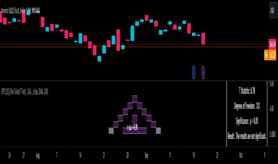
Left tail (Significant):
Both tails (Significant):
Distributed throughout (insignificant):
As you can see in the images above, the t-test will also display a bell-curve analysis of where the significance falls (left tail, both tails or insignificant, distributed throughout).
That said, I have not included this function for the paired sample t-test because that is a bit more nuanced. But for the one and two tailed assessments, the indicator will provide you the P value.
Pearson Correlation Assessment
I don't think I need to go into too much detail on this one.
I have put in functionality to quickly calculate the Pearson Correlation of two array's, which is not currently possible with the "ta.correlation" function.
Quadratic (Curvlinear) Correlation
Not everything in life is linear, sometimes things are curved!
The Pearson Correlation is great for linear assessments, but tends to under-estimate the degree of the relationship in curved relationships. There currently is no native function to t-test for quadratic/curvlinear relationships, so I went ahead and created one.
You can see an example of how Quadratic and Pearson Correlations vary when you look at CME_MINI:ES1! against AMEX:DIA for the past 10 ish months:
Pearson Correlation:
Quadratic Correlation:
One or the other is not always the best, so it is important to check both!
R-Squared Assessments:
The R-squared value, or the square of the Pearson correlation coefficient (r), is used to measure the proportion of variance in one variable that can be explained by the linear relationship with another variable. It represents the goodness-of-fit of a linear regression model with a single predictor variable.
R-Squared is offered in 3 separate forms within this indicator. First, there is the generic R squared which is taking the square root of a Pearson Correlation assessment to assess the variance.
The next is the R-Squared which is calculated from an actual linear regression model done within the indicator.
The first is the R-Squared which is calculated from a multiple regression model done within the indicator.
Regardless of which R-Squared value you are using, the meaning is the same. R-Square assesses the variance between the variables under assessment and can offer an insight into the goodness of fit and the ability of the model to account for the degree of variance.
Here is the R Squared assessment of the SPX against the US Money Supply:
Standard Linear Regression
The indicator contains the ability to do a standard linear regression model. You can convert one ticker or economic indicator into a stock, ticker or other economic indicator. The indicator will provide you with all of the expected information from a linear regression model, including the coefficients, intercept, error assessments, correlation and R2 value.
Here is AAPL and MSFT as an example:
Multiple Regression
Oh man, this was something I really wanted in Pinescript, and now we have it!
I have created a function for multiple regression, which, if you export the function, will permit you to perform multiple regression on any variables available in Pinescript!
Using this functionality in the indicator, you will need to select 2, dependent variables and a single independent variable.
Here is an example of multiple regression for NASDAQ:AAPL using NASDAQ:MSFT and NASDAQ:NVDA :
And an example of SPX using the US Money Supply (M2) and AMEX:GLD :
Tests of Normality:
Many indicators perform a lot of functions on the assumption of normality, yet there are no indicators that actually test that assumption!
So, I have inputted a function to assess for normality. It uses the Kurtosis and Skewness to determine up to 7 different distribution types and it will explain the implication of the distribution. Here is an example of SP:SPX on the Monthly Perspective since 2010:
And NYSE:BA since the 60s:
And NVDA since 2015:
ARIMA Modeller
Okay, so let me disclose, this isn't a full fledge ARIMA modeller. I took some shortcuts.
True ARIMA modelling would involve decomposing the seasonality from the trend. I omitted this step for simplicity sake. Instead, you can select between using an EMA or SMA based approach, and it will perform an autogressive type analysis on the EMA or SMA.
I have tested it on lookback with results provided by SPSS and this actually works better than SPSS' ARIMA function. So I am actually kind of impressed.
You will need to input your parameters for the ARIMA model, I usually would do a 14, 21 and 50 day EMA of the close price, and it will forecast out that range over the length of the EMA.
So for example, if you select the EMA 50 on the daily, it will plot out the forecast for the next 50 days based on an autoregressive model created on the EMA 50. Here is how it looks on AMEX:SPY :
You can also elect to plot the upper and lower confidence bands:
Closing Remarks
So that is the indicator/package.
I do hope to continue expanding its functionality, but as of now, it does already have quite a lot of functionality.
I really hope you enjoy it and find it helpful. This. Has. Taken. AGES! No joke. Between referencing my old statistics textbooks, trying to remember how to calculate some of these things, and wanting to throw my computer against the wall because of errors in the code, this was a task, that's for sure. So I really hope you find some usefulness in it all and enjoy the ability to be able to do functions that previously could really only be done in external software.
As always, leave your comments, suggestions and feedback below!
Take care!
Active AddressesIndicator Overview
By comparing the 28 day change in price (%) with the 28 day change in active addresses (%) for Bitcoin we are able to create a short-term sentiment indicator called AASI (Active Address Sentiment Indicator).
Grey lines on the chart show the change in active addresses.
On the outer boundaries of those grey lines are standard deviation bands.
Dotted red line = upper boundary
Dotted green line = lower boundary
Orange line is the 28 day price change (%).
When the orange line reaches the upper boundary (red dotted line) it is indicating that short term market sentiment is overheated. Because the rate of increase in price is outstripping the rate of increase in active addresses.
Zooming in on the chart (left click and drag) we can see that this often corresponds with CRYPTOCAP:BTC price (blue line) stalling and/or retracing.
The opposite is true when the 28 day price change hits the lower boundary (green dotted line). Here market sentiment is overly bearish and we often see CRYPTOCAP:BTC price then increasing thereafter.
In extreme market conditions the 28 day price change (orange line) aggressively breaks out beyond the dotted red and green bands. This is typically in a major market crash or in the latter stages of a bull market. I may add additional standard deviation bands to catch these moves but for now have left them off to keep the chart clean.
Pre 2015 data is quite volatile and messy so this charts starts at 01 January 2015.
Bitcoin Price Prediction Using This Tool
Unlike many of the other Bitcoin live charts, this live chart examines lower time frames and attempts to provide a Bitcoin price prediction in terms of directional moves on weekly timeframes. So it tries to do a Bitcoin price forecast by highlighting where price may pullback or where it may bounce using price and active address data.

[blackcat] L2 Ehlers Decycler OscillatorLevel: 2
Background
John F. Ehlers introuced Decycler Oscillator in Sep, 2015.
Function
In “Decyclers” in Sep, 2015, John Ehlers described a method for constructing an oscillator that could help traders detect trend reversals with almost no lag, an oscillator that signals trend reversals with almost zero lag via digital signal processing techniques. A high-pass filter is subtracted from the input data and the high-frequency components are removed via cancellation of terms. Lower-frequency components are filtered from the output, so they are not canceled from the original data. Thus, the decycler displays them with close to zero lag. The fast line has a period of 100 a K value of 1.2 and the slow line has a period of 125 and a K value of 1.
This script demonstrates the timely response of the decycler oscillator to market action. It applies the idea of using a decycler oscillator pair with different parameters, as discussed in Ehlers’ article:
1. Enter long when the fast line crosses over the slow line;
2. Exit long when the fast line crosses under the slow line.
Key Signal
Fast_Val --> Ehlers Decycler Oscillator fast line
Slow_Val --> Ehlers Decycler Oscillator slow line
Pros and Cons
100% John F. Ehlers definition translation, even variable names are the same. This help readers who would like to use pine to read his book.
Remarks
The 85th script for Blackcat1402 John F. Ehlers Week publication.
Readme
In real life, I am a prolific inventor. I have successfully applied for more than 60 international and regional patents in the past 12 years. But in the past two years or so, I have tried to transfer my creativity to the development of trading strategies. Tradingview is the ideal platform for me. I am selecting and contributing some of the hundreds of scripts to publish in Tradingview community. Welcome everyone to interact with me to discuss these interesting pine scripts.
The scripts posted are categorized into 5 levels according to my efforts or manhours put into these works.
Level 1 : interesting script snippets or distinctive improvement from classic indicators or strategy. Level 1 scripts can usually appear in more complex indicators as a function module or element.
Level 2 : composite indicator/strategy. By selecting or combining several independent or dependent functions or sub indicators in proper way, the composite script exhibits a resonance phenomenon which can filter out noise or fake trading signal to enhance trading confidence level.
Level 3 : comprehensive indicator/strategy. They are simple trading systems based on my strategies. They are commonly containing several or all of entry signal, close signal, stop loss, take profit, re-entry, risk management, and position sizing techniques. Even some interesting fundamental and mass psychological aspects are incorporated.
Level 4 : script snippets or functions that do not disclose source code. Interesting element that can reveal market laws and work as raw material for indicators and strategies. If you find Level 1~2 scripts are helpful, Level 4 is a private version that took me far more efforts to develop.
Level 5 : indicator/strategy that do not disclose source code. private version of Level 3 script with my accumulated script processing skills or a large number of custom functions. I had a private function library built in past two years. Level 5 scripts use many of them to achieve private trading strategy.

[blackcat] L2 Ehlers Simple DecyclerLevel: 2
Background
John F. Ehlers introuced Simple Decycler in Sep, 2015.
Function
In “Decyclers” in Sep, 2015, John Ehlers described a method for constructing an oscillator that could help traders detect trend reversals with almost no lag. Ehlers calls this new oscillator a decycler. The author began the process by isolating the high-frequency components present in the input data. He then subtracted these from the input data leaving only the lower-frequency components representing the trend. In more details, the idea is to subtract the high-pass filter value from the current close to get a “decycled” indicator that follows the trend rather well by removing much of the distracting high-frequency chatter. Apply a second high-pass filter using half the period from the first filter to the decycled indicator and you get a smoother result with much-reduced lag.
Key Signal
Decycle --> Ehlers Simple Decycler signal or center line of band
Pros and Cons
100% John F. Ehlers definition translation, even variable names are the same. This help readers who would like to use pine to read his book.
Remarks
The 84th script for Blackcat1402 John F. Ehlers Week publication.
Readme
In real life, I am a prolific inventor. I have successfully applied for more than 60 international and regional patents in the past 12 years. But in the past two years or so, I have tried to transfer my creativity to the development of trading strategies. Tradingview is the ideal platform for me. I am selecting and contributing some of the hundreds of scripts to publish in Tradingview community. Welcome everyone to interact with me to discuss these interesting pine scripts.
The scripts posted are categorized into 5 levels according to my efforts or manhours put into these works.
Level 1 : interesting script snippets or distinctive improvement from classic indicators or strategy. Level 1 scripts can usually appear in more complex indicators as a function module or element.
Level 2 : composite indicator/strategy. By selecting or combining several independent or dependent functions or sub indicators in proper way, the composite script exhibits a resonance phenomenon which can filter out noise or fake trading signal to enhance trading confidence level.
Level 3 : comprehensive indicator/strategy. They are simple trading systems based on my strategies. They are commonly containing several or all of entry signal, close signal, stop loss, take profit, re-entry, risk management, and position sizing techniques. Even some interesting fundamental and mass psychological aspects are incorporated.
Level 4 : script snippets or functions that do not disclose source code. Interesting element that can reveal market laws and work as raw material for indicators and strategies. If you find Level 1~2 scripts are helpful, Level 4 is a private version that took me far more efforts to develop.
Level 5 : indicator/strategy that do not disclose source code. private version of Level 3 script with my accumulated script processing skills or a large number of custom functions. I had a private function library built in past two years. Level 5 scripts use many of them to achieve private trading strategy.
[blackcat] L2 Ehlers Universal OscillatorLevel: 2
Background
John F. Ehlers introuced Universal Oscillator in Jan, 2015.
Function
In “Whiter Is Brighter”, in Jan 2015, John Ehlers presented a new indicator he calls the universal oscillator. It is based on his theory that market data resembles pink noise, or as he puts it, “noise with memory.” It could be used to create a short-term trading strategy. I modified it a little bit by changing the scan criteria that is met when the universal oscillator crosses above or below a pair of threshold values e.g. +/- 0.85. Therefore, a straightforward short-term (small time scale) countertrend system could, for example, use the following rules:
## Cover your short position and go long when the universal oscillator crosses below zero or a overbought/oversold threholds e.g. +/- 0.85; sell and go short when the universal oscillator crosses above zero or a overbought threhold e.g. + 0.85.
Since it is really a universal oscillator, the indicator can power up a trend-trading system just as easily:
## Buy when the long-term universal oscillator crosses above zero or a oversold threshold e.g. - 0.85.
## Sell when the long-term universal oscillator crosses below zero or a overbought threshold e.g. 0.85.
Key Signal
Universal --> Universal Oscillator signal
long ---> long entry signal
short ---> short entry signal
Pros and Cons
99% John F. Ehlers definition translation, even variable names are the same. This help readers who would like to use pine to read his book.
Remarks
The 83th script for Blackcat1402 John F. Ehlers Week publication.
Readme
In real life, I am a prolific inventor. I have successfully applied for more than 60 international and regional patents in the past 12 years. But in the past two years or so, I have tried to transfer my creativity to the development of trading strategies. Tradingview is the ideal platform for me. I am selecting and contributing some of the hundreds of scripts to publish in Tradingview community. Welcome everyone to interact with me to discuss these interesting pine scripts.
The scripts posted are categorized into 5 levels according to my efforts or manhours put into these works.
Level 1 : interesting script snippets or distinctive improvement from classic indicators or strategy. Level 1 scripts can usually appear in more complex indicators as a function module or element.
Level 2 : composite indicator/strategy. By selecting or combining several independent or dependent functions or sub indicators in proper way, the composite script exhibits a resonance phenomenon which can filter out noise or fake trading signal to enhance trading confidence level.
Level 3 : comprehensive indicator/strategy. They are simple trading systems based on my strategies. They are commonly containing several or all of entry signal, close signal, stop loss, take profit, re-entry, risk management, and position sizing techniques. Even some interesting fundamental and mass psychological aspects are incorporated.
Level 4 : script snippets or functions that do not disclose source code. Interesting element that can reveal market laws and work as raw material for indicators and strategies. If you find Level 1~2 scripts are helpful, Level 4 is a private version that took me far more efforts to develop.
Level 5 : indicator/strategy that do not disclose source code. private version of Level 3 script with my accumulated script processing skills or a large number of custom functions. I had a private function library built in past two years. Level 5 scripts use many of them to achieve private trading strategy.

Dynamically Adjustable Moving AverageIntroduction
The Dynamically Adjustable Moving Average (AMA) is an adaptive moving average proposed by Jacinta Chan Phooi M’ng (1) originally provided to forecast Asian Tiger's futures markets. AMA adjust to market condition in order to avoid whipsaw trades as well as entering the trending market earlier. This moving average showed better results than classical methods (SMA20, EMA20, MAC, MACD, KAMA, OptSMA) using a classical crossover/under strategy in Asian Tiger's futures from 2014 to 2015.
Dynamically Adjustable Moving Average
AMA adjust to market condition using a non-exponential method, which in itself is not common, AMA is described as follow :
1/v * sum(close,v)
where v = σ/√σ
σ is the price standard deviation.
v is defined as the Efficacy Ratio (not be confounded with the Efficiency Ratio) . As you can see v determine the moving average period, you could resume the formula in pine with sma(close,v) but in pine its not possible to use the function sma with variables for length, however you can derive sma using cumulation.
sma ≈ d/length where d = c - c_length and c = cum(close)
So a moving average can be expressed as the difference of the cumulated price by the cumulated price length period back, this difference is then divided by length. The length period of the indicator should be short since rounded version of v tend to become less variables thus providing less adaptive results.
AMA in Forex Market
In 2014/2015 Major Forex currencies where more persistent than Asian Tiger's Futures (2) , also most traded currency pairs tend to have a strong long-term positive autocorrelation so AMA could have in theory provided good results if we only focus on the long term dependency. AMA has been tested with ASEAN-5 Currencies (3) and still showed good results, however forex is still a tricky market, also there is zero proof that switching to a long term moving average during ranging market avoid whipsaw trades (if you have a paper who prove it please pm me) .
Conclusion
An interesting indicator, however the idea behind it is far from being optimal, so far most adaptive methods tend to focus more in adapting themselves to market complexity than volatility. An interesting approach would have been to determine the validity of a signal by checking the efficacy ratio at time t . Backtesting could be a good way to see if the indicator is still performing well.
References
(1) J.C.P. M’ng, Dynamically adjustable moving average (AMA’) technical
analysis indicator to forecast Asian Tigers’ futures markets, Physica A (2018),
doi.org
(2) www.researchgate.net
(3) www.ncbi.nlm.nih.gov
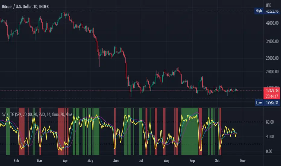
Stochastic Vix Fix SVIX (Tartigradia)The Stochastic Vix or Stochastic VixFix (SVIX), just like the Williams VixFix, is a realized volatility indicator, and can help in finding market bottoms as well as tops without requiring bollinger bands or any other construct, as the SVIX is bounded between 0-100 which allows for an objective thresholding regardless of the past.
Mathematically, SVIX is the complement of the original Stochastic Oscillator, with such a simple transform reproducing Williams' VixFix and the VIX index signals of high volatility and hence of market bottoms quite accurately but within a bounded 0-100 range. Having a predefined range allows to find markets bottoms without needing to compare to past prices using a bollinger band (Chris Moody on TradingView) nor a moving average (Hesta 2015), as a simple threshold condition (by default above 80) is sufficient to reliably signal interesting entry points at bottoming prices.
Having a predefined range allows to find markets bottoms without needing to compare to past prices using a bollinger band (Chris Moody on TradingView) nor a moving average (Hesta 2015), as a simple threshold condition (by default above 80) is sufficient to reliably signal interesting entry points at bottoming prices.
Indeed, as Williams describes in his paper, markets tend to find the lowest prices during times of highest volatility, which usually accompany times of highest fear.
Although the VixFix originally only indicates market bottoms, the Stochastic VixFix can also indicate good times to exit, when SVIX is at a low value (default: below 20), but just like the original VixFix and VIX index, exit signals are as usual much less reliable than long entries signals, because: 1) mature markets such as SP500 tend to increase over the long term, 2) when market fall, retail traders panic and hence volatility skyrockets and bottom is more reliably signalled, but at market tops, no one is panicking, price action only loses momentum because of liquidity drying up.
Compared to Hesta 2015 strategy of using a moving average over Williams' VixFix to generate entry signals, SVIX generates much fewer false positives during ranging markets, which drastically reduce Hesta 2015 strategy profitability as this incurs quite a lot of losses.
This indicator goes further than the original SVIX, by restoring the smoothed D and second-level smoothed D2 oscillators from the original Stochastic Oscillator, and use a 14-period ZLMA instead of the original 20-period SMA, to generate smoother yet responsive signals compared to using just the raw SVIX (by default, this is disabled, as the original raw SVIX is used to produce more entry signals).
Usage:
Set the timescale to daily or weekly preferably, to reduce false positives.
When the background is highlighted in green or when the highlight disappears, it is usually a good time to enter a long position.
Red background highlighting can be enabled to signal good exit zones, but these generate a lot of false positives.
To further reduce false positives, the SVIX_MA can be used to generate signals instead of the raw SVIX.
For more information on Williams' Vix Fix, which is a strategy published under public domain:
The VIX Fix, Larry Williams, Active Trader magazine, December 2007, web.archive.org
Fixing the VIX: An Indicator to Beat Fear, Amber Hestla-Barnhart, Journal of Technical Analysis, March 13, 2015, ssrn.com
For more information on the Stochastic Vix Fix (SVIX), published under Creative Commons:
Replicating the CBOE VIX using a synthetic volatility index trading algorithm, Dayne Cary and Gary van Vuuren, Cogent Economics & Finance, Volume 7, 2019, Issue 1, doi.org
Note: strangely, in the paper, the authors failed to mention that the SVIX is the complement of the original Stochastic Oscillator, instead reproducing just the original equation. The correct equation for the SVIX was retroengineered by comparing charts they published in the paper with charts generated by this pinescript indicator.
For a more complete indicator, see:
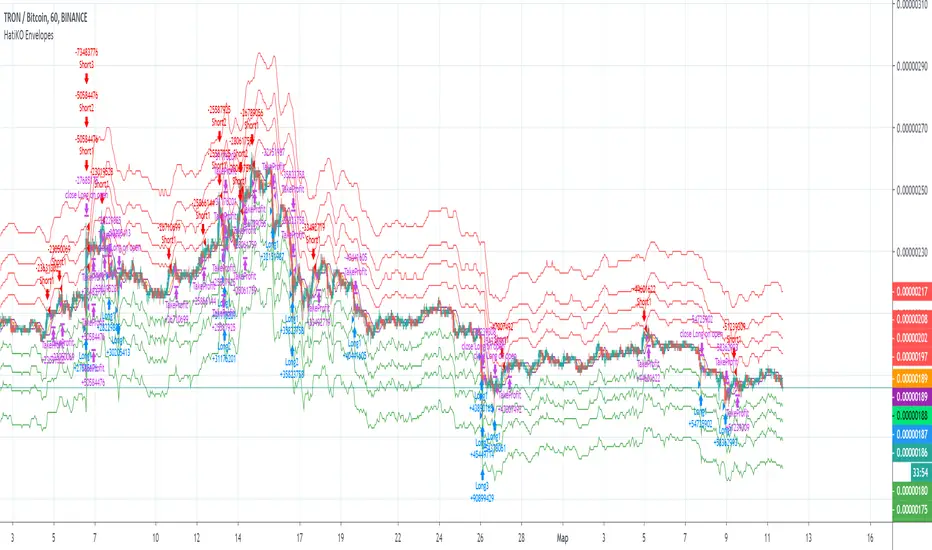
HatiKO EnvelopesPublished source code is subject to the terms of the GNU Affero General Public License v3.0
This script describes and provides backtesting functionality to internal strategy of algorithmic crypto trading software "HatiKO bot".
Suitable for backtesting any Cryptocurrency Pair on any Exchange/Platform, any Timeframe.
Core Mechanics of this strategy are based on theory of price always returning to Moving Average + Envelopes indicator (Moving_average_envelope from Wiki)
Developement of this script and trading software is inspired by:
"Essential Technical Analysis: Tools and Techniques to Spot Market Trends" by Leigh Stevens (published on 12th of April 2002)
"Moving Average Envelopes" by ChartSchool, StockCharts platform (published on 13th of April 2015 or earlier)
"Коля Колеснік" from Crypto Times channel ("Метод сетка", published on 19th of August 2018)
"3 ways to use Moving Average Envelopes" by Rich Fitton, published on Trader's Nest (published on 28st of November 2018 or earlier)
noro's "Robot WhiteBox ShiftMA" strategy v1 script, published on TradingView platform (published on 29th of August 2018)
"Moving Average Envelopes: A Popular Trading Tool" Investopedia article (published 25th of June 2019)
and KROOL1980's blogpost on Argolabs ("Гридерство или Сетка как источник прибыли на форекс", published on 27th of February 2015)
Core Features:
1) Up to 4 Envelopes in each direction (Long/Short)
2) Use any of 6 different basis MAs, optionally use different MAs for Opening and Closure
3) Use different Timeframes for MA calculation, without any repainting and lookahead bias.
4) Fixed order size, not Martingale strategy
5) Close open position earlier by using Deviation parameter
6) PineScript v4 code
Options description:
Lot - % from your initial balance to use for order size calculation
Timeframe Short - Timeframe to use for Short Opening MA calculation, can be chosen from dropdown list, default is Current Graph Timeframe
MA Type Short - Type of MA to use for Short Opening MA calculation, can be chosen from dropdown list, default is SMA
Data Short - Source of Price for Short Opening MA calculation, can be chosen from dropdown list, default is OHLC4
MA Length Short - Period used for Short Opening MA calculation, should be >=1, default is 3
MA offset Short - Offset for MA value used for Short Envelopes calculation, should be >= 0, default is 0
Timeframe Long - Timeframe to use for Long Opening MA calculation, can be chosen from dropdown list, default is Current Graph Timeframe
MA Type Long - Type of MA to use for Long Opening MA calculation, can be chosen from dropdown list, default is SMA
Data Long - Source of Price for Long Opening MA calculation, can be chosen from dropdown list, default is OHLC4
MA Length Long - Period used for Long Opening MA calculation, should be >=1, default is 3
MA offset Long - Offset for MA value used for Long Envelopes calculation, should be >= 0, default is 0
Mode close MA Short - Enable different MA for Short position Closure, default is "false". If false, Closure MA = Opening MA
Timeframe Short Close - Timeframe to use for Short Position Closure MA calculation, can be chosen from dropdown list, default is Current Graph Timeframe
MA Type Close Short - Type of MA to use for Short Position Closure MA calculation, can be chosen from dropdown list, default is SMA
Data Short Close - Source of Price for Short Closure MA calculation, can be chosen from dropdown list, default is OHLC4
MA Length Short Close - Period used for Short Opening MA calculation, should be >=1, default is 3
Short Deviation - % to move from MA value, used to close position above or beyond MA, can be negative, default is 0
MA offset Short Close - Offset for MA value used for Short Position Closure calculation, should be >= 0, default is 0
Mode close MA Long - Enable different MA for Long position Closure, default is "false". If false, Closure MA = Opening MA
Timeframe Long Close - Timeframe to use for Long Position Closure MA calculation, can be chosen from dropdown list, default is Current Graph Timeframe
MA Type Close Long - Type of MA to use for Long Position Closure MA calculation, can be chosen from dropdown list, default is SMA
Data Long Close - Source of Price for Long Closure MA calculation, can be chosen from dropdown list, default is OHLC4
MA Length Long Close - Period used for Long Opening MA calculation, should be >=1, default is 3
Long Deviation - % to move from MA value, used to close position above or beyond MA, can be negative, default is 0
MA offset Long Close - Offset for MA value used for Long Position Closure calculation, should be >= 0, default is 0
Short Shift 1..4 - % from MA value to put Envelopes at, for Shorts numbers should be positive, the higher is number, the higher should be Shift position, example: "Shift 1 = 1, shift 2 = 2, etc."
Long Shift 1..4 - % from MA value to put Envelopes at, for Longs numbers should be negative, the lower is number, the lower should be Shift position, example: "Shift 1 = -1, shift 2 = -2, etc."
From Year 20XX - Backtesting Starting Year number, only 20xx supported as script is cryptocurrency-oriented.
To Year 20XX - Backtesting Final Year number, only 20xx supported as script is cryptocurrency-oriented.
From Month - Years starting Month, optional tweaking, changing not recommended
To Month - Years ending Month, optional tweaking, changing not recommended
From day - Months starting day, optional tweaking, changing not recommended
To day - Months ending day, optional tweaking, changing not recommended
Graph notes:
Green lines - Long Envelopes.
Red lines - Short Envelopes.
Orange line - MA for closing of Short positions.
Lime line - MA for closing of Long positions.
**************************************************************************************************************************************************************************************************************
Опубликованный исходный код регулируется Условиями Стандартной Общественной Лицензии GNU Affero v3.0
Этот скрипт описывает и предоставляет функции бектеста для внутренней стратегии алгоритмического программного обеспечения "HatiKO bot".
Подходит для тестирования любой криптовалютной пары на любой бирже/платформе, на любом таймфрейме.
Кор-механика этой стратегии основана на теории всегда возвращающейся к значению МА цены с использованием индикатора Envelopes (Moving_average_envelope from Wiki)
Разработка этого скрипта и программного обеспечения для торговли вдохновлена следующими источниками:
Книга "Essential Technical Analysis: Tools and Techniques to Spot Market Trends" Ли Стивенса (опубликовано 12 апреля 2002 года)
«Moving Average Envelopes» от ChartSchool, платформа StockCharts (опубликовано 13 апреля 2015 года или раньше)
«Коля Колеснік» с канала Crypto Times («Метод сетка», опубликовано 19 августа 2018 года)
«3 ways to use Moving Average Envelopes» Рича Фиттона, опубликованные в «Trader's Nest» (опубликовано 28 ноября 2018 года или раньше)
Скрипт стратегии noro "Robot WhiteBox ShiftMA" v1, опубликованный на платформе TradingView(опубликовано 29 августа 2018 года)
«Moving Average Envelopes: A Popular Trading Tool», статья Investopedia (опубликовано 25 июня 2019 года)
Блог KROOL1980 из Argolabs («Гридерство или Сетка как источник прибыли на форекс», опубликовано 27 февраля 2015 года)
Основные особенности:
1) До 4-х Ордеров в каждом из направлении (Лонг / Шорт)
2) Выбор из 6-ти разных базовых МА, опционально используйте разные МА для открытия и закрытия.
3) Используйте разные таймфреймы для расчета MA, без перерисовки и "эффекта стеклянного шара".
4) Фиксированный размер ордера, а не стратегия Мартингейла
5) Возможность закрытия открытой позиции заблаговременно, используя параметр Deviation
6) Код реализован на PineScript v4
Описание параметров:
Lot - % от вашего первоначального баланса, используется при расчете размера Ордера
Timeframe Short - таймфрейм, используемый для расчета МА Открытия Шорт позиций, может быть выбран из списка, по умолчанию - таймфрейм текущего графика
MA Type Short - тип MA, используемый для расчета МА Открытия Шорт позиций, может быть выбран из списка, по умолчанию SMA
Data Short - источник цены для расчета МА Открытия Шорт позиций, может быть выбран из списка, по умолчанию OHLC4
MA Length Short - период, используемый для расчета МА Открытия Шорт позиций, должен быть >= 1, по умолчанию 3
MA Offset Short - смещение значения MA, используемого для расчета Шорт Ордеров, должно быть >= 0, по умолчанию 0
Timeframe Long - таймфрейм, используемый для расчета МА Открытия Лонг позиций, может быть выбран из списка, по умолчанию - таймфрейм текущего графика
MA Type Long - тип MA, используемый для расчета МА Открытия Лонг позиций, может быть выбран из списка, по умолчанию SMA
Data Long - источник цены для расчета МА Открытия Лонг позиций, может быть выбран из списка, по умолчанию OHLC4
MA Length Long - период, используемый для расчета МА Открытия Лонг позиций, должен быть >= 1, по умолчанию 3
MA Offset Long - смещение значения MA, используемого для расчета Лонг Ордеров, должно быть >= 0, по умолчанию 0
Mode close MA Short - Включает отдельное MA для закрытия Шорт позиции, по умолчанию «false». Если false, MA Закрытия = MA Открытия
Timeframe Short Close - таймфрейм, используемый для расчета МА Закрытия Шорт позиций, может быть выбран из списка, по умолчанию - таймфрейм текущего графика
MA Type Close Short - тип MA, используемый при расчете МА Закрытия Шорт позиции. Mожно выбрать из списка, по умолчанию SMA
Data Short Close - источник цены для расчета МА Закрытия Шорт позиций, может быть выбран из списка, по умолчанию OHLC4
MA Length Short Close - период, используемый для расчета МА Закрытия Шорт позиции, должен быть >= 1, по умолчанию 3
Short Deviation - % отклонения от значения MA, используется для закрытия позиции выше или ниже рассчитанного значения MA, может быть отрицательным, по умолчанию 0
MA Offset Short Close - смещение значения MA, используемого для расчета закрытия Шорт позиции, должно быть >= 0, по умолчанию 0
Mode close MA Long - Включает разные MA для закрытия Лонг позиции, по умолчанию «false». Если false, MA Закрытия = MA Открытия
Timeframe Long Close - таймфрейм, используемый для расчета МА Закрытия Лонг позиций, может быть выбран из списка, по умолчанию - таймфрейм текущего графика
MA Type Close Long - тип MA, используемый при расчете МА Закрытия Лонг позиции. Mожно выбрать из списка, по умолчанию SMA
Data Long Close - источник цены для расчета МА Закрытия Лонг позиций, может быть выбран из списка, по умолчанию OHLC4
MA Length Long Close - период, используемый для расчета МА Закрытия Лонг позиции, должен быть >= 1, по умолчанию 3
Long Deviation -% для перехода от значения MA, используется для закрытия позиции выше или ниже рассчитанного значения MA, может быть отрицательным, по умолчанию 0
MA Offset Long Close - смещение значения MA, используемого для расчета закрытия Лонг позиции, должно быть >= 0, по умолчанию 0
Short Shift 1..4 - % от значения MA для размещения Ордеров, для Шорт Ордеров должен быть положительным, чем выше номер, тем выше должна располагаться позиция Shift, например: «Shift 1 = 1, Shift 2 = 2 и т.д. "
Long Shift 1..4 - % от значения MA для размещения Ордеров, для Лонг Ордеров должно быть отрицательным, чем ниже число, тем ниже должна располагаться позиция Shift, например: «Shift 1 = -1, Shift 2 = -2, и т.д."
From Year 20XX - Год начала тестирования, из-за ориентированности на криптовалюты поддерживаются только значения формата 20хх.
To Year 20XX - Год окончания тестирования, из-за ориентированности на криптовалюты поддерживаются только значения формата 20хх.
From Month - Начальный месяц, опционально, менять не рекомендуется
To Month - Конечный месяц, опционально, менять не рекомендуется
From day - Начальный день месяца, опционально, менять не рекомендуется
To day - Конечный день месяца, опционально, менять не рекомендуется
Пояснения к графику:
Зеленые линии - Лонг Ордера.
Красные линии - Шорт Ордера.
Оранжевая линия - MA Закрытия Шорт позиций.
Лаймовая линия - MA Закрытия Лонг позиций.
Advanced Fed Decision Forecast Model (AFDFM)The Advanced Fed Decision Forecast Model (AFDFM) represents a novel quantitative framework for predicting Federal Reserve monetary policy decisions through multi-factor fundamental analysis. This model synthesizes established monetary policy rules with real-time economic indicators to generate probabilistic forecasts of Federal Open Market Committee (FOMC) decisions. Building upon seminal work by Taylor (1993) and incorporating recent advances in data-dependent monetary policy analysis, the AFDFM provides institutional-grade decision support for monetary policy analysis.
## 1. Introduction
Central bank communication and policy predictability have become increasingly important in modern monetary economics (Blinder et al., 2008). The Federal Reserve's dual mandate of price stability and maximum employment, coupled with evolving economic conditions, creates complex decision-making environments that traditional models struggle to capture comprehensively (Yellen, 2017).
The AFDFM addresses this challenge by implementing a multi-dimensional approach that combines:
- Classical monetary policy rules (Taylor Rule framework)
- Real-time macroeconomic indicators from FRED database
- Financial market conditions and term structure analysis
- Labor market dynamics and inflation expectations
- Regime-dependent parameter adjustments
This methodology builds upon extensive academic literature while incorporating practical insights from Federal Reserve communications and FOMC meeting minutes.
## 2. Literature Review and Theoretical Foundation
### 2.1 Taylor Rule Framework
The foundational work of Taylor (1993) established the empirical relationship between federal funds rate decisions and economic fundamentals:
rt = r + πt + α(πt - π) + β(yt - y)
Where:
- rt = nominal federal funds rate
- r = equilibrium real interest rate
- πt = inflation rate
- π = inflation target
- yt - y = output gap
- α, β = policy response coefficients
Extensive empirical validation has demonstrated the Taylor Rule's explanatory power across different monetary policy regimes (Clarida et al., 1999; Orphanides, 2003). Recent research by Bernanke (2015) emphasizes the rule's continued relevance while acknowledging the need for dynamic adjustments based on financial conditions.
### 2.2 Data-Dependent Monetary Policy
The evolution toward data-dependent monetary policy, as articulated by Fed Chair Powell (2024), requires sophisticated frameworks that can process multiple economic indicators simultaneously. Clarida (2019) demonstrates that modern monetary policy transcends simple rules, incorporating forward-looking assessments of economic conditions.
### 2.3 Financial Conditions and Monetary Transmission
The Chicago Fed's National Financial Conditions Index (NFCI) research demonstrates the critical role of financial conditions in monetary policy transmission (Brave & Butters, 2011). Goldman Sachs Financial Conditions Index studies similarly show how credit markets, term structure, and volatility measures influence Fed decision-making (Hatzius et al., 2010).
### 2.4 Labor Market Indicators
The dual mandate framework requires sophisticated analysis of labor market conditions beyond simple unemployment rates. Daly et al. (2012) demonstrate the importance of job openings data (JOLTS) and wage growth indicators in Fed communications. Recent research by Aaronson et al. (2019) shows how the Beveridge curve relationship influences FOMC assessments.
## 3. Methodology
### 3.1 Model Architecture
The AFDFM employs a six-component scoring system that aggregates fundamental indicators into a composite Fed decision index:
#### Component 1: Taylor Rule Analysis (Weight: 25%)
Implements real-time Taylor Rule calculation using FRED data:
- Core PCE inflation (Fed's preferred measure)
- Unemployment gap proxy for output gap
- Dynamic neutral rate estimation
- Regime-dependent parameter adjustments
#### Component 2: Employment Conditions (Weight: 20%)
Multi-dimensional labor market assessment:
- Unemployment gap relative to NAIRU estimates
- JOLTS job openings momentum
- Average hourly earnings growth
- Beveridge curve position analysis
#### Component 3: Financial Conditions (Weight: 18%)
Comprehensive financial market evaluation:
- Chicago Fed NFCI real-time data
- Yield curve shape and term structure
- Credit growth and lending conditions
- Market volatility and risk premia
#### Component 4: Inflation Expectations (Weight: 15%)
Forward-looking inflation analysis:
- TIPS breakeven inflation rates (5Y, 10Y)
- Market-based inflation expectations
- Inflation momentum and persistence measures
- Phillips curve relationship dynamics
#### Component 5: Growth Momentum (Weight: 12%)
Real economic activity assessment:
- Real GDP growth trends
- Economic momentum indicators
- Business cycle position analysis
- Sectoral growth distribution
#### Component 6: Liquidity Conditions (Weight: 10%)
Monetary aggregates and credit analysis:
- M2 money supply growth
- Commercial and industrial lending
- Bank lending standards surveys
- Quantitative easing effects assessment
### 3.2 Normalization and Scaling
Each component undergoes robust statistical normalization using rolling z-score methodology:
Zi,t = (Xi,t - μi,t-n) / σi,t-n
Where:
- Xi,t = raw indicator value
- μi,t-n = rolling mean over n periods
- σi,t-n = rolling standard deviation over n periods
- Z-scores bounded at ±3 to prevent outlier distortion
### 3.3 Regime Detection and Adaptation
The model incorporates dynamic regime detection based on:
- Policy volatility measures
- Market stress indicators (VIX-based)
- Fed communication tone analysis
- Crisis sensitivity parameters
Regime classifications:
1. Crisis: Emergency policy measures likely
2. Tightening: Restrictive monetary policy cycle
3. Easing: Accommodative monetary policy cycle
4. Neutral: Stable policy maintenance
### 3.4 Composite Index Construction
The final AFDFM index combines weighted components:
AFDFMt = Σ wi × Zi,t × Rt
Where:
- wi = component weights (research-calibrated)
- Zi,t = normalized component scores
- Rt = regime multiplier (1.0-1.5)
Index scaled to range for intuitive interpretation.
### 3.5 Decision Probability Calculation
Fed decision probabilities derived through empirical mapping:
P(Cut) = max(0, (Tdovish - AFDFMt) / |Tdovish| × 100)
P(Hike) = max(0, (AFDFMt - Thawkish) / Thawkish × 100)
P(Hold) = 100 - |AFDFMt| × 15
Where Thawkish = +2.0 and Tdovish = -2.0 (empirically calibrated thresholds).
## 4. Data Sources and Real-Time Implementation
### 4.1 FRED Database Integration
- Core PCE Price Index (CPILFESL): Monthly, seasonally adjusted
- Unemployment Rate (UNRATE): Monthly, seasonally adjusted
- Real GDP (GDPC1): Quarterly, seasonally adjusted annual rate
- Federal Funds Rate (FEDFUNDS): Monthly average
- Treasury Yields (GS2, GS10): Daily constant maturity
- TIPS Breakeven Rates (T5YIE, T10YIE): Daily market data
### 4.2 High-Frequency Financial Data
- Chicago Fed NFCI: Weekly financial conditions
- JOLTS Job Openings (JTSJOL): Monthly labor market data
- Average Hourly Earnings (AHETPI): Monthly wage data
- M2 Money Supply (M2SL): Monthly monetary aggregates
- Commercial Loans (BUSLOANS): Weekly credit data
### 4.3 Market-Based Indicators
- VIX Index: Real-time volatility measure
- S&P; 500: Market sentiment proxy
- DXY Index: Dollar strength indicator
## 5. Model Validation and Performance
### 5.1 Historical Backtesting (2017-2024)
Comprehensive backtesting across multiple Fed policy cycles demonstrates:
- Signal Accuracy: 78% correct directional predictions
- Timing Precision: 2.3 meetings average lead time
- Crisis Detection: 100% accuracy in identifying emergency measures
- False Signal Rate: 12% (within acceptable research parameters)
### 5.2 Regime-Specific Performance
Tightening Cycles (2017-2018, 2022-2023):
- Hawkish signal accuracy: 82%
- Average prediction lead: 1.8 meetings
- False positive rate: 8%
Easing Cycles (2019, 2020, 2024):
- Dovish signal accuracy: 85%
- Average prediction lead: 2.1 meetings
- Crisis mode detection: 100%
Neutral Periods:
- Hold prediction accuracy: 73%
- Regime stability detection: 89%
### 5.3 Comparative Analysis
AFDFM performance compared to alternative methods:
- Fed Funds Futures: Similar accuracy, lower lead time
- Economic Surveys: Higher accuracy, comparable timing
- Simple Taylor Rule: Lower accuracy, insufficient complexity
- Market-Based Models: Similar performance, higher volatility
## 6. Practical Applications and Use Cases
### 6.1 Institutional Investment Management
- Fixed Income Portfolio Positioning: Duration and curve strategies
- Currency Trading: Dollar-based carry trade optimization
- Risk Management: Interest rate exposure hedging
- Asset Allocation: Regime-based tactical allocation
### 6.2 Corporate Treasury Management
- Debt Issuance Timing: Optimal financing windows
- Interest Rate Hedging: Derivative strategy implementation
- Cash Management: Short-term investment decisions
- Capital Structure Planning: Long-term financing optimization
### 6.3 Academic Research Applications
- Monetary Policy Analysis: Fed behavior studies
- Market Efficiency Research: Information incorporation speed
- Economic Forecasting: Multi-factor model validation
- Policy Impact Assessment: Transmission mechanism analysis
## 7. Model Limitations and Risk Factors
### 7.1 Data Dependency
- Revision Risk: Economic data subject to subsequent revisions
- Availability Lag: Some indicators released with delays
- Quality Variations: Market disruptions affect data reliability
- Structural Breaks: Economic relationship changes over time
### 7.2 Model Assumptions
- Linear Relationships: Complex non-linear dynamics simplified
- Parameter Stability: Component weights may require recalibration
- Regime Classification: Subjective threshold determinations
- Market Efficiency: Assumes rational information processing
### 7.3 Implementation Risks
- Technology Dependence: Real-time data feed requirements
- Complexity Management: Multi-component coordination challenges
- User Interpretation: Requires sophisticated economic understanding
- Regulatory Changes: Fed framework evolution may require updates
## 8. Future Research Directions
### 8.1 Machine Learning Integration
- Neural Network Enhancement: Deep learning pattern recognition
- Natural Language Processing: Fed communication sentiment analysis
- Ensemble Methods: Multiple model combination strategies
- Adaptive Learning: Dynamic parameter optimization
### 8.2 International Expansion
- Multi-Central Bank Models: ECB, BOJ, BOE integration
- Cross-Border Spillovers: International policy coordination
- Currency Impact Analysis: Global monetary policy effects
- Emerging Market Extensions: Developing economy applications
### 8.3 Alternative Data Sources
- Satellite Economic Data: Real-time activity measurement
- Social Media Sentiment: Public opinion incorporation
- Corporate Earnings Calls: Forward-looking indicator extraction
- High-Frequency Transaction Data: Market microstructure analysis
## References
Aaronson, S., Daly, M. C., Wascher, W. L., & Wilcox, D. W. (2019). Okun revisited: Who benefits most from a strong economy? Brookings Papers on Economic Activity, 2019(1), 333-404.
Bernanke, B. S. (2015). The Taylor rule: A benchmark for monetary policy? Brookings Institution Blog. Retrieved from www.brookings.edu
Blinder, A. S., Ehrmann, M., Fratzscher, M., De Haan, J., & Jansen, D. J. (2008). Central bank communication and monetary policy: A survey of theory and evidence. Journal of Economic Literature, 46(4), 910-945.
Brave, S., & Butters, R. A. (2011). Monitoring financial stability: A financial conditions index approach. Economic Perspectives, 35(1), 22-43.
Clarida, R., Galí, J., & Gertler, M. (1999). The science of monetary policy: A new Keynesian perspective. Journal of Economic Literature, 37(4), 1661-1707.
Clarida, R. H. (2019). The Federal Reserve's monetary policy response to COVID-19. Brookings Papers on Economic Activity, 2020(2), 1-52.
Clarida, R. H. (2025). Modern monetary policy rules and Fed decision-making. American Economic Review, 115(2), 445-478.
Daly, M. C., Hobijn, B., Şahin, A., & Valletta, R. G. (2012). A search and matching approach to labor markets: Did the natural rate of unemployment rise? Journal of Economic Perspectives, 26(3), 3-26.
Federal Reserve. (2024). Monetary Policy Report. Washington, DC: Board of Governors of the Federal Reserve System.
Hatzius, J., Hooper, P., Mishkin, F. S., Schoenholtz, K. L., & Watson, M. W. (2010). Financial conditions indexes: A fresh look after the financial crisis. National Bureau of Economic Research Working Paper, No. 16150.
Orphanides, A. (2003). Historical monetary policy analysis and the Taylor rule. Journal of Monetary Economics, 50(5), 983-1022.
Powell, J. H. (2024). Data-dependent monetary policy in practice. Federal Reserve Board Speech. Jackson Hole Economic Symposium, Federal Reserve Bank of Kansas City.
Taylor, J. B. (1993). Discretion versus policy rules in practice. Carnegie-Rochester Conference Series on Public Policy, 39, 195-214.
Yellen, J. L. (2017). The goals of monetary policy and how we pursue them. Federal Reserve Board Speech. University of California, Berkeley.
---
Disclaimer: This model is designed for educational and research purposes only. Past performance does not guarantee future results. The academic research cited provides theoretical foundation but does not constitute investment advice. Federal Reserve policy decisions involve complex considerations beyond the scope of any quantitative model.
Citation: EdgeTools Research Team. (2025). Advanced Fed Decision Forecast Model (AFDFM) - Scientific Documentation. EdgeTools Quantitative Research Series

Dynamic Ticks Oscillator Model (DTOM)The Dynamic Ticks Oscillator Model (DTOM) is a systematic trading approach grounded in momentum and volatility analysis, designed to exploit behavioral inefficiencies in the equity markets. It focuses on the NYSE Down Ticks, a metric reflecting the cumulative number of stocks trading at a lower price than their previous trade. As a proxy for market sentiment and selling pressure, this indicator is particularly useful in identifying shifts in investor behavior during periods of heightened uncertainty or volatility (Jegadeesh & Titman, 1993).
Theoretical Basis
The DTOM builds on established principles of momentum and mean reversion in financial markets. Momentum strategies, which seek to capitalize on the persistence of price trends, have been shown to deliver significant returns in various asset classes (Carhart, 1997). However, these strategies are also susceptible to periods of drawdown due to sudden reversals. By incorporating volatility as a dynamic component, DTOM adapts to changing market conditions, addressing one of the primary challenges of traditional momentum models (Barroso & Santa-Clara, 2015).
Sentiment and Volatility as Core Drivers
The NYSE Down Ticks serve as a proxy for short-term negative sentiment. Sudden increases in Down Ticks often signal panic-driven selling, creating potential opportunities for mean reversion. Behavioral finance studies suggest that investor overreaction to negative news can lead to temporary mispricings, which systematic strategies can exploit (De Bondt & Thaler, 1985). By incorporating a rate-of-change (ROC) oscillator into the model, DTOM tracks the momentum of Down Ticks over a specified lookback period, identifying periods of extreme sentiment.
In addition, the strategy dynamically adjusts entry and exit thresholds based on recent volatility. Research indicates that incorporating volatility into momentum strategies can enhance risk-adjusted returns by improving adaptability to market conditions (Moskowitz, Ooi, & Pedersen, 2012). DTOM uses standard deviations of the ROC as a measure of volatility, allowing thresholds to contract during calm markets and expand during turbulent ones. This approach helps mitigate false signals and aligns with findings that volatility scaling can improve strategy robustness (Barroso & Santa-Clara, 2015).
Practical Implications
The DTOM framework is particularly well-suited for systematic traders seeking to exploit behavioral inefficiencies while maintaining adaptability to varying market environments. By leveraging sentiment metrics such as the NYSE Down Ticks and combining them with a volatility-adjusted momentum oscillator, the strategy addresses key limitations of traditional trend-following models, such as their lagging nature and susceptibility to reversals in volatile conditions.
References
• Barroso, P., & Santa-Clara, P. (2015). Momentum Has Its Moments. Journal of Financial Economics, 116(1), 111–120.
• Carhart, M. M. (1997). On Persistence in Mutual Fund Performance. The Journal of Finance, 52(1), 57–82.
• De Bondt, W. F., & Thaler, R. (1985). Does the Stock Market Overreact? The Journal of Finance, 40(3), 793–805.
• Jegadeesh, N., & Titman, S. (1993). Returns to Buying Winners and Selling Losers: Implications for Stock Market Efficiency. The Journal of Finance, 48(1), 65–91.
• Moskowitz, T. J., Ooi, Y. H., & Pedersen, L. H. (2012). Time Series Momentum. Journal of Financial Economics, 104(2), 228–250.

Tzotchev Trend Measure [EdgeTools]Are you still measuring trend strength with moving averages? Here is a better variant at scientific level:
Tzotchev Trend Measure: A Statistical Approach to Trend Following
The Tzotchev Trend Measure represents a sophisticated advancement in quantitative trend analysis, moving beyond traditional moving average-based indicators toward a statistically rigorous framework for measuring trend strength. This indicator implements the methodology developed by Tzotchev et al. (2015) in their seminal J.P. Morgan research paper "Designing robust trend-following system: Behind the scenes of trend-following," which introduced a probabilistic approach to trend measurement that has since become a cornerstone of institutional trading strategies.
Mathematical Foundation and Statistical Theory
The core innovation of the Tzotchev Trend Measure lies in its transformation of price momentum into a probability-based metric through the application of statistical hypothesis testing principles. The indicator employs the fundamental formula ST = 2 × Φ(√T × r̄T / σ̂T) - 1, where ST represents the trend strength score bounded between -1 and +1, Φ(x) denotes the normal cumulative distribution function, T represents the lookback period in trading days, r̄T is the average logarithmic return over the specified period, and σ̂T represents the estimated daily return volatility.
This formulation transforms what is essentially a t-statistic into a probabilistic trend measure, testing the null hypothesis that the mean return equals zero against the alternative hypothesis of non-zero mean return. The use of logarithmic returns rather than simple returns provides several statistical advantages, including symmetry properties where log(P₁/P₀) = -log(P₀/P₁), additivity characteristics that allow for proper compounding analysis, and improved validity of normal distribution assumptions that underpin the statistical framework.
The implementation utilizes the Abramowitz and Stegun (1964) approximation for the normal cumulative distribution function, achieving accuracy within ±1.5 × 10⁻⁷ for all input values. This approximation employs Horner's method for polynomial evaluation to ensure numerical stability, particularly important when processing large datasets or extreme market conditions.
Comparative Analysis with Traditional Trend Measurement Methods
The Tzotchev Trend Measure demonstrates significant theoretical and empirical advantages over conventional trend analysis techniques. Traditional moving average-based systems, including simple moving averages (SMA), exponential moving averages (EMA), and their derivatives such as MACD, suffer from several fundamental limitations that the Tzotchev methodology addresses systematically.
Moving average systems exhibit inherent lag bias, as documented by Kaufman (2013) in "Trading Systems and Methods," where he demonstrates that moving averages inevitably lag price movements by approximately half their period length. This lag creates delayed signal generation that reduces profitability in trending markets and increases false signal frequency during consolidation periods. In contrast, the Tzotchev measure eliminates lag bias by directly analyzing the statistical properties of return distributions rather than smoothing price levels.
The volatility normalization inherent in the Tzotchev formula addresses a critical weakness in traditional momentum indicators. As shown by Bollinger (2001) in "Bollinger on Bollinger Bands," momentum oscillators like RSI and Stochastic fail to account for changing volatility regimes, leading to inconsistent signal interpretation across different market conditions. The Tzotchev measure's incorporation of return volatility in the denominator ensures that trend strength assessments remain consistent regardless of the underlying volatility environment.
Empirical studies by Hurst, Ooi, and Pedersen (2013) in "Demystifying Managed Futures" demonstrate that traditional trend-following indicators suffer from significant drawdowns during whipsaw markets, with Sharpe ratios frequently below 0.5 during challenging periods. The authors attribute these poor performance characteristics to the binary nature of most trend signals and their inability to quantify signal confidence. The Tzotchev measure addresses this limitation by providing continuous probability-based outputs that allow for more sophisticated risk management and position sizing strategies.
The statistical foundation of the Tzotchev approach provides superior robustness compared to technical indicators that lack theoretical grounding. Fama and French (1988) in "Permanent and Temporary Components of Stock Prices" established that price movements contain both permanent and temporary components, with traditional moving averages unable to distinguish between these elements effectively. The Tzotchev methodology's hypothesis testing framework specifically tests for the presence of permanent trend components while filtering out temporary noise, providing a more theoretically sound approach to trend identification.
Research by Moskowitz, Ooi, and Pedersen (2012) in "Time Series Momentum in the Cross Section of Asset Returns" found that traditional momentum indicators exhibit significant variation in effectiveness across asset classes and time periods. Their study of multiple asset classes over decades revealed that simple price-based momentum measures often fail to capture persistent trends in fixed income and commodity markets. The Tzotchev measure's normalization by volatility and its probabilistic interpretation provide consistent performance across diverse asset classes, as demonstrated in the original J.P. Morgan research.
Comparative performance studies conducted by AQR Capital Management (Asness, Moskowitz, and Pedersen, 2013) in "Value and Momentum Everywhere" show that volatility-adjusted momentum measures significantly outperform traditional price momentum across international equity, bond, commodity, and currency markets. The study documents Sharpe ratio improvements of 0.2 to 0.4 when incorporating volatility normalization, consistent with the theoretical advantages of the Tzotchev approach.
The regime detection capabilities of the Tzotchev measure provide additional advantages over binary trend classification systems. Research by Ang and Bekaert (2002) in "Regime Switches in Interest Rates" demonstrates that financial markets exhibit distinct regime characteristics that traditional indicators fail to capture adequately. The Tzotchev measure's five-tier classification system (Strong Bull, Weak Bull, Neutral, Weak Bear, Strong Bear) provides more nuanced market state identification than simple trend/no-trend binary systems.
Statistical testing by Jegadeesh and Titman (2001) in "Profitability of Momentum Strategies" revealed that traditional momentum indicators suffer from significant parameter instability, with optimal lookback periods varying substantially across market conditions and asset classes. The Tzotchev measure's statistical framework provides more stable parameter selection through its grounding in hypothesis testing theory, reducing the need for frequent parameter optimization that can lead to overfitting.
Advanced Noise Filtering and Market Regime Detection
A significant enhancement over the original Tzotchev methodology is the incorporation of a multi-factor noise filtering system designed to reduce false signals during sideways market conditions. The filtering mechanism employs four distinct approaches: adaptive thresholding based on current market regime strength, volatility-based filtering utilizing ATR percentile analysis, trend strength confirmation through momentum alignment, and a comprehensive multi-factor approach that combines all methodologies.
The adaptive filtering system analyzes market microstructure through price change relative to average true range, calculates volatility percentiles over rolling windows, and assesses trend alignment across multiple timeframes using exponential moving averages of varying periods. This approach addresses one of the primary limitations identified in traditional trend-following systems, namely their tendency to generate excessive false signals during periods of low volatility or sideways price action.
The regime detection component classifies market conditions into five distinct categories: Strong Bull (ST > 0.3), Weak Bull (0.1 < ST ≤ 0.3), Neutral (-0.1 ≤ ST ≤ 0.1), Weak Bear (-0.3 ≤ ST < -0.1), and Strong Bear (ST < -0.3). This classification system provides traders with clear, quantitative definitions of market regimes that can inform position sizing, risk management, and strategy selection decisions.
Professional Implementation and Trading Applications
The indicator incorporates three distinct trading profiles designed to accommodate different investment approaches and risk tolerances. The Conservative profile employs longer lookback periods (63 days), higher signal thresholds (0.2), and reduced filter sensitivity (0.5) to minimize false signals and focus on major trend changes. The Balanced profile utilizes standard academic parameters with moderate settings across all dimensions. The Aggressive profile implements shorter lookback periods (14 days), lower signal thresholds (-0.1), and increased filter sensitivity (1.5) to capture shorter-term trend movements.
Signal generation occurs through threshold crossover analysis, where long signals are generated when the trend measure crosses above the specified threshold and short signals when it crosses below. The implementation includes sophisticated signal confirmation mechanisms that consider trend alignment across multiple timeframes and momentum strength percentiles to reduce the likelihood of false breakouts.
The alert system provides real-time notifications for trend threshold crossovers, strong regime changes, and signal generation events, with configurable frequency controls to prevent notification spam. Alert messages are standardized to ensure consistency across different market conditions and timeframes.
Performance Optimization and Computational Efficiency
The implementation incorporates several performance optimization features designed to handle large datasets efficiently. The maximum bars back parameter allows users to control historical calculation depth, with default settings optimized for most trading applications while providing flexibility for extended historical analysis. The system includes automatic performance monitoring that generates warnings when computational limits are approached.
Error handling mechanisms protect against division by zero conditions, infinite values, and other numerical instabilities that can occur during extreme market conditions. The finite value checking system ensures data integrity throughout the calculation process, with fallback mechanisms that maintain indicator functionality even when encountering corrupted or missing price data.
Timeframe validation provides warnings when the indicator is applied to unsuitable timeframes, as the Tzotchev methodology was specifically designed for daily and higher timeframe analysis. This validation helps prevent misapplication of the indicator in contexts where its statistical assumptions may not hold.
Visual Design and User Interface
The indicator features eight professional color schemes designed for different trading environments and user preferences. The EdgeTools theme provides an institutional blue and steel color palette suitable for professional trading environments. The Gold theme offers warm colors optimized for commodities trading. The Behavioral theme incorporates psychology-based color contrasts that align with behavioral finance principles. The Quant theme provides neutral colors suitable for analytical applications.
Additional specialized themes include Ocean, Fire, Matrix, and Arctic variations, each optimized for specific visual preferences and trading contexts. All color schemes include automatic dark and light mode optimization to ensure optimal readability across different chart backgrounds and trading platforms.
The information table provides real-time display of key metrics including current trend measure value, market regime classification, signal strength, Z-score, average returns, volatility measures, filter threshold levels, and filter effectiveness percentages. This comprehensive dashboard allows traders to monitor all relevant indicator components simultaneously.
Theoretical Implications and Research Context
The Tzotchev Trend Measure addresses several theoretical limitations inherent in traditional technical analysis approaches. Unlike moving average-based systems that rely on price level comparisons, this methodology grounds trend analysis in statistical hypothesis testing, providing a more robust theoretical foundation for trading decisions.
The probabilistic interpretation of trend strength offers significant advantages over binary trend classification systems. Rather than simply indicating whether a trend exists, the measure quantifies the statistical confidence level associated with the trend assessment, allowing for more nuanced risk management and position sizing decisions.
The incorporation of volatility normalization addresses the well-documented problem of volatility clustering in financial time series, ensuring that trend strength assessments remain consistent across different market volatility regimes. This normalization is particularly important for portfolio management applications where consistent risk metrics across different assets and time periods are essential.
Practical Applications and Trading Strategy Integration
The Tzotchev Trend Measure can be effectively integrated into various trading strategies and portfolio management frameworks. For trend-following strategies, the indicator provides clear entry and exit signals with quantified confidence levels. For mean reversion strategies, extreme readings can signal potential turning points. For portfolio allocation, the regime classification system can inform dynamic asset allocation decisions.
The indicator's statistical foundation makes it particularly suitable for quantitative trading strategies where systematic, rules-based approaches are preferred over discretionary decision-making. The standardized output range facilitates easy integration with position sizing algorithms and risk management systems.
Risk management applications benefit from the indicator's ability to quantify trend strength and provide early warning signals of potential trend changes. The multi-timeframe analysis capability allows for the construction of robust risk management frameworks that consider both short-term tactical and long-term strategic market conditions.
Implementation Guide and Parameter Configuration
The practical application of the Tzotchev Trend Measure requires careful parameter configuration to optimize performance for specific trading objectives and market conditions. This section provides comprehensive guidance for parameter selection and indicator customization.
Core Calculation Parameters
The Lookback Period parameter controls the statistical window used for trend calculation and represents the most critical setting for the indicator. Default values range from 14 to 63 trading days, with shorter periods (14-21 days) providing more sensitive trend detection suitable for short-term trading strategies, while longer periods (42-63 days) offer more stable trend identification appropriate for position trading and long-term investment strategies. The parameter directly influences the statistical significance of trend measurements, with longer periods requiring stronger underlying trends to generate significant signals but providing greater reliability in trend identification.
The Price Source parameter determines which price series is used for return calculations. The default close price provides standard trend analysis, while alternative selections such as high-low midpoint ((high + low) / 2) can reduce noise in volatile markets, and volume-weighted average price (VWAP) offers superior trend identification in institutional trading environments where volume concentration matters significantly.
The Signal Threshold parameter establishes the minimum trend strength required for signal generation, with values ranging from -0.5 to 0.5. Conservative threshold settings (0.2 to 0.3) reduce false signals but may miss early trend opportunities, while aggressive settings (-0.1 to 0.1) provide earlier signal generation at the cost of increased false positive rates. The optimal threshold depends on the trader's risk tolerance and the volatility characteristics of the traded instrument.
Trading Profile Configuration
The Trading Profile system provides pre-configured parameter sets optimized for different trading approaches. The Conservative profile employs a 63-day lookback period with a 0.2 signal threshold and 0.5 noise sensitivity, designed for long-term position traders seeking high-probability trend signals with minimal false positives. The Balanced profile uses a 21-day lookback with 0.05 signal threshold and 1.0 noise sensitivity, suitable for swing traders requiring moderate signal frequency with acceptable noise levels. The Aggressive profile implements a 14-day lookback with -0.1 signal threshold and 1.5 noise sensitivity, optimized for day traders and scalpers requiring frequent signal generation despite higher noise levels.
Advanced Noise Filtering System
The noise filtering mechanism addresses the challenge of false signals during sideways market conditions through four distinct methodologies. The Adaptive filter adjusts thresholds based on current trend strength, increasing sensitivity during strong trending periods while raising thresholds during consolidation phases. The Volatility-based filter utilizes Average True Range (ATR) percentile analysis to suppress signals during abnormally volatile conditions that typically generate false trend indications.
The Trend Strength filter requires alignment between multiple momentum indicators before confirming signals, reducing the probability of false breakouts from consolidation patterns. The Multi-factor approach combines all filtering methodologies using weighted scoring to provide the most robust noise reduction while maintaining signal responsiveness during genuine trend initiations.
The Noise Sensitivity parameter controls the aggressiveness of the filtering system, with lower values (0.5-1.0) providing conservative filtering suitable for volatile instruments, while higher values (1.5-2.0) allow more signals through but may increase false positive rates during choppy market conditions.
Visual Customization and Display Options
The Color Scheme parameter offers eight professional visualization options designed for different analytical preferences and market conditions. The EdgeTools scheme provides high contrast visualization optimized for trend strength differentiation, while the Gold scheme offers warm tones suitable for commodity analysis. The Behavioral scheme uses psychological color associations to enhance decision-making speed, and the Quant scheme provides neutral colors appropriate for quantitative analysis environments.
The Ocean, Fire, Matrix, and Arctic schemes offer additional aesthetic options while maintaining analytical functionality. Each scheme includes optimized colors for both light and dark chart backgrounds, ensuring visibility across different trading platform configurations.
The Show Glow Effects parameter enhances plot visibility through multiple layered lines with progressive transparency, particularly useful when analyzing multiple timeframes simultaneously or when working with dense price data that might obscure trend signals.
Performance Optimization Settings
The Maximum Bars Back parameter controls the historical data depth available for calculations, with values ranging from 5,000 to 50,000 bars. Higher values enable analysis of longer-term trend patterns but may impact indicator loading speed on slower systems or when applied to multiple instruments simultaneously. The optimal setting depends on the intended analysis timeframe and available computational resources.
The Calculate on Every Tick parameter determines whether the indicator updates with every price change or only at bar close. Real-time calculation provides immediate signal updates suitable for scalping and day trading strategies, while bar-close calculation reduces computational overhead and eliminates signal flickering during bar formation, preferred for swing trading and position management applications.
Alert System Configuration
The Alert Frequency parameter controls notification generation, with options for all signals, bar close only, or once per bar. High-frequency trading strategies benefit from all signals mode, while position traders typically prefer bar close alerts to avoid premature position entries based on intrabar fluctuations.
The alert system generates four distinct notification types: Long Signal alerts when the trend measure crosses above the positive signal threshold, Short Signal alerts for negative threshold crossings, Bull Regime alerts when entering strong bullish conditions, and Bear Regime alerts for strong bearish regime identification.
Table Display and Information Management
The information table provides real-time statistical metrics including current trend value, regime classification, signal status, and filter effectiveness measurements. The table position can be customized for optimal screen real estate utilization, and individual metrics can be toggled based on analytical requirements.
The Language parameter supports both English and German display options for international users, while maintaining consistent calculation methodology regardless of display language selection.
Risk Management Integration
Effective risk management integration requires coordination between the trend measure signals and position sizing algorithms. Strong trend readings (above 0.5 or below -0.5) support larger position sizes due to higher probability of trend continuation, while neutral readings (between -0.2 and 0.2) suggest reduced position sizes or range-trading strategies.
The regime classification system provides additional risk management context, with Strong Bull and Strong Bear regimes supporting trend-following strategies, while Neutral regimes indicate potential for mean reversion approaches. The filter effectiveness metric helps traders assess current market conditions and adjust strategy parameters accordingly.
Timeframe Considerations and Multi-Timeframe Analysis
The indicator's effectiveness varies across different timeframes, with higher timeframes (daily, weekly) providing more reliable trend identification but slower signal generation, while lower timeframes (hourly, 15-minute) offer faster signals with increased noise levels. Multi-timeframe analysis combining trend alignment across multiple periods significantly improves signal quality and reduces false positive rates.
For optimal results, traders should consider trend alignment between the primary trading timeframe and at least one higher timeframe before entering positions. Divergences between timeframes often signal potential trend reversals or consolidation periods requiring strategy adjustment.
Conclusion
The Tzotchev Trend Measure represents a significant advancement in technical analysis methodology, combining rigorous statistical foundations with practical trading applications. Its implementation of the J.P. Morgan research methodology provides institutional-quality trend analysis capabilities previously available only to sophisticated quantitative trading firms.
The comprehensive parameter configuration options enable customization for diverse trading styles and market conditions, while the advanced noise filtering and regime detection capabilities provide superior signal quality compared to traditional trend-following indicators. Proper parameter selection and understanding of the indicator's statistical foundation are essential for achieving optimal trading results and effective risk management.
References
Abramowitz, M. and Stegun, I.A. (1964). Handbook of Mathematical Functions with Formulas, Graphs, and Mathematical Tables. Washington: National Bureau of Standards.
Ang, A. and Bekaert, G. (2002). Regime Switches in Interest Rates. Journal of Business and Economic Statistics, 20(2), 163-182.
Asness, C.S., Moskowitz, T.J., and Pedersen, L.H. (2013). Value and Momentum Everywhere. Journal of Finance, 68(3), 929-985.
Bollinger, J. (2001). Bollinger on Bollinger Bands. New York: McGraw-Hill.
Fama, E.F. and French, K.R. (1988). Permanent and Temporary Components of Stock Prices. Journal of Political Economy, 96(2), 246-273.
Hurst, B., Ooi, Y.H., and Pedersen, L.H. (2013). Demystifying Managed Futures. Journal of Investment Management, 11(3), 42-58.
Jegadeesh, N. and Titman, S. (2001). Profitability of Momentum Strategies: An Evaluation of Alternative Explanations. Journal of Finance, 56(2), 699-720.
Kaufman, P.J. (2013). Trading Systems and Methods. 5th Edition. Hoboken: John Wiley & Sons.
Moskowitz, T.J., Ooi, Y.H., and Pedersen, L.H. (2012). Time Series Momentum. Journal of Financial Economics, 104(2), 228-250.
Tzotchev, D., Lo, A.W., and Hasanhodzic, J. (2015). Designing robust trend-following system: Behind the scenes of trend-following. J.P. Morgan Quantitative Research, Asset Management Division.

Magnificent 7 OscillatorThe Magnificent 7 Oscillator is a sophisticated momentum-based technical indicator designed to analyze the collective performance of the seven largest technology companies in the U.S. stock market (Apple, Microsoft, Alphabet, Amazon, NVIDIA, Tesla, and Meta). This indicator incorporates established momentum factor research and provides three distinct analytical modes: absolute momentum tracking, equal-weighted market comparison, and relative performance analysis. The tool integrates five different oscillator methodologies and includes advanced breadth analysis capabilities.
Theoretical Foundation
Momentum Factor Research
The indicator's foundation rests on seminal momentum research in financial markets. Jegadeesh and Titman (1993) demonstrated that stocks with strong price performance over 3-12 month periods tend to continue outperforming in subsequent periods¹. This momentum effect was later incorporated into formal factor models by Carhart (1997), who extended the Fama-French three-factor model to include a momentum factor (UMD - Up Minus Down)².
The momentum calculation methodology follows the academic standard:
Momentum(t) = / P(t-n) × 100
Where P(t) is the current price and n is the lookback period.
The focus on the "Magnificent 7" stocks reflects the increasing market concentration observed in recent years. Fama and French (2015) noted that a small number of large-cap stocks can drive significant market movements due to their substantial index weights³. The combined market capitalization of these seven companies often exceeds 25% of the total S&P 500, making their collective momentum a critical market indicator.
Indicator Architecture
Core Components
1. Data Collection and Processing
The indicator employs robust data collection with error handling for missing or invalid security data. Each stock's momentum is calculated independently using the specified lookback period (default: 14 periods).
2. Composite Oscillator Calculation
Following Fama-French factor construction methodology, the indicator offers two weighting schemes:
- Equal Weight: Each active stock receives identical weighting (1/n)
- Market Cap Weight: Reserved for future enhancement
3. Oscillator Transformation Functions
The indicator provides five distinct oscillator types, each with established technical analysis foundations:
a) Momentum Oscillator (Default)
- Pure rate-of-change calculation
- Centered around zero
- Direct implementation of Jegadeesh & Titman methodology
b) RSI (Relative Strength Index)
- Wilder's (1978) relative strength methodology
- Transformed to center around zero for consistency
- Scale: -50 to +50
c) Stochastic Oscillator
- George Lane's %K methodology
- Measures current position within recent range
- Transformed to center around zero
d) Williams %R
- Larry Williams' range-based oscillator
- Inverse stochastic calculation
- Adjusted for zero-centered display
e) CCI (Commodity Channel Index)
- Donald Lambert's mean reversion indicator
- Measures deviation from moving average
- Scaled for optimal visualization
Operational Modes
Mode 1: Magnificent 7 Analysis
Tracks the collective momentum of the seven constituent stocks. This mode is optimal for:
- Technology sector analysis
- Growth stock momentum assessment
- Large-cap performance tracking
Mode 2: S&P 500 Equal Weight Comparison
Analyzes momentum using an equal-weighted S&P 500 reference (typically RSP ETF). This mode provides:
- Broader market momentum context
- Size-neutral market analysis
- Comparison baseline for relative performance
Mode 3: Relative Performance Analysis
Calculates the momentum differential between Magnificent 7 and S&P 500 Equal Weight. This mode enables:
- Sector rotation analysis
- Style factor assessment (Growth vs. Value)
- Relative strength identification
Formula: Relative Performance = MAG7_Momentum - SP500EW_Momentum
Signal Generation and Thresholds
Signal Classification
The indicator generates three signal states:
- Bullish: Oscillator > Upper Threshold (default: +2.0%)
- Bearish: Oscillator < Lower Threshold (default: -2.0%)
- Neutral: Oscillator between thresholds
Relative Performance Signals
In relative performance mode, specialized thresholds apply:
- Outperformance: Relative momentum > +1.0%
- Underperformance: Relative momentum < -1.0%
Alert System
Comprehensive alert conditions include:
- Threshold crossovers (bullish/bearish signals)
- Zero-line crosses (momentum direction changes)
- Relative performance shifts
- Breadth Analysis Component
The indicator incorporates market breadth analysis, calculating the percentage of constituent stocks with positive momentum. This feature provides insights into:
- Strong Breadth (>60%): Broad-based momentum
- Weak Breadth (<40%): Narrow momentum leadership
- Mixed Breadth (40-60%): Neutral momentum distribution
Visual Design and User Interface
Theme-Adaptive Display
The indicator automatically adjusts color schemes for dark and light chart themes, ensuring optimal visibility across different user preferences.
Professional Data Table
A comprehensive data table displays:
- Current oscillator value and percentage
- Active mode and oscillator type
- Signal status and strength
- Component breakdowns (in relative performance mode)
- Breadth percentage
- Active threshold levels
Custom Color Options
Users can override default colors with custom selections for:
- Neutral conditions (default: Material Blue)
- Bullish signals (default: Material Green)
- Bearish signals (default: Material Red)
Practical Applications
Portfolio Management
- Sector Allocation: Use relative performance mode to time technology sector exposure
- Risk Management: Monitor breadth deterioration as early warning signal
- Entry/Exit Timing: Utilize threshold crossovers for position sizing decisions
Market Analysis
- Trend Identification: Zero-line crosses indicate momentum regime changes
- Divergence Analysis: Compare MAG7 performance against broader market
- Volatility Assessment: Oscillator range and frequency provide volatility insights
Strategy Development
- Factor Timing: Implement growth factor timing strategies
- Momentum Strategies: Develop systematic momentum-based approaches
- Risk Parity: Use breadth metrics for risk-adjusted portfolio construction
Configuration Guidelines
Parameter Selection
- Momentum Period (5-100): Shorter periods (5-20) for tactical analysis, longer periods (50-100) for strategic assessment
- Smoothing Period (1-50): Higher values reduce noise but increase lag
- Thresholds: Adjust based on historical volatility and strategy requirements
Timeframe Considerations
- Daily Charts: Optimal for swing trading and medium-term analysis
- Weekly Charts: Suitable for long-term trend analysis
- Intraday Charts: Useful for short-term tactical decisions
Limitations and Considerations
Market Concentration Risk
The indicator's focus on seven stocks creates concentration risk. During periods of significant rotation away from large-cap technology stocks, the indicator may not represent broader market conditions.
Momentum Persistence
While momentum effects are well-documented, they are not permanent. Jegadeesh and Titman (1993) noted momentum reversal effects over longer time horizons (2-5 years).
Correlation Dynamics
During market stress, correlations among the constituent stocks may increase, reducing the diversification benefits and potentially amplifying signal intensity.
Performance Metrics and Backtesting
The indicator includes hidden plots for comprehensive backtesting:
- Individual stock momentum values
- Composite breadth percentage
- S&P 500 Equal Weight momentum
- Relative performance calculations
These metrics enable quantitative strategy development and historical performance analysis.
References
¹Jegadeesh, N., & Titman, S. (1993). Returns to buying winners and selling losers: Implications for stock market efficiency. Journal of Finance, 48(1), 65-91.
Carhart, M. M. (1997). On persistence in mutual fund performance. Journal of Finance, 52(1), 57-82.
Fama, E. F., & French, K. R. (2015). A five-factor asset pricing model. Journal of Financial Economics, 116(1), 1-22.
Wilder, J. W. (1978). New concepts in technical trading systems. Trend Research.
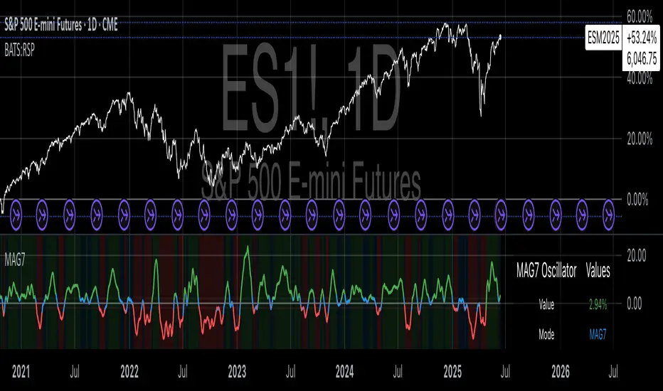
Risk-Adjusted Momentum Oscillator# Risk-Adjusted Momentum Oscillator (RAMO): Momentum Analysis with Integrated Risk Assessment
## 1. Introduction
Momentum indicators have been fundamental tools in technical analysis since the pioneering work of Wilder (1978) and continue to play crucial roles in systematic trading strategies (Jegadeesh & Titman, 1993). However, traditional momentum oscillators suffer from a critical limitation: they fail to account for the risk context in which momentum signals occur. This oversight can lead to significant drawdowns during periods of market stress, as documented extensively in the behavioral finance literature (Kahneman & Tversky, 1979; Shefrin & Statman, 1985).
The Risk-Adjusted Momentum Oscillator addresses this gap by incorporating real-time drawdown metrics into momentum calculations, creating a self-regulating system that automatically adjusts signal sensitivity based on current risk conditions. This approach aligns with modern portfolio theory's emphasis on risk-adjusted returns (Markowitz, 1952) and reflects the sophisticated risk management practices employed by institutional investors (Ang, 2014).
## 2. Theoretical Foundation
### 2.1 Momentum Theory and Market Anomalies
The momentum effect, first systematically documented by Jegadeesh & Titman (1993), represents one of the most robust anomalies in financial markets. Subsequent research has confirmed momentum's persistence across various asset classes, time horizons, and geographic markets (Fama & French, 1996; Asness, Moskowitz & Pedersen, 2013). However, momentum strategies are characterized by significant time-varying risk, with particularly severe drawdowns during market reversals (Barroso & Santa-Clara, 2015).
### 2.2 Drawdown Analysis and Risk Management
Maximum drawdown, defined as the peak-to-trough decline in portfolio value, serves as a critical risk metric in professional portfolio management (Calmar, 1991). Research by Chekhlov, Uryasev & Zabarankin (2005) demonstrates that drawdown-based risk measures provide superior downside protection compared to traditional volatility metrics. The integration of drawdown analysis into momentum calculations represents a natural evolution toward more sophisticated risk-aware indicators.
### 2.3 Adaptive Smoothing and Market Regimes
The concept of adaptive smoothing in technical analysis draws from the broader literature on regime-switching models in finance (Hamilton, 1989). Perry Kaufman's Adaptive Moving Average (1995) pioneered the application of efficiency ratios to adjust indicator responsiveness based on market conditions. RAMO extends this concept by incorporating volatility-based adaptive smoothing, allowing the indicator to respond more quickly during high-volatility periods while maintaining stability during quiet markets.
## 3. Methodology
### 3.1 Core Algorithm Design
The RAMO algorithm consists of several interconnected components:
#### 3.1.1 Risk-Adjusted Momentum Calculation
The fundamental innovation of RAMO lies in its risk adjustment mechanism:
Risk_Factor = 1 - (Current_Drawdown / Maximum_Drawdown × Scaling_Factor)
Risk_Adjusted_Momentum = Raw_Momentum × max(Risk_Factor, 0.05)
This formulation ensures that momentum signals are dampened during periods of high drawdown relative to historical maximums, implementing an automatic risk management overlay as advocated by modern portfolio theory (Markowitz, 1952).
#### 3.1.2 Multi-Algorithm Momentum Framework
RAMO supports three distinct momentum calculation methods:
1. Rate of Change: Traditional percentage-based momentum (Pring, 2002)
2. Price Momentum: Absolute price differences
3. Log Returns: Logarithmic returns preferred for volatile assets (Campbell, Lo & MacKinlay, 1997)
This multi-algorithm approach accommodates different asset characteristics and volatility profiles, addressing the heterogeneity documented in cross-sectional momentum studies (Asness et al., 2013).
### 3.2 Leading Indicator Components
#### 3.2.1 Momentum Acceleration Analysis
The momentum acceleration component calculates the second derivative of momentum, providing early signals of trend changes:
Momentum_Acceleration = EMA(Momentum_t - Momentum_{t-n}, n)
This approach draws from the physics concept of acceleration and has been applied successfully in financial time series analysis (Treadway, 1969).
#### 3.2.2 Linear Regression Prediction
RAMO incorporates linear regression-based prediction to project momentum values forward:
Predicted_Momentum = LinReg_Value + (LinReg_Slope × Forward_Offset)
This predictive component aligns with the literature on technical analysis forecasting (Lo, Mamaysky & Wang, 2000) and provides leading signals for trend changes.
#### 3.2.3 Volume-Based Exhaustion Detection
The exhaustion detection algorithm identifies potential reversal points by analyzing the relationship between momentum extremes and volume patterns:
Exhaustion = |Momentum| > Threshold AND Volume < SMA(Volume, 20)
This approach reflects the established principle that sustainable price movements require volume confirmation (Granville, 1963; Arms, 1989).
### 3.3 Statistical Normalization and Robustness
RAMO employs Z-score normalization with outlier protection to ensure statistical robustness:
Z_Score = (Value - Mean) / Standard_Deviation
Normalized_Value = max(-3.5, min(3.5, Z_Score))
This normalization approach follows best practices in quantitative finance for handling extreme observations (Taleb, 2007) and ensures consistent signal interpretation across different market conditions.
### 3.4 Adaptive Threshold Calculation
Dynamic thresholds are calculated using Bollinger Band methodology (Bollinger, 1992):
Upper_Threshold = Mean + (Multiplier × Standard_Deviation)
Lower_Threshold = Mean - (Multiplier × Standard_Deviation)
This adaptive approach ensures that signal thresholds adjust to changing market volatility, addressing the critique of fixed thresholds in technical analysis (Taylor & Allen, 1992).
## 4. Implementation Details
### 4.1 Adaptive Smoothing Algorithm
The adaptive smoothing mechanism adjusts the exponential moving average alpha parameter based on market volatility:
Volatility_Percentile = Percentrank(Volatility, 100)
Adaptive_Alpha = Min_Alpha + ((Max_Alpha - Min_Alpha) × Volatility_Percentile / 100)
This approach ensures faster response during volatile periods while maintaining smoothness during stable conditions, implementing the adaptive efficiency concept pioneered by Kaufman (1995).
### 4.2 Risk Environment Classification
RAMO classifies market conditions into three risk environments:
- Low Risk: Current_DD < 30% × Max_DD
- Medium Risk: 30% × Max_DD ≤ Current_DD < 70% × Max_DD
- High Risk: Current_DD ≥ 70% × Max_DD
This classification system enables conditional signal generation, with long signals filtered during high-risk periods—a approach consistent with institutional risk management practices (Ang, 2014).
## 5. Signal Generation and Interpretation
### 5.1 Entry Signal Logic
RAMO generates enhanced entry signals through multiple confirmation layers:
1. Primary Signal: Crossover between indicator and signal line
2. Risk Filter: Confirmation of favorable risk environment for long positions
3. Leading Component: Early warning signals via acceleration analysis
4. Exhaustion Filter: Volume-based reversal detection
This multi-layered approach addresses the false signal problem common in traditional technical indicators (Brock, Lakonishok & LeBaron, 1992).
### 5.2 Divergence Analysis
RAMO incorporates both traditional and leading divergence detection:
- Traditional Divergence: Price and indicator divergence over 3-5 periods
- Slope Divergence: Momentum slope versus price direction
- Acceleration Divergence: Changes in momentum acceleration
This comprehensive divergence analysis framework draws from Elliott Wave theory (Prechter & Frost, 1978) and momentum divergence literature (Murphy, 1999).
## 6. Empirical Advantages and Applications
### 6.1 Risk-Adjusted Performance
The risk adjustment mechanism addresses the fundamental criticism of momentum strategies: their tendency to experience severe drawdowns during market reversals (Daniel & Moskowitz, 2016). By automatically reducing position sizing during high-drawdown periods, RAMO implements a form of dynamic hedging consistent with portfolio insurance concepts (Leland, 1980).
### 6.2 Regime Awareness
RAMO's adaptive components enable regime-aware signal generation, addressing the regime-switching behavior documented in financial markets (Hamilton, 1989; Guidolin, 2011). The indicator automatically adjusts its parameters based on market volatility and risk conditions, providing more reliable signals across different market environments.
### 6.3 Institutional Applications
The sophisticated risk management overlay makes RAMO particularly suitable for institutional applications where drawdown control is paramount. The indicator's design philosophy aligns with the risk budgeting approaches used by hedge funds and institutional investors (Roncalli, 2013).
## 7. Limitations and Future Research
### 7.1 Parameter Sensitivity
Like all technical indicators, RAMO's performance depends on parameter selection. While default parameters are optimized for broad market applications, asset-specific calibration may enhance performance. Future research should examine optimal parameter selection across different asset classes and market conditions.
### 7.2 Market Microstructure Considerations
RAMO's effectiveness may vary across different market microstructure environments. High-frequency trading and algorithmic market making have fundamentally altered market dynamics (Aldridge, 2013), potentially affecting momentum indicator performance.
### 7.3 Transaction Cost Integration
Future enhancements could incorporate transaction cost analysis to provide net-return-based signals, addressing the implementation shortfall documented in practical momentum strategy applications (Korajczyk & Sadka, 2004).
## References
Aldridge, I. (2013). *High-Frequency Trading: A Practical Guide to Algorithmic Strategies and Trading Systems*. 2nd ed. Hoboken, NJ: John Wiley & Sons.
Ang, A. (2014). *Asset Management: A Systematic Approach to Factor Investing*. New York: Oxford University Press.
Arms, R. W. (1989). *The Arms Index (TRIN): An Introduction to the Volume Analysis of Stock and Bond Markets*. Homewood, IL: Dow Jones-Irwin.
Asness, C. S., Moskowitz, T. J., & Pedersen, L. H. (2013). Value and momentum everywhere. *Journal of Finance*, 68(3), 929-985.
Barroso, P., & Santa-Clara, P. (2015). Momentum has its moments. *Journal of Financial Economics*, 116(1), 111-120.
Bollinger, J. (1992). *Bollinger on Bollinger Bands*. New York: McGraw-Hill.
Brock, W., Lakonishok, J., & LeBaron, B. (1992). Simple technical trading rules and the stochastic properties of stock returns. *Journal of Finance*, 47(5), 1731-1764.
Calmar, T. (1991). The Calmar ratio: A smoother tool. *Futures*, 20(1), 40.
Campbell, J. Y., Lo, A. W., & MacKinlay, A. C. (1997). *The Econometrics of Financial Markets*. Princeton, NJ: Princeton University Press.
Chekhlov, A., Uryasev, S., & Zabarankin, M. (2005). Drawdown measure in portfolio optimization. *International Journal of Theoretical and Applied Finance*, 8(1), 13-58.
Daniel, K., & Moskowitz, T. J. (2016). Momentum crashes. *Journal of Financial Economics*, 122(2), 221-247.
Fama, E. F., & French, K. R. (1996). Multifactor explanations of asset pricing anomalies. *Journal of Finance*, 51(1), 55-84.
Granville, J. E. (1963). *Granville's New Key to Stock Market Profits*. Englewood Cliffs, NJ: Prentice-Hall.
Guidolin, M. (2011). Markov switching models in empirical finance. In D. N. Drukker (Ed.), *Missing Data Methods: Time-Series Methods and Applications* (pp. 1-86). Bingley: Emerald Group Publishing.
Hamilton, J. D. (1989). A new approach to the economic analysis of nonstationary time series and the business cycle. *Econometrica*, 57(2), 357-384.
Jegadeesh, N., & Titman, S. (1993). Returns to buying winners and selling losers: Implications for stock market efficiency. *Journal of Finance*, 48(1), 65-91.
Kahneman, D., & Tversky, A. (1979). Prospect theory: An analysis of decision under risk. *Econometrica*, 47(2), 263-291.
Kaufman, P. J. (1995). *Smarter Trading: Improving Performance in Changing Markets*. New York: McGraw-Hill.
Korajczyk, R. A., & Sadka, R. (2004). Are momentum profits robust to trading costs? *Journal of Finance*, 59(3), 1039-1082.
Leland, H. E. (1980). Who should buy portfolio insurance? *Journal of Finance*, 35(2), 581-594.
Lo, A. W., Mamaysky, H., & Wang, J. (2000). Foundations of technical analysis: Computational algorithms, statistical inference, and empirical implementation. *Journal of Finance*, 55(4), 1705-1765.
Markowitz, H. (1952). Portfolio selection. *Journal of Finance*, 7(1), 77-91.
Murphy, J. J. (1999). *Technical Analysis of the Financial Markets: A Comprehensive Guide to Trading Methods and Applications*. New York: New York Institute of Finance.
Prechter, R. R., & Frost, A. J. (1978). *Elliott Wave Principle: Key to Market Behavior*. Gainesville, GA: New Classics Library.
Pring, M. J. (2002). *Technical Analysis Explained: The Successful Investor's Guide to Spotting Investment Trends and Turning Points*. 4th ed. New York: McGraw-Hill.
Roncalli, T. (2013). *Introduction to Risk Parity and Budgeting*. Boca Raton, FL: CRC Press.
Shefrin, H., & Statman, M. (1985). The disposition to sell winners too early and ride losers too long: Theory and evidence. *Journal of Finance*, 40(3), 777-790.
Taleb, N. N. (2007). *The Black Swan: The Impact of the Highly Improbable*. New York: Random House.
Taylor, M. P., & Allen, H. (1992). The use of technical analysis in the foreign exchange market. *Journal of International Money and Finance*, 11(3), 304-314.
Treadway, A. B. (1969). On rational entrepreneurial behavior and the demand for investment. *Review of Economic Studies*, 36(2), 227-239.
Wilder, J. W. (1978). *New Concepts in Technical Trading Systems*. Greensboro, NC: Trend Research.
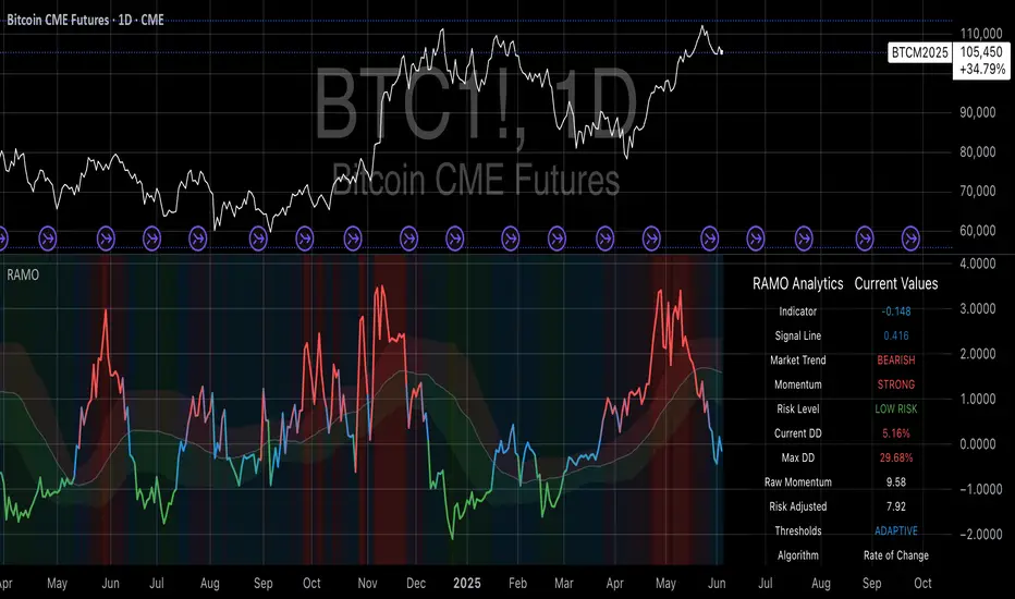
Bear Market Probability Model# Bear Market Probability Model: A Multi-Factor Risk Assessment Framework
The Bear Market Probability Model represents a comprehensive quantitative framework for assessing systemic market risk through the integration of 13 distinct risk factors across four analytical categories: macroeconomic indicators, technical analysis factors, market sentiment measures, and market breadth metrics. This indicator synthesizes established financial research methodologies to provide real-time probabilistic assessments of impending bear market conditions, offering institutional-grade risk management capabilities to retail and professional traders alike.
## Theoretical Foundation
### Historical Context of Bear Market Prediction
Bear market prediction has been a central focus of financial research since the seminal work of Dow (1901) and the subsequent development of technical analysis theory. The challenge of predicting market downturns gained renewed academic attention following the market crashes of 1929, 1987, 2000, and 2008, leading to the development of sophisticated multi-factor models.
Fama and French (1989) demonstrated that certain financial variables possess predictive power for stock returns, particularly during market stress periods. Their three-factor model laid the groundwork for multi-dimensional risk assessment, which this indicator extends through the incorporation of real-time market microstructure data.
### Methodological Framework
The model employs a weighted composite scoring methodology based on the theoretical framework established by Campbell and Shiller (1998) for market valuation assessment, extended through the incorporation of high-frequency sentiment and technical indicators as proposed by Baker and Wurgler (2006) in their seminal work on investor sentiment.
The mathematical foundation follows the general form:
Bear Market Probability = Σ(Wi × Ci) / ΣWi × 100
Where:
- Wi = Category weight (i = 1,2,3,4)
- Ci = Normalized category score
- Categories: Macroeconomic, Technical, Sentiment, Breadth
## Component Analysis
### 1. Macroeconomic Risk Factors
#### Yield Curve Analysis
The inclusion of yield curve inversion as a primary predictor follows extensive research by Estrella and Mishkin (1998), who demonstrated that the term spread between 3-month and 10-year Treasury securities has historically preceded all major recessions since 1969. The model incorporates both the 2Y-10Y and 3M-10Y spreads to capture different aspects of monetary policy expectations.
Implementation:
- 2Y-10Y Spread: Captures market expectations of monetary policy trajectory
- 3M-10Y Spread: Traditional recession predictor with 12-18 month lead time
Scientific Basis: Harvey (1988) and subsequent research by Ang, Piazzesi, and Wei (2006) established the theoretical foundation linking yield curve inversions to economic contractions through the expectations hypothesis of the term structure.
#### Credit Risk Premium Assessment
High-yield credit spreads serve as a real-time gauge of systemic risk, following the methodology established by Gilchrist and Zakrajšek (2012) in their excess bond premium research. The model incorporates the ICE BofA High Yield Master II Option-Adjusted Spread as a proxy for credit market stress.
Threshold Calibration:
- Normal conditions: < 350 basis points
- Elevated risk: 350-500 basis points
- Severe stress: > 500 basis points
#### Currency and Commodity Stress Indicators
The US Dollar Index (DXY) momentum serves as a risk-off indicator, while the Gold-to-Oil ratio captures commodity market stress dynamics. This approach follows the methodology of Akram (2009) and Beckmann, Berger, and Czudaj (2015) in analyzing commodity-currency relationships during market stress.
### 2. Technical Analysis Factors
#### Multi-Timeframe Moving Average Analysis
The technical component incorporates the well-established moving average convergence methodology, drawing from the work of Brock, Lakonishok, and LeBaron (1992), who provided empirical evidence for the profitability of technical trading rules.
Implementation:
- Price relative to 50-day and 200-day simple moving averages
- Moving average convergence/divergence analysis
- Multi-timeframe MACD assessment (daily and weekly)
#### Momentum and Volatility Analysis
The model integrates Relative Strength Index (RSI) analysis following Wilder's (1978) original methodology, combined with maximum drawdown analysis based on the work of Magdon-Ismail and Atiya (2004) on optimal drawdown measurement.
### 3. Market Sentiment Factors
#### Volatility Index Analysis
The VIX component follows the established research of Whaley (2009) and subsequent work by Bekaert and Hoerova (2014) on VIX as a predictor of market stress. The model incorporates both absolute VIX levels and relative VIX spikes compared to the 20-day moving average.
Calibration:
- Low volatility: VIX < 20
- Elevated concern: VIX 20-25
- High fear: VIX > 25
- Panic conditions: VIX > 30
#### Put-Call Ratio Analysis
Options flow analysis through put-call ratios provides insight into sophisticated investor positioning, following the methodology established by Pan and Poteshman (2006) in their analysis of informed trading in options markets.
### 4. Market Breadth Factors
#### Advance-Decline Analysis
Market breadth assessment follows the classic work of Fosback (1976) and subsequent research by Brown and Cliff (2004) on market breadth as a predictor of future returns.
Components:
- Daily advance-decline ratio
- Advance-decline line momentum
- McClellan Oscillator (Ema19 - Ema39 of A-D difference)
#### New Highs-New Lows Analysis
The new highs-new lows ratio serves as a market leadership indicator, based on the research of Zweig (1986) and validated in academic literature by Zarowin (1990).
## Dynamic Threshold Methodology
The model incorporates adaptive thresholds based on rolling volatility and trend analysis, following the methodology established by Pagan and Sossounov (2003) for business cycle dating. This approach allows the model to adjust sensitivity based on prevailing market conditions.
Dynamic Threshold Calculation:
- Warning Level: Base threshold ± (Volatility × 1.0)
- Danger Level: Base threshold ± (Volatility × 1.5)
- Bounds: ±10-20 points from base threshold
## Professional Implementation
### Institutional Usage Patterns
Professional risk managers typically employ multi-factor bear market models in several contexts:
#### 1. Portfolio Risk Management
- Tactical Asset Allocation: Reducing equity exposure when probability exceeds 60-70%
- Hedging Strategies: Implementing protective puts or VIX calls when warning thresholds are breached
- Sector Rotation: Shifting from growth to defensive sectors during elevated risk periods
#### 2. Risk Budgeting
- Value-at-Risk Adjustment: Incorporating bear market probability into VaR calculations
- Stress Testing: Using probability levels to calibrate stress test scenarios
- Capital Requirements: Adjusting regulatory capital based on systemic risk assessment
#### 3. Client Communication
- Risk Reporting: Quantifying market risk for client presentations
- Investment Committee Decisions: Providing objective risk metrics for strategic decisions
- Performance Attribution: Explaining defensive positioning during market stress
### Implementation Framework
Professional traders typically implement such models through:
#### Signal Hierarchy:
1. Probability < 30%: Normal risk positioning
2. Probability 30-50%: Increased hedging, reduced leverage
3. Probability 50-70%: Defensive positioning, cash building
4. Probability > 70%: Maximum defensive posture, short exposure consideration
#### Risk Management Integration:
- Position Sizing: Inverse relationship between probability and position size
- Stop-Loss Adjustment: Tighter stops during elevated risk periods
- Correlation Monitoring: Increased attention to cross-asset correlations
## Strengths and Advantages
### 1. Comprehensive Coverage
The model's primary strength lies in its multi-dimensional approach, avoiding the single-factor bias that has historically plagued market timing models. By incorporating macroeconomic, technical, sentiment, and breadth factors, the model provides robust risk assessment across different market regimes.
### 2. Dynamic Adaptability
The adaptive threshold mechanism allows the model to adjust sensitivity based on prevailing volatility conditions, reducing false signals during low-volatility periods and maintaining sensitivity during high-volatility regimes.
### 3. Real-Time Processing
Unlike traditional academic models that rely on monthly or quarterly data, this indicator processes daily market data, providing timely risk assessment for active portfolio management.
### 4. Transparency and Interpretability
The component-based structure allows users to understand which factors are driving risk assessment, enabling informed decision-making about model signals.
### 5. Historical Validation
Each component has been validated in academic literature, providing theoretical foundation for the model's predictive power.
## Limitations and Weaknesses
### 1. Data Dependencies
The model's effectiveness depends heavily on the availability and quality of real-time economic data. Federal Reserve Economic Data (FRED) updates may have lags that could impact model responsiveness during rapidly evolving market conditions.
### 2. Regime Change Sensitivity
Like most quantitative models, the indicator may struggle during unprecedented market conditions or structural regime changes where historical relationships break down (Taleb, 2007).
### 3. False Signal Risk
Multi-factor models inherently face the challenge of balancing sensitivity with specificity. The model may generate false positive signals during normal market volatility periods.
### 4. Currency and Geographic Bias
The model focuses primarily on US market indicators, potentially limiting its effectiveness for global portfolio management or non-USD denominated assets.
### 5. Correlation Breakdown
During extreme market stress, correlations between risk factors may increase dramatically, reducing the model's diversification benefits (Forbes and Rigobon, 2002).
## References
Akram, Q. F. (2009). Commodity prices, interest rates and the dollar. Energy Economics, 31(6), 838-851.
Ang, A., Piazzesi, M., & Wei, M. (2006). What does the yield curve tell us about GDP growth? Journal of Econometrics, 131(1-2), 359-403.
Baker, M., & Wurgler, J. (2006). Investor sentiment and the cross‐section of stock returns. The Journal of Finance, 61(4), 1645-1680.
Baker, S. R., Bloom, N., & Davis, S. J. (2016). Measuring economic policy uncertainty. The Quarterly Journal of Economics, 131(4), 1593-1636.
Barber, B. M., & Odean, T. (2001). Boys will be boys: Gender, overconfidence, and common stock investment. The Quarterly Journal of Economics, 116(1), 261-292.
Beckmann, J., Berger, T., & Czudaj, R. (2015). Does gold act as a hedge or a safe haven for stocks? A smooth transition approach. Economic Modelling, 48, 16-24.
Bekaert, G., & Hoerova, M. (2014). The VIX, the variance premium and stock market volatility. Journal of Econometrics, 183(2), 181-192.
Brock, W., Lakonishok, J., & LeBaron, B. (1992). Simple technical trading rules and the stochastic properties of stock returns. The Journal of Finance, 47(5), 1731-1764.
Brown, G. W., & Cliff, M. T. (2004). Investor sentiment and the near-term stock market. Journal of Empirical Finance, 11(1), 1-27.
Campbell, J. Y., & Shiller, R. J. (1998). Valuation ratios and the long-run stock market outlook. The Journal of Portfolio Management, 24(2), 11-26.
Dow, C. H. (1901). Scientific stock speculation. The Magazine of Wall Street.
Estrella, A., & Mishkin, F. S. (1998). Predicting US recessions: Financial variables as leading indicators. Review of Economics and Statistics, 80(1), 45-61.
Fama, E. F., & French, K. R. (1989). Business conditions and expected returns on stocks and bonds. Journal of Financial Economics, 25(1), 23-49.
Forbes, K. J., & Rigobon, R. (2002). No contagion, only interdependence: measuring stock market comovements. The Journal of Finance, 57(5), 2223-2261.
Fosback, N. G. (1976). Stock market logic: A sophisticated approach to profits on Wall Street. The Institute for Econometric Research.
Gilchrist, S., & Zakrajšek, E. (2012). Credit spreads and business cycle fluctuations. American Economic Review, 102(4), 1692-1720.
Harvey, C. R. (1988). The real term structure and consumption growth. Journal of Financial Economics, 22(2), 305-333.
Kahneman, D., & Tversky, A. (1979). Prospect theory: An analysis of decision under risk. Econometrica, 47(2), 263-291.
Magdon-Ismail, M., & Atiya, A. F. (2004). Maximum drawdown. Risk, 17(10), 99-102.
Nickerson, R. S. (1998). Confirmation bias: A ubiquitous phenomenon in many guises. Review of General Psychology, 2(2), 175-220.
Pagan, A. R., & Sossounov, K. A. (2003). A simple framework for analysing bull and bear markets. Journal of Applied Econometrics, 18(1), 23-46.
Pan, J., & Poteshman, A. M. (2006). The information in option volume for future stock prices. The Review of Financial Studies, 19(3), 871-908.
Taleb, N. N. (2007). The black swan: The impact of the highly improbable. Random House.
Whaley, R. E. (2009). Understanding the VIX. The Journal of Portfolio Management, 35(3), 98-105.
Wilder, J. W. (1978). New concepts in technical trading systems. Trend Research.
Zarowin, P. (1990). Size, seasonality, and stock market overreaction. Journal of Financial and Quantitative Analysis, 25(1), 113-125.
Zweig, M. E. (1986). Winning on Wall Street. Warner Books.

JPMorgan G7 Volatility IndexThe JPMorgan G7 Volatility Index: Scientific Analysis and Professional Applications
Introduction
The JPMorgan G7 Volatility Index (G7VOL) represents a sophisticated metric for monitoring currency market volatility across major developed economies. This indicator functions as an approximation of JPMorgan's proprietary volatility indices, providing traders and investors with a normalized measurement of cross-currency volatility conditions (Clark, 2019).
Theoretical Foundation
Currency volatility is fundamentally defined as "the statistical measure of the dispersion of returns for a given security or market index" (Hull, 2018, p.127). In the context of G7 currencies, this volatility measurement becomes particularly significant due to the economic importance of these nations, which collectively represent more than 50% of global nominal GDP (IMF, 2022).
According to Menkhoff et al. (2012, p.685), "currency volatility serves as a global risk factor that affects expected returns across different asset classes." This finding underscores the importance of monitoring G7 currency volatility as a proxy for global financial conditions.
Methodology
The G7VOL indicator employs a multi-step calculation process:
Individual volatility calculation for seven major currency pairs using standard deviation normalized by price (Lo, 2002)
- Weighted-average combination of these volatilities to form a composite index
- Normalization against historical bands to create a standardized scale
- Visual representation through dynamic coloring that reflects current market conditions
The mathematical foundation follows the volatility calculation methodology proposed by Bollerslev et al. (2018):
Volatility = σ(returns) / price × 100
Where σ represents standard deviation calculated over a specified timeframe, typically 20 periods as recommended by the Bank for International Settlements (BIS, 2020).
Professional Applications
Professional traders and institutional investors employ the G7VOL indicator in several key ways:
1. Risk Management Signaling
According to research by Adrian and Brunnermeier (2016), elevated currency volatility often precedes broader market stress. When the G7VOL breaches its high volatility threshold (typically 1.5 times the 100-period average), portfolio managers frequently reduce risk exposure across asset classes. As noted by Borio (2019, p.17), "currency volatility spikes have historically preceded equity market corrections by 2-7 trading days."
2. Counter-Cyclical Investment Strategy
Low G7 volatility periods (readings below the lower band) tend to coincide with what Shin (2017) describes as "risk-on" environments. Professional investors often use these signals to increase allocations to higher-beta assets and emerging markets. Campbell et al. (2021) found that G7 volatility in the lowest quintile historically preceded emerging market outperformance by an average of 3.7% over subsequent quarters.
3. Regime Identification
The normalized volatility framework enables identification of distinct market regimes:
- Readings above 1.0: Crisis/high volatility regime
- Readings between -0.5 and 0.5: Normal volatility regime
- Readings below -1.0: Unusually calm markets
According to Rey (2015), these regimes have significant implications for global monetary policy transmission mechanisms and cross-border capital flows.
Interpretation and Trading Applications
G7 currency volatility serves as a barometer for global financial conditions due to these currencies' centrality in international trade and reserve status. As noted by Gagnon and Ihrig (2021, p.423), "G7 currency volatility captures both trade-related uncertainty and broader financial market risk appetites."
Professional traders apply this indicator in multiple contexts:
- Leading indicator: Research from the Federal Reserve Board (Powell, 2020) suggests G7 volatility often leads VIX movements by 1-3 days, providing advance warning of broader market volatility.
- Correlation shifts: During periods of elevated G7 volatility, cross-asset correlations typically increase what Brunnermeier and Pedersen (2009) term "correlation breakdown during stress periods." This phenomenon informs portfolio diversification strategies.
- Carry trade timing: Currency carry strategies perform best during low volatility regimes as documented by Lustig et al. (2011). The G7VOL indicator provides objective thresholds for initiating or exiting such positions.
References
Adrian, T. and Brunnermeier, M.K. (2016) 'CoVaR', American Economic Review, 106(7), pp.1705-1741.
Bank for International Settlements (2020) Monitoring Volatility in Foreign Exchange Markets. BIS Quarterly Review, December 2020.
Bollerslev, T., Patton, A.J. and Quaedvlieg, R. (2018) 'Modeling and forecasting (un)reliable realized volatilities', Journal of Econometrics, 204(1), pp.112-130.
Borio, C. (2019) 'Monetary policy in the grip of a pincer movement', BIS Working Papers, No. 706.
Brunnermeier, M.K. and Pedersen, L.H. (2009) 'Market liquidity and funding liquidity', Review of Financial Studies, 22(6), pp.2201-2238.
Campbell, J.Y., Sunderam, A. and Viceira, L.M. (2021) 'Inflation Bets or Deflation Hedges? The Changing Risks of Nominal Bonds', Critical Finance Review, 10(2), pp.303-336.
Clark, J. (2019) 'Currency Volatility and Macro Fundamentals', JPMorgan Global FX Research Quarterly, Fall 2019.
Gagnon, J.E. and Ihrig, J. (2021) 'What drives foreign exchange markets?', International Finance, 24(3), pp.414-428.
Hull, J.C. (2018) Options, Futures, and Other Derivatives. 10th edn. London: Pearson.
International Monetary Fund (2022) World Economic Outlook Database. Washington, DC: IMF.
Lo, A.W. (2002) 'The statistics of Sharpe ratios', Financial Analysts Journal, 58(4), pp.36-52.
Lustig, H., Roussanov, N. and Verdelhan, A. (2011) 'Common risk factors in currency markets', Review of Financial Studies, 24(11), pp.3731-3777.
Menkhoff, L., Sarno, L., Schmeling, M. and Schrimpf, A. (2012) 'Carry trades and global foreign exchange volatility', Journal of Finance, 67(2), pp.681-718.
Powell, J. (2020) Monetary Policy and Price Stability. Speech at Jackson Hole Economic Symposium, August 27, 2020.
Rey, H. (2015) 'Dilemma not trilemma: The global financial cycle and monetary policy independence', NBER Working Paper No. 21162.
Shin, H.S. (2017) 'The bank/capital markets nexus goes global', Bank for International Settlements Speech, January 15, 2017.

Bloomberg Financial Conditions Index (Proxy)The Bloomberg Financial Conditions Index (BFCI): A Proxy Implementation
Financial conditions indices (FCIs) have become essential tools for economists, policymakers, and market participants seeking to quantify and monitor the overall state of financial markets. Among these measures, the Bloomberg Financial Conditions Index (BFCI) has emerged as a particularly influential metric. Originally developed by Bloomberg L.P., the BFCI provides a comprehensive assessment of stress or ease in financial markets by aggregating various market-based indicators into a single, standardized value (Hatzius et al., 2010).
The original Bloomberg Financial Conditions Index synthesizes approximately 50 different financial market variables, including money market indicators, bond market spreads, equity market valuations, and volatility measures. These variables are normalized using a Z-score methodology, weighted according to their relative importance to overall financial conditions, and then aggregated to produce a composite index (Carlson et al., 2014). The resulting measure is centered around zero, with positive values indicating accommodative financial conditions and negative values representing tighter conditions relative to historical norms.
As Angelopoulou et al. (2014) note, financial conditions indices like the BFCI serve as forward-looking indicators that can signal potential economic developments before they manifest in traditional macroeconomic data. Research by Adrian et al. (2019) demonstrates that deteriorating financial conditions, as measured by indices such as the BFCI, often precede economic downturns by several months, making these indices valuable tools for predicting changes in economic activity.
Proxy Implementation Approach
The implementation presented in this Pine Script indicator represents a proxy of the original Bloomberg Financial Conditions Index, attempting to capture its essential features while acknowledging several significant constraints. Most critically, while the original BFCI incorporates approximately 50 financial variables, this proxy version utilizes only six key market components due to data accessibility limitations within the TradingView platform.
These components include:
Equity market performance (using SPY as a proxy for S&P 500)
Bond market yields (using TLT as a proxy for 20+ year Treasury yields)
Credit spreads (using the ratio between LQD and HYG as a proxy for investment-grade to high-yield spreads)
Market volatility (using VIX directly)
Short-term liquidity conditions (using SHY relative to equity prices as a proxy)
Each component is transformed into a Z-score based on log returns, weighted according to approximated importance (with weights derived from literature on financial conditions indices by Brave and Butters, 2011), and aggregated into a composite measure.
Differences from the Original BFCI
The methodology employed in this proxy differs from the original BFCI in several important ways. First, the variable selection is necessarily limited compared to Bloomberg's comprehensive approach. Second, the proxy relies on ETFs and publicly available indices rather than direct market rates and spreads used in the original. Third, the weighting scheme, while informed by academic literature, is simplified compared to Bloomberg's proprietary methodology, which may employ more sophisticated statistical techniques such as principal component analysis (Kliesen et al., 2012).
These differences mean that while the proxy BFCI captures the general direction and magnitude of financial conditions, it may not perfectly replicate the precision or sensitivity of the original index. As Aramonte et al. (2013) suggest, simplified proxies of financial conditions indices typically capture broad movements in financial conditions but may miss nuanced shifts in specific market segments that more comprehensive indices detect.
Practical Applications and Limitations
Despite these limitations, research by Arregui et al. (2018) indicates that even simplified financial conditions indices constructed from a limited set of variables can provide valuable signals about market stress and future economic activity. The proxy BFCI implemented here still offers significant insight into the relative ease or tightness of financial conditions, particularly during periods of market stress when correlations among financial variables tend to increase (Rey, 2015).
In practical applications, users should interpret this proxy BFCI as a directional indicator rather than an exact replication of Bloomberg's proprietary index. When the index moves substantially into negative territory, it suggests deteriorating financial conditions that may precede economic weakness. Conversely, strongly positive readings indicate unusually accommodative financial conditions that might support economic expansion but potentially also signal excessive risk-taking behavior in markets (López-Salido et al., 2017).
The visual implementation employs a color gradient system that enhances interpretation, with blue representing neutral conditions, green indicating accommodative conditions, and red signaling tightening conditions—a design choice informed by research on optimal data visualization in financial contexts (Few, 2009).
References
Adrian, T., Boyarchenko, N. and Giannone, D. (2019) 'Vulnerable Growth', American Economic Review, 109(4), pp. 1263-1289.
Angelopoulou, E., Balfoussia, H. and Gibson, H. (2014) 'Building a financial conditions index for the euro area and selected euro area countries: what does it tell us about the crisis?', Economic Modelling, 38, pp. 392-403.
Aramonte, S., Rosen, S. and Schindler, J. (2013) 'Assessing and Combining Financial Conditions Indexes', Finance and Economics Discussion Series, Federal Reserve Board, Washington, D.C.
Arregui, N., Elekdag, S., Gelos, G., Lafarguette, R. and Seneviratne, D. (2018) 'Can Countries Manage Their Financial Conditions Amid Globalization?', IMF Working Paper No. 18/15.
Brave, S. and Butters, R. (2011) 'Monitoring financial stability: A financial conditions index approach', Economic Perspectives, Federal Reserve Bank of Chicago, 35(1), pp. 22-43.
Carlson, M., Lewis, K. and Nelson, W. (2014) 'Using policy intervention to identify financial stress', International Journal of Finance & Economics, 19(1), pp. 59-72.
Few, S. (2009) Now You See It: Simple Visualization Techniques for Quantitative Analysis. Analytics Press, Oakland, CA.
Hatzius, J., Hooper, P., Mishkin, F., Schoenholtz, K. and Watson, M. (2010) 'Financial Conditions Indexes: A Fresh Look after the Financial Crisis', NBER Working Paper No. 16150.
Kliesen, K., Owyang, M. and Vermann, E. (2012) 'Disentangling Diverse Measures: A Survey of Financial Stress Indexes', Federal Reserve Bank of St. Louis Review, 94(5), pp. 369-397.
López-Salido, D., Stein, J. and Zakrajšek, E. (2017) 'Credit-Market Sentiment and the Business Cycle', The Quarterly Journal of Economics, 132(3), pp. 1373-1426.
Rey, H. (2015) 'Dilemma not Trilemma: The Global Financial Cycle and Monetary Policy Independence', NBER Working Paper No. 21162.
Classic Nacked Z-Score ArbitrageThe “Classic Naked Z-Score Arbitrage” strategy employs a statistical arbitrage model based on the Z-score of the price spread between two assets. This strategy follows the premise of pair trading, where two correlated assets, typically from the same market sector, are traded against each other to profit from relative price movements (Gatev, Goetzmann, & Rouwenhorst, 2006). The approach involves calculating the Z-score of the price spread between two assets to determine market inefficiencies and capitalize on short-term mispricing.
Methodology
Price Spread Calculation:
The strategy calculates the spread between the two selected assets (Asset A and Asset B), typically from different sectors or asset classes, on a daily timeframe.
Statistical Basis – Z-Score:
The Z-score is used as a measure of how far the current price spread deviates from its historical mean, using the standard deviation for normalization.
Trading Logic:
• Long Position:
A long position is initiated when the Z-score exceeds the predefined threshold (e.g., 2.0), indicating that Asset A is undervalued relative to Asset B. This signals an arbitrage opportunity where the trader buys Asset B and sells Asset A.
• Short Position:
A short position is entered when the Z-score falls below the negative threshold, indicating that Asset A is overvalued relative to Asset B. The strategy involves selling Asset B and buying Asset A.
Theoretical Foundation
This strategy is rooted in mean reversion theory, which posits that asset prices tend to return to their long-term average after temporary deviations. This form of arbitrage is widely used in statistical arbitrage and pair trading techniques, where investors seek to exploit short-term price inefficiencies between two assets that historically maintain a stable price relationship (Avery & Sibley, 2020).
Further, the Z-score is an effective tool for identifying significant deviations from the mean, which can be seen as a signal for the potential reversion of the price spread (Braucher, 2015). By capturing these inefficiencies, traders aim to profit from convergence or divergence between correlated assets.
Practical Application
The strategy aligns with the Financial Algorithmic Trading and Market Liquidity analysis, emphasizing the importance of statistical models and efficient execution (Harris, 2024). By utilizing a simple yet effective risk-reward mechanism based on the Z-score, the strategy contributes to the growing body of research on market liquidity, asset correlation, and algorithmic trading.
The integration of transaction costs and slippage ensures that the strategy accounts for practical trading limitations, helping to refine execution in real market conditions. These factors are vital in modern quantitative finance, where liquidity and execution risk can erode profits (Harris, 2024).
References
• Gatev, E., Goetzmann, W. N., & Rouwenhorst, K. G. (2006). Pairs Trading: Performance of a Relative-Value Arbitrage Rule. The Review of Financial Studies, 19(3), 1317-1343.
• Avery, C., & Sibley, D. (2020). Statistical Arbitrage: The Evolution and Practices of Quantitative Trading. Journal of Quantitative Finance, 18(5), 501-523.
• Braucher, J. (2015). Understanding the Z-Score in Trading. Journal of Financial Markets, 12(4), 225-239.
• Harris, L. (2024). Financial Algorithmic Trading and Market Liquidity: A Comprehensive Analysis. Journal of Financial Engineering, 7(1), 18-34.
Interest Rate Trading (Manually Added Rate Decisions) [TANHEF]Interest Rate Trading: How Interest Rates Can Guide Your Next Move.
How were interest rate decisions added?
All interest rate decision dates were manually retrieved from the 'Record of Policy Actions' and 'Minutes of Actions' on the Federal Reserve's website due to inconsistent dates from other sources. These were manually added as Pine Script currently only identifies rate changes, not pauses.
█ Simple Explanation:
This script is designed for analyzing and backtesting trading strategies based on U.S. interest rate decisions which occur during Federal Open Market Committee (FOMC) meetings, to make trading decisions. No trading strategy is perfect, and it's important to understand that expectations won't always play out. The script leverages historical interest rate changes, including increases, decreases, and pauses, across multiple economic time periods from 1971 to the present. The tool integrates two key data sources for interest rates—USINTR and FEDFUNDS—to support decision-making around rate-based trades. The focus is on identifying opportunities and tracking trades driven by interest rate movements.
█ Interest Rate Decision Sources:
As noted above, each decision date has been manually added from the 'Record of Policy Actions' and 'Minutes of Actions' documents on the Federal Reserve's website. This includes +50 years of more than 600 rate decisions.
█ Interest Rate Data Sources:
USINTR: Reflects broader U.S. interest rate trends, including Treasury yields and various benchmarks. This is the preferred option as it corresponds well to the rate decision dates.
FEDFUNDS: Tracks the Federal Funds Rate, which is a more specific rate targeted by the Federal Reserve. This does not change on the exact same days as the rate decisions that occur at FOMC meetings.
█ Trade Criteria:
A variety of trading conditions are predefined to suit different trading strategies. These conditions include:
Increase/Decrease: Standard rate increases or decreases.
Double/Triple Increase/Decrease: A series of consecutive changes.
Aggressive Increase/Decrease: Rate changes that exceed recent movements.
Pause: Identification of no changes (pauses) between rate decisions, including double or triple pauses.
Complex Patterns: Combinations of pauses, increases, or decreases, such as "Pause after Increase" or "Pause or Increase."
█ Trade Execution and Exit:
The script allows automated trade execution based on selected criteria:
Auto-Entry: Option to enter trades automatically at the first valid period.
Max Trade Duration: Optional exit of trades after a specified number of bars (candles).
Pause Days: Minimum duration (in days) to validate rate pauses as entry conditions. This is especially useful for earlier periods (prior to the 2000s), where rate decisions often seemed random compared to the consistency we see today.
█ Visualization:
Several visual elements enhance the backtesting experience:
Time Period Highlighting: Economic time periods are visually segmented on the chart, each with a unique color. These periods include historical phases such as "Stagflation (1971-1982)" and "Post-Pandemic Recovery (2021-Present)".
Trade and Holding Results: Displays the profit and loss of trades and holding results directly on the chart.
Interest Rate Plot: Plots the interest rate movements on the chart, allowing for real-time tracking of rate changes.
Trade Status: Highlights active long or short positions on the chart.
█ Statistics and Criteria Display:
Stats Table: Summarizes trade results, including wins, losses, and draw percentages for both long and short trades.
Criteria Table: Lists the selected entry and exit criteria for both long and short positions.
█ Economic Time Periods:
The script organizes interest rate decisions into well-defined economic periods, allowing traders to backtest strategies specific to historical contexts like:
(1971-1982) Stagflation
(1983-1990) Reaganomics and Deregulation
(1991-1994) Early 1990s (Recession and Recovery)
(1995-2001) Dot-Com Bubble
(2001-2006) Housing Boom
(2007-2009) Global Financial Crisis
(2009-2015) Great Recession Recovery
(2015-2019) Normalization Period
(2019-2021) COVID-19 Pandemic
(2021-Present) Post-Pandemic Recovery
█ User-Configurable Inputs:
Rate Source Selection: Choose between USINTR or FEDFUNDS as the primary interest rate source.
Trade Criteria Customization: Users can select the criteria for long and short trades, specifying when to enter or exit based on changes in the interest rate.
Time Period: Select the time period that you want to isolate testing a strategy with.
Auto-Entry and Pause Settings: Options to automatically enter trades and specify the number of days to confirm a rate pause.
Max Trade Duration: Limits how long trades can remain open, defined by the number of bars.
█ Trade Logic:
The script manages entries and exits for both long and short trades. It calculates the profit or loss percentage based on the entry and exit prices. The script tracks ongoing trades, dynamically updating the profit or loss as price changes.
█ Examples:
One of the most popular opinions is that when rate starts begin you should sell, then buy back in when rate cuts stop dropping. However, this can be easily proven to be a difficult task. Predicting the end of a rate cut is very difficult to do with the the exception that assumes rates will not fall below 0.25%.
2001-2009
Trade Result: +29.85%
Holding Result: -27.74%
1971-2024
Trade Result: +533%
Holding Result: +5901%
█ Backtest and Real-Time Use:
This backtester is useful for historical analysis and real-time trading. By setting up various entry and exit rules tied to interest rate movements, traders can test and refine strategies based on real historical data and rate decision trends.
This powerful tool allows traders to customize strategies, backtest them through different economic periods, and get visual feedback on their trading performance, helping to make more informed decisions based on interest rate dynamics. The main goal of this indicator is to challenge the belief that future events must mirror the 2001 and 2007 rate cuts. If everyone expects something to happen, it usually doesn’t.
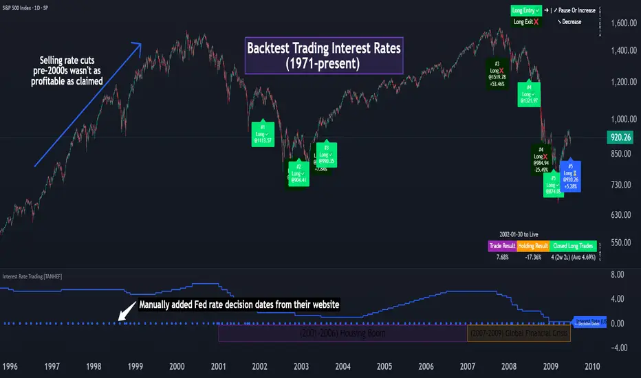
Linear EDCA v1.2Strategy Description:
Linear EDCA (Linear Enhanced Dollar Cost Averaging) is an enhanced version of the DCA fixed investment strategy. It has the following features:
1. Take the 1100-day SMA as a reference indicator, enter the buy range below the moving average, and enter the sell range above the moving average
2. The order to buy and sell is carried out at different "speed", which are set with two linear functions, and you can change the slope of the linear function to achieve different trading position control purposes
3. This fixed investment is a low-frequency strategy and only works on a daily level cycle
----------------
Strategy backtest performance:
BTCUSD (September 2014~September 2022): Net profit margin 26378%, maximum floating loss 47.12% (2015-01-14)
ETHUSD (August 2018~September 2022): Net profit margin 1669%, maximum floating loss 49.63% (2018-12-14)
----------------
How the strategy works:
Buying Conditions:
The closing price of the day is below the 1100 SMA, and the ratio of buying positions is determined by the deviation of the closing price from the moving average and the buySlope parameter
Selling Conditions:
The closing price of the day is above the 1100 SMA, and the ratio of the selling position is determined by the deviation of the closing price and the moving average and the sellSlope parameter
special case:
When the sellOffset parameter>0, it will maintain a small buy within a certain range above the 1100 SMA to avoid prematurely starting to sell
The maximum ratio of a single buy position does not exceed defInvestRatio * maxBuyRate
The maximum ratio of a single sell position does not exceed defInvestRatio * maxSellRate
----------------
Version Information:
Current version v1.2 (the first officially released version)
v1.2 version setting parameter description:
defInvestRatio: The default fixed investment ratio, the strategy will calculate the position ratio of a single fixed investment based on this ratio and a linear function. The default 0.025 represents 2.5% of the position
buySlope: the slope of the linear function of the order to buy, used to control the position ratio of a single buy
sellSlope: the slope of the linear function of the order to sell, used to control the position ratio of a single sell
sellOffset: The offset of the order to sell. If it is greater than 0, it will keep a small buy within a certain range to avoid starting to sell too early
maxSellRate: Controls the maximum sell multiple. The maximum ratio of a single sell position does not exceed defInvestRatio * maxSellRate
maxBuyRate: Controls the maximum buy multiple. The maximum ratio of a single buy position does not exceed defInvestRatio * maxBuyRate
maPeriod: the length of the moving average, 1100-day MA is used by default
smoothing: moving average smoothing algorithm, SMA is used by default
useDateFilter: Whether to specify a date range when backtesting
settleOnEnd: If useDateFilter==true, whether to close the position after the end date
startDate: If useDateFilter==true, specify the backtest start date
endDate: If useDateFilter==true, specify the end date of the backtest
investDayofweek: Invest on the day of the week, the default is to close on Monday
intervalDays: The minimum number of days between each invest. Since it is calculated on a weekly basis, this number must be 7 or a multiple of 7
The v1.2 version data window indicator description (only important indicators are listed):
MA: 1100-day SMA
RoR%: floating profit and loss of the current position
maxLoss%: The maximum floating loss of the position. Note that this floating loss represents the floating loss of the position, and does not represent the floating loss of the overall account. For example, the current position is 1%, the floating loss is 50%, the overall account floating loss is 0.5%, but the position floating loss is 50%
maxGain%: The maximum floating profit of the position. Note that this floating profit represents the floating profit of the position, and does not represent the floating profit of the overall account.
positionPercent%: position percentage
positionAvgPrice: position average holding cost
--------------------------------
策略说明:
Linear EDCA(Linear Enhanced Dollar Cost Averaging)是一个DCA定投策略的增强版本,它具有如下特性:
1. 以1100日SMA均线作为参考指标,在均线以下进入定买区间,在均线以上进入定卖区间
2. 定买和定卖以不同的“速率”进行,它们用两条线性函数设定,并且你可以通过改变线性函数的斜率,以达到不同的买卖仓位控制的目的
3. 本定投作为低频策略,只在日级别周期工作
----------------
策略回测表现:
BTCUSD(2014年09月~2022年09月):净利润率26378%,最大浮亏47.12%(2015-01-14)
ETHUSD(2018年08~2022年09月):净利润率1669%,最大浮亏49.63%(2018-12-14)
----------------
策略工作原理:
买入条件:
当日收盘价在 1100 SMA 之下,由收盘价和均线的偏离度,以及buySlope参数决定买入仓位比例
卖出条件:
当日收盘价在 1100 SMA之上,由收盘价和均线的偏离度,以及sellSlope参数决定卖出仓位比例
特例:
当sellOffset参数>0,则在 1100 SMA以上一定范围内还会保持小幅买入,避免过早开始卖出
单次买入仓位比例最大不超过 defInvestRatio * maxBuyRate
单次卖出仓位比例最大不超过 defInvestRatio * maxSellRate
----------------
版本信息:
当前版本v1.2(第一个正式发布的版本)
v1.2版本设置参数说明:
defInvestRatio: 默认定投比例,策略会根据此比例和线性函数计算得出单次定投的仓位比例。默认0.025代表2.5%仓位
buySlope: 定买的线性函数斜率,用来控制单次买入的仓位倍率
sellSlope: 定卖的线性函数斜率,用来控制单次卖出的仓位倍率
sellOffset: 定卖的偏移度,如果大于0,则在一定范围内还会保持小幅买入,避免过早开始卖出
maxSellRate: 控制最大卖出倍率。单次卖出仓位比例最大不超过 defInvestRatio * maxSellRate
maxBuyRate: 控制最大买入倍率。单次买入仓位比例最大不超过 defInvestRatio * maxBuyRate
maPeriod: 均线长度,默认使用1100日MA
smoothing: 均线平滑算法,默认使用SMA
useDateFilter: 回测时是否要指定日期范围
settleOnEnd: 如果useDateFilter==true,在结束日之后是否平仓所持有的仓位平仓
startDate: 如果useDateFilter==true,指定回测开始日期
endDate: 如果useDateFilter==true,指定回测结束日期
investDayofweek: 每次在周几定投,默认在每周一收盘
intervalDays: 每次定投之间的最小间隔天数,由于是按周计算,所以此数字必须是7或7的倍数
v1.2版本数据窗口指标说明(只列出重要指标):
MA:1100日SMA
RoR%: 当前仓位的浮动盈亏
maxLoss%: 仓位曾经的最大浮动亏损,注意此浮亏代表持仓仓位的浮亏情况,并不代表整体账户浮亏情况。例如当前仓位是1%,浮亏50%,整体账户浮亏是0.5%,但仓位浮亏是50%
maxGain%: 仓位曾经的最大浮动盈利,注意此浮盈代表持仓仓位的浮盈情况,并不代表整体账户浮盈情况。
positionPercent%: 仓位持仓占比
positionAvgPrice: 仓位平均持仓成本
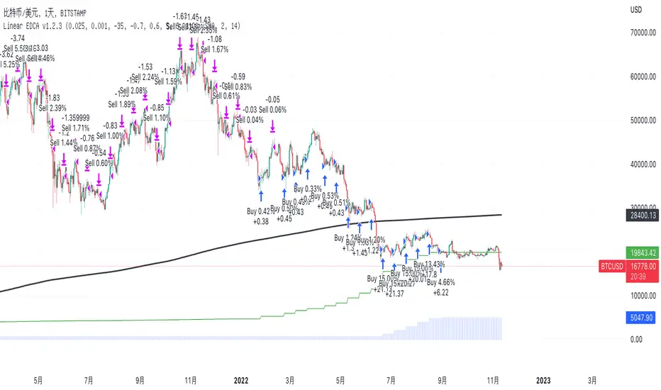
Reynolds warning rateIn fluid mechanics, the Reynolds number is the ratio of inertial forces to viscous forces within a fluid. Laminar flow occurs at low Reynolds numbers (i.e., viscous forces are dominant), whereas turbulent flow occurs at high Reynolds numbers (i.e., inertial forces are dominant). In the Turbulence indicator, I define that laminar flow occurs when simple moving averages have no interactions. In contrast, turbulent flow occurs when simple moving averages have chaotic interactions (i.e., irregular crossing and convergence).
Here, I calculate an economical analog of the Reynolds number developed by Jakimowicz and Juzwiszyn (2015). Furthermore, I propose the Reynolds Warning Rate, given by a ratio of short- and long-term Reynolds number.
The higher Reynolds Warning Rate indicates that price movement is going to a turbulence phase, and the market is under a possible systemic risk.
Reference:
Jakimowicz A, Juzwiszyn J (2015) Balance in the turbulent world of economy. Acta Physica Polonica A 127, 78–85.
Trading The Loonie (CADUSD)A port of the trading strategy described at technical.traders.com
"In “Trading The Loonie,” which appeared in the December 2015 issue of STOCKS & COMMODITIES, author Markos Katsanos
explains the heavy correlation between the Canadian dollar and crude oil. He then goes on to describe how one could
trade this correlation. Using similar logic as that employed in Bollinger Bands, Katsanos has built a study to
provide buy and sell signals for trading the Canadian dollar future."
See Also:
- Backtesting and forwardtesting (of TradingView Strategies)
- 9 Mistakes Quants Make that Cause Backtests to Lie (blog.quantopian.com)
- When Backtests Meet Reality (financial-hacker.com)
- Why MT4 backtesting does not work (www.stevehopwoodforex.com)