Reflex & Trendflex█ OVERVIEW
Reflex and Trendflex are zero-lag oscillators that decompose price into independent cycle and trend components using SuperSmoother filtering. These indicators isolate each component separately, providing clearer identification of cyclical reversals (Reflex) versus trending movements (Trendflex).
Based on Dr. John F. Ehlers' "Reflex: A New Zero-Lag Indicator" article (February 2020, TASC), both oscillators use normalized slope deviation analysis to minimize lag while maintaining signal clarity. The SuperSmoother filter removes high-frequency noise, then deviations from linear regression (Reflex) or current value (Trendflex) are measured and normalized by RMS for consistent amplitude across instruments and timeframes.
█ CONCEPTS
SuperSmoother Filter
Both oscillators begin with a two-pole Butterworth low-pass filter that smooths price data without the excessive lag of simple moving averages. The filter uses exponential decay coefficients and cosine modulation based on the cutoff period, providing aggressive smoothing while preserving signal timing.
Reflex: Cycle Component
Reflex isolates cyclical price behavior by measuring deviation from a linear regression line fitted through the SuperSmoother output. For each bar, the filter calculates a linear slope over the lookback period, then sums how much the smoothed price deviates from this trendline. These deviations represent pure cyclical movement - price oscillations around the dominant trend. The result is normalized by RMS (root mean square) to produce consistent amplitude regardless of volatility or timeframe.
Trendflex: Trend Component
Trendflex extracts trending behavior by measuring cumulative deviation from the current SuperSmoother value. Instead of comparing to a regression line, it simply sums the differences between the current smoothed value and all past values in the period. This captures sustained directional movement rather than oscillations. Like Reflex, normalization by RMS ensures comparable readings across different instruments.
RMS Normalization
Both oscillators normalize their raw deviation measurements using an exponentially weighted RMS calculation: `rms = 0.04 * deviation² + 0.96 * rms `. This adaptive normalization ensures the oscillator amplitude remains stable as volatility changes, making threshold levels meaningful across different market conditions.
█ INTERPRETATION
Reflex (Cycle Component)
Oscillates around zero representing cyclical price behavior isolated from trend:
• Above zero : Price is in upward phase of cycle
• Below zero : Price is in downward phase of cycle
• Zero crossings : Potential cycle reversal points
• Extremes : Indicate stretched cyclical condition, often precede mean reversion
Best used for identifying cyclical turning points in ranging or oscillating markets. More sensitive to reversals than Trendflex.
Trendflex (Trend Component)
Oscillates around zero representing trending behavior isolated from cycles:
• Above zero : Sustained upward trend
• Below zero : Sustained downward trend
• Zero crossings : Trend direction changes
• Magnitude : Strength of trend (larger absolute values = stronger trend)
Best used for confirming trend direction and identifying trend exhaustion. Less noisy than Reflex due to focus on directional movement rather than oscillations.
Combined Analysis
Using both oscillators together provides powerful signal confirmation:
• Both positive: Strong uptrend with positive cycle phase (high probability long setup)
• Both negative: Strong downtrend with negative cycle phase (high probability short setup)
• Divergent signals: Conflicting cycle and trend (choppy conditions, reduce position size)
• Reflex reversal with Trendflex agreement: Cyclical turn within established trend (entry/exit timing)
Dynamic Thresholds
Threshold bands identify statistically significant oscillator readings that warrant attention:
• Breach above +threshold : Strong bullish cycle (Reflex) or trend (Trendflex) behavior - potential overbought condition
• Breach below -threshold : Strong bearish cycle or trend behavior - potential oversold condition
• Return inside thresholds : Signal strength normalizing, potential reversal or consolidation ahead
• Threshold compression : During low volatility, thresholds narrow (especially with StdDev mode), making breaches more frequent
• Threshold expansion : During high volatility, thresholds widen, filtering out minor oscillations
Combine threshold breaches with zero-line position for stronger signals:
• Threshold breach + zero-line cross = high-conviction signal
• Threshold breach without zero-line support = monitor for confirmation
Alert Conditions
Six built-in alerts trigger on bar close (no repainting):
• Above +Threshold : Oscillator crossed above positive threshold (strong bullish behavior)
• Below -Threshold : Oscillator crossed below negative threshold (strong bearish behavior)
• Reflex Above Zero : Reflex crossed above zero (bullish cycle phase)
• Reflex Below Zero : Reflex crossed below zero (bearish cycle phase)
• Trendflex Above Zero : Trendflex crossed above zero (bullish trend shift)
• Trendflex Below Zero : Trendflex crossed below zero (bearish trend shift)
█ SETTINGS & PARAMETER TUNING
Oscillator Settings
• Source : Price series to decompose
• Reflex Period (5-50): SuperSmoother period for cycle component. Lower values increase responsiveness to cyclical turns but add noise. Default 20.
• Trendflex Period (5-50): SuperSmoother period for trend component. Lower values respond faster to trend changes. Default 20.
Display Settings
• Reflex/Trendflex Display : Toggle visibility and customize colors for each oscillator independently
• Zero Line : Reference line showing neutral oscillator position
Dynamic Thresholds
Optional significance bands that identify when oscillator readings indicate strong cyclical or trending behavior:
• Threshold Mode : Choose calculation method based on market characteristics
- MAD (Median Absolute Deviation) : Outlier-resistant, best for markets with occasional spikes (default)
- Standard Deviation : Volatility-sensitive, adapts quickly to regime changes
- Percentile Rank : Fixed probability bands (e.g., 90% = only 10% of values exceed threshold)
• Apply To : Select which oscillator (Reflex or Trendflex) to calculate thresholds for
• Period (2-200): Lookback window for threshold calculation. Default 50.
• Multiplier (k) : Scaling factor for MAD/StdDev modes. Higher values = fewer threshold breaches (default 1.5)
• Percentile (%) : For Percentile mode only. Higher percentile = more selective threshold (default 90%)
Parameter Interactions
• Shorter periods make both oscillators more sensitive but noisier
• Reflex typically more volatile than Trendflex at same period settings
• For ranging markets: shorter Reflex period (10-15) captures swings better
• For trending markets: shorter Trendflex period (10-15) follows trend shifts faster
█ LIMITATIONS
Inherent Characteristics
• Near-zero lag, not zero-lag : Despite the name, some lag remains from SuperSmoother filtering
• Normalization artifacts : RMS normalization can produce unusual readings during volatility regime changes
• Period dependency : Oscillator characteristics change significantly with different period settings - no "correct" universal parameter
Market Conditions to Avoid
• Very low volatility : Normalization amplifies noise in quiet markets, producing false signals
• Sudden gaps : SuperSmoother assumes continuous data; large gaps disrupt filter continuity requiring bars to stabilize
• Micro timeframes : Sub-minute charts contain microstructure noise that overwhelms signal quality
Parameter Selection Pitfalls
• Matching periods to dominant cycle : If period doesn't align with actual market cycle period, signals degrade
• Threshold over-tuning : Optimizing threshold parameters for past data often fails forward - use conservative defaults
• Ignoring component differences : Reflex and Trendflex measure different aspects - don't expect identical behavior
█ NOTES
Credits
These indicators are based on Dr. John F. Ehlers' "Reflex: A New Zero-Lag Indicator" published in the February 2020 issue of Technical Analysis of Stocks & Commodities (TASC) magazine. The article introduces a novel approach to isolating cycle and trend components using SuperSmoother filtering combined with normalized deviation analysis.
For those interested in the underlying mathematics and DSP concepts:
• Ehlers, J.F. (February 2020). "Reflex: A New Zero-Lag Indicator" - Technical Analysis of Stocks & Commodities magazine
• Ehlers, J.F. (2001). Rocket Science for Traders: Digital Signal Processing Applications . John Wiley & Sons
• Various TASC articles by John Ehlers on SuperSmoother filters and oscillator design
by ♚@e2e4
Cerca negli script per "gaps"

GAP DETECTORGAP DETECTOR is an indicator displaying price gaps that have never been completely filled (only gaps >= 5 pips are considered).
Each gap is defined by two lines (the lower and upper bound of the gap), and a label giving information on its price range
#Parameters:
length: the number of candles being considered in the indicator (max is 3000).
width: the width of the gap lines.

[PX] VWAP Gap LevelHello guys,
another day, another method for detecting support and resistance level. This time it's all about the VWAP and daily gaps it might produce.
How does it work?
The indicator detects when a new daily candle begins and the VWAP makes a big move in either direction. Often it produces a gap and this is where the support or resistance level will be plotted. The idea behind it is, that those gaps get filled at some point in time. You can control how big a VWAP movement ("gap") has to be with the "VWAP Movement %" -setting. Also, you can adjust the style of the level.
If you find this indicator useful, please leave a "like" and hit that "follow" button :)
Have fun and happy trading :)))

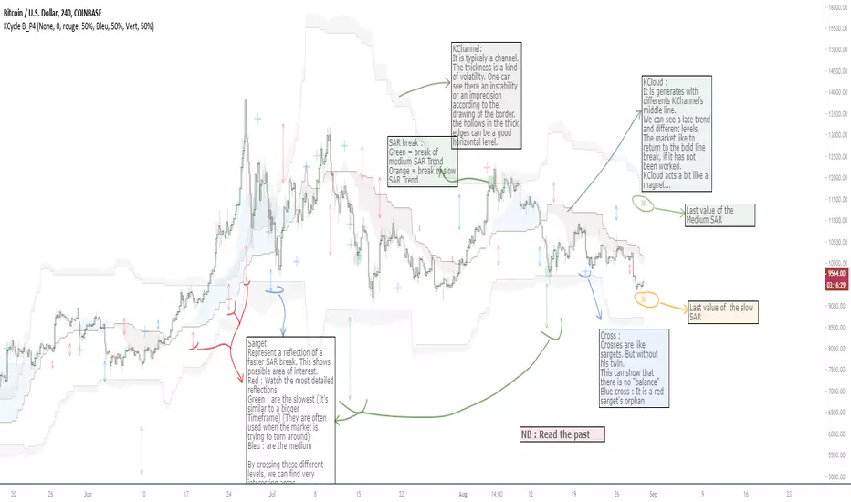
OVL_Kikoocycle Beta_Pine3This script use :
- A custom Chande Kroll Stop for generate the channel
- Some custom Parabolic S.A.R for generate cycles
This script can be separated into 3 categories:
- Channel Kroll generator : one layer for the actual interval and a layer for a Large Timeframe .(with ratio)
- "Range" generator : one layer for actual Interval and a layer for a Large Timeframe.(with automique ratio)
-Targets generator : one layer for actual interval with different trend.
"Channel Kroll" :
- I "hijack" the Chande Kroll Stop formula with custom parameters for generate this channel. Overall, it works like other types of channels like BB, etc... A midline and two borders. The thickness of the borders are relatively important here. A thick border shows some resistance of the area. And so the probability of seeing the market return to its first contact is stronger. While a very thin and vertical border would rather play the role of a breach, a bit like the idea of gaps. Often the market seems to want to go after several cycles.
You can activate its Large TimeFrame version, its midline is strong and fine borders helps to judge the risk.
SARget + "SAR Limited" :
- (S.A.R + targets) The philosophy of this function is simple... When a small cycle is broken, it creates a mark on a higher cycle. So on until the SAR called "SAR Limited". For simplicity, imagine a fractal image but inverted ... Break the small figure, it will mark the larger figure at this time but to get there you still have to make the way to the small figure.
Targets are : cross ("+") for fast targets(hidden by default because, theire work only on lower interval), squares (for medium trend), Xcross(for large trend) and red cross(they try to find a large contexte). When a target proc, it is for later (market need some cycles for going to, but it is relative to your interval). This gives you speculative goals.
Why 2 targets for a same type and a triangle with a 90deg angle : This give a potential area for management.The triangle help to visualize the SAR and to juge the market reaction. You need to adapte your trade with that...
Targets may be slightly too far because I am a bad coder... Currently the targets appear at the moment of rupture but it would be necessary to wait for the end of the breaking movement. Which can bring a positional error if the break is violent.
RnG and LTF RnG :
- Attempt to generate a Fibo range for each cycle and see interressing areas to enter or exit. This is played with the same philosophy as the Fibo extensions and retracement.
When a new RnG is generated, do not rush. It appears showing 50/50 for both sides. When a new RnG is generated, do not rush. It appears showing 50/50 for both sides. As long as the market is out of the middle zone (the 3 lines) keep in mind the past RnG.
When the market is out of range, you can use the FibRetracement tool for have extensions. One point at each end, as on the presentation graph. (Values 1.14, 1.272, 1.414, 1.618, 1.786, 2, 2.4 and 4 work well.) If too extrem you can active the LTF version.
Never fomo a break, market like to pull a level... Observe and be patient.
It's easier to use than to explain xD
NB : Do not use the LTF as context. For this, it is better to look at a higher interval.
I invite you to look in the style tab of the script and deselect the plots named UNCHECKEME, this will ease your browser.
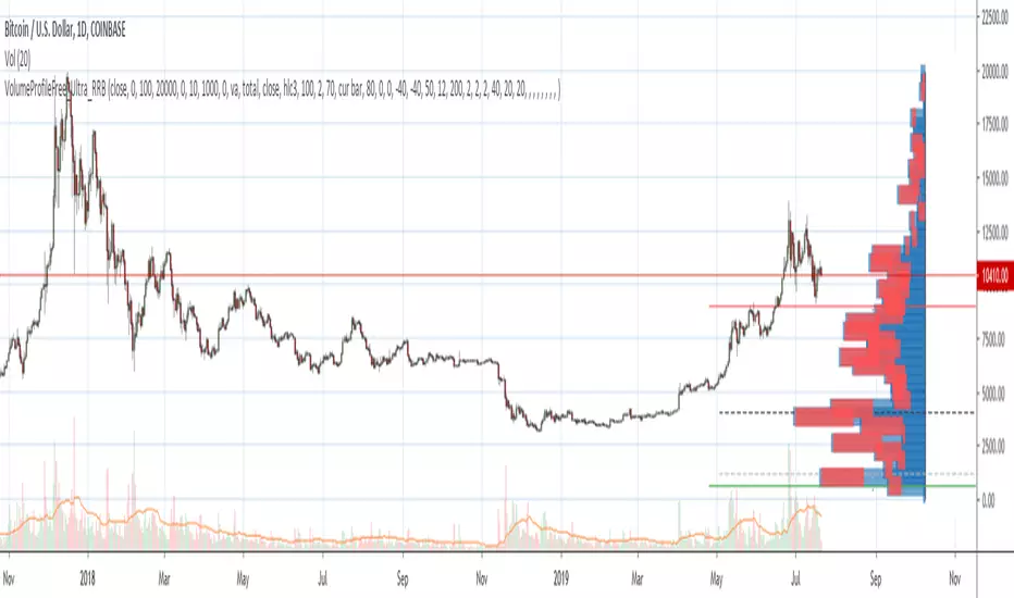
Volume Profile Free Ultra SLI (100 Levels Value Area VWAP) - RRBVolume Profile Free Ultra SLI by RagingRocketBull 2019
Version 1.0
This indicator calculates Volume Profile for a given range and shows it as a histogram consisting of 100 horizontal bars.
This is basically the MAX SLI version with +50 more Pinescript v4 line objects added as levels.
It can also show Point of Control (POC), Developing POC, Value Area/VWAP StdDev High/Low as dynamically moving levels.
Free accounts can't access Standard TradingView Volume Profile, hence this indicator.
There are several versions: Free Pro, Free MAX SLI, Free Ultra SLI, Free History. This is the Free Ultra SLI version. The Differences are listed below:
- Free Pro: 25 levels, +Developing POC, Value Area/VWAP High/Low Levels, Above/Below Area Dimming
- Free MAX SLI: 50 levels, 2x SLI modes for Buy/Sell or even higher res 150 levels
- Free Ultra SLI: 100 levels, packed to the limit, 2x SLI modes for Buy/Sell or even higher res 300 levels
- Free History: auto highest/lowest, historic poc/va levels for each session
Features:
- High-Res Volume Profile with up to 100 levels (line implementation)
- 2x SLI modes for even higher res: 300 levels with 3x vertical SLI, 100 buy/sell levels with 2x horiz SLI
- Calculate Volume Profile on full history
- POC, Developing POC Levels
- Buy/Sell/Total volume modes
- Side Cover
- Value Area, VAH/VAL dynamic levels
- VWAP High/Low dynamic levels with Source, Length, StdDev as params
- Show/Hide all levels
- Dim Non Value Area Zones
- Custom Range with Highlighting
- 3 Anchor points for Volume Profile
- Flip Levels Horizontally
- Adjustable width, offset and spacing of levels
- Custom Color for POC/VA/VWAP levels, Transparency for buy/sell levels
WARNING:
- Compilation Time: 1 min 20 sec
Usage:
- specify max_level/min_level/spacing (required)
- select range (start_bar, range length), confirm with range highlighting
- select volume type: Buy/Sell/Total
- select mode Value Area/VWAP to show corresponding levels
- flip/select anchor point to position the buy/sell levels
- use Horiz Buy/Sell SLI mode with 100 or Vertical SLI with 300 levels if needed
- use POC/Developing POC/VA/VWAP High/Low as S/R levels. Usually daily values from 1-3 days back are used as levels for the current day.
SLI:
use SLI modes to extend the functionality of the indicator:
- Horiz Buy/Sell 2x SLI lets you view 100 Buy/Sell Levels at the same time
- Vertical Max_Vol 3x SLI lets you increase the resolution to 300 levels
- you need at least 2 instances of the indicator attached to the same chart for SLI to work
1) Enable Horiz SLI:
- attach 2 indicator instances to the chart
- make sure all instances have the same min_level/max_level/range/spacing settings
- select volume type for each instance: you can have a buy/sell or buy/total or sell/total SLI. Make sure your buy volume instance is the last attached to be displayed on top of sell/total instances without overlapping.
- set buy_sell_sli_mode to true for indicator instances with volume_type = buy/sell, for type total this is optional.
- this basically tells the script to calculate % lengths based on total volume instead of individual buy/sell volumes and use ext offset for sell levels
- Sell Offset is calculated relative to Buy Offset to stack/extend sell after buy. Buy Offset = Zero - Buy Length. Sell Offset = Buy Offset - Sell Length = Zero - Buy Length - Sell Length
- there are no master/slave instances in this mode, all indicators are equal, poc/va levels are not affected and can work independently, i.e. one instance can show va levels, another - vwap.
2) Enable Vertical SLI:
- attach the first instance and evaluate the full range to roughly determine where is the highest max_vol/poc level i.e. 0..20000, poc is in the bottom half (third, middle etc) or
- add more instances and split the full vertical range between them, i.e. set min_level/max_level of each corresponding instance to 0..10000, 10000..20000 etc
- make sure all instances have the same range/spacing settings
- an instance with a subrange containing the poc level of the full range is now your master instance (bottom half). All other instances are slaves, their levels will be calculated based on the max_vol/poc of the master instance instead of local values
- set show_max_vol_sli to true for the master instance. for slave instances this is optional and can be used to check if master/slave max_vol values match and slave can read the master's value. This simply plots the max_vol value
- you can also attach all instances and set show_max_vol_sli to true in all of them - the instance with the largest max_vol should become the master
Auto/Manual Ext Max_Vol Modes:
- for auto vertical max_vol SLI mode set max_vol_sli_src in all slave instances to the max_vol of the master indicator: "VolumeProfileFree_MAX_RRB: Max Volume for Vertical SLI Mode". It can be tricky with 2+ instances
- in case auto SLI mode doesn't work - assign max_vol_sli_ext in all slave instances the max_vol value of the master indicator manually and repeat on each change
- manual override max_vol_sli_ext has higher priority than auto max_vol_sli_src when both values are assigned, when they are 0 and close respectively - SLI is disabled
- master/slave max_vol values must match on each bar at all times to maintain proper level scale, otherwise slave's levels will look larger than they should relative to the master's levels.
- Max_vol (red) is the last param in the long list of indicator outputs
- the only true max_vol/poc in this SLI mode is the master's max_vol/poc. All poc/va levels in slaves will be irrelevant and are disabled automatically. Slaves can only show VWAP levels.
- VA Levels of the master instance in this SLI mode are calculated based on the subrange, not the whole range and may be inaccurate. Cross check with the full range.
WARNING!
- auto mode max_vol_sli_src is experimental and may not work as expected
- you can only assign auto mode max_vol_sli_src = max_vol once due to some bug with unhandled exception/buffer overflow in Tradingview. Seems that you can clear the value only by removing the indicator instance
- sometimes you may see a "study in error state" error when attempting to set it back to close. Remove indicator/Reload chart and start from scratch
- volume profile may not finish to redraw and freeze in an ugly shape after an UI parameter change when max_vol_sli_src is assigned a max_vol value. Assign it to close - VP should redraw properly, but it may not clear the assigned max_vol value
- you can't seem to be able to assign a proper auto max_vol value to the 3rd slave instance
- 2x Vertical SLI works and tested in both auto/manual, 3x SLI - only manual seems to work (you can have a mixed mode: 2nd instance - auto, 3rd - manual)
Notes:
- This code uses Pinescript v3 compatibility framework
- This code is 20x-30x faster (main for cycle is removed) especially on lower tfs with long history - only 4-5 sec load/redraw time vs 30-60 sec of the old Pro versions
- Instead of repeatedly calculating the total sum of volumes for the whole range on each bar, vol sums are now increased on each bar and passed to the next in the range making it a per range vs per bar calculation that reduces time dramatically
- 100 levels consist of 50 main plot levels and 50 line objects used as alternate levels, differences are:
- line objects are always shown on top of other objects, such as plot levels, zero line and side cover, it's not possible to cover/move them below.
- all line objects have variable lengths, use actual x,y coords and don't need side cover, while all plot levels have a fixed length of 100 bars, use offset and require cover.
- all key properties of line objects, such as x,y coords, color can be modified, objects can be moved/deleted, while this is not possible for static plot levels.
- large width values cause line objects to expand only up/down from center while their length remains the same and stays within the level's start/end points similar to an area style.
- large width values make plot levels expand in all directions (both h/v), beyond level start/end points, sometimes overlapping zero line, making them an inaccurate % length representation, as opposed to line objects/plot levels with area style.
- large width values translate into different widths on screen for line objects and plot levels.
- you can't compensate for this unwanted horiz width expansion of plot levels because width uses its own units, that don't translate into bars/pixels.
- line objects are visible only when num_levels > 50, plot levels are used otherwise
- Since line objects are lines, plot levels also use style line because other style implementations will break the symmetry/spacing between levels.
- if you don't see a volume profile check range settings: min_level/max_level and spacing, set spacing to 0 (or adjust accordingly based on the symbol's precision, i.e. 0.00001)
- you can view either of Buy/Sell/Total volumes, but you can't display Buy/Sell levels at the same time using a single instance (this would 2x reduce the number of levels). Use 2 indicator instances in horiz buy/sell sli mode for that.
- Volume Profile/Value Area are calculated for a given range and updated on each bar. Each level has a fixed length. Offsets control visible level parts. Side Cover hides the invisible parts.
- Custom Color for POC/VA/VWAP levels - UI Style color/transparency can only change shape's color and doesn't affect textcolor, hence this additional option
- Custom Width - UI Style supports only width <= 4, hence this additional option
- POC is visible in both modes. In VWAP mode Developing POC becomes VWAP, VA High and Low => VWAP High and Low correspondingly to minimize the number of plot outputs
- You can't change buy/sell level colors from input (only transparency) - this requires 2x plot outputs => 2x reduces the number of levels to fit the max 64 limit. That's why 2 additional plots are used to dim the non Value Area zones
- You can change level transparency of line objects. Due to Pinescript limitations, only discrete values are supported.
- Inverse transp correlation creates the necessary illusion of "covered" line objects, although they are shown on top of the cover all the time
- If custom lines_transp is set the illusion will break because transp range can't be skewed easily (i.e. transp 0..100 is always mapped to 100..0 and can't be mapped to 50..0)
- transparency can applied to lines dynamically but nva top zone can't be completely removed because plot/mixed type of levels are still used when num_levels < 50 and require cover
- transparency can't be applied to plot levels dynamically from script this can be done only once from UI, and you can't change plot color for the past length bars
- All buy/sell volume lengths are calculated as % of a fixed base width = 100 bars (100%). You can't set show_last from input to change it
- Range selection/Anchoring is not accurate on charts with time gaps since you can only anchor from a point in the future and measure distance in time periods, not actual bars, and there's no way of knowing the number of future gaps in advance.
- Adjust Width for Log Scale mode now also works on high precision charts with small prices (i.e. 0.00001)
- in Adjust Width for Log Scale mode Level1 width extremes can be capped using max deviation (when level1 = 0, shift = 0 width becomes infinite)
- There's no such thing as buy/sell volume, there's just volume, but for the purposes of the Volume Profile method, assume: bull candle = buy volume, bear candle = sell volume
P.S. I am your grandfather, Luke! Now, join the Dark Side in your father's steps or be destroyed! Once more the Sith will rule the Galaxy, and we shall have peace...
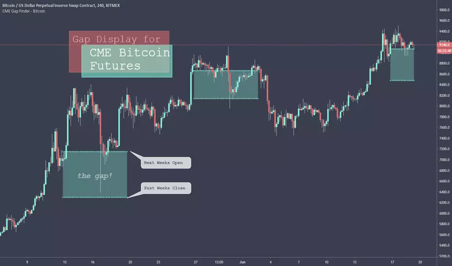
CME Gap Finder - BitcoinOnly for Bitcoin!
This indicator locates weekly gaps created by the CME Futures market for Bitcoin.
As you can see, Bitcoin tends to close the weekly gaps created in the futures market so I thought this could be a very useful tool.
Instead of having to look between multiple charts, this simply overlays the past weeks open and close should a gap appear.
I hope you find this indicator useful!
Cheers!

Anchor ZonesL.A. Little, who wrote two books on trend trading, explained a key timing concept called anchor zones which was used, within his trading system, to enter and exit the market at appropriate times.
Anchor zones are formed from anchor bars. An anchor bar is a bar that has one or more of these components: wide range, high volume or gaps. For this script we're going to require two or more of the components. When an anchor bar forms, we'll note the high and low of the bar and draw a zone across time as prices develops. For this script, we'll also note the open and close of the candle to hint at other levels of support or resistance. The boundaries of these zones can act as support or resistance, but they also mark out the areas where price can often get trapped.
A breakout from these zones on high volume can suggest the beginning of a new trend. In general, anchor zones are a good compliment to price action strategies. For more information on how to use these, refer to L.A. Little's books.
References
onlinelibrary.wiley.com
www.tradingsetupsreview.com
Want to Learn?
If you'd like the opportunity to learn Pine but you have difficulty finding resources to guide you, take a look at this rudimentary list: docs.google.com
The list will be updated in the future as more people share the resources that have helped, or continue to help, them. Follow me on Twitter to keep up-to-date with the growing list of resources.
Suggestions or Questions?
Don't even kinda hesitate to forward them to me. My (metaphorical) door is always open.

T2-%Use a superposition of 30 avarages to stress-out trend changes (points in time where all possible frequencies that create the movment change their phase from prositive to negetive or the opposite). The indicator has one paramater that should be adjusted: 'os'.
By defult the 30 avarages that are tested range from 7 to 63 in gaps of 2. increasing the 'os' parameter moves the ranges by multiplications of 65. therefore if you add 5 indicators ontop of eachother, each scaled to left and set the os of each to another value (0,1,2,3,4) you will have a full spectum of avarages ranging from 7 to 325 in gaps of 2.
GapologyThis indicator can be used as a simple measure of price action tradability. It's an alternative to volume that focuses on the gaps between close and open candle prices. The bigger the gaps, the more spread and slippage you'll get when trading.

Hersheys Volume Pressure v2Hersheys Volume Pressure gives you very nice confirmation of trend starts and stops using volume and price.
For up bars...
If you have a large price change with low volume , that's very bullish .
If you have a small price change with low volume , that's bullish .
For down bars...
If you have a large price change with low volume , that's very bearish .
If you have a small price change with low volume , that's bearish .
Look at the chart and you'll see how trends start and end with a PINCH and widen in the middle of the moves.
You can set the moving average period, 14 is the default.
Good trading!
Brian Hershey
v2 change log...
- issue with price gaps - gaps at the open were sometimes showing incorrect colors
- scaling issues - sometimes a change is so large it scales down all nearby data and renders it hard to view. Code was added to clip those huge values.
v3 what's coming next...
- better scaling - sometimes with thinly traded stocks there is too much clipping. For now increase the chart interval to correct.


eBacktesting - Learning: FVGeBacktesting - Learning: FVG is an indicator in the eBacktesting Learning series: a collection of tools designed to help new traders understand the most important concepts in trading through clear, visual examples directly on the chart.
This indicator highlights Fair Value Gaps (FVGs): areas where price moved so quickly that it left behind an imbalance. These zones often act like "magnets" for future price action and can become important areas to watch for reactions, continuations, or reversals.
To keep the chart clean and the learning process practical, FVGs are only displayed when they remain relevant, meaning they are not instantly cleared by the very next candle. This helps beginners focus on the imbalances that actually persist and are more likely to matter.
Each FVG is drawn as a zone with a midpoint line and will visually update as price interacts with it:
Touched when price trades into the zone
Filled when price completely clears the zone
These indicators are built to pair perfectly with eBacktesting extension, where traders can practice these concepts step-by-step. Backtesting concepts visually like this is one of the fastest ways to learn, build confidence, and improve trading performance.
Educational use only. Not financial advice.

Ultimate Futures Daytrade Suite v1 - The Strategy GuideHere is the complete **Strategy Guide** translated into English.
---
# 📘 Ultimate Futures Daytrade Suite – The Strategy Guide
### 1. The Visual Legend (What is what?)
Before you trade, you need to understand the hierarchy of your lines. Not every line has the same importance.
* **🟣 Daily EMA 50 (Neon Violet):** The **"Big Boss"**. It determines the **Macro Trend**.
* *Price above:* We are primarily looking for Longs.
* *Price below:* We are primarily looking for Shorts.
* **🟢 4h EMA 50 (Neon Green):** The **"Swing Trend"**. Your most important level for **Pullback Entries** (Re-entries).
* **🟡 POC (Gold) & TPO:** The **"Magnet"**. Price often returns here.
* *Rule:* Never open a trade directly *on* the POC (Risk of "Chop"). Use it as a **Target** (Take Profit).
* **🟠 IB High/Low (Orange Lines):** The **"Daily Structure"**.
* A breakout from the IB (Initial Balance) often indicates the trend direction for the day.
* **🟥/🟩 Boxes (Supply/Demand):** Resistance and Support zones from the 1h timeframe.
* **⬜ FVG Boxes:** "Gaps" in the market that are often filled.
---
### 2. The Trading Workflow (Top-Down Method)
Go through this mental checklist before every trade:
#### Step 1: Trend Check (The Traffic Light)
Look at the **Violet Line (Daily)** and the **Green Line (4h)**.
* **Bullish:** Price is above Violet AND above Green. -> *Focus: Buy dips.*
* **Bearish:** Price is below Violet AND below Green. -> *Focus: Sell rallies.*
* **Mixed:** Price is between Violet and Green. -> *Caution! Market is undecided (Range Trading).*
#### Step 2: Location (The Context)
Where is the price currently located?
* Are we at a **Green Demand Zone**?
* Are we testing the **4h EMA 50 (Green)** from above?
* Are we at the **VWAP**?
* *Never trade in "No Man's Land"!* Wait until the price touches one of your lines.
#### Step 3: Trigger (The Execution)
Now zoom into your lower timeframe (e.g., 5min or 15min).
* Wait for a reaction at the zone.
* Use the **EMA 9 (Yellow)** as a momentum trigger. If price breaks the EMA 9 and closes above/below it, that is your "Go".
---
### 3. The Setup Blueprints
Here are the two most profitable scenarios you can trade with this script:
#### A) The "Golden Trend" Setup (Long)
* **Context:** Price > **Daily EMA (Violet)**.
* **Preparation:** Price corrects (drops) back to the **4h EMA 50 (Green)** or to the **VWAP**.
* **Confluence:** Ideally, there is also a **Demand Zone (Green Box)** or an **FVG** at that level.
* **Entry:** As soon as a candle touches the zone and closes bullish again (or reclaims the EMA 9).
* **Stop-Loss:** Below the 4h EMA 50.
* **Take-Profit:** Next **Supply Zone (Red)** or the **IB High (Orange)**.
#### B) The "Daytrade Breakout" (Intraday)
* **Context:** Price opens inside yesterday's Value Area.
* **Signal:** Price breaks through the **IB High (Orange)** with momentum.
* **Filter:** Price must be above the **VWAP**.
* **Entry:** On the retest of the IB High or directly on the breakout.
* **Target:** Price often trends in that direction for the rest of the day.
---
### 4. Warning Signals (When NOT to trade)
1. **The "Concrete Ceiling":** If you want to go Long, but the **Violet Daily EMA 50** is running directly above you. This is massive resistance. Better wait until it is broken.
2. **The "POC Dance":** If price is dancing sideways around the **Gold Line (POC)**. This is a "No-Trade Zone". Day traders lose the most money here due to fees and whipsaws.
3. **Overextension:** If price is extremely far away from the **4h EMA 50 (Green)** (Rubber Band Effect). Do not enter in the trend direction here; wait for a pullback to the line.
### Summary
Your chart is now telling you a story:
* **Violet** tells you the Direction.
* **Green** gives you the Entry.
* **Red/Green Boxes** show you the Obstacles.
* **Yellow (EMA 9)** gives you the Timing.
Good luck with the Suite! This is a setup similar to what institutional traders use.

Macro Risk Sentiment - Intermarket Timing SignalOverview
This indicator builds a composite macro sentiment score by analyzing intermarket relationships between bonds, credit spreads, the US dollar, and volatility. The core premise is that these markets often signal shifts in risk appetite before equities react, providing a timing edge for managing exposure.
When macro conditions favor risk assets, the indicator signals RISK-ON (green). When conditions deteriorate, it signals RISK-OFF (red). This is not a predictive tool but rather a systematic way to assess the current macro environment.
The Problem It Solves
Markets do not move in isolation. Before major equity drawdowns, stress often appears first in credit markets, bonds, and volatility. By monitoring these leading indicators systematically, we can identify periods when holding equity exposure carries elevated risk.
The goal is not to catch every move but to avoid the worst drawdowns by stepping aside when multiple macro factors align negatively.
How It Works
Step 1: Data Collection
The indicator pulls daily data from four key markets:
Risk-On Inputs (positive for equities when rising):
- TLT (20+ Year Treasury Bonds): Rising bonds can signal improving liquidity or flight-to-safety ending
- JNK (High-Yield Corporate Bonds): Rising junk bonds indicate credit conditions improving and risk appetite increasing
Risk-Off Inputs (negative for equities when rising):
- DXY (US Dollar Index): Strong dollar tightens global financial conditions and signals risk-off flows
- VIX (Volatility Index): Elevated VIX indicates fear and hedging demand
Step 2: Z-Score Normalization
Each input trades at different absolute levels, so direct comparison is impossible. The indicator converts each to a z-score: how many standard deviations the current value is from its 252-day (1 year) average.
A z-score of +1 means "unusually high relative to recent history." A z-score of -1 means "unusually low." This puts all inputs on the same scale.
Step 3: Composite Calculation
The macro score combines the normalized inputs:
Macro Score = (TLT z-score + JNK z-score) - (DXY z-score + VIX z-score)
The result is clamped between -1.5 and +1.5 to prevent outliers from dominating, then smoothed with an EMA to reduce noise.
Step 4: Signal Generation
Seven different methods are available for determining when conditions shift:
1. EMA Cross: Classic crossover between smoothed macro and its signal line
2. Slope: Simple direction of the macro trend
3. Momentum: Rate of change exceeding a threshold
4. Session Delta: Comparing today's reading to yesterday's
5. Pivot: Market structure analysis (higher lows vs lower highs)
6. Acceleration: Second derivative (is momentum increasing?)
7. Multi-Confirm: Requires 4 or more methods to agree
Why These Specific Markets?
Bonds (TLT)
Treasury bonds often lead equities at turning points. When institutions rotate into bonds, it signals caution. When they rotate out, it signals risk appetite returning.
Credit (JNK)
High-yield bonds price credit risk faster than equities. Widening credit spreads (falling JNK) often precede equity weakness by days or weeks.
Dollar (DXY)
A strong dollar creates headwinds for multinational earnings, tightens global USD liquidity, and signals defensive positioning globally.
Volatility (VIX)
The options market prices fear before it manifests in price. Sustained elevated VIX readings indicate hedging demand and uncertainty.
Research Application: Weekly Put Selling
One application of this indicator is timing premium-selling strategies. I tested using the EMA Cross method to filter 7-day-to-expiration (7DTE) put sales on ES futures with 90% Profit Target and 600% Stop Loss, only selling puts when the indicator showed RISK-ON.
Results with Macro Filter (2020-2025):
- Trades: 200
- Win Rate: 96.0%
- Total P/L: +$33,636
- Max Drawdown: 2.91%
- Profit Factor: 3.51
Results without Filter (same period):
- Trades: 357
- Win Rate: 96.1%
- Total P/L: +$63,492
- Max Drawdown: 10.30%
- Profit Factor: 2.90
Key Insight:
The filtered approach made less total profit (fewer trades) but reduced maximum drawdown by 72% (from 10.30% to 2.91%). This significantly improves risk-adjusted returns and allows for potentially higher position sizing with confidence.
Note: These results are from external backtesting on actual options data, not the TradingView backtest engine. Past performance does not guarantee future results.
Features
Seven configurable signal methods for different trading styles
Adjustable weights for each data source
Z-score normalization puts all inputs on equal footing
Visual info table showing all metrics at a glance
Background coloring for quick regime identification
Alert conditions for signal changes
Secondary plot showing method-specific metrics
Settings Guide
Macro Settings
Z-Score Lookback (default 252): Period for calculating standard deviations. 252 equals approximately one trading year. Longer periods are more stable but slower to adapt.
Macro EMA (default 7): Smoothing for the raw composite score. Lower values give faster but noisier signals.
Signal EMA (default 8): Secondary smoothing for the signal line. Used primarily in EMA Cross method.
Signal Method
EMA Cross : Recommended starting point. Signals when smoothed macro crosses its signal line.
Slope : Simpler approach based purely on trend direction.
Momentum : Requires rate of change to exceed a threshold.
Session Delta : Compares today to yesterday (daily timeframe focus).
Pivot : Uses market structure (higher lows for bullish, lower highs for bearish).
Acceleration : Measures change in slope (second derivative).
Multi-Confirm : Conservative approach requiring 4+ methods to agree.
Data Sources
Each source can be enabled/disabled and weighted from 0 to 3
Default is equal weighting (1.0) for all four sources
Experiment with emphasizing sources most relevant to your trading (tested on SPX)
How to Use
Basic Interpretation:
Green background / RISK-ON: Macro conditions favor equity exposure
Red background / RISK-OFF: Macro conditions suggest caution
Arrow markers indicate regime changes
For Risk Management:
Use RISK-OFF signals to reduce position size or hedge
Use RISK-ON signals to resume normal exposure
Consider the indicator as one input among many, not a complete system
For Options Strategies:
Avoid selling premium during RISK-OFF periods
Resume premium selling when RISK-ON returns
This approach trades frequency for reduced tail risk
Alert Setup:
Set alerts on "Bullish Turn" and "Bearish Turn" conditions
Receive notifications when the macro regime changes
Research Ideas
This indicator is designed as a research framework. Consider testing:
Different signal methods for your specific strategy
Adding or removing data sources based on what you trade
Varying the z-score lookback for different market regimes
Combining with price-based filters (moving averages, support/resistance)
Using the multi-confirm method for higher-conviction signals only
Limitations
The indicator uses daily data, so intraday signals may lag
Overnight gaps from surprise news cannot be anticipated
False signals will occur, especially in choppy, range-bound markets
The z-score lookback creates a recency bias; what was "normal" a year ago may not be relevant today
Not all drawdowns are preceded by macro deterioration; some come from idiosyncratic events
Past intermarket relationships may not persist in the future
Disclaimer
This indicator is for educational and research purposes only. It does not constitute financial advice.
Past performance does not guarantee future results
The research results shared are from historical backtesting and may not reflect actual trading conditions
Always conduct your own research and due diligence
Consider your personal risk tolerance before making any trading decisions
Never risk more than you can afford to lose
Credits
Intermarket analysis concepts draw from established macro trading principles. The multi-signal approach is original work designed to give users flexibility in how they interpret the macro data.

Fair Value Gaps (40+ Points) with NY Session AlertsFVG with alerts. This works for the NY session only.

[Greeny] RTH Only Naked VPOCWhat it does
Calculates and displays daily Volume Point of Control (VPOC) levels based on RTH (Regular Trading Hours) session only. Tracks which VPOCs remain "naked" (untouched) and which have been hit - but only counts hits during RTH hours, ignoring overnight/globex touches.
Key Features
One VPOC per trading day calculated from entire RTH session volume profile
RTH-only hit detection - levels only marked as hit when touched during RTH, not overnight
Works on all timeframes - daily, hourly, or any chart timeframe
Volume-based filtering - automatically skips low-liquidity sessions (pre-front-month contract data)
Visual markers - small dash on origin bar shows where each VPOC was, even after being hit
Visual Guide
Yellow dashed line - Naked VPOC (not yet touched during RTH)
White dashed line - Hit VPOC (was touched during RTH)
Small dash on candle - POC origin marker
Settings
Display options: Toggle to show only naked POCs, customize hit/naked colors, adjust line width and style (solid/dashed/dotted), enable/disable line extension and origin markers.
RTH Session: Configure start and end time in NY timezone. Default is 9:30-16:00 (US equity market hours), which equals 15:30-22:00 Budapest time.
Advanced: Adjust volume profile resolution (default 250 bins), data source timeframe for calculations (5min recommended for daily charts), and minimum volume threshold to filter out low-liquidity sessions like pre-rollover contract data (default 10% of average).
Best For
ES/MES, NQ/MNQ futures traders
Mean reversion strategies using VPOC as support/resistance
Auction Market Theory practitioners
Anyone wanting clean RTH-only volume profile levels
Note on Contract Rollovers
When using specific contract symbols (e.g., ESH2026 instead of ES1!), the script may show many naked VPOCs from months before the contract became active. This happens because futures contracts have very low liquidity before becoming the front-month, creating unreliable VPOCs with gaps that never get hit. The volume filter helps reduce this, but you may need to increase the "Min Volume % of Average" setting or simply ignore older levels when viewing back-month data.

Smart Money Flow Oscillator [MarkitTick]💡This script introduces a sophisticated method for analyzing market liquidity and institutional order flow. Unlike traditional volume indicators that treat all market activity equally, the Smart Money Flow Oscillator (SMFO) employs a Logic Flow Architecture (LFA) to filter out market noise and "churn," focusing exclusively on high-impact, high-efficiency price movements. By synthesizing price action, volume, and relative efficiency, this tool aims to visualize the accumulation and distribution activities that are often attributed to "smart money" participants.
✨ Originality and Utility
Standard indicators like On-Balance Volume (OBV) or Money Flow Index (MFI) often suffer from noise because they aggregate volume based simply on the close price relative to the previous close, regardless of the quality of the move. This script differentiates itself by introducing an "Efficiency Multiplier" and a "Momentum Threshold." It only registers volume flow when a price move is considered statistically significant and structurally efficient. This creates a cleaner signal that highlights genuine supply and demand imbalances while ignoring indecisive trading ranges. It combines the trend-following nature of cumulative delta with the mean-reverting insights of an In/Out ratio, offering a dual-mode perspective on market dynamics.
🔬 Methodology
The underlying calculation of the SMFO relies on several distinct quantitative layers:
• Efficiency Analysis
The script calculates a "Relative Efficiency" ratio for every candle. This compares the current price displacement (body size) per unit of volume against the historical average.
If price moves significantly with relatively low volume, or proportional volume, it is deemed "efficient."
If significant volume occurs with little price movement (churn/absorption), the efficiency score drops.
This score is clamped between a user-defined minimum and maximum (Efficiency Cap) to prevent outliers from distorting the data.
• Momentum Thresholding
Before adding any data to the flow, the script checks if the current price change exceeds a volatility threshold derived from the previous candle's open-close range. This acts as a gatekeeper, ensuring that only "strong" moves contribute to the oscillator.
• Variable Flow Calculation
If a move passes the threshold, the script calculates the flow value by multiplying the Typical Price and Volume (Money Flow) by the calculated Efficiency Multiplier.
Bullish Flow: Strong upward movement adds to the positive delta.
Bearish Flow: Strong downward movement adds to the negative delta.
Neutral: Bars that fail the momentum threshold contribute zero flow, effectively flattening the line during consolidation.
• Calculation Modes
Cumulative Delta Flow (CDF): Sums the flow values over a rolling period. This creates a trend-following oscillator similar to OBV but smoother and more responsive to real momentum.
In/Out Ratio: Calculates the percentage of bullish inflow relative to the total absolute flow over the period. This oscillates between 0 and 100, useful for identifying overextended conditions.
📖 How to Use
Traders can utilize this oscillator to identify trend strength and potential reversals through the following signals:
• Signal Line Crossovers
The indicator plots the main Flow line (colored gradient) and a Signal line (grey).
Bullish (Green Cloud): When the Flow line crosses above the Signal line, it suggests rising buying pressure and efficient upward movement.
Bearish (Red Cloud): When the Flow line crosses below the Signal line, it suggests dominating selling pressure.
• Divergences
The script automatically detects and plots divergences between price and the oscillator:
Regular Divergence (Solid Lines): Suggests a potential trend reversal (e.g., Price makes a Lower Low while Oscillator makes a Higher Low).
Hidden Divergence (Dashed Lines): Suggests a potential trend continuation (e.g., Price makes a Higher Low while Oscillator makes a Lower Low).
"R" labels denote Regular, and "H" labels denote Hidden divergences.
• Dashboard
A dashboard table is displayed on the chart, providing real-time metrics including the current Efficiency Multiplier, Net Flow value, and the active mode status.
• In/Out Ratio Levels
When using the Ratio mode:
Values above 50 indicate net buying pressure.
Values below 50 indicate net selling pressure.
Approaching 70 or 30 can indicate overbought or oversold conditions involving volume exhaustion.
⚙️ Inputs and Settings
Calculation Mode: Choose between "Cumulative Delta Flow" (Trend focus) or "In/Out Ratio" (Oscillator focus).
Auto-Adjust Period: If enabled, automatically sets the lookback period based on the chart timeframe (e.g., 21 for Daily, 52 for Weekly).
Manual Period: The rolling lookback length for calculations if Auto-Adjust is disabled.
Efficiency Length: The period used to calculate the average body and volume for the efficiency baseline.
Eff. Min/Max Cap: Limits the impact of the efficiency multiplier to prevent extreme skewing during anomaly candles.
Momentum Threshold: A factor determining how much price must move relative to the previous candle to be considered a "strong" move.
Show Dashboard/Divergences: Toggles for visual elements.
🔍 Deconstruction of the Underlying Scientific and Academic Framework
This indicator represents a hybrid synthesis of academic Market Microstructure theory and classical technical analysis. It utilizes an advanced algorithm to quantify "Price Impact," leveraging the following theoretical frameworks:
• 1. The Amihud Illiquidity Ratio (2002)
The core logic (calculating body / volume) functions as a dynamic implementation of Yakov Amihud’s Illiquidity Ratio. It measures price displacement per unit of volume. A high efficiency score indicates that "Smart Money" has moved the price significantly with minimal resistance, effectively highlighting liquidity gaps or institutional control.
• 2. Kyle’s Lambda (1985) & Market Depth
Drawing from Albert Kyle’s research on market microstructure, the indicator approximates Kyle's Lambda to measure the elasticity of price in response to order flow. By analyzing the "efficiency" of a move, it identifies asymmetries—specifically where price reacts disproportionately to low volume—signaling potential manipulation or specific Market Maker activity.
• 3. Wyckoff’s Law of Effort vs. Result
From a classical perspective, the algorithm codifies Richard Wyckoff’s "Effort vs. Result" logic. It acts as an oscillator that detects anomalies where "Effort" (Volume) diverges from the "Result" (Price Range), predicting potential reversals.
• 4. Quantitative Advantage: Efficiency-Weighted Volume
Unlike linear indicators such as OBV or Chaikin Money Flow—which treat all volume equally—this indicator (LFA) utilizes Efficiency-Weighted Volume. By applying the efficiency_mult factor, the algorithm filters out market noise and assigns higher weight to volume that drives structural price changes, adopting a modern quantitative approach to flow analysis.
● Disclaimer
All provided scripts and indicators are strictly for educational exploration and must not be interpreted as financial advice or a recommendation to execute trades. I expressly disclaim all liability for any financial losses or damages that may result, directly or indirectly, from the reliance on or application of these tools. Market participation carries inherent risk where past performance never guarantees future returns, leaving all investment decisions and due diligence solely at your own discretion.

Adaptive Market Wave TheoryAdaptive Market Wave Theory
🌊 CORE INNOVATION: PROBABILISTIC PHASE DETECTION WITH MULTI-AGENT CONSENSUS
Adaptive Market Wave Theory (AMWT) represents a fundamental paradigm shift in how traders approach market phase identification. Rather than counting waves subjectively or drawing static breakout levels, AMWT treats the market as a hidden state machine —using Hidden Markov Models, multi-agent consensus systems, and reinforcement learning algorithms to quantify what traditional methods leave to interpretation.
The Wave Analysis Problem:
Traditional wave counting methodologies (Elliott Wave, harmonic patterns, ABC corrections) share fatal weaknesses that AMWT directly addresses:
1. Non-Falsifiability : Invalid wave counts can always be "recounted" or "adjusted." If your Wave 3 fails, it becomes "Wave 3 of a larger degree" or "actually Wave C." There's no objective failure condition.
2. Observer Bias : Two expert wave analysts examining the same chart routinely reach different conclusions. This isn't a feature—it's a fundamental methodology flaw.
3. No Confidence Measure : Traditional analysis says "This IS Wave 3." But with what probability? 51%? 95%? The binary nature prevents proper position sizing and risk management.
4. Static Rules : Fixed Fibonacci ratios and wave guidelines cannot adapt to changing market regimes. What worked in 2019 may fail in 2024.
5. No Accountability : Wave methodologies rarely track their own performance. There's no feedback loop to improve.
The AMWT Solution:
AMWT addresses each limitation through rigorous mathematical frameworks borrowed from speech recognition, machine learning, and reinforcement learning:
• Non-Falsifiability → Hard Invalidation : Wave hypotheses die permanently when price violates calculated invalidation levels. No recounting allowed.
• Observer Bias → Multi-Agent Consensus : Three independent analytical agents must agree. Single-methodology bias is eliminated.
• No Confidence → Probabilistic States : Every market state has a calculated probability from Hidden Markov Model inference. "72% probability of impulse state" replaces "This is Wave 3."
• Static Rules → Adaptive Learning : Thompson Sampling multi-armed bandits learn which agents perform best in current conditions. The system adapts in real-time.
• No Accountability → Performance Tracking : Comprehensive statistics track every signal's outcome. The system knows its own performance.
The Core Insight:
"Traditional wave analysis asks 'What count is this?' AMWT asks 'What is the probability we are in an impulsive state, with what confidence, confirmed by how many independent methodologies, and anchored to what liquidity event?'"
🔬 THEORETICAL FOUNDATION: HIDDEN MARKOV MODELS
Why Hidden Markov Models?
Markets exist in hidden states that we cannot directly observe—only their effects on price are visible. When the market is in an "impulse up" state, we see rising prices, expanding volume, and trending indicators. But we don't observe the state itself—we infer it from observables.
This is precisely the problem Hidden Markov Models (HMMs) solve. Originally developed for speech recognition (inferring words from sound waves), HMMs excel at estimating hidden states from noisy observations.
HMM Components:
1. Hidden States (S) : The unobservable market conditions
2. Observations (O) : What we can measure (price, volume, indicators)
3. Transition Matrix (A) : Probability of moving between states
4. Emission Matrix (B) : Probability of observations given each state
5. Initial Distribution (π) : Starting state probabilities
AMWT's Six Market States:
State 0: IMPULSE_UP
• Definition: Strong bullish momentum with high participation
• Observable Signatures: Rising prices, expanding volume, RSI >60, price above upper Bollinger Band, MACD histogram positive and rising
• Typical Duration: 5-20 bars depending on timeframe
• What It Means: Institutional buying pressure, trend acceleration phase
State 1: IMPULSE_DN
• Definition: Strong bearish momentum with high participation
• Observable Signatures: Falling prices, expanding volume, RSI <40, price below lower Bollinger Band, MACD histogram negative and falling
• Typical Duration: 5-20 bars (often shorter than bullish impulses—markets fall faster)
• What It Means: Institutional selling pressure, panic or distribution acceleration
State 2: CORRECTION
• Definition: Counter-trend consolidation with declining momentum
• Observable Signatures: Sideways or mild counter-trend movement, contracting volume, RSI returning toward 50, Bollinger Bands narrowing
• Typical Duration: 8-30 bars
• What It Means: Profit-taking, digestion of prior move, potential accumulation for next leg
State 3: ACCUMULATION
• Definition: Base-building near lows where informed participants absorb supply
• Observable Signatures: Price near recent lows but not making new lows, volume spikes on up bars, RSI showing positive divergence, tight range
• Typical Duration: 15-50 bars
• What It Means: Smart money buying from weak hands, preparing for markup phase
State 4: DISTRIBUTION
• Definition: Top-forming near highs where informed participants distribute holdings
• Observable Signatures: Price near recent highs but struggling to advance, volume spikes on down bars, RSI showing negative divergence, widening range
• Typical Duration: 15-50 bars
• What It Means: Smart money selling to late buyers, preparing for markdown phase
State 5: TRANSITION
• Definition: Regime change period with mixed signals and elevated uncertainty
• Observable Signatures: Conflicting indicators, whipsaw price action, no clear momentum, high volatility without direction
• Typical Duration: 5-15 bars
• What It Means: Market deciding next direction, dangerous for directional trades
The Transition Matrix:
The transition matrix A captures the probability of moving from one state to another. AMWT initializes with empirically-derived values then updates online:
From/To IMP_UP IMP_DN CORR ACCUM DIST TRANS
IMP_UP 0.70 0.02 0.20 0.02 0.04 0.02
IMP_DN 0.02 0.70 0.20 0.04 0.02 0.02
CORR 0.15 0.15 0.50 0.10 0.10 0.00
ACCUM 0.30 0.05 0.15 0.40 0.05 0.05
DIST 0.05 0.30 0.15 0.05 0.40 0.05
TRANS 0.20 0.20 0.20 0.15 0.15 0.10
Key Insights from Transition Probabilities:
• Impulse states are sticky (70% self-transition): Once trending, markets tend to continue
• Corrections can transition to either impulse direction (15% each): The next move after correction is uncertain
• Accumulation strongly favors IMP_UP transition (30%): Base-building leads to rallies
• Distribution strongly favors IMP_DN transition (30%): Topping leads to declines
The Viterbi Algorithm:
Given a sequence of observations, how do we find the most likely state sequence? This is the Viterbi algorithm—dynamic programming to find the optimal path through the state space.
Mathematical Formulation:
δ_t(j) = max_i × B_j(O_t)
Where:
δ_t(j) = probability of most likely path ending in state j at time t
A_ij = transition probability from state i to state j
B_j(O_t) = emission probability of observation O_t given state j
AMWT Implementation:
AMWT runs Viterbi over a rolling window (default 50 bars), computing the most likely state sequence and extracting:
• Current state estimate
• State confidence (probability of current state vs alternatives)
• State sequence for pattern detection
Online Learning (Baum-Welch Adaptation):
Unlike static HMMs, AMWT continuously updates its transition and emission matrices based on observed market behavior:
f_onlineUpdateHMM(prev_state, curr_state, observation, decay) =>
// Update transition matrix
A *= decay
A += (1.0 - decay)
// Renormalize row
// Update emission matrix
B *= decay
B += (1.0 - decay)
// Renormalize row
The decay parameter (default 0.85) controls adaptation speed:
• Higher decay (0.95): Slower adaptation, more stable, better for consistent markets
• Lower decay (0.80): Faster adaptation, more reactive, better for regime changes
Why This Matters for Trading:
Traditional indicators give you a number (RSI = 72). AMWT gives you a probabilistic state assessment :
"There is a 78% probability we are in IMPULSE_UP state, with 15% probability of CORRECTION and 7% distributed among other states. The transition matrix suggests 70% chance of remaining in IMPULSE_UP next bar, 20% chance of transitioning to CORRECTION."
This enables:
• Position sizing by confidence : 90% confidence = full size; 60% confidence = half size
• Risk management by transition probability : High correction probability = tighten stops
• Strategy selection by state : IMPULSE = trend-follow; CORRECTION = wait; ACCUMULATION = scale in
🎰 THE 3-BANDIT CONSENSUS SYSTEM
The Multi-Agent Philosophy:
No single analytical methodology works in all market conditions. Trend-following excels in trending markets but gets chopped in ranges. Mean-reversion excels in ranges but gets crushed in trends. Structure-based analysis works when structure is clear but fails in chaotic markets.
AMWT's solution: employ three independent agents , each analyzing the market from a different perspective, then use Thompson Sampling to learn which agents perform best in current conditions.
Agent 1: TREND AGENT
Philosophy : Markets trend. Follow the trend until it ends.
Analytical Components:
• EMA Alignment: EMA8 > EMA21 > EMA50 (bullish) or inverse (bearish)
• MACD Histogram: Direction and rate of change
• Price Momentum: Close relative to ATR-normalized movement
• VWAP Position: Price above/below volume-weighted average price
Signal Generation:
Strong Bull: EMA aligned bull AND MACD histogram > 0 AND momentum > 0.3 AND close > VWAP
→ Signal: +1 (Long), Confidence: 0.75 + |momentum| × 0.4
Moderate Bull: EMA stack bull AND MACD rising AND momentum > 0.1
→ Signal: +1 (Long), Confidence: 0.65 + |momentum| × 0.3
Strong Bear: EMA aligned bear AND MACD histogram < 0 AND momentum < -0.3 AND close < VWAP
→ Signal: -1 (Short), Confidence: 0.75 + |momentum| × 0.4
Moderate Bear: EMA stack bear AND MACD falling AND momentum < -0.1
→ Signal: -1 (Short), Confidence: 0.65 + |momentum| × 0.3
When Trend Agent Excels:
• Trend days (IB extension >1.5x)
• Post-breakout continuation
• Institutional accumulation/distribution phases
When Trend Agent Fails:
• Range-bound markets (ADX <20)
• Chop zones after volatility spikes
• Reversal days at major levels
Agent 2: REVERSION AGENT
Philosophy: Markets revert to mean. Extreme readings reverse.
Analytical Components:
• Bollinger Band Position: Distance from bands, percent B
• RSI Extremes: Overbought (>70) and oversold (<30)
• Stochastic: %K/%D crossovers at extremes
• Band Squeeze: Bollinger Band width contraction
Signal Generation:
Oversold Bounce: BB %B < 0.20 AND RSI < 35 AND Stochastic < 25
→ Signal: +1 (Long), Confidence: 0.70 + (30 - RSI) × 0.01
Overbought Fade: BB %B > 0.80 AND RSI > 65 AND Stochastic > 75
→ Signal: -1 (Short), Confidence: 0.70 + (RSI - 70) × 0.01
Squeeze Fire Bull: Band squeeze ending AND close > upper band
→ Signal: +1 (Long), Confidence: 0.65
Squeeze Fire Bear: Band squeeze ending AND close < lower band
→ Signal: -1 (Short), Confidence: 0.65
When Reversion Agent Excels:
• Rotation days (price stays within IB)
• Range-bound consolidation
• After extended moves without pullback
When Reversion Agent Fails:
• Strong trend days (RSI can stay overbought for days)
• Breakout moves
• News-driven directional moves
Agent 3: STRUCTURE AGENT
Philosophy: Market structure reveals institutional intent. Follow the smart money.
Analytical Components:
• Break of Structure (BOS): Price breaks prior swing high/low
• Change of Character (CHOCH): First break against prevailing trend
• Higher Highs/Higher Lows: Bullish structure
• Lower Highs/Lower Lows: Bearish structure
• Liquidity Sweeps: Stop runs that reverse
Signal Generation:
BOS Bull: Price breaks above prior swing high with momentum
→ Signal: +1 (Long), Confidence: 0.70 + structure_strength × 0.2
CHOCH Bull: First higher low after downtrend, breaking structure
→ Signal: +1 (Long), Confidence: 0.75
BOS Bear: Price breaks below prior swing low with momentum
→ Signal: -1 (Short), Confidence: 0.70 + structure_strength × 0.2
CHOCH Bear: First lower high after uptrend, breaking structure
→ Signal: -1 (Short), Confidence: 0.75
Liquidity Sweep Long: Price sweeps below swing low then reverses strongly
→ Signal: +1 (Long), Confidence: 0.80
Liquidity Sweep Short: Price sweeps above swing high then reverses strongly
→ Signal: -1 (Short), Confidence: 0.80
When Structure Agent Excels:
• After liquidity grabs (stop runs)
• At major swing points
• During institutional accumulation/distribution
When Structure Agent Fails:
• Choppy, structureless markets
• During news events (structure becomes noise)
• Very low timeframes (noise overwhelms structure)
Thompson Sampling: The Bandit Algorithm
With three agents giving potentially different signals, how do we decide which to trust? This is the multi-armed bandit problem —balancing exploitation (using what works) with exploration (testing alternatives).
Thompson Sampling Solution:
Each agent maintains a Beta distribution representing its success/failure history:
Agent success rate modeled as Beta(α, β)
Where:
α = number of successful signals + 1
β = number of failed signals + 1
On Each Bar:
1. Sample from each agent's Beta distribution
2. Weight agent signals by sampled probabilities
3. Combine weighted signals into consensus
4. Update α/β based on trade outcomes
Mathematical Implementation:
// Beta sampling via Gamma ratio method
f_beta_sample(alpha, beta) =>
g1 = f_gamma_sample(alpha)
g2 = f_gamma_sample(beta)
g1 / (g1 + g2)
// Thompson Sampling selection
for each agent:
sampled_prob = f_beta_sample(agent.alpha, agent.beta)
weight = sampled_prob / sum(all_sampled_probs)
consensus += agent.signal × agent.confidence × weight
Why Thompson Sampling?
• Automatic Exploration : Agents with few samples get occasional chances (high variance in Beta distribution)
• Bayesian Optimal : Mathematically proven optimal solution to exploration-exploitation tradeoff
• Uncertainty-Aware : Small sample size = more exploration; large sample size = more exploitation
• Self-Correcting : Poor performers naturally get lower weights over time
Example Evolution:
Day 1 (Initial):
Trend Agent: Beta(1,1) → samples ~0.50 (high uncertainty)
Reversion Agent: Beta(1,1) → samples ~0.50 (high uncertainty)
Structure Agent: Beta(1,1) → samples ~0.50 (high uncertainty)
After 50 Signals:
Trend Agent: Beta(28,23) → samples ~0.55 (moderate confidence)
Reversion Agent: Beta(18,33) → samples ~0.35 (underperforming)
Structure Agent: Beta(32,19) → samples ~0.63 (outperforming)
Result: Structure Agent now receives highest weight in consensus
Consensus Requirements by Mode:
Aggressive Mode:
• Minimum 1/3 agents agreeing
• Consensus threshold: 45%
• Use case: More signals, higher risk tolerance
Balanced Mode:
• Minimum 2/3 agents agreeing
• Consensus threshold: 55%
• Use case: Standard trading
Conservative Mode:
• Minimum 2/3 agents agreeing
• Consensus threshold: 65%
• Use case: Higher quality, fewer signals
Institutional Mode:
• Minimum 2/3 agents agreeing
• Consensus threshold: 75%
• Additional: Session quality >0.65, mode adjustment +0.10
• Use case: Highest quality signals only
🌀 INTELLIGENT CHOP DETECTION ENGINE
The Chop Problem:
Most trading losses occur not from being wrong about direction, but from trading in conditions where direction doesn't exist . Choppy, range-bound markets generate false signals from every methodology—trend-following, mean-reversion, and structure-based alike.
AMWT's chop detection engine identifies these low-probability environments before signals fire, preventing the most damaging trades.
Five-Factor Chop Analysis:
Factor 1: ADX Component (25% weight)
ADX (Average Directional Index) measures trend strength regardless of direction.
ADX < 15: Very weak trend (high chop score)
ADX 15-20: Weak trend (moderate chop score)
ADX 20-25: Developing trend (low chop score)
ADX > 25: Strong trend (minimal chop score)
adx_chop = (i_adxThreshold - adx_val) / i_adxThreshold × 100
Why ADX Works: ADX synthesizes +DI and -DI movements. Low ADX means price is moving but not directionally—the definition of chop.
Factor 2: Choppiness Index (25% weight)
The Choppiness Index measures price efficiency using the ratio of ATR sum to price range:
CI = 100 × LOG10(SUM(ATR, n) / (Highest - Lowest)) / LOG10(n)
CI > 61.8: Choppy (range-bound, inefficient movement)
CI < 38.2: Trending (directional, efficient movement)
CI 38.2-61.8: Transitional
chop_idx_score = (ci_val - 38.2) / (61.8 - 38.2) × 100
Why Choppiness Index Works: In trending markets, price covers distance efficiently (low ATR sum relative to range). In choppy markets, price oscillates wildly but goes nowhere (high ATR sum relative to range).
Factor 3: Range Compression (20% weight)
Compares recent range to longer-term range, detecting volatility squeezes:
recent_range = Highest(20) - Lowest(20)
longer_range = Highest(50) - Lowest(50)
compression = 1 - (recent_range / longer_range)
compression > 0.5: Strong squeeze (potential breakout imminent)
compression < 0.2: No compression (normal volatility)
range_compression_score = compression × 100
Why Range Compression Matters: Compression precedes expansion. High compression = market coiling, preparing for move. Signals during compression often fail because the breakout hasn't occurred yet.
Factor 4: Channel Position (15% weight)
Tracks price position within the macro channel:
channel_position = (close - channel_low) / (channel_high - channel_low)
position 0.4-0.6: Center of channel (indecision zone)
position <0.2 or >0.8: Near extremes (potential reversal or breakout)
channel_chop = abs(0.5 - channel_position) < 0.15 ? high_score : low_score
Why Channel Position Matters: Price in the middle of a range is in "no man's land"—equally likely to go either direction. Signals in the channel center have lower probability.
Factor 5: Volume Quality (15% weight)
Assesses volume relative to average:
vol_ratio = volume / SMA(volume, 20)
vol_ratio < 0.7: Low volume (lack of conviction)
vol_ratio 0.7-1.3: Normal volume
vol_ratio > 1.3: High volume (conviction present)
volume_chop = vol_ratio < 0.8 ? (1 - vol_ratio) × 100 : 0
Why Volume Quality Matters: Low volume moves lack institutional participation. These moves are more likely to reverse or stall.
Combined Chop Intensity:
chopIntensity = (adx_chop × 0.25) + (chop_idx_score × 0.25) +
(range_compression_score × 0.20) + (channel_chop × 0.15) +
(volume_chop × i_volumeChopWeight × 0.15)
Regime Classifications:
Based on chop intensity and component analysis:
• Strong Trend (0-20%): ADX >30, clear directional momentum, trade aggressively
• Trending (20-35%): ADX >20, moderate directional bias, trade normally
• Transitioning (35-50%): Mixed signals, regime change possible, reduce size
• Mid-Range (50-60%): Price trapped in channel center, avoid new positions
• Ranging (60-70%): Low ADX, price oscillating within bounds, fade extremes only
• Compression (70-80%): Volatility squeeze, expansion imminent, wait for breakout
• Strong Chop (80-100%): Multiple chop factors aligned, avoid trading entirely
Signal Suppression:
When chop intensity exceeds the configurable threshold (default 80%), signals are suppressed entirely. The dashboard displays "⚠️ CHOP ZONE" with the current regime classification.
Chop Box Visualization:
When chop is detected, AMWT draws a semi-transparent box on the chart showing the chop zone. This visual reminder helps traders avoid entering positions during unfavorable conditions.
💧 LIQUIDITY ANCHORING SYSTEM
The Liquidity Concept:
Markets move from liquidity pool to liquidity pool. Stop losses cluster at predictable locations—below swing lows (buy stops become sell orders when triggered) and above swing highs (sell stops become buy orders when triggered). Institutions know where these clusters are and often engineer moves to trigger them before reversing.
AMWT identifies and tracks these liquidity events, using them as anchors for signal confidence.
Liquidity Event Types:
Type 1: Volume Spikes
Definition: Volume > SMA(volume, 20) × i_volThreshold (default 2.8x)
Interpretation: Sudden volume surge indicates institutional activity
• Near swing low + reversal: Likely accumulation
• Near swing high + reversal: Likely distribution
• With continuation: Institutional conviction in direction
Type 2: Stop Runs (Liquidity Sweeps)
Definition: Price briefly exceeds swing high/low then reverses within N bars
Detection:
• Price breaks above recent swing high (triggering buy stops)
• Then closes back below that high within 3 bars
• Signal: Bullish stop run complete, reversal likely
Or inverse for bearish:
• Price breaks below recent swing low (triggering sell stops)
• Then closes back above that low within 3 bars
• Signal: Bearish stop run complete, reversal likely
Type 3: Absorption Events
Definition: High volume with small candle body
Detection:
• Volume > 2x average
• Candle body < 30% of candle range
• Interpretation: Large orders being filled without moving price
• Implication: Accumulation (at lows) or distribution (at highs)
Type 4: BSL/SSL Pools (Buy-Side/Sell-Side Liquidity)
BSL (Buy-Side Liquidity):
• Cluster of swing highs within ATR proximity
• Stop losses from shorts sit above these highs
• Breaking BSL triggers short covering (fuel for rally)
SSL (Sell-Side Liquidity):
• Cluster of swing lows within ATR proximity
• Stop losses from longs sit below these lows
• Breaking SSL triggers long liquidation (fuel for decline)
Liquidity Pool Mapping:
AMWT continuously scans for and maps liquidity pools:
// Detect swing highs/lows using pivot function
swing_high = ta.pivothigh(high, 5, 5)
swing_low = ta.pivotlow(low, 5, 5)
// Track recent swing points
if not na(swing_high)
bsl_levels.push(swing_high)
if not na(swing_low)
ssl_levels.push(swing_low)
// Display on chart with labels
Confluence Scoring Integration:
When signals fire near identified liquidity events, confluence scoring increases:
• Signal near volume spike: +10% confidence
• Signal after liquidity sweep: +15% confidence
• Signal at BSL/SSL pool: +10% confidence
• Signal aligned with absorption zone: +10% confidence
Why Liquidity Anchoring Matters:
Signals "in a vacuum" have lower probability than signals anchored to institutional activity. A long signal after a liquidity sweep below swing lows has trapped shorts providing fuel. A long signal in the middle of nowhere has no such catalyst.
📊 SIGNAL GRADING SYSTEM
The Quality Problem:
Not all signals are created equal. A signal with 6/6 factors aligned is fundamentally different from a signal with 3/6 factors aligned. Traditional indicators treat them the same. AMWT grades every signal based on confluence.
Confluence Components (100 points total):
1. Bandit Consensus Strength (25 points)
consensus_str = weighted average of agent confidences
score = consensus_str × 25
Example:
Trend Agent: +1 signal, 0.80 confidence, 0.35 weight
Reversion Agent: 0 signal, 0.50 confidence, 0.25 weight
Structure Agent: +1 signal, 0.75 confidence, 0.40 weight
Weighted consensus = (0.80×0.35 + 0×0.25 + 0.75×0.40) / (0.35 + 0.40) = 0.77
Score = 0.77 × 25 = 19.25 points
2. HMM State Confidence (15 points)
score = hmm_confidence × 15
Example:
HMM reports 82% probability of IMPULSE_UP
Score = 0.82 × 15 = 12.3 points
3. Session Quality (15 points)
Session quality varies by time:
• London/NY Overlap: 1.0 (15 points)
• New York Session: 0.95 (14.25 points)
• London Session: 0.70 (10.5 points)
• Asian Session: 0.40 (6 points)
• Off-Hours: 0.30 (4.5 points)
• Weekend: 0.10 (1.5 points)
4. Energy/Participation (10 points)
energy = (realized_vol / avg_vol) × 0.4 + (range / ATR) × 0.35 + (volume / avg_volume) × 0.25
score = min(energy, 1.0) × 10
5. Volume Confirmation (10 points)
if volume > SMA(volume, 20) × 1.5:
score = 10
else if volume > SMA(volume, 20):
score = 5
else:
score = 0
6. Structure Alignment (10 points)
For long signals:
• Bullish structure (HH + HL): 10 points
• Higher low only: 6 points
• Neutral structure: 3 points
• Bearish structure: 0 points
Inverse for short signals
7. Trend Alignment (10 points)
For long signals:
• Price > EMA21 > EMA50: 10 points
• Price > EMA21: 6 points
• Neutral: 3 points
• Against trend: 0 points
8. Entry Trigger Quality (5 points)
• Strong trigger (multiple confirmations): 5 points
• Moderate trigger (single confirmation): 3 points
• Weak trigger (marginal): 1 point
Grade Scale:
Total Score → Grade
85-100 → A+ (Exceptional—all factors aligned)
70-84 → A (Strong—high probability)
55-69 → B (Acceptable—proceed with caution)
Below 55 → C (Marginal—filtered by default)
Grade-Based Signal Brightness:
Signal arrows on the chart have transparency based on grade:
• A+: Full brightness (alpha = 0)
• A: Slight fade (alpha = 15)
• B: Moderate fade (alpha = 35)
• C: Significant fade (alpha = 55)
This visual hierarchy helps traders instantly identify signal quality.
Minimum Grade Filter:
Configurable filter (default: C) sets the minimum grade for signal display:
• Set to "A" for only highest-quality signals
• Set to "B" for moderate selectivity
• Set to "C" for all signals (maximum quantity)
🕐 SESSION INTELLIGENCE
Why Sessions Matter:
Markets behave differently at different times. The London open is fundamentally different from the Asian lunch hour. AMWT incorporates session-aware logic to optimize signal quality.
Session Definitions:
Asian Session (18:00-03:00 ET)
• Characteristics: Lower volatility, range-bound tendency, fewer institutional participants
• Quality Score: 0.40 (40% of peak quality)
• Strategy Implications: Fade extremes, expect ranges, smaller position sizes
• Best For: Mean-reversion setups, accumulation/distribution identification
London Session (03:00-12:00 ET)
• Characteristics: European institutional activity, volatility pickup, trend initiation
• Quality Score: 0.70 (70% of peak quality)
• Strategy Implications: Watch for trend development, breakouts more reliable
• Best For: Initial trend identification, structure breaks
New York Session (08:00-17:00 ET)
• Characteristics: Highest liquidity, US institutional activity, major moves
• Quality Score: 0.95 (95% of peak quality)
• Strategy Implications: Best environment for directional trades
• Best For: Trend continuation, momentum plays
London/NY Overlap (08:00-12:00 ET)
• Characteristics: Peak liquidity, both European and US participants active
• Quality Score: 1.0 (100%—maximum quality)
• Strategy Implications: Highest probability for successful breakouts and trends
• Best For: All signal types—this is prime time
Off-Hours
• Characteristics: Thin liquidity, erratic price action, gaps possible
• Quality Score: 0.30 (30% of peak quality)
• Strategy Implications: Avoid new positions, wider stops if holding
• Best For: Waiting
Smart Weekend Detection:
AMWT properly handles the Sunday evening futures open:
// Traditional (broken):
isWeekend = dayofweek == saturday OR dayofweek == sunday
// AMWT (correct):
anySessionActive = not na(asianTime) or not na(londonTime) or not na(nyTime)
isWeekend = calendarWeekend AND NOT anySessionActive
This ensures Sunday 6pm ET (when futures open) correctly shows "Asian Session" rather than "Weekend."
Session Transition Boosts:
Certain session transitions create trading opportunities:
• Asian → London transition: +15% confidence boost (volatility expansion likely)
• London → Overlap transition: +20% confidence boost (peak liquidity approaching)
• Overlap → NY-only transition: -10% confidence adjustment (liquidity declining)
• Any → Off-Hours transition: Signal suppression recommended
📈 TRADE MANAGEMENT SYSTEM
The Signal Spam Problem:
Many indicators generate signal after signal, creating confusion and overtrading. AMWT implements a complete trade lifecycle management system that prevents signal spam and tracks performance.
Trade Lock Mechanism:
Once a signal fires, the system enters a "trade lock" state:
Trade Lock Duration: Configurable (default 30 bars)
Early Exit Conditions:
• TP3 hit (full target reached)
• Stop Loss hit (trade failed)
• Lock expiration (time-based exit)
During lock:
• No new signals of same type displayed
• Opposite signals can override (reversal)
• Trade status tracked in dashboard
Target Levels:
Each signal generates three profit targets based on ATR:
TP1 (Conservative Target)
• Default: 1.0 × ATR
• Purpose: Quick partial profit, reduce risk
• Action: Take 30-40% off position, move stop to breakeven
TP2 (Standard Target)
• Default: 2.5 × ATR
• Purpose: Main profit target
• Action: Take 40-50% off position, trail stop
TP3 (Extended Target)
• Default: 5.0 × ATR
• Purpose: Runner target for trend days
• Action: Close remaining position or continue trailing
Stop Loss:
• Default: 1.9 × ATR from entry
• Purpose: Define maximum risk
• Placement: Below recent swing low (longs) or above recent swing high (shorts)
Invalidation Level:
Beyond stop loss, AMWT calculates an "invalidation" level where the wave hypothesis dies:
invalidation = entry - (ATR × INVALIDATION_MULT × 1.5)
If price reaches invalidation, the current market interpretation is wrong—not just the trade.
Visual Trade Management:
During active trades, AMWT displays:
• Entry arrow with grade label (▲A+, ▼B, etc.)
• TP1, TP2, TP3 horizontal lines in green
• Stop Loss line in red
• Invalidation line in orange (dashed)
• Progress indicator in dashboard
Persistent Execution Markers:
When targets or stops are hit, permanent markers appear:
• TP hit: Green dot with "TP1"/"TP2"/"TP3" label
• SL hit: Red dot with "SL" label
These persist on the chart for review and statistics.
💰 PERFORMANCE TRACKING & STATISTICS
Tracked Metrics:
• Total Trades: Count of all signals that entered trade lock
• Winning Trades: Signals where at least TP1 was reached before SL
• Losing Trades: Signals where SL was hit before any TP
• Win Rate: Winning / Total × 100%
• Total R Profit: Sum of R-multiples from winning trades
• Total R Loss: Sum of R-multiples from losing trades
• Net R: Total R Profit - Total R Loss
Currency Conversion System:
AMWT can display P&L in multiple formats:
R-Multiple (Default)
• Shows risk-normalized returns
• "Net P&L: +4.2R | 78 trades" means 4.2 times initial risk gained over 78 trades
• Best for comparing across different position sizes
Currency Conversion (USD/EUR/GBP/JPY/INR)
• Converts R-multiples to currency based on:
- Dollar Risk Per Trade (user input)
- Tick Value (user input)
- Selected currency
Example Configuration:
Dollar Risk Per Trade: $100
Display Currency: USD
If Net R = +4.2R
Display: Net P&L: +$420.00 | 78 trades
Ticks
• For futures traders who think in ticks
• Converts based on tick value input
Statistics Reset:
Two reset methods:
1. Toggle Reset
• Turn "Reset Statistics" toggle ON then OFF
• Clears all statistics immediately
2. Date-Based Reset
• Set "Reset After Date" (YYYY-MM-DD format)
• Only trades after this date are counted
• Useful for isolating recent performance
🎨 VISUAL FEATURES
Macro Channel:
Dynamic regression-based channel showing market boundaries:
• Upper/lower bounds calculated from swing pivot linear regression
• Adapts to current market structure
• Shows overall trend direction and potential reversal zones
Chop Boxes:
Semi-transparent overlay during high-chop periods:
• Purple/orange coloring indicates dangerous conditions
• Visual reminder to avoid new positions
Confluence Heat Zones:
Background shading indicating setup quality:
• Darker shading = higher confluence
• Lighter shading = lower confluence
• Helps identify optimal entry timing
EMA Ribbon:
Trend visualization via moving average fill:
• EMA 8/21/50 with gradient fill between
• Green fill when bullish aligned
• Red fill when bearish aligned
• Gray when neutral
Absorption Zone Boxes:
Marks potential accumulation/distribution areas:
• High volume + small body = absorption
• Boxes drawn at these levels
• Often act as support/resistance
Liquidity Pool Lines:
BSL/SSL levels with labels:
• Dashed lines at liquidity clusters
• "BSL" label above swing high clusters
• "SSL" label below swing low clusters
Six Professional Themes:
• Quantum: Deep purples and cyans (default)
• Cyberpunk: Neon pinks and blues
• Professional: Muted grays and greens
• Ocean: Blues and teals
• Matrix: Greens and blacks
• Ember: Oranges and reds
🎓 PROFESSIONAL USAGE PROTOCOL
Phase 1: Learning the System (Week 1)
Goal: Understand AMWT concepts and dashboard interpretation
Setup:
• Signal Mode: Balanced
• Display: All features enabled
• Grade Filter: C (see all signals)
Actions:
• Paper trade ONLY—no real money
• Observe HMM state transitions throughout the day
• Note when agents agree vs disagree
• Watch chop detection engage and disengage
• Track which grades produce winners vs losers
Key Learning Questions:
• How often do A+ signals win vs B signals? (Should see clear difference)
• Which agent tends to be right in current market? (Check dashboard)
• When does chop detection save you from bad trades?
• How do signals near liquidity events perform vs signals in vacuum?
Phase 2: Parameter Optimization (Week 2)
Goal: Tune system to your instrument and timeframe
Signal Mode Testing:
• Run 5 days on Aggressive mode (more signals)
• Run 5 days on Conservative mode (fewer signals)
• Compare: Which produces better risk-adjusted returns?
Grade Filter Testing:
• Track A+ only for 20 signals
• Track A and above for 20 signals
• Track B and above for 20 signals
• Compare win rates and expectancy
Chop Threshold Testing:
• Default (80%): Standard filtering
• Try 70%: More aggressive filtering
• Try 90%: Less filtering
• Which produces best results for your instrument?
Phase 3: Strategy Development (Weeks 3-4)
Goal: Develop personal trading rules based on system signals
Position Sizing by Grade:
• A+ grade: 100% position size
• A grade: 75% position size
• B grade: 50% position size
• C grade: 25% position size (or skip)
Session-Based Rules:
• London/NY Overlap: Take all A/A+ signals
• NY Session: Take all A+ signals, selective on A
• Asian Session: Only A+ signals with extra confirmation
• Off-Hours: No new positions
Chop Zone Rules:
• Chop >70%: Reduce position size 50%
• Chop >80%: No new positions
• Chop <50%: Full position size allowed
Phase 4: Live Micro-Sizing (Month 2)
Goal: Validate paper trading results with minimal risk
Setup:
• 10-20% of intended full position size
• Take ONLY A+ signals initially
• Follow trade management religiously
Tracking:
• Log every trade: Entry, Exit, Grade, HMM State, Chop Level, Agent Consensus
• Calculate: Win rate by grade, by session, by chop level
• Compare to paper trading (should be within 15%)
Red Flags:
• Win rate diverges significantly from paper trading: Execution issues
• Consistent losses during certain sessions: Adjust session rules
• Losses cluster when specific agent dominates: Review that agent's logic
Phase 5: Scaling Up (Months 3-6)
Goal: Gradually increase to full position size
Progression:
• Month 3: 25-40% size (if micro-sizing profitable)
• Month 4: 40-60% size
• Month 5: 60-80% size
• Month 6: 80-100% size
Scale-Up Requirements:
• Minimum 30 trades at current size
• Win rate ≥50%
• Net R positive
• No revenge trading incidents
• Emotional control maintained
💡 DEVELOPMENT INSIGHTS
Why HMM Over Simple Indicators:
Early versions used standard indicators (RSI >70 = overbought, etc.). Win rates hovered at 52-55%. The problem: indicators don't capture state. RSI can stay "overbought" for weeks in a strong trend.
The insight: markets exist in states, and state persistence matters more than indicator levels. Implementing HMM with state transition probabilities increased signal quality significantly. The system now knows not just "RSI is high" but "we're in IMPULSE_UP state with 70% probability of staying in IMPULSE_UP."
The Multi-Agent Evolution:
Original version used a single analytical methodology—trend-following. Performance was inconsistent: great in trends, destroyed in ranges. Added mean-reversion agent: now it was inconsistent the other way.
The breakthrough: use multiple agents and let the system learn which works . Thompson Sampling wasn't the first attempt—tried simple averaging, voting, even hard-coded regime switching. Thompson Sampling won because it's mathematically optimal and automatically adapts without manual regime detection.
Chop Detection Revelation:
Chop detection was added almost as an afterthought. "Let's filter out obviously bad conditions." Testing revealed it was the most impactful single feature. Filtering chop zones reduced losing trades by 35% while only reducing total signals by 20%. The insight: avoiding bad trades matters more than finding good ones.
Liquidity Anchoring Discovery:
Watched hundreds of trades. Noticed pattern: signals that fired after liquidity events (stop runs, volume spikes) had significantly higher win rates than signals in quiet markets. Implemented liquidity detection and anchoring. Win rate on liquidity-anchored signals: 68% vs 52% on non-anchored signals.
The Grade System Impact:
Early system had binary signals (fire or don't fire). Adding grading transformed it. Traders could finally match position size to signal quality. A+ signals deserved full size; C signals deserved caution. Just implementing grade-based sizing improved portfolio Sharpe ratio by 0.3.
🚨 LIMITATIONS & CRITICAL ASSUMPTIONS
What AMWT Is NOT:
• NOT a Holy Grail : No system wins every trade. AMWT improves probability, not certainty.
• NOT Fully Automated : AMWT provides signals and analysis; execution requires human judgment.
• NOT News-Proof : Exogenous shocks (FOMC surprises, geopolitical events) invalidate all technical analysis.
• NOT for Scalping : HMM state estimation needs time to develop. Sub-minute timeframes are not appropriate.
Core Assumptions:
1. Markets Have States : Assumes markets transition between identifiable regimes. Violation: Random walk markets with no regime structure.
2. States Are Inferable : Assumes observable indicators reveal hidden states. Violation: Market manipulation creating false signals.
3. History Informs Future : Assumes past agent performance predicts future performance. Violation: Regime changes that invalidate historical patterns.
4. Liquidity Events Matter : Assumes institutional activity creates predictable patterns. Violation: Markets with no institutional participation.
Performs Best On:
• Liquid Futures : ES, NQ, MNQ, MES, CL, GC
• Major Forex Pairs : EUR/USD, GBP/USD, USD/JPY
• Large-Cap Stocks : AAPL, MSFT, TSLA, NVDA (>$5B market cap)
• Liquid Crypto : BTC, ETH on major exchanges
Performs Poorly On:
• Illiquid Instruments : Low volume stocks, exotic pairs
• Very Low Timeframes : Sub-5-minute charts (noise overwhelms signal)
• Binary Event Days : Earnings, FDA approvals, court rulings
• Manipulated Markets : Penny stocks, low-cap altcoins
Known Weaknesses:
• Warmup Period : HMM needs ~50 bars to initialize properly. Early signals may be unreliable.
• Regime Change Lag : Thompson Sampling adapts over time, not instantly. Sudden regime changes may cause short-term underperformance.
• Complexity : More parameters than simple indicators. Requires understanding to use effectively.
⚠️ RISK DISCLOSURE
Trading futures, stocks, options, forex, and cryptocurrencies involves substantial risk of loss and is not suitable for all investors. Adaptive Market Wave Theory, while based on rigorous mathematical frameworks including Hidden Markov Models and multi-armed bandit algorithms, does not guarantee profits and can result in significant losses.
AMWT's methodologies—HMM state estimation, Thompson Sampling agent selection, and confluence-based grading—have theoretical foundations but past performance is not indicative of future results.
Hidden Markov Model assumptions may not hold during:
• Major news events disrupting normal market behavior
• Flash crashes or circuit breaker events
• Low liquidity periods with erratic price action
• Algorithmic manipulation or spoofing
Multi-agent consensus assumes independent analytical perspectives provide edge. Market conditions change. Edges that existed historically can diminish or disappear.
Users must independently validate system performance on their specific instruments, timeframes, and broker execution environment. Paper trade extensively before risking capital. Start with micro position sizing.
Never risk more than you can afford to lose completely. Use proper position sizing. Implement stop losses without exception.
By using this indicator, you acknowledge these risks and accept full responsibility for all trading decisions and outcomes.
"Elliott Wave was a first-order approximation of market phase behavior. AMWT is the second—probabilistic, adaptive, and accountable."
Initial Public Release
Core Engine:
• True Hidden Markov Model with online Baum-Welch learning
• Viterbi algorithm for optimal state sequence decoding
• 6-state market regime classification
Agent System:
• 3-Bandit consensus (Trend, Reversion, Structure)
• Thompson Sampling with true Beta distribution sampling
• Adaptive weight learning based on performance
Signal Generation:
• Quality-based confluence grading (A+/A/B/C)
• Four signal modes (Aggressive/Balanced/Conservative/Institutional)
• Grade-based visual brightness
Chop Detection:
• 5-factor analysis (ADX, Choppiness Index, Range Compression, Channel Position, Volume)
• 7 regime classifications
• Configurable signal suppression threshold
Liquidity:
• Volume spike detection
• Stop run (liquidity sweep) identification
• BSL/SSL pool mapping
• Absorption zone detection
Trade Management:
• Trade lock with configurable duration
• TP1/TP2/TP3 targets
• ATR-based stop loss
• Persistent execution markers
Session Intelligence:
• Asian/London/NY/Overlap detection
• Smart weekend handling (Sunday futures open)
• Session quality scoring
Performance:
• Statistics tracking with reset functionality
• 7 currency display modes
• Win rate and Net R calculation
Visuals:
• Macro channel with linear regression
• Chop boxes
• EMA ribbon
• Liquidity pool lines
• 6 professional themes
Dashboards:
• Main Dashboard: Market State, Consensus, Trade Status, Statistics
📋 AMWT vs AMWT-PRO:
This version includes all core AMWT functionality:
✓ Full Hidden Markov Model state estimation
✓ 3-Bandit Thompson Sampling consensus system
✓ Complete 5-factor chop detection engine
✓ All four signal modes
✓ Full trade management with TP/SL tracking
✓ Main dashboard with complete statistics
✓ All visual features (channels, zones, pools)
✓ Identical signal generation to PRO
✓ Six professional themes
✓ Full alert system
The PRO version adds the AMWT Advisor panel—a secondary dashboard providing:
• Real-time Market Pulse situation assessment
• Agent Matrix visualization (individual agent votes)
• Structure analysis breakdown
• "Watch For" upcoming setups
• Action Command coaching
Both versions generate identical signals . The Advisor provides additional guidance for interpreting those signals.
Taking you to school. - Dskyz, Trade with probability. Trade with consensus. Trade with AMWT.

[ST] Killzones - Minimal Killzones — Minimal
User Manual
1. Purpose of the Indicator
Killzones — Minimal is a session-based market structure tool designed to highlight the highest-liquidity time windows of the trading day.
Instead of generating signals, this indicator provides context by visually marking the ICT Killzones, allowing the trader to:
Identify where liquidity is built
See which session created the range
Anticipate where liquidity is likely to be taken
Align SMC / Wyckoff / Order Flow analysis with time-based institutional behavior
This tool is especially effective for Crypto, Forex, and Indices, where markets run continuously and liquidity cycles matter more than exchange open times.
2. Killzones Covered (São Paulo Time – UTC-3)
The indicator draws one minimal, dotted box per session:
Session Time (SP) Role in Market Structure
ASIA 21:00 – 03:00 Range formation & liquidity buildup
LONDON 04:00 – 07:00 First liquidity raid & manipulation
NEW YORK (Killzone) 10:00 – 13:00 True displacement & delivery
These are ICT Killzones, not official stock exchange open times.
3. Visual Design Philosophy
The indicator is intentionally minimalist:
Dotted borders → no visual clutter
Optional fill → focus on structure, not noise
No signals or arrows → forces contextual reading
One box per session → clean session boundaries
The goal is to let price action and liquidity tell the story, not indicators.
4. How the Boxes Behave
Each session box:
Starts on the first candle of the session
Expands dynamically to include the session High and Low
Stops updating once the session ends
Remains fixed on the chart as historical context
This allows you to instantly see:
Which session created the current range
Where stop-loss clusters are likely resting
Which session was manipulated or delivered price
5. How to Use the Indicator (Practical Workflow)
Step 1 — Identify the Current Session
Ask:
Are we inside Asia, London, or New York?
Your expectations should change depending on the session.
Step 2 — Read Session Intent
ASIA
Expect compression and balance
Focus on identifying Asia High / Asia Low
Avoid aggressive trades inside the range
LONDON
Look for liquidity raids on Asia High/Low
Many London moves are manipulative
A failed raid is often a setup for NY
NEW YORK
Look for true displacement
High probability of:
Continuation
Reversal after a sweep
Best session to execute trades
Step 3 — Trade Liquidity, Not Candles
Use the boxes as liquidity maps, not entries.
High-probability ideas come from:
Asia range being swept during London
London manipulation being reversed during NY
NY taking remaining liquidity and delivering direction
6. Example Use Cases
Setup 1 — Asia Range Sweep
Asia forms a tight range
London sweeps Asia High or Low
Price fails to continue
Market shifts structure
Entry on OB / FVG toward the opposite side
Setup 2 — London Manipulation → NY Delivery
London sweeps liquidity but stalls
New York opens
NY takes the opposite side liquidity
Strong displacement occurs
Entry on NY pullback
Setup 3 — Session Breakout
No sweep
Immediate strong displacement
Clean continuation
Trade only after confirmation
7. What NOT to Do
Do not trade inside the middle of session boxes
Do not assume every sweep means reversal
Do not force trades without structure shift
Do not treat sessions as signals
The indicator shows where to pay attention, not when to click Buy or Sell.
8. Best Confluence Tools
This indicator works best when combined with:
Market Structure (BOS / CHoCH)
Order Blocks
Fair Value Gaps
Liquidity pools
Volume-based candle analysis (e.g. CandleFlow)
9. Final Notes
Killzones — Minimal is a contextual framework, not a strategy.
If you wait for:
Liquidity to be taken
Structure to shift
Price to confirm intent
You will trade with the market narrative, not against it.
Time reveals intent. Liquidity confirms it.

Market Structure [odnac]Overview
This indicator is a comprehensive tool designed for traders utilizing Smart Money Concepts (SMC) and Price Action. It automatically identifies and labels significant market structure shifts, specifically BOS (Break of Structure) and CHoCH (Change of Character), helping you stay on the right side of the trend.
Key Features
Dual Logic Modes (V1 & V2):
V1 (Fixed Pivot): Only utilizes confirmed pivot points. Ideal for conservative traders looking for major swing levels.
V2 (Dynamic Update): Automatically updates swing points to the actual highest high or lowest low between breaks. This provides a more fluid and accurate representation of price flow.
Smart Confirmation: Unlike basic pivot scripts, this indicator uses a multi-bar confirmation logic (checking candle polarity and close sequences) to filter out market noise and false pivots.
Automatic Trend Detection: The indicator tracks the current market bias (Bullish/Bearish) and visualizes it through customizable background colors or shapes.
Clear Visual Cues: * BOS: Indicates a continuation of the current trend.
CHoCH: Signals a potential trend reversal.
How to Use
Identify Trend Direction: Use the background coloring or the shapes at the bottom to quickly identify if the market is in a Bullish (Green) or Bearish (Red) phase.
Look for Structure Breaks: * When price breaks a previous high/low, the indicator will draw a line and label it as BOS if the trend continues, or CHoCH if the trend flips.
Customize for Your Assets: * For volatile assets like XLM or other cryptocurrencies, you can adjust the Swing Left/Right Bars inputs to filter for either micro-structures or macro-trends.
Input Settings
Version: Choose between V1 (Strict Pivots) and V2 (Dynamic Ranges).
Swing Left/Right Bars: Determines the sensitivity of high/low detection. Increase these values to find "stronger" structural points.
Trend Visualization: Toggle between Background fills, Shape markers at the bottom, or None for a cleaner look.
Show Swings: Toggle the visibility of the white circles marking confirmed pivot points.
Disclaimer
Market structure is a lagging indicator by nature as it requires confirmation. Always use this tool in conjunction with other technical analysis methods (Order Blocks, Fair Value Gaps, or Volume) for the best results.

Volume-Weighted Hybrid Channel [Capitalize Labs]Volume-Weighted Hybrid Channel (VWHC) is a channel-only indicator designed to visualise mean and volatility structure using a blended framework. It combines a configurable mean engine (SuperSmoother, EMA, SMA, or RMA) with an anchored VWAP component, then builds a four-level band ladder around a hybrid mean using a hybrid width that blends a range engine (ATR or true range variants) with anchored, volume-weighted standard deviation. The result is a smooth, adaptive channel intended to help us contextualise price location and volatility expansion or contraction relative to the hybrid mean.
The indicator supports Weekly or Session anchoring for the VWAP and sigma components, and includes optional transition smoothing after anchor resets to reduce visual stepping. Band levels are user-defined (with automatic ordering enforcement), and optional gradient fills can be enabled for clearer zone recognition. An optional Band Occupancy Table is included to show how frequently price closes inside each zone, either over a rolling lookback or since the most recent anchor reset. This table is informational only and does not generate signals.
This script is an indicator, not a strategy. It does not place trades, generate alerts, or provide entry or exit instructions. Outputs depend on chart symbol, timeframe, and data quality, including volume availability. The channel is designed to be non-repainting in the sense that it uses confirmed bar data and does not use forward-looking logic; however, like all indicators, the current bar can update until it closes.
Risk Warning
This material is educational research only and does not constitute financial advice, investment recommendation, or a solicitation to buy or sell any instrument. Foreign exchange and CFDs are complex, leveraged products that carry a high risk of rapid losses; leverage amplifies both gains and losses, and you should not trade with funds you cannot afford to lose. Market conditions can change without notice, and news or illiquidity may cause gaps and slippage; stop-loss orders are not guaranteed.
The analysis presented does not take into account your objectives, financial situation, or risk tolerance. Before acting, assess suitability in light of your circumstances and consider seeking advice from a licensed professional. Past performance and back-tested or hypothetical scenarios are not reliable indicators of future results, and no outcome or level mentioned here is assured. You are solely responsible for all trading decisions, including position sizing and risk management. No external links, promotions, or contact details are provided, in line with TradingView House Rules.
Disclaimer
Use of this indicator is at our own discretion and risk. It is a visual analysis tool and should be validated through independent testing and a documented trading plan before being used in live decision-making.

5 Layer Script P5 ICT Identifier Package (Sessions + Narrative)This script is a session-based market narrative framework designed to help traders understand where price is likely seeking liquidity and alignment, rather than focusing on isolated entries.
This script mainly identifies and labels the Asia, London, and New York trading sessions, providing structure for how price behavior evolves throughout the day. It is intended to be used as a context and timing tool.
How it works
-Automatically maps Asia, London, and New York sessions
-Highlights session ranges and transitions
-Helps visualize accumulation, expansion, and distribution phases
-No repainting once a session is completed
How to use it
-Use Asia to observe range formation and liquidity build-up
-Use London for expansion, manipulation, or early continuation
-Use New York for confirmation, continuation, or reversal (IMPORTANT)
-Align session behavior with:
Higher-timeframe bias
Midpoint equilibrium levels
Fair Value Gaps
Signal or Potential Reversal confirmations
Best practices
-Avoid treating sessions as directional signals
-Focus on session objectives, not candle patterns
-Most effective on futures, indices, and liquid FX pairs
-Works best when combined with higher-timeframe structure
This package is intentionally narrative-driven and non-mechanical, allowing traders to frame intraday price action within a repeatable session logic rather than reactive decision-making.
ADDITIONAL: If youve made it this far i will tell you a cheat code to this specific script. Once you alligned your standard time for the sessions you will notice that if you set the sessions to close properly i recommend asking Chatgpt or any other AI tool, you will notice that the sessions end a few hours earlier for NY. You should see a label pop up for the NY just like the Asia and London session. That signal will tell you the next potential move only if you utilize the ICT killzones cheatsheet, easy to find on google images and I will attach it here if possible. its definetly mixed up but thats just market structure, only one you should pay attention to take a trade is the end of the NY session if adjusted properly. over 90% success rate following this strategy. I will add the link for the full cheat sheet below
www.scribd.com
