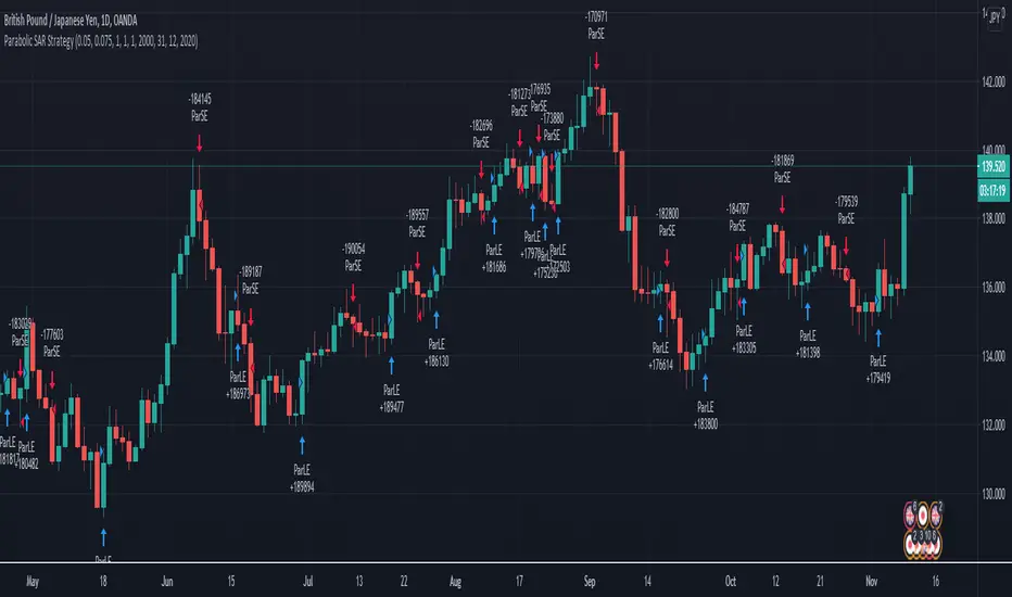
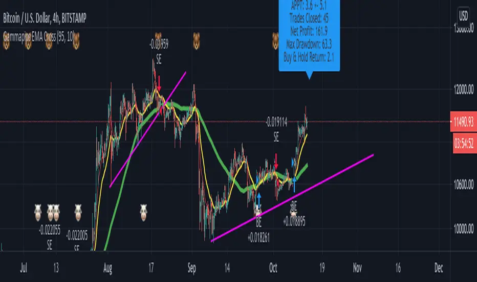
Top Strategy Finder [SpokoStocks]Top Strategy Finder
What if your chart could tell you which trading rule has actually worked on it?
Add this script to any symbol, any timeframe, and it backtests up to 2,304 complete strategies on that exact chart, ranks them, and shows a leaderboard you can read like a sentence: "Buy when RSI(2) drops below 10, only in calm volatility, exit on the reverse signal." Pick a row. Its trades appear on your price chart, its open position shows entry, stop and target, and its alerts are ready. No coding, no settings to tune.
Then it does something most strategy finders never show you: it walks forward and reports, without hindsight, whether trusting its own picks would have made money.
The problem it solves
Every strategy finder finds a winner. That is the easy part. Test enough rules on the same data and something always looks brilliant. The question that decides whether you make money is different: would that rule have worked from the moment you picked it?
This script answers it on the chart. On every bar it re-ranks all strategies using only the bars seen so far and follows a basket of the current leaders. The blue curve is what following those picks, bar by bar, would have produced. The gold curve is the champion's in-sample record. The gap between them is selection bias, drawn in the open. When both rise, the edge survived being chosen. When only the gold one does, you were looking at luck.
What you get
Leaderboard
• The top strategies (6 by default, up to 10) in plain language: entry on the first line, exit and filter on the second
• Trades and win rate as a bar, profit factor, net and max drawdown, all heat-coloured, in a table kept narrow so the chart stays visible
• Rank 1 starred, your selected row highlighted
• A trading plan for the selected row: exactly when to buy or sell, in which market condition, and how to exit
• A walk-forward line: what following the top basket would have earned, and how often the champion changed
• A "now" line: what your selected strategy and the basket hold on this bar
Performance pane
• Growth from the same start bar: buy & hold, the walk-forward basket, the champion, your selected row
• Each curve named with its result at the right edge
• Basket profit or loss area, optional drawdown shading, optional log scale
Price chart
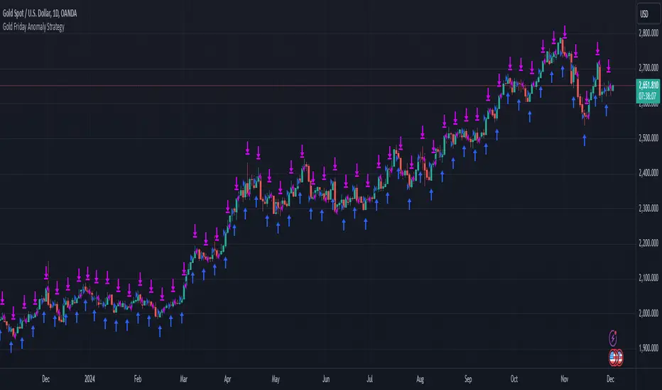
• The selected strategy's recent trades drawn as green or red segments
• Its open trade with entry, stop and target lines
• Exposure shading and markers whenever the followed strategy turns long, short or flat
Alerts
• Selected strategy enters long, enters short, exits
• Basket turns long or short
• Champion enters long or short, champion changed
What is tested
Each strategy = one entry signal × one direction × one exit rule × one market filter.
24 entries, each with a long and a mirrored short version: EMA 9/21 and 20/50 crosses · close crossing SMA 20 and SMA 50 · RSI(2) beyond 10/90 and 5/95 · RSI(14) leaving 30/70 and crossing 50 · close beyond the 2σ and 2.5σ Bollinger bands · 10, 20 and 55-bar breakouts · MACD histogram crossing zero · MACD line crossing signal · Supertrend (3,10) and (2,14) flips · Stochastic leaving 20/80 · inside-bar breakout · three closes against the trade · ADX above 20 with a DI cross · Williams %R beyond −90/−10 · fresh 10-bar extreme with a reversal close · gap continuation.
8 exits: after 5, 10 or 20 bars · stop 2 ATR / target 3 ATR · stop 1 ATR / target 2 ATR · stop and target 1.5 ATR · trailing stop 3 ATR · exit on the reverse signal.
6 filters: any market · with the 200-bar trend · against it · calm volatility · high volatility · with 20-bar momentum.
Search sizes: Quick 288 · Standard 768 · Deep 1,536 · Max 2,304.
How the backtest works
• Entries at the close of the signal bar.
• Stops and targets are checked against the following bars' highs and lows; if both are touched in one bar, the stop is assumed.
• Every side pays the cost you set (default 0.05%).
• A strategy must reach the minimum number of trades (default 30) and, by default, be net profitable to rank at all.
• Rank by Win %, SQN, profit factor, net profit, expectancy, return / drawdown, or average win / average loss.
• The champion keeps its title until a challenger beats it by a margin you set, so the title does not flip on noise.
• The walk-forward basket follows the top K (default 5) equally weighted, chosen at each bar's close and exposed to the next bar's move.
Repainting and data
All signals are evaluated on the chart's own OHLC data, with no higher-timeframe requests. Entries, exits and rankings are confirmed at the close of each bar; the walk-forward curve and every trade in the logs are built only from closed bars and do not change afterwards. The leaderboard order can change as new bars close, because new trades change the statistics; that is the ranking updating, not a redraw of history.
How to use it in five minutes
1. Add it to the chart you trade. Start with the Standard size.
2. Read the leaderboard. Favour rows with many trades and a modest drawdown over rows with a large net and few trades.
3. Look at the pane. Blue rising with gold: the edge survived being chosen. Blue flat while gold soars: the leaders are curve-fit to this chart.
4. Pick the row you want to trade. Read its plan under the table, check its drawn trades, set its alerts.
5. Switch the ranking metric. Rules that stay on top under several metrics are the robust ones.
What it is not
An indicator, not a strategy() script, so there is no order-by-order report from the built-in tester. It is a discovery tool: it tells you which rule to build and shows you, without hindsight, whether choosing that rule would have paid. Results depend on the bars tested (default the last 2,500) and on your cost setting. Past results do not guarantee future performance. This is not financial advice.
Indicatore

Momentum Sequence Strategy+ [Herman]Momentum Sequence Strategy is an open-source, rules-based price-action strategy designed to test momentum continuation following a defined candle sequence.
The strategy does not use moving averages, oscillators, volume indicators, or higher-timeframe data. Its signals are derived entirely from the relationship between consecutive OHLC candles.
The objective is to identify situations where an initial candle establishes a protected price extreme and is followed by a sequence of candles showing consistent momentum in the opposite direction.
How the strategy works
The model begins with a Main Candle, followed by a user-defined number of consecutive confirmation candles.
The number of following candles can be set to:
2
3
4
5
The default setting is 5 following candles.
Long setup
A Long setup requires:
The Main Candle to be bearish.
Every following candle to be bullish.
The low of every following candle must remain strictly above the low of the Main Candle.
Each new bullish candle must close higher than the previous bullish candle.
No position may already be open.
In simplified form:
Bearish Main Candle -> Bullish -> Bullish -> ... -> Long
The low of the Main Candle acts as the invalidation level for the sequence.
Short setup
The Short setup is the exact inverse of the Long setup.
A Short setup requires:
The Main Candle to be bullish.
Every following candle to be bearish.
The high of every following candle must remain strictly below the high of the Main Candle.
Each new bearish candle must close lower than the previous bearish candle.
No position may already be open.
In simplified form:
Bullish Main Candle -> Bearish -> Bearish -> ... -> Short
The high of the Main Candle acts as the invalidation level.
Long and Short trading can be enabled or disabled independently.
By default:
Long Trades: ON
Short Trades: OFF
The strategy allows only one open position at a time.
Stop Loss
For Long trades, the Stop Loss is placed at the low of the Main bearish Candle.
For Short trades, the Stop Loss is placed at the high of the Main bullish Candle.
This means the candle that begins the sequence defines the structural invalidation point of the trade.
Take Profit
The strategy uses configurable R-based targets:
0.5R / 1R / 1.5R / 2R
The default setting is 1.5R.
For a Long setup, risk is measured from the closing price of the final confirmation candle to the low of the Main Candle.
For a Short setup, risk is measured from the closing price of the final confirmation candle to the high of the Main Candle.
The selected R multiple is then applied to that distance to calculate the Take Profit level.
Important execution detail
The strategy identifies a completed sequence using confirmed candle data.
Under TradingView's standard historical strategy execution model, a market order generated after a confirmed bar will normally be filled on the next available tick, which is typically the open of the following bar.
The strategy calculates its R-based target using the close of the signal candle, rather than the eventual simulated market fill price.
Because of this, the selected 0.5R, 1R, 1.5R, or 2R setting represents the strategy's target calculation model and may not equal the exact realized risk-to-reward ratio measured from the simulated fill price. Gaps, market movement between bars, commissions, and slippage can further affect actual results.
Visuals
The strategy can display:
Long setup markers
Short setup markers
Active Stop Loss
Active Take Profit
A configurable statistics/settings table
The table displays the currently selected Take Profit, sequence length, and enabled trade directions.
Default configuration
The default script inputs are:
Following Candles: 5
Take Profit: 1.5R
Long Trades: ON
Short Trades: OFF
Entry Signals: ON
Stop Loss / Take Profit display: ON
These defaults are provided as a starting configuration for research and are not presented as optimized parameters for any particular market or timeframe.
Users are encouraged to evaluate different configurations across sufficiently large datasets rather than selecting parameters solely because they produced favorable historical results.
Intended use and limitations
This is a mechanical backtesting strategy intended for studying a specific candle-sequence behavior.
It does not evaluate market regime, trend, volatility, liquidity, volume, news events, session context, support/resistance, or other discretionary information.
A valid sequence therefore does not imply that a profitable trade will follow.
Historical strategy results are hypothetical and do not predict future performance. Results can vary materially depending on symbol, timeframe, trading costs, liquidity, execution assumptions, and selected parameters.
The strategy should be evaluated on standard price-based candlestick charts. Non-standard chart types such as Heikin Ashi, Renko, Range, Kagi, or Point & Figure can produce strategy results that do not correspond to tradable market prices.
This version extends that foundation with:
Pine Script v6 implementation
Configurable 2-5 candle sequence length
Mirrored Short-side logic
Independent Long/Short controls
Configurable R-based profit targets
One-position-at-a-time execution
Stop Loss and Take Profit visualization
Configurable on-chart settings table
Expanded user controls and documentation
The script is published open-source so users can inspect the complete methodology, verify its behavior, modify it, and conduct their own research. Strategia

ORB Laboratory v1.0.12ORB LABORATORY v1.0.12
Opening Range Breakout Research & Backtesting Framework
ORB Laboratory is a modular Opening Range Breakout strategy designed for systematic research, backtesting, robustness testing, and experimentation across different markets, sessions, symbols, timeframes, execution assumptions, and ORB methodologies.
This is not a single hard-coded ORB strategy.
The purpose of ORB Laboratory is to provide a flexible environment where traders and researchers can isolate individual variables, compare different approaches to opening-range behavior, and test whether an idea remains viable under different conditions rather than relying on one fixed set of rules.
The script includes multiple ORB sessions, seven entry models, configurable breakout buffers, several confirmation methods, market-condition filters, multiple stop-loss and profit-target models, position sizing, trade-frequency controls, execution modeling, breakeven and trailing-stop management, forced exits, and visual/debugging tools.
━━━━━━━━━━━━━━━━━━━━━━━━━━━━━━━━━━━━
1. MULTI-SESSION ORB ENGINE
━━━━━━━━━━━━━━━━━━━━━━━━━━━━━━━━━━━━
ORB Laboratory supports up to three independent Opening Range windows:
• ORB 1
• ORB 2
• ORB 3
Each ORB can be configured independently with:
• Enable / Disable
• Custom session name
• Starting hour
• Starting minute
• ORB duration in minutes
• Long trades enabled / disabled
• Short trades enabled / disabled
This makes it possible to research multiple market opens or intraday expansion periods within the same strategy.
Examples could include:
• New York open
• London open
• Secondary morning range
• Later-session expansion
• Crypto-specific session windows
• Custom event-based time windows
ORB lengths can range from very short opening ranges to much longer windows.
The strategy continuously tracks the highest high and lowest low while an ORB is forming.
When the ORB finishes, the final:
• ORB High
• ORB Low
• ORB Midpoint
are stored and projected forward on the chart.
The ORB is finalized on the close of the final range-building bar so resting breakout orders can be prepared before the first post-range bar begins.
The implementation also supports one-bar ORBs correctly.
━━━━━━━━━━━━━━━━━━━━━━━━━━━━━━━━━━━━
2. STRATEGY TIME ZONE
━━━━━━━━━━━━━━━━━━━━━━━━━━━━━━━━━━━━
The entire strategy uses a configurable strategy time zone.
This allows ORB sessions, entry cutoffs, forced closes, weekdays, and other time-sensitive logic to remain anchored to the desired market time regardless of the exchange or chart time zone.
Default:
America/New_York
━━━━━━━━━━━━━━━━━━━━━━━━━━━━━━━━━━━━
3. DIRECTION CONTROL
━━━━━━━━━━━━━━━━━━━━━━━━━━━━━━━━━━━━
Global direction can be set to:
• Both
• Long Only
• Short Only
Each individual ORB also has independent Long and Short permissions.
This means direction can be controlled both globally and per session.
━━━━━━━━━━━━━━━━━━━━━━━━━━━━━━━━━━━━
4. ENTRY ALLOWANCE / TRADE FREQUENCY
━━━━━━━━━━━━━━━━━━━━━━━━━━━━━━━━━━━━
ORB Laboratory includes several trade-frequency modes:
ONE TOTAL
Only one entry may be taken from an ORB.
ONCE PER DIRECTION
Allows one long and one short opportunity per ORB.
MAXIMUM NUMBER
Allows a configurable maximum number of entries per ORB.
UNLIMITED
Removes the per-ORB entry restriction while remaining subject to other global limits.
Additional controls include:
• Maximum entries per ORB
• Maximum entries per day
• Stop trading after first winning trade
• Stop trading after first losing trade
• Maximum planned daily risk
These tools make it possible to research whether an ORB performs better as a single-shot setup, one trade per direction, or as a multi-entry strategy.
━━━━━━━━━━━━━━━━━━━━━━━━━━━━━━━━━━━━
5. ENTRY MODEL — BREAKOUT (TOUCH)
━━━━━━━━━━━━━━━━━━━━━━━━━━━━━━━━━━━━
Breakout (Touch) is designed to model a traditional stop-order breakout.
After the ORB is complete, resting stop entries are prepared at:
Long:
ORB High + Long Breakout Buffer
Short:
ORB Low - Short Breakout Buffer
The entry can therefore occur when price touches the breakout threshold rather than waiting for a candle close.
The strategy uses resting stop orders for this mode.
Long and short breakout orders are placed into an OCA cancellation group.
When one side fills, competing unfilled breakout orders are cancelled.
This allows the strategy to model a two-sided opening-range breakout where both directions may initially be armed but only the triggered side remains active.
Unfilled Breakout (Touch) orders are also cancelled when the configured entry cutoff is reached.
━━━━━━━━━━━━━━━━━━━━━━━━━━━━━━━━━━━━
6. ENTRY MODEL — BREAKOUT (CLOSE)
━━━━━━━━━━━━━━━━━━━━━━━━━━━━━━━━━━━━
Breakout (Close) requires confirmation from the candle close.
Long:
Candle closes above the ORB High + Long Breakout Buffer.
Short:
Candle closes below the ORB Low - Short Breakout Buffer.
This model is useful for comparing immediate touch-based breakout execution against the additional confirmation of a completed candle outside the range.
━━━━━━━━━━━━━━━━━━━━━━━━━━━━━━━━━━━━
7. ENTRY MODEL — BREAK + RETEST ORB
━━━━━━━━━━━━━━━━━━━━━━━━━━━━━━━━━━━━
This model waits for a confirmed breakout and then looks for price to retest the broken ORB boundary.
After a breakout, the retest can be confirmed using one of three methods:
TOUCH ONLY
Price only needs to return to the broken ORB boundary.
CLOSE OUTSIDE
Price must retest the boundary and close back on the breakout side.
REJECTION CANDLE
Price must retest the boundary and produce directional rejection.
For a bullish retest, the candle must interact with the ORB High and confirm back above it.
For a bearish retest, the candle must interact with the ORB Low and confirm back below it.
Additional controls include:
• Retest expiry in bars
• Maximum extension before a retest is considered too late
Once a valid retest is consumed, the retest setup is disarmed.
━━━━━━━━━━━━━━━━━━━━━━━━━━━━━━━━━━━━
8. ENTRY MODEL — BREAK + RETEST FVG
━━━━━━━━━━━━━━━━━━━━━━━━━━━━━━━━━━━━
ORB Laboratory includes directional Fair Value Gap detection following an ORB breakout.
A bullish FVG is detected when a three-candle imbalance exists with the current low above the high from two bars earlier.
A bearish FVG is detected when the current high is below the low from two bars earlier.
The minimum FVG size can be defined as an ATR multiple.
Optional logic can require the FVG to remain outside the ORB.
Three FVG entry depths are available:
NEAR EDGE
Uses the first edge of the FVG encountered on the retracement.
MIDPOINT
Uses the 50% level of the FVG.
FULL FILL
Requires price to reach the opposite edge of the FVG.
Additional controls include:
• Minimum FVG size as ATR ×
• FVG must remain outside ORB
• FVG expiry in bars
If price reaches the selected FVG level while the setup is valid, an entry is submitted in the direction of the original breakout.
━━━━━━━━━━━━━━━━━━━━━━━━━━━━━━━━━━━━
9. ENTRY MODEL — SWEEP REVERSAL
━━━━━━━━━━━━━━━━━━━━━━━━━━━━━━━━━━━━
Sweep Reversal is designed to research failed breaks of the opening range.
A high sweep occurs when price trades above:
ORB High + Long Breakout Buffer
but then closes back below the ORB High.
A low sweep occurs when price trades below:
ORB Low - Short Breakout Buffer
but then closes back above the ORB Low.
Two confirmation modes are available:
CLOSE BACK INSIDE
The breakout only needs to fail and close back inside the ORB.
REJECTION CANDLE
The failed breakout must also produce a directional rejection candle.
A failed high produces a potential short setup.
A failed low produces a potential long setup.
Sweep trades are treated as fade/reversal trades and can use dedicated fade-target logic.
━━━━━━━━━━━━━━━━━━━━━━━━━━━━━━━━━━━━
10. ENTRY MODEL — FADE FIRST BREAKOUT
━━━━━━━━━━━━━━━━━━━━━━━━━━━━━━━━━━━━
This model records which side of the ORB breaks first.
The strategy permanently tracks:
• First breakout direction
• First breakout bar
• Maximum extension reached by that breakout
If the first breakout subsequently fails and closes back inside the ORB within the configured failure window, the strategy can fade that failed move.
First high breakout fails:
Potential short.
First low breakout fails:
Potential long.
The model also includes a Maximum Extension Before Retest/Fade setting.
This prevents an extremely extended move from later being treated as a normal failed breakout simply because price eventually returns to the range.
A configurable First-Break Failure Timeout controls how many bars the setup remains eligible.
━━━━━━━━━━━━━━━━━━━━━━━━━━━━━━━━━━━━
11. ENTRY MODEL — FIRST-BREAK DECISION TREE
━━━━━━━━━━━━━━━━━━━━━━━━━━━━━━━━━━━━
The First-Break Decision Tree is a hybrid model that evaluates what happens after the first ORB break.
Instead of automatically assuming that the first breakout should either be followed or faded, the script waits to determine whether the move confirms continuation or fails.
The first breakout direction and extreme are recorded.
Continuation can then be defined as:
TOUCH
Price reaches the breakout threshold.
CLOSE OUTSIDE
Price closes outside the ORB in the breakout direction.
RETEST HOLDS
Price retests the broken boundary and closes back on the breakout side.
If continuation confirms, the strategy trades in the direction of the original breakout.
If the first breakout instead fails and closes back inside the ORB during the allowed failure window, the strategy can reverse and trade against the failed breakout.
This allows a single model to test both:
• Breakout continuation
• Failed-break reversal
using the first interaction with the opening range as the decision point.
━━━━━━━━━━━━━━━━━━━━━━━━━━━━━━━━━━━━
12. BREAKOUT BUFFER SYSTEM
━━━━━━━━━━━━━━━━━━━━━━━━━━━━━━━━━━━━
Long and short breakout buffers are independently configurable.
Buffers can be expressed using:
TICKS
Buffer is based on the symbol's minimum tick size.
ORB %
Buffer is calculated as a percentage of the completed ORB range.
ATR
Buffer is calculated as a multiple of ATR.
This allows breakout confirmation to be normalized in several different ways.
For example, researchers can test whether a fixed one-tick breakout behaves differently from a volatility-adjusted or range-adjusted breakout.
━━━━━━━━━━━━━━━━━━━━━━━━━━━━━━━━━━━━
13. BID / ASK TRIGGER MODEL
━━━━━━━━━━━━━━━━━━━━━━━━━━━━━━━━━━━━
Breakout (Touch) includes an optional bid/ask trigger-timing model.
Application can be set to:
• Off
• Longs Only
• Shorts Only
• Both
Spread can be entered as:
• Ticks
• Absolute price
The model allows the visible TradingView trigger to be shifted relative to the intended execution level.
For example, on a bid-based chart, a long ask-trigger may occur while the visible bid remains one spread below the intended buy price.
The model therefore allows researchers to approximate the difference between:
• Structural/intended execution level
• Visible chart trigger level
IMPORTANT:
TradingView Strategy Tester still records the chart-trigger price as the actual historical fill.
Because of this limitation, built-in Strategy Tester P&L remains an approximation when bid/ask trigger modeling is enabled.
The feature is intended for execution research and timing approximation, not as a claim of perfect historical bid/ask reconstruction.
━━━━━━━━━━━━━━━━━━━━━━━━━━━━━━━━━━━━
14. BID / ASK STOP MODEL
━━━━━━━━━━━━━━━━━━━━━━━━━━━━━━━━━━━━
ORB Laboratory separately includes a spread model for stop-loss triggering.
Application options include:
• Off
• Long Stops Only
• Short Stops Only
• Both
This allows the displayed TradingView stop trigger to be shifted relative to the structural stop by the modeled spread.
The structural stop itself is still retained internally for calculations when desired.
This makes the entry-side spread assumption and stop-side spread assumption independently configurable.
━━━━━━━━━━━━━━━━━━━━━━━━━━━━━━━━━━━━
15. ENTRY CALCULATION PRICE
━━━━━━━━━━━━━━━━━━━━━━━━━━━━━━━━━━━━
When spread modeling is active, Fixed-R calculations can use either:
CORRECTED ENTRY
Uses the intended execution level.
CHART TRIGGER
Uses the spread-shifted TradingView trigger.
This setting affects Fixed-R target calculations.
It does not independently change the actual submitted quantity or order execution.
━━━━━━━━━━━━━━━━━━━━━━━━━━━━━━━━━━━━
16. STOP CALCULATION PRICE
━━━━━━━━━━━━━━━━━━━━━━━━━━━━━━━━━━━━
Risk calculations can use either:
CORRECTED STOP
Uses the modeled spread-adjusted stop.
ORIGINAL STOP
Uses the underlying structural stop.
This selection can affect:
• Position sizing
• Original risk calculation
• Fixed-R target calculations
This allows researchers to separate structural price levels from the levels used to approximate executable stop behavior.
━━━━━━━━━━━━━━━━━━━━━━━━━━━━━━━━━━━━
17. EMA FILTER
━━━━━━━━━━━━━━━━━━━━━━━━━━━━━━━━━━━━
An optional EMA directional filter is included.
The EMA length is configurable.
Available rules:
PRICE VS EMA
Long:
Price must be above the EMA.
Short:
Price must be below the EMA.
EMA SLOPE
Long:
EMA must be rising.
Short:
EMA must be falling.
BOTH
Requires both the appropriate price relationship and EMA slope.
When enabled, the EMA is also plotted on the chart.
━━━━━━━━━━━━━━━━━━━━━━━━━━━━━━━━━━━━
18. VWAP FILTER
━━━━━━━━━━━━━━━━━━━━━━━━━━━━━━━━━━━━
An optional VWAP directional filter is available.
Rules include:
PRICE VS VWAP
Long:
Price above VWAP.
Short:
Price below VWAP.
VWAP SLOPE
Long:
VWAP rising.
Short:
VWAP falling.
BOTH
Requires both conditions.
When enabled, VWAP is plotted directly on the chart.
━━━━━━━━━━━━━━━━━━━━━━━━━━━━━━━━━━━━
19. PREVIOUS CLOSE FILTER
━━━━━━━━━━━━━━━━━━━━━━━━━━━━━━━━━━━━
The script retrieves the confirmed previous daily close without lookahead.
Two filtering modes are available:
PRICE VS PREVIOUS CLOSE
Long:
Current price must be above the previous close.
Short:
Current price must be below the previous close.
ORB VS PREVIOUS CLOSE
Long:
The entire ORB must be above the previous close.
Short:
The entire ORB must be below the previous close.
━━━━━━━━━━━━━━━━━━━━━━━━━━━━━━━━━━━━
20. ORB RANGE FILTER
━━━━━━━━━━━━━━━━━━━━━━━━━━━━━━━━━━━━
A configurable minimum and maximum ORB range filter is included.
The ORB size can be measured in:
• Ticks
• ATR multiples
• Percentage of price
This allows researchers to reject ranges that are considered:
• Too small
• Too large
• Abnormally compressed
• Abnormally volatile
It also makes range thresholds more portable across different symbols and volatility environments.
━━━━━━━━━━━━━━━━━━━━━━━━━━━━━━━━━━━━
21. RELATIVE VOLUME FILTER
━━━━━━━━━━━━━━━━━━━━━━━━━━━━━━━━━━━━
An optional relative-volume condition compares current volume with a moving average of volume.
Controls include:
• Volume average length
• Minimum relative-volume multiplier
A trade is permitted only when current volume meets or exceeds the selected multiple of average volume.
━━━━━━━━━━━━━━━━━━━━━━━━━━━━━━━━━━━━
22. ADX FILTER
━━━━━━━━━━━━━━━━━━━━━━━━━━━━━━━━━━━━
An optional ADX filter is included.
Controls:
• ADX length
• Minimum ADX value
This can be used to research whether ORB setups behave differently during stronger or weaker directional conditions.
━━━━━━━━━━━━━━━━━━━━━━━━━━━━━━━━━━━━
23. MAXIMUM BREAKOUT CANDLE SIZE
━━━━━━━━━━━━━━━━━━━━━━━━━━━━━━━━━━━━
The strategy can reject entry conditions when the current candle becomes excessively large relative to ATR.
Maximum breakout candle size is expressed as:
ATR × multiplier
This can be used to study whether chasing unusually extended breakout candles damages expectancy.
━━━━━━━━━━━━━━━━━━━━━━━━━━━━━━━━━━━━
24. STOP LOSS — CANDLE EXTREME
━━━━━━━━━━━━━━━━━━━━━━━━━━━━━━━━━━━━
For long trades:
Stop is placed below the relevant candle low, with an optional tick buffer.
For short trades:
Stop is placed above the relevant candle high, with an optional tick buffer.
━━━━━━━━━━━━━━━━━━━━━━━━━━━━━━━━━━━━
25. STOP LOSS — ATR
━━━━━━━━━━━━━━━━━━━━━━━━━━━━━━━━━━━━
Places the stop a configurable ATR distance from the entry/reference price.
Long:
Entry/reference price - ATR × multiplier
Short:
Entry/reference price + ATR × multiplier
━━━━━━━━━━━━━━━━━━━━━━━━━━━━━━━━━━━━
26. STOP LOSS — ORB MIDPOINT
━━━━━━━━━━━━━━━━━━━━━━━━━━━━━━━━━━━━
Uses the midpoint between the ORB High and ORB Low as the structural stop.
━━━━━━━━━━━━━━━━━━━━━━━━━━━━━━━━━━━━
27. STOP LOSS — ORB OPPOSITE RANGE
━━━━━━━━━━━━━━━━━━━━━━━━━━━━━━━━━━━━
Long:
Stop below the ORB Low.
Short:
Stop above the ORB High.
An optional stop buffer in ticks can be applied beyond the opposite boundary.
━━━━━━━━━━━━━━━━━━━━━━━━━━━━━━━━━━━━
28. STOP LOSS — BREAKOUT EXTREME
━━━━━━━━━━━━━━━━━━━━━━━━━━━━━━━━━━━━
Uses the relevant breakout extreme as the stop reference, with the optional stop buffer applied beyond that level.
This is useful for retest, failure, sweep, and other models where the breakout structure itself provides the invalidation point.
━━━━━━━━━━━━━━━━━━━━━━━━━━━━━━━━━━━━
29. STOP LOSS — ORB PERCENTAGE
━━━━━━━━━━━━━━━━━━━━━━━━━━━━━━━━━━━━
Stop distance is calculated as a configurable percentage of the completed ORB range.
This allows the stop distance to scale directly with the size of the opening range.
━━━━━━━━━━━━━━━━━━━━━━━━━━━━━━━━━━━━
30. STOP LOSS — FVG INVALIDATION
━━━━━━━━━━━━━━━━━━━━━━━━━━━━━━━━━━━━
Uses the relevant FVG boundary as the stop reference.
Long:
Below the FVG bottom.
Short:
Above the FVG top.
The configured stop buffer may also be applied.
━━━━━━━━━━━━━━━━━━━━━━━━━━━━━━━━━━━━
31. STOP BUFFER
━━━━━━━━━━━━━━━━━━━━━━━━━━━━━━━━━━━━
A configurable stop buffer can be added in ticks.
This allows the structural stop to sit beyond the selected invalidation level rather than directly on it.
━━━━━━━━━━━━━━━━━━━━━━━━━━━━━━━━━━━━
32. PROFIT TARGET — FIXED R
━━━━━━━━━━━━━━━━━━━━━━━━━━━━━━━━━━━━
Profit target is calculated as a multiple of the original trade risk.
Long:
Entry + Risk × R Multiple
Short:
Entry - Risk × R Multiple
The R multiple is fully configurable.
━━━━━━━━━━━━━━━━━━━━━━━━━━━━━━━━━━━━
33. PROFIT TARGET — ORB PROJECTION
━━━━━━━━━━━━━━━━━━━━━━━━━━━━━━━━━━━━
Projects a configurable multiple of the complete ORB range beyond the breakout boundary.
Long:
ORB High + ORB Range × multiplier
Short:
ORB Low - ORB Range × multiplier
━━━━━━━━━━━━━━━━━━━━━━━━━━━━━━━━━━━━
34. PROFIT TARGET — ATR
━━━━━━━━━━━━━━━━━━━━━━━━━━━━━━━━━━━━
Sets the target a configurable ATR multiple away from entry.
Long:
Entry + ATR × multiplier
Short:
Entry - ATR × multiplier
━━━━━━━━━━━━━━━━━━━━━━━━━━━━━━━━━━━━
35. PROFIT TARGET — ORB MIDPOINT
━━━━━━━━━━━━━━━━━━━━━━━━━━━━━━━━━━━━
Uses the ORB midpoint as the target.
This can be useful when researching reversal or mean-reversion behavior.
━━━━━━━━━━━━━━━━━━━━━━━━━━━━━━━━━━━━
36. PROFIT TARGET — ORB OPPOSITE RANGE
━━━━━━━━━━━━━━━━━━━━━━━━━━━━━━━━━━━━
Targets the opposite ORB boundary.
This is especially useful for studying moves that rotate from one side of the range toward the other.
━━━━━━━━━━━━━━━━━━━━━━━━━━━━━━━━━━━━
37. DEDICATED FADE TARGETS
━━━━━━━━━━━━━━━━━━━━━━━━━━━━━━━━━━━━
Fade/reversal entries can use their own target preference:
• Midpoint
• Opposite Boundary
• Fixed R
This allows continuation trades and fade trades to be researched using different exit logic.
━━━━━━━━━━━━━━━━━━━━━━━━━━━━━━━━━━━━
38. POSITION SIZING — FIXED USD RISK
━━━━━━━━━━━━━━━━━━━━━━━━━━━━━━━━━━━━
Position size can be calculated so the planned loss between entry and stop corresponds to a fixed dollar amount.
The script calculates:
• Entry-to-stop distance
• Cash risk per unit
• Required quantity
and then rounds quantity according to the configured quantity step.
━━━━━━━━━━━━━━━━━━━━━━━━━━━━━━━━━━━━
39. POSITION SIZING — RISK % OF EQUITY
━━━━━━━━━━━━━━━━━━━━━━━━━━━━━━━━━━━━
Position size can dynamically scale with strategy equity.
The selected percentage of current equity is divided by the calculated cash risk per unit to determine quantity.
This allows compounding-based position sizing to be researched.
━━━━━━━━━━━━━━━━━━━━━━━━━━━━━━━━━━━━
40. POSITION SIZING — FIXED QUANTITY
━━━━━━━━━━━━━━━━━━━━━━━━━━━━━━━━━━━━
A fixed position size can be used instead of risk-based sizing.
━━━━━━━━━━━━━━━━━━━━━━━━━━━━━━━━━━━━
41. QUANTITY CONSTRAINTS
━━━━━━━━━━━━━━━━━━━━━━━━━━━━━━━━━━━━
Position sizing supports:
• Quantity step
• Minimum quantity
• Maximum quantity
Calculated quantity is stepped downward to the permitted increment and then constrained within the configured minimum and maximum.
This makes sizing adaptable to instruments with different contract or quantity requirements.
━━━━━━━━━━━━━━━━━━━━━━━━━━━━━━━━━━━━
42. MAXIMUM DAILY PLANNED RISK
━━━━━━━━━━━━━━━━━━━━━━━━━━━━━━━━━━━━
An optional daily planned-risk ceiling can prevent new entries when another planned trade would push total daily risk above the configured limit.
A value of zero disables this restriction.
━━━━━━━━━━━━━━━━━━━━━━━━━━━━━━━━━━━━
43. STOP AFTER FIRST WIN
━━━━━━━━━━━━━━━━━━━━━━━━━━━━━━━━━━━━
When enabled, the strategy prevents further entries after the first profitable closed trade of the day.
━━━━━━━━━━━━━━━━━━━━━━━━━━━━━━━━━━━━
44. STOP AFTER FIRST LOSS
━━━━━━━━━━━━━━━━━━━━━━━━━━━━━━━━━━━━
When enabled, the strategy prevents further entries after the first losing closed trade of the day.
These two controls can be used independently to study daily stopping rules.
━━━━━━━━━━━━━━━━━━━━━━━━━━━━━━━━━━━━
45. ENTRY CUTOFF
━━━━━━━━━━━━━━━━━━━━━━━━━━━━━━━━━━━━
A configurable time prevents new entries after a chosen hour and minute.
For Breakout (Touch), any remaining unfilled resting breakout orders are cancelled when the cutoff is reached.
━━━━━━━━━━━━━━━━━━━━━━━━━━━━━━━━━━━━
46. FORCE CLOSE
━━━━━━━━━━━━━━━━━━━━━━━━━━━━━━━━━━━━
An optional forced-close time exits any remaining open position at or after the configured time.
This is useful for strictly intraday strategies that should not carry positions beyond a session boundary.
━━━━━━━━━━━━━━━━━━━━━━━━━━━━━━━━━━━━
47. WEEKDAY FILTERS
━━━━━━━━━━━━━━━━━━━━━━━━━━━━━━━━━━━━
Every day of the week can be independently enabled or disabled:
• Monday
• Tuesday
• Wednesday
• Thursday
• Friday
• Saturday
• Sunday
This allows weekday effects to be researched without modifying the strategy code.
━━━━━━━━━━━━━━━━━━━━━━━━━━━━━━━━━━━━
48. BREAKEVEN MANAGEMENT
━━━━━━━━━━━━━━━━━━━━━━━━━━━━━━━━━━━━
An optional breakeven system can move the active stop after price reaches a configurable R multiple.
Controls:
• Breakeven activation R
• Breakeven offset in ticks
For a long position, the stop can move to entry plus the selected offset.
For a short position, the stop can move to entry minus the selected offset.
The stop is only tightened; the logic does not intentionally loosen an existing stop.
━━━━━━━━━━━━━━━━━━━━━━━━━━━━━━━━━━━━
49. BAR-CLOSE ATR TRAILING STOP
━━━━━━━━━━━━━━━━━━━━━━━━━━━━━━━━━━━━
An optional ATR trailing system activates after the trade reaches a configurable R threshold.
The strategy tracks the best confirmed close reached during the trade.
After activation:
Long:
Trail candidate = Best Close - Entry ATR × Trail Multiplier
Short:
Trail candidate = Best Close + Entry ATR × Trail Multiplier
The stop only ratchets in the favorable direction.
The trailing logic operates on confirmed bars.
━━━━━━━━━━━━━━━━━━━━━━━━━━━━━━━━━━━━
50. TIME-BASED EXIT
━━━━━━━━━━━━━━━━━━━━━━━━━━━━━━━━━━━━
Positions can optionally be closed after a specified number of bars.
Setting the value to zero disables the time exit.
━━━━━━━━━━━━━━━━━━━━━━━━━━━━━━━━━━━━
51. ONE ACTIVE POSITION / NO PYRAMIDING
━━━━━━━━━━━━━━━━━━━━━━━━━━━━━━━━━━━━
The strategy is configured with pyramiding disabled.
New setups also require the strategy to be flat before entry.
This keeps the framework focused on one active position at a time rather than stacking multiple simultaneous positions.
━━━━━━━━━━━━━━━━━━━━━━━━━━━━━━━━━━━━
52. OCA BREAKOUT ORDER MANAGEMENT
━━━━━━━━━━━━━━━━━━━━━━━━━━━━━━━━━━━━
Breakout (Touch) orders use One-Cancels-All behavior.
When one resting breakout order fills, competing unfilled touch orders are cancelled.
The strategy then records the filled ORB, direction, stop, target, entry ATR, and original risk for active position management.
━━━━━━━━━━━━━━━━━━━━━━━━━━━━━━━━━━━━
53. ORB VISUALIZATION
━━━━━━━━━━━━━━━━━━━━━━━━━━━━━━━━━━━━
Optional ORB boxes display the opening-range construction directly on the chart.
Once complete, the script extends:
• ORB High
• ORB Low
• Optional ORB Midpoint
forward on the chart.
This allows the strategy logic to be inspected visually rather than only through Strategy Tester results.
━━━━━━━━━━━━━━━━━━━━━━━━━━━━━━━━━━━━
54. SIGNAL LABELS
━━━━━━━━━━━━━━━━━━━━━━━━━━━━━━━━━━━━
Optional labels identify strategy entries and their originating logic.
Examples include:
• Breakout Touch Fill
• Breakout Close
• ORB Retest
• FVG Retest
• High Sweep
• Low Sweep
• Fade First High Break
• Fade First Low Break
• Decision: Continuation
• Decision: Failed High
• Decision: Failed Low
━━━━━━━━━━━━━━━━━━━━━━━━━━━━━━━━━━━━
55. BLOCKED-REASON DEBUGGING
━━━━━━━━━━━━━━━━━━━━━━━━━━━━━━━━━━━━
Optional debugging labels can show why an otherwise evaluated setup was blocked.
Possible reasons include:
• Direction disabled
• Range filter
• Entry / daily limit
• Bias / condition filter
• Other blocked condition
This feature is designed to make strategy research easier by showing not only where entries occurred, but also why expected entries did not occur.
━━━━━━━━━━━━━━━━━━━━━━━━━━━━━━━━━━━━
56. ACTIVE STOP & TARGET PLOTS
━━━━━━━━━━━━━━━━━━━━━━━━━━━━━━━━━━━━
While a position is open, the strategy can display:
• Active Stop
• Active Target
directly on the chart.
Stops dynamically reflect breakeven or trailing-stop adjustments when those systems are active.
━━━━━━━━━━━━━━━━━━━━━━━━━━━━━━━━━━━━
57. RESEARCH DASHBOARD
━━━━━━━━━━━━━━━━━━━━━━━━━━━━━━━━━━━━
An optional dashboard displays current strategy information including:
• Selected Entry Model
• Daily Entries vs Maximum
• Planned Daily Risk
• EMA Bias
• VWAP Bias
• Previous Daily Close
• Current Position: Long / Short / Flat
• Entry Cutoff Time
The dashboard provides a compact view of the currently active configuration and state.
━━━━━━━━━━━━━━━━━━━━━━━━━━━━━━━━━━━━
58. PREVIOUS DAILY CLOSE WITHOUT LOOKAHEAD
━━━━━━━━━━━━━━━━━━━━━━━━━━━━━━━━━━━━
The previous-close feature retrieves confirmed daily data using lookahead disabled and then references the prior confirmed daily close.
This avoids intentionally using future daily information in the previous-close filter.
━━━━━━━━━━━━━━━━━━━━━━━━━━━━━━━━━━━━
59. RESEARCH-FIRST DESIGN
━━━━━━━━━━━━━━━━━━━━━━━━━━━━━━━━━━━━
ORB Laboratory is intentionally modular.
Many settings are not intended to be enabled simultaneously.
The purpose is to allow individual hypotheses to be isolated.
Examples:
• Does Touch outperform Close confirmation?
• Does requiring a retest improve expectancy?
• Are failed first breaks more useful as fades?
• Does the ORB midpoint outperform an ATR stop?
• Does an EMA or VWAP filter improve results?
• Are very small or very large ORBs less effective?
• Does a breakout buffer improve robustness?
• Does performance survive different stop models?
• Does Fixed-R outperform range projection?
• How sensitive are results to spread assumptions?
• How does limiting entries affect drawdown?
• Do certain weekdays behave differently?
• Does breakeven improve or damage expectancy?
The framework is designed to answer those questions with data rather than intuition.
━━━━━━━━━━━━━━━━━━━━━━━━━━━━━━━━━━━━
IMPORTANT BACKTESTING NOTES
━━━━━━━━━━━━━━━━━━━━━━━━━━━━━━━━━━━━
ORB Laboratory is a research and backtesting tool.
Historical results can change significantly based on:
• Symbol
• Exchange / broker data feed
• Timeframe
• ORB session
• ORB length
• Entry model
• Breakout buffer
• Stop model
• Target model
• Position sizing
• Spread assumptions
• Commission
• Slippage
• Filters
• Test period
• Market regime
Different data feeds can produce different highs and lows and therefore different ORB boundaries, triggers, stops, targets, and trade sequences.
Results from one feed should not be assumed to reproduce another feed trade-for-trade.
The optional bid/ask modeling system is an approximation built around TradingView's historical-chart limitations.
TradingView may still report the chart trigger as the historical fill even when the strategy is using a corrected/intended price internally for risk or target calculations.
Users should configure TradingView's Strategy Properties appropriately for the instrument and execution assumptions being researched, including commissions and any additional slippage assumptions.
No backtest guarantees future results.
━━━━━━━━━━━━━━━━━━━━━━━━━━━━━━━━━━━━
INTENDED USE
━━━━━━━━━━━━━━━━━━━━━━━━━━━━━━━━━━━━
ORB Laboratory is intended for:
• Strategy research
• Backtesting
• Robustness testing
• Parameter sensitivity testing
• Comparing ORB entry models
• Comparing stop and target logic
• Studying opening-range behavior
• Execution-model research
• Market and data-feed comparison
• Educational experimentation
It is not intended to provide financial advice, guaranteed signals, or guaranteed profitability.
A profitable historical configuration may fail in future market conditions.
Users should independently validate any configuration before considering live execution.
Build the range.
Define the rules.
Stress the assumptions.
Test the edge. Strategia

Strategy Forecast EngineThe Strategy Forecast Engine is a regime-based Monte Carlo forecasting tool that estimates the future return distribution of trend-following strategies across different market environments. The model identifies the current market regime, conditions forecasts on historical returns observed during comparable regimes, and generates thousands of potential future price paths using Monte Carlo simulation. The resulting return distribution is presented through percentile projections and a structured, color-coded table that provides a comprehensive assessment of the forecast.
First, the model identifies the current market regime using the selected trend-following strategy. Users can choose between a moving-average crossover strategy, a volatility-based trailing stop strategy, or a combined strategy that incorporates both approaches. Supported moving-average types include the Exponential Moving Average (EMA), Simple Moving Average (SMA), Wilder’s Moving Average (RMA), and Weighted Moving Average (WMA). Supported volatility types include the Average True Range (ATR), Standard Deviation (SD), and Mean Absolute Deviation (MAD). By default, the model applies an asymmetric design in which conflicting signals default to bullish unless neutral regimes are enabled in the menu. Market regimes are determined as follows:
Bullish Trend Regime = (Fast MA – Slow MA) > (ATR × Trend Margin)
Bearish Trend Regime = (Fast MA – Slow MA) < –(ATR × Trend Margin)
Bullish Volatility Regime = Price > (Highest Price – (Volatility × Stop Factor))
Bearish Volatility Regime = Price < (Lowest Price + (Volatility × Stop Factor))
Bullish Combined Regime = Bullish Trend Regime and Bullish Volatility Regime
Bearish Combined Regime = Bearish Trend Regime and Bearish Volatility Regime
Once the current regime has been identified, the model collects all historical logarithmic returns that occurred during the same regime beginning from the selected start date. Only returns from the matching regime are used to generate the forecast, allowing projections to be conditioned on historically comparable market environments rather than treating all historical observations as equally relevant. If duration-adjusted forecast is enabled in the menu, the model further restricts the sample pool to returns from regimes that were at least as mature as the current regime.
The Monte Carlo simulation engine then generates thousands of possible future price paths over the selected forecast horizon. Each simulation randomly samples historical returns from the sample pool associated with the current regime and compounds them forward to generate a potential future price path. This process is repeated for the specified number of simulations to produce a broad range of possible future outcomes. The random seed controls reproducibility, ensuring that identical settings produce identical forecasts. Once all individual simulations have been completed, the resulting return distribution is summarized using percentile projections:
95% = 5% of simulations ended above this level and 95% ended below it.
75% = 25% of simulations ended above this level and 75% ended below it.
Median = 50% of simulations ended above this level and 50% ended below it.
25% = 25% of simulations ended below this level and 75% ended above it.
5% = 5% of simulations ended below this level and 95% ended above it.
The upper quartile (75%) and lower quartile (25%) define the Interquartile Range (IQR), which contains the middle 50% of all simulated outcomes and represents the central range of the projected outcome distribution. The upper and lower tail percentiles can be set to 10% (90% / 10%), 5% (95% / 5%), or 1% (99% / 1%). The default setting is 5%, which captures the middle 90% of simulated outcomes. At 10%, the range captures 80% of simulated outcomes, while at 1%, the range captures 98% of simulated outcomes. To further evaluate the risk/reward characteristics of the forecast, the model includes a built-in table with the following metrics:
Regime = Current market regime based on the selected strategy configuration.
Duration = Percentile rank of current regime duration relative to past regimes.
Forecast = Percentile rank of current duration including the forecast horizon.
Win Rate = Percentage of profitable simulations relative to total simulations.
Profit Factor = Ratio of total simulated profits to total simulated losses.
Expectancy = Average expected percentage return across all simulations.
Reward/Risk = Ratio of upper quartile return to lower quartile return.
Asymmetry = Ratio of selected upper tail return to selected lower tail return.
Skewness = Ratio of upside potential to downside risk relative to the median.
Sample Size = Number of historical returns available for the current regime.
Frequency = Percentage of historical returns belonging to the current regime.
In summary, the Strategy Forecast Engine is a comprehensive forecasting tool designed to help investors evaluate the return distribution of trend-following strategies based on the current market regime. By combining regime detection with Monte Carlo simulation, the model conditions forecasts on historical returns observed during comparable market regimes to estimate the distribution of potential outcomes and their associated risk/reward characteristics. While the model provides valuable insight into historical return patterns, investors should remain mindful that historical market behavior may not necessarily persist under future market conditions. Indicatore

[3Commas] UNI Vault Grid - UNI - Indicator UNI Vault Grid — UNI — Indicator
🔷 What it does:
This indicator is the visual + signal-only companion to the static geometric grid strategy for Uniswap (UNI/USDT). It draws all 57 grid levels on the chart, fires Buy and Sell signals on each close-cross event, tracks a virtual P&L card (simulating what the matching strategy would have done), and ships webhook alerts for routing signals to a connected grid bot. Use it when you want the grid logic running on your chart without strategy.* engine — for visual confirmation, manual entries, or external bot routing.
- 57 geometrically-spaced levels between Low (2.979) and High (4.171) drawn as horizontal lines
- Buy / Sell labels printed at each level on cross events
- Virtual P&L tracker mirrors the strategy version's bookkeeping
- Static range — grid does NOT shift up when price exits the band (trailing-up disabled)
- Webhook-ready alert payload for connected grid bot
🔷 Who is it for:
Traders who want to visualize the grid and signal layer on their chart without running the strategy engine.
Bot operators routing signals from TradingView alerts to a connected grid bot via webhook.
Discretionary swing traders who want grid levels as decision support while executing manually.
Users comparing live signal flow against backtested behavior of the matching strategy publication.
🔷 How does it work:
Grid Construction: On the first bar, the indicator pre-computes 57 price levels between Low (2.979) and High (4.171) using geometric spacing (≈ 0.61% step). Each level is drawn as a horizontal line — green for the lowest, red for the highest, aqua for the middle levels.
Signal Generation: On every confirmed bar, the indicator checks each level for a close-cross-down (Buy signal) or close-cross-up (Sell signal) against the next level above. A label is printed at the level on each cross. Buy labels are aqua, Sell labels are fuchsia and include the realized virtual P&L.
Virtual P&L Tracker: The indicator maintains its own bookkeeping that mirrors the strategy version — when a Buy level fills, qty is recorded; when the next-up Sell level crosses, the per-level P&L is added to the virtual net. Stats card displays Net P&L, Max Drawdown, Total Fills, Win Rate, and Profit Factor.
Webhook Alerts: A grid_start JSON payload (Bot ID, Email Token, Pair) is fired once when the first bar enters the configured backtest window. This is informational — grid bots are typically configured on the bot interface directly.
🔷 Why it's unique:
Identical grid math to the strategy publication — same 57 levels, same step, same cross-detection logic. The virtual P&L card lets you see live what the strategy version is doing in backtest, but on an indicator pane (no strategy.* engine, no order fills).
Static range fidelity — no trailing-up. The grid stays locked exactly where you configured it, which makes risk envelope easy to reason about before deploying capital.
Brand watermark + stats overlay — consistent visual layer with all other 3Commas Vault Grid publications.
🔷 Considerations Before Using the Indicator:
Market & Timeframe: Calibrated for a 15-minute chart on UNI/USDT spot pairs. The runtime warning label flags any TF other than 15m. Higher TFs produce far fewer fills; lower TFs (1m, 5m) generate more signals but slow chart rendering.
Limitations: The indicator does NOT place orders — it only signals. If you wire the alerts to a grid bot, the bot is responsible for executing entries and exits. The virtual P&L card is an in-indicator simulation only, not a real account P&L. It does not include funding, slippage, or partial fills.
Backtesting & Demo Testing: The strategy version is the canonical reference for realized backtest performance (with commission, slippage, and the strategy engine's order book). This indicator's virtual P&L is a useful estimate but cannot replace the strategy tester report. Demo-trade your bot for at least one month before any live deployment.
Parameter Adjustments: The grid range, level count, and per-level amount should be re-evaluated for each deployment period. UNI's "fair range" shifts over time — a grid calibrated for one regime may not work for the next. The default 2.979 — 4.171 envelope reflects UNI's recent volatility band as of publication.
🔷 INDICATOR SETTINGS
Grid High Price — Upper boundary of the grid range (default 4.171).
Grid Low Price — Lower boundary of the grid range (default 2.979).
Grid Levels — Total number of price levels (default 57).
Grid Mode — Geometric (constant % spacing) or Arithmetic (constant absolute spacing).
Amount per Level (USDT, ref) — Notional per fill (default 175.44) — used for virtual P&L only.
Trailing Up — Disabled by default. Enables adaptive grid behavior on breakout (off keeps grid static).
Trail Up Threshold % — % above High at which trailing fires (only used if Trailing Up enabled).
Shift Up Magnitude % — How much of the current range to shift when trailing-up fires.
Limit by Date Range — Constrain virtual backtest to a specific date window (default Jan 19 — May 19 2026).
Initial Capital (USDT, ref for % calc) — Used to convert virtual P&L into a % figure on the stats card.
Show grid lines on chart — Toggle horizontal level lines (red top, green bottom, aqua middle).
Show fill labels on chart — Toggle Buy / Sell labels printed on each cross.
Show stats card — Toggle the on-chart virtual backtest summary.
Stats card position — Where to anchor the stats card.
Show watermark — Toggle the brand watermark.
Watermark text / position / size / transparency — Controls for the watermark overlay.
Recommended TF (for warning) — Timeframe baseline for runtime warning (default 15m).
Webhook (Grid Bot) — Bot ID, Email Token, Pair label for signal routing.
🔷 ALERTS
grid_start — Fires once when the first bar enters the configured backtest window. Webhook-ready JSON payload with Bot ID, Email Token, and Pair label.
🔷 RELATED PUBLICATIONS
Strategy version (with full Strategy Tester backtest report): [https://www.tradingview.com/script/Dc5iUh2F-3Commas-UNI-Vault-Grid-UNI-USDT/
👨🏻💻💭 We hope this tool helps enhance your trading. Your feedback is invaluable, so feel free to share any suggestions for improvements or new features you'd like to see implemented.
__
The information and publications within the 3Commas TradingView account are not meant to be and do not constitute financial, investment, trading, or other types of advice or recommendations supplied or endorsed by 3Commas and any of the parties acting on behalf of 3Commas, including its employees, contractors, ambassadors, etc. Indicatore

[3Commas] UNI Vault Grid - UNI/USDT UNI Vault Grid — UNI/USDT
🔷 What it does:
This strategy implements a static geometric grid trading system for Uniswap (UNI), designed to capture range-bound oscillations between a configurable High and Low price boundary. It pre-computes 57 price levels using geometric spacing (≈ 0.61% step), buys at each level on close-cross-down, and sells at the next level up on close-cross-up. Unlike adaptive grid variants with trailing logic, this version stays locked to the original range — no auto-shift up. Profit comes from capturing the spread between adjacent grid lines on every oscillation; the structure is designed for periods where UNI consolidates within a defined band rather than trending strongly in one direction.
- 57 geometrically-spaced levels between Low (2.979) and High (4.171)
- Buy on close-cross-down through an unfilled level; sell on close-cross-up through the next level
- Fixed notional per level (175.44 USDT default), all fills equally sized
- No trailing up — grid stays locked to the configured range
- No stop loss — positions held until matching sell level is hit
🔷 Who is it for:
Swing traders who identify ranging conditions on UNI and want to monetize the oscillations.
Bot operators who automate grid execution through webhook integration with a connected bot.
Spot accumulators with a directional view that UNI will remain inside the configured boundaries during the deployment period.
Risk-conscious participants who prefer predictable accumulation envelopes (capped at full-grid-filled at the Low boundary).
🔷 How does it work:
Long Entry: When close crosses down through an unfilled grid level, the strategy opens a long position sized to the per-level notional amount (default 175.44 USDT). Each level operates independently — multiple buys can stack across the ladder simultaneously during a downward swing, creating a structured accumulation pattern.
Short Entry: Not used — this is a long-only spot grid.
Exit Management: For each filled level, the strategy places a limit exit at the next level up. When close crosses up through that target, the position closes and the level becomes available to buy again. No stop loss is used; the grid's Low boundary defines the structural worst-case accumulation point.
Static range — the grid does NOT shift when price exits the boundary. If price breaks above High, the strategy stops opening new buys until price returns inside the band. If price breaks below Low, all 57 levels are filled and the position holds unrealized loss until either the average is recovered or the user manually closes.
🔷 Why it's unique:
Pure static range design — most grid implementations include trailing-up logic that compromises the original risk envelope when price trends. This variant stays locked to the configured range, which gives a fully predictable worst-case scenario: maximum unrealized loss is bounded by (Current Price − Grid Low) × Total Position at Low. Traders know exactly what they are signing up for before deploying capital.
Calibrated for UNI's DEX-token volatility — the 0.61% step and 57-level ladder are dense enough to capture UNI's higher-frequency intraday oscillations (typical of mid-cap altcoins with active DEX flow) while keeping the configured envelope tight. This contrasts with sparser grids used for majors like ETH/BTC where each step needs to be wider to match the larger absolute moves.
Bot Integration — entry alerts ship with webhook-ready JSON payloads. The grid_start alert fires once on first activation. Bot ID, Email Token, and pair label are exposed as inputs.
🔷 Considerations Before Using the Indicator:
Market & Timeframe: This strategy is calibrated for a 15-minute chart on UNI/USDT spot pairs with active intraday range. Fill density depends directly on how often close crosses grid levels. Higher timeframes (1h+) produce far fewer fills; lower timeframes (1m, 5m) generate more fills but slow backtests on TradingView's plan limits. The runtime warning label flags any TF other than 15m.
Limitations: No stop loss and no trailing range adjustment. The strategy is structurally exposed to two failure modes:
(1) Price breaks above High — strategy idles, no new fills until reversal back into range
(2) Price breaks below Low — all 57 levels fill, unrealized loss accumulates until average is recovered or position is manually closed
This is the trade-off of a pure static grid: predictable risk envelope, but no adaptive protection against trend breakouts. Pair this strategy with manual range validation and an exit plan before deploying capital.
Backtesting & Demo Testing: Always validate the grid range and step size on historical data for the specific instrument. UNI's volatility profile shifts across DeFi cycles — what was a ranging instrument can become a strong-trend instrument and vice versa, especially around governance events, fee-switch proposals, or DEX-flow rotations. Re-test on your own venue using venue-specific commission and slippage. Demo-trade for at least one month before any live deployment. Past performance is not indicative of future results.
Parameter Adjustments: Commission defaults to 0.10% (Bybit spot taker). Adjust for your venue — Binance Spot ~0.10%, Coinbase Advanced ~0.50%, OKX Spot ~0.08%. The grid range and level count should be re-evaluated for each new deployment period — UNI's "fair range" shifts over time, and a grid calibrated for one regime may not work for the next.
🔷 STRATEGY PROPERTIES
Symbol: BYBIT:UNIUSDT (Uniswap / Tether Spot). Strategy is generic — works on any spot pair with sufficient depth and structural range.
Timeframe: 15m chart (mandatory — strategy is calibrated for this TF).
Test Period: Jan 19, 2026 — May 19, 2026 (≈ 4 months / last 120 days).
Initial Capital: 11,000 USDT (10,000 investment + 1,000 buffer for commission and grid fluctuations).
Order Size per Trade: 175.44 USDT per grid level. Total investment envelope = 10,000 USDT (57 levels × 175.44). Maximum simultaneous position count: 57 levels.
Commission: 0.10% taker — Bybit spot reference; adjust for your venue.
Slippage: 2 ticks — typical taker execution on liquid UNI/USDT pairs.
Margin for Long and Short Positions: 100% (1× leverage assumed; no margin amplification).
Indicator Settings: Default Configuration.
Grid Mode: Geometric
High Price: 4.171
Low Price: 2.979
Levels: 57
Amount per Level: 175.44 USDT
Trailing Up: disabled
Step (computed): ≈ 0.61%
Strategy: Long Only.
🔷 STRATEGY RESULTS
⚠️ Remember, past results do not guarantee future performance.
Net Profit:
Max Drawdown:
Total Closed Trades:
Percent Profitable:
Profit Factor:
Average Trade:
Average # Bars in Trades:
Reference TradingView Pine backtest on BYBIT:UNIUSDT (15m chart), Jan 19 2026 — May 19 2026 (≈4 months / last 120 days at time of publication). The reference period captures UNI's choppy post-recovery phase, which is structurally favorable for static range grids — the strategy fills repeatedly as price oscillates through the band. Built-in GRID Bot backtest reference (last 120 days): +23.15% net profit / 1,290 trades. The Pine simulation differs slightly from the bot backtester due to fee structure, slippage model, and close-based level-crossing detection vs. exchange-side limit orders. Re-test on your own venue with venue-specific commission before live deployment.
🔷 How to Use It:
🔸 Adjust Settings: Set the grid High and Low boundaries based on UNI's observed range over the past 1–3 months. The default 2.979 — 4.171 envelope reflects UNI's recent volatility band. Amount per level should be sized so that filling the entire ladder (all 57 levels = 10,000 USDT exposure) does not exceed your risk budget. Scale linearly to your equity. Always confirm you are on a 15-minute chart — the runtime warning label flags mismatches.
🔸 Results Review: Verify Maximum Drawdown stays within your personal risk budget. The strategy operates with no stop loss, so the worst-case is the full grid being filled at the Low boundary while price continues lower. Calculate this scenario before going live: if every level fills and price drops 10% below the grid Low, what is your unrealized loss? That is your hard floor. Re-test on your own venue with realistic commission and slippage.
🔸 Create alerts to trigger the connected bot: The strategy exposes a "grid_start" alert that fires once when the first bar enters the configured backtest window. Configure the alert in TradingView with the webhook URL pointing to your bot's signal endpoint. The Bot ID, Email Token, and Pair label can be set in the script's inputs. Note that grid bots are typically configured directly within the bot interface, so this alert is primarily informational for monitoring purposes.
🔷 INDICATOR SETTINGS
Grid High Price — Upper boundary of the grid range.
Grid Low Price — Lower boundary of the grid range.
Grid Levels — Total number of price levels between Low and High (default 57).
Grid Mode — Distribution of levels: Geometric (constant % spacing) or Arithmetic (constant absolute spacing).
Amount per Level (USDT) — Notional value of each buy fill.
Total Investment (USDT, ref) — Reference total capital deployed across all levels (informational).
Trailing Up — Disabled by default; enable to make grid shift up on breakout (turns this into adaptive grid behavior).
Trail Up Threshold % — Percentage above High at which trailing-up triggers (only used if Trailing Up enabled).
Shift Up Magnitude % — How much of the current range to shift when trailing-up fires (only used if Trailing Up enabled).
Limit by Date Range — Constrain backtest to a specific date window.
Show grid lines on chart — Toggle visual display of all level lines.
Recommended TF (for warning) — Timeframe baseline for the runtime mismatch warning (default 15m).
Stats card / Watermark — Display layer controls for on-chart backtest summary and branding.
Webhook — Bot ID, Email Token, and Pair label for connected bot signal routing.
👨🏻💻💭 We hope this tool helps enhance your trading. Your feedback is invaluable, so feel free to share any suggestions for improvements or new features you'd like to see implemented.
__
The information and publications within the 3Commas TradingView account are not meant to be and do not constitute financial, investment, trading, or other types of advice or recommendations supplied or endorsed by 3Commas and any of the parties acting on behalf of 3Commas, including its employees, contractors, ambassadors, etc. Strategia

Concordance Strategy [JOAT]JOAT Concordance Strategy
Introduction
JOAT Concordance Strategy is an open-source multi-factor TradingView strategy designed to integrate the JOAT indicator stack into one execution framework.
It combines regime context, liquidity interaction, retracement logic, pressure confirmation, channel behavior, and participation filters to decide when enough independent evidence exists to justify a trade.
The problem it solves is single-factor dependency.
Trend-only systems often chase poor location.
Liquidity-only systems can trigger too early.
Oscillator-only systems can fade strong directional auctions.
Retracement-only systems can buy weak pullbacks without sponsorship.
This strategy attempts to solve that by requiring overlap.
It does not assume one tool family is sufficient on its own.
Instead, it asks whether multiple analytical dimensions agree.
That agreement is what the strategy calls concordance.
Core Concepts
1. Regime Gate
The strategy first evaluates local and higher-timeframe baseline structure, slope, volatility state, and directional control.
2. Hard and Soft Directional States
The system uses stronger and softer directional states instead of an all-or-nothing gate.
3. Liquidity and Structure Stack
Entries consider sweep behavior, break state, and displacement.
4. Retracement and Confluence Layer
Local and HTF retracement context help determine whether price is pulling back into a structurally meaningful area.
5. Pressure Confirmation
Pressure logic attempts to confirm that price action has sponsorship behind it rather than only visual momentum.
6. Sigma Channel State
Channel logic helps determine whether price is re-entering a directional path or fading from extension.
7. Participation Filter
Relative volume and delta-style participation help avoid weak sponsorship environments.
8. Risk and Exit Model
The strategy uses structure-aware ATR stops, partial exits, break-even logic, trailing behavior, and optional time exits.
Features
Integrated multi-factor entry model: regime, liquidity, retracement, pressure, channel, and participation
More active soft-entry path: allows more trades while keeping directional structure
Confirmed-bar logic: entries use confirmed state conditions
Equity-risk sizing: position size is derived from risk per trade
ATR and structure-aware stops: volatility and market structure both matter
Two-stage profit taking: TP1 and TP2 split the exit logic
Break-even and trailing logic: protects trades after expansion
Time-based exit: removes stale positions when needed
Dashboard: regime, confluence, pressure, ledger, and position state are displayed
Strategy Properties Used by Default
Initial capital: 100000
Commission type: percent
Commission value: 0.02
Pyramiding: 0
Position sizing: equity-risk based
Trade management: partial exits, break-even logic, ATR trail, optional time exit
How to Use This Strategy
Step 1: Treat it as a research framework rather than a promise of future performance.
Step 2: Evaluate it across multiple markets and timeframes because the more permissive logic should produce broader participation than the earlier strict version.
Step 3: Judge the quality of the trade distribution rather than focusing on one isolated metric.
Step 4: Respect the compromises between selectivity and trade frequency.
Step 5: Use realistic expectations and avoid reading a single backtest as proof of repeatable future outcomes.
Strategy Limitations
The strategy still depends on confirmed conditions and can therefore enter later than a discretionary trader
Trade frequency and quality vary significantly by symbol and timeframe
Default settings are general-purpose and may not be ideal for every market
Optimizing too aggressively can become curve fitting
Backtest results are hypothetical and do not guarantee future performance
Originality Statement
This strategy is original in how it requires agreement across regime, liquidity, retracement, pressure, channel, and participation modules before or during entry qualification.
The components are not merged simply to produce a busier system.
Each one addresses a different failure mode in execution.
Their overlap is the basis for participation.
Disclaimer
This strategy is provided for educational and informational purposes only.
It is not financial advice.
Backtest results are hypothetical and depend on assumptions, settings, and market selection.
They do not guarantee future returns.
Trading involves substantial risk of loss.
Always validate assumptions independently and use responsible risk management.
Best Use Cases
Researching whether cross-confirmation improves selectivity over single-factor systems
Studying how regime, liquidity, retracement, and participation interact inside one strategy
Comparing trade frequency across markets and timeframes after the softer entry expansion
Testing realistic risk-management assumptions inside a multi-layer strategy
Interpretation Notes
This strategy should be evaluated as a process, not as a single summary metric.
Trade count matters.
Distribution of trades matters.
How the system behaves across different instruments matters.
The softer entry path was added to prevent the strategy from becoming too inactive, especially on higher timeframes.
That makes the strategy more usable for broad testing while still preserving directional structure.
Publication Notes
This strategy should be published with a clean chart and realistic default Properties.
If showing results, the description should stay grounded and avoid implying that one test run guarantees future outcomes.
The chart image should make the strategy entries and exits easy to understand.
-Made with passion by jackofalltrades
Evaluation Framework
1. Start by checking whether the strategy is active on the instrument and timeframe you care about.
2. Compare trade count before and after threshold changes.
3. Review whether trade quality remains acceptable as activity increases.
4. Study the interaction between regime, liquidity, pressure, and participation at entry.
5. Judge the strategy by distribution and robustness rather than one isolated metric.
Why This Matters
The strategy exists to test whether agreement across multiple independent analytical layers can improve execution quality.
That research question is more important than any one headline metric.
Open-Source Notes
This strategy is published open source so users can inspect how the modules overlap and how the risk model is applied.
Who This Is For
This strategy is for users who want to study how multiple context layers can be combined inside one execution model.
It is not intended for anyone looking for a one-click guarantee.
Summary
JOAT Concordance Strategy is best understood as a structured research tool.
It exists to test whether regime, liquidity, retracement, pressure, channel, and participation agreement can improve decision quality.
Additional Notes
This strategy should be judged with realistic commission and execution assumptions.
It should also be evaluated on enough trades to produce a meaningful sample.
The defaults are intended to stay grounded rather than theatrical.
Strategia

Concordance Regime Synthesis [JOAT]Concordance Regime Synthesis
Introduction
Concordance Regime Synthesis is an open-source strategy framework that combines regime state, pressure, participation, structure, and higher-timeframe bias into one non-repainting confluence model. The strategy is designed to avoid single-factor entries by requiring multiple independent conditions to align before risk is deployed.
Core Concepts
1. Multi-factor confluence scoring
Long and short setups are scored independently using regime direction, normalized price pressure, participation-axis deviation, delta behavior, recent structure, and optional higher-timeframe bias.
2. Regime-aware execution
Entries only occur when directional confluence exceeds a threshold and the score spread clearly favors one side.
3. ATR-based risk handling
Stops, targets, and optional trailing logic are all derived from ATR so the strategy adapts to volatility instead of using fixed-tick assumptions.
Strategy Properties
Initial capital: 10,000
Order size: 10% of equity per trade
Commission: 0.06%
Slippage: 1 tick
Pyramiding: 0
Orders processed on close
Originality Statement
This strategy is original in its use of a confluence gate that requires independent agreement from regime, pressure, delta, participation, structure, and optional HTF alignment before entries are allowed. It is published as an educational framework for multi-factor strategy construction rather than as a promise of future performance.
Disclaimer
This strategy is for educational and informational purposes only. Backtest results depend on symbol, timeframe, market regime, and execution assumptions. Historical results do not guarantee future returns. Always validate assumptions and use realistic risk controls.
Strategia

Volatility Stop SelectorThe Volatility Stop Selector is a comprehensive trend-following tool designed to automatically identify the optimal volatility stop strategy. It features adjustable parameters and an integrated backtester that delivers institutional-grade insights into the recommended strategy. The model continuously adapts to new data in real time by evaluating multiple volatility length and factor combinations, determining the best-performing configuration, and presenting the backtest results in a clear, color-coded table that benchmarks performance against the buy-and-hold strategy.
At its core, the model systematically backtests a wide range of volatility stop combinations to identify the configuration that maximizes the selected optimization metric. Users can choose to optimize for absolute returns or risk-adjusted returns using metrics such as the Sharpe, Sortino, Martin, or Calmar ratios. The Martin ratio is particularly well suited for volatility-based risk management strategies, as it evaluates returns relative to the Ulcer Index, capturing both the depth and duration of drawdowns and therefore favoring smoother equity curves. Alternatively, users can enable manual optimization to test custom volatility length and factor settings and view the corresponding backtest results. The label displays the Compounded Annual Growth Rate (CAGR) of the strategy, with the buy-and-hold CAGR in parentheses for comparison. The table presents the backtest results based on the volatility length and factor displayed at the top:
Sharpe = CAGR per unit of standard deviation.
Sortino = CAGR per unit of downside deviation.
Calmar = CAGR relative to maximum drawdown.
Max DD = Largest peak-to-trough decline in value.
Beta (β) = Return sensitivity relative to buy-and-hold.
Alpha (α) = Excess annualized risk-adjusted returns.
Win Rate = Ratio of profitable trades to total trades.
Profit Factor = Total gross profit per unit of losses.
Expectancy = Average expected return per trade.
Trades/Year = Average number of trades per year.
This indicator is designed with flexibility in mind, enabling users to specify the start date of the backtesting period, the preferred volatility type, and the price source. Supported volatility types include the Average True Range (ATR), Standard Deviation (SD), and Mean Absolute Deviation (MAD). Supported price sources include Close, Heikin Ashi, HL2, HLC3, and OHLC4. To minimize overfitting, users can define constraints such as a minimum and maximum number of trades per year, as well as an optional optimization margin that prioritizes more robust combinations by requiring more reactive combinations to exceed this threshold. The table follows an intuitive color-coded logic that enables quick performance comparison against buy-and-hold (B&H):
Sharpe = Green indicates better than B&H, while red indicates worse.
Sortino = Green indicates better than B&H, while red indicates worse.
Calmar = Green indicates better than B&H, while red indicates worse.
Max DD = Green indicates better than B&H, while red indicates worse.
Beta (β) = Green indicates better than B&H, while red indicates worse.
Alpha (α) = Green indicates above 0%, while red indicates below 0%.
Win Rate = Green indicates above 50%, while red indicates below 50%.
Profit Factor = Green indicates above 2, while red indicates below 1.
Expectancy = Green indicates above 0%, while red indicates below 0%.
In summary, the Volatility Stop Selector is a powerful tool designed to help investors make data-driven decisions when selecting volatility-based trend-following strategies. By optimizing for risk-adjusted returns, investors can identify the best configurations using institutional-grade metrics. While results are based on the selected historical period, users should be mindful of overfitting, as past results may not persist under future market conditions. Since the model continuously recalibrates to incorporate new data, the recommended length and factor may evolve over time. Indicatore

Strategia

Vantage Protocol [JOAT]Vantage Protocol
Introduction
Vantage Protocol is an advanced open-source execution strategy that integrates regime classification, adaptive momentum filtering, volume confirmation, session timing, and ATR-based risk management into a unified NNFX-aligned trading engine. Rather than relying on a single entry signal, the strategy requires alignment across five independent subsystems — regime state, momentum direction, cumulative volume delta, volume presence, and session timing — before entering a trade. This multi-gate architecture is designed to filter out low-probability setups and only execute when multiple independent factors converge.
This strategy exists because most retail strategies fail for a predictable reason: they use one or two conditions for entry and ignore the broader market context. A moving average crossover in a choppy market produces losses. A momentum signal during a low-volume session lacks follow-through. An entry outside the active institutional window misses the liquidity needed for clean execution. Vantage Protocol addresses each of these failure modes with a dedicated subsystem, and only enters when all subsystems agree.
Important Note on Strategy Results
Backtesting results shown with this strategy are historical simulations and do not guarantee future performance. Markets change, and strategies that performed well historically may not perform well in the future. The default settings use realistic parameters: 2% of equity per trade, $100,000 initial capital, no pyramiding, and zero margin. Users should add commission and slippage appropriate for their broker and instrument in the strategy Properties dialog before evaluating results. The strategy is published with these defaults to provide a transparent starting point — users are expected to adjust parameters for their specific trading conditions.
Strategy Architecture
The strategy follows an NNFX (No Nonsense Forex) inspired architecture where each subsystem acts as an independent gate. A trade is only entered when all gates are open simultaneously.
Gate 1: Regime Engine
The regime engine determines whether the market is trending or ranging. It combines three independent measures:
H-Infinity Filter: An adaptive filter from control theory that tracks price under worst-case noise assumptions. The filter's slope determines directional bias — positive slope = bullish, negative slope = bearish
R-Squared Efficiency Gate: Measures how well price fits a linear regression. When R-squared exceeds an auto-calibrating threshold (rolling mean plus k standard deviations), the efficiency gate opens, indicating a trending market. A hysteresis band prevents flickering
Chop Score: Measures path efficiency — the ratio of net movement to total path length. High chop scores indicate choppy, non-directional markets where trend-following strategies fail
The regime is classified as trending (bullish or bearish) only when R-squared confirms efficiency AND chop score confirms directional movement. If either condition fails, the regime is classified as ranging and no entries are allowed.
bool regimeTrend = effOK and not isChoppy
int regimeBias = regimeTrend ? (hinfSlope >= 0 ? 1 : -1) : 0
Gate 2: Momentum Core
The momentum subsystem uses a Laguerre RSI processed through JMA adaptive smoothing. The Laguerre filter provides a smoother, less laggy momentum reading than standard RSI, and the JMA smoothing further reduces noise while preserving responsiveness to genuine momentum shifts.
Momentum must confirm the regime direction:
For long entries: JMA-smoothed Laguerre RSI must be above the bull threshold (default: 62)
For short entries: JMA-smoothed Laguerre RSI must be below the bear threshold (default: 38)
This prevents entries when momentum is neutral or contradicts the regime bias.
Gate 3: Volume Filter (CVD)
Cumulative Volume Delta tracks net buying versus selling pressure. The strategy requires the CVD slope (smoothed with an EMA) to confirm the trade direction:
For long entries: CVD slope must be positive (net buying pressure increasing)
For short entries: CVD slope must be negative (net selling pressure increasing)
Additionally, the current bar's volume must exceed a minimum ratio relative to the 50-bar average (default: 0.7x). This filters out entries during thin-liquidity periods where price moves lack conviction and slippage risk is elevated.
Gate 4: Session Filter
An optional session window filter restricts entries to a configurable time window (default: 0200-1200 New York time). This aligns trading with the London and New York sessions where institutional liquidity is deepest. Entries outside this window are blocked because low-liquidity sessions produce unreliable price action and wider spreads.
Gate 5: Cooldown
After any exit (whether by stop loss, take profit, or regime exit), a configurable cooldown period (default: 5 bars) must pass before a new entry is allowed. This prevents revenge trading and allows the market to establish a new setup after a position closes.
Entry and Exit Logic
Entry Conditions:
All five gates must be open simultaneously, and the strategy must be flat (no existing position):
bool longSetup = regimeBias == 1 and momBull and cvdBull and volOK and sessOK and cooldownOK
bool shortSetup = regimeBias == -1 and momBear and cvdBear and volOK and sessOK and cooldownOK
Stop Loss and Take Profit:
SL and TP levels are calculated using ZEMA-smoothed ATR multiplied by configurable factors:
Stop Loss: Entry price minus (ZEMA-ATR x SL Multiplier) for longs, plus for shorts (default SL multiplier: 1.8)
Take Profit: Entry price plus (ZEMA-ATR x TP Multiplier) for longs, minus for shorts (default TP multiplier: 2.8)
The default risk-reward ratio is approximately 1:1.56 (1.8 SL to 2.8 TP). ZEMA smoothing on the ATR removes noise from the volatility measure, producing more stable SL/TP levels than raw ATR.
Regime Exit:
If the regime flips to ranging or the opposite direction while a position is open, the strategy closes the position immediately with a "Regime Exit" comment. Additionally, if momentum deteriorates significantly (Laguerre RSI crossing back toward neutral), the position is closed. This prevents holding positions through regime changes where the original thesis is no longer valid.
Band Structure Visualization
The strategy plots a JMA baseline with regime-colored glow, and SL/TP bands around it:
SL bands (inner) shown in muted scarlet with fill zones
TP bands (outer) shown in muted jade with cross-style plotting
The baseline color shifts based on regime: green for bullish trend, red for bearish trend, purple for ranging
Bar coloring reflects the current position state: green when long, red when short, purple when ranging (no position allowed), and grey when flat in a trending regime.
Default Strategy Properties
These are the default values used in the strategy's Properties dialog:
Initial Capital: $100,000
Order Size: 2% of equity per trade
Pyramiding: 0 (no adding to positions)
Margin: Long 0%, Short 0% (cash account simulation)
Commission: Not set by default — users should configure this for their broker (typical values: 0.01-0.1% for crypto, $1-5 per contract for futures, 1-3 pips for forex)
Slippage: Not set by default — users should configure this for their instrument (typical values: 1-3 ticks for liquid instruments, more for illiquid ones)
Users are strongly encouraged to set realistic commission and slippage values before evaluating backtesting results. Results without commission and slippage will overstate performance.
Input Parameters
Regime Engine:
R-Squared Length (default: 30), R-Squared Threshold k (default: 0.8), Chop Length (default: 20), Chop Threshold (default: 0.55)
H-Infinity Order (default: 3), Noise (default: 0.5), Disturbance (default: 1.0)
Momentum Core:
Laguerre Alpha (default: 0.07), JMA Smooth Period (default: 8), Bull Threshold (default: 62), Bear Threshold (default: 38)
Volume Filter:
CVD Smoothing (default: 14), Min Volume Ratio (default: 0.7)
Band Structure:
JMA Period (default: 21), ATR Length (default: 14), SL Multiplier (default: 1.8), TP Multiplier (default: 2.8)
Session Filter:
Session Filter toggle (default: on), Active Window (default: 0200-1200), Timezone (default: America/New_York)
Risk Management:
Risk % (default: 1.5), Re-entry Cooldown (default: 5 bars)
How to Use This Strategy
Step 1: Configure for Your Instrument
Open the strategy Properties dialog and set commission and slippage values appropriate for your broker and instrument. Adjust the session window if you trade instruments with different liquidity patterns than the default London/NY window.
Step 2: Evaluate on Sufficient Data
Run the strategy on a dataset that produces at least 100 trades for statistical significance. Short datasets with few trades produce unreliable performance metrics. Use the strategy tester's detailed trade list to review individual trades.
Step 3: Monitor the Dashboard
The 9-row dashboard shows the state of every subsystem in real-time: regime classification, momentum reading, CVD direction, volume ratio, session status, current position, ATR value, and cooldown status. This transparency lets you understand exactly why the strategy is or is not entering trades.
Step 4: Understand the Regime Exit
The strategy will close positions when the regime changes, even if the SL/TP has not been hit. This is by design — holding a trend-following position through a regime change to ranging is a common source of losses. Regime exits may result in small wins or small losses, but they prevent the larger losses that come from ignoring changing conditions.
Step 5: Adjust Parameters Thoughtfully
If the strategy produces too few trades, consider lowering the momentum thresholds (bull from 62 to 58, bear from 38 to 42) or reducing the minimum volume ratio. If it produces too many losing trades, consider increasing the R-squared threshold k or the chop threshold. Each parameter change affects the trade-off between signal frequency and signal quality.
Strategy Limitations and Compromises
Trade Frequency: The five-gate architecture is deliberately selective. On many instruments and timeframes, the strategy may only produce a handful of trades per month. This is by design — fewer, higher-quality trades — but it means the strategy is not suitable for traders who need frequent activity
Regime Detection Lag: The regime engine uses lookback-based measures (R-squared, chop score) and persistence requirements. Regime changes are identified with a delay, which means the strategy may miss the first portion of a new trend or hold slightly into a regime change
CVD Approximation: The volume delta calculation (close > open = buying) is an approximation. True order flow requires Level 2 data not available in Pine Script. On instruments with unreliable volume data (forex with tick volume), the CVD gate may be less effective
Fixed SL/TP: Stop loss and take profit are set at entry and do not trail. In strong trends, the strategy may exit at the TP while the trend continues. A trailing stop modification could capture more of extended moves but would also increase the risk of giving back profits during pullbacks
Session Dependency: The default session filter is optimized for forex and futures with distinct London/NY sessions. Crypto and other 24/7 markets may benefit from disabling the session filter or adjusting the window
No Pyramiding: The strategy does not add to winning positions. This limits profit potential in strong trends but also limits risk exposure
Backtesting vs Live: Backtesting assumes fills at the close of the signal bar. In live trading, slippage, requotes, and execution delays may produce different results. Always paper trade before committing real capital
Originality Statement
This strategy is original in its multi-gate architecture that synthesizes five independent subsystems into a unified execution engine. While individual components (regime detection, Laguerre RSI, CVD, session filtering, ATR-based risk management) are established concepts, this strategy is justified because:
The five-gate entry architecture (regime + momentum + CVD + volume + session) provides a systematic approach to filtering low-probability setups that is not available in single-indicator strategies
The H-Infinity filter for regime detection applies control theory to market classification, providing a theoretically grounded alternative to simple moving average crossover regime detection
The triple-measure regime engine (R-squared + chop + H-Infinity slope) provides more robust regime classification than any single measure
The regime exit mechanism actively manages positions based on changing market conditions rather than relying solely on fixed SL/TP levels
The NNFX-inspired architecture with clearly separated subsystems (baseline, confirmation, volume, exit, session) provides a modular framework that traders can understand, evaluate, and modify
The cooldown mechanism prevents revenge trading after exits, addressing a common behavioral trading error
All subsystem states are displayed transparently in the dashboard, allowing traders to understand exactly why trades are or are not being taken
Disclaimer
This strategy is provided for educational and informational purposes only. It is not financial advice or a recommendation to buy or sell any financial instrument. Trading involves substantial risk of loss and is not suitable for all investors.
Backtesting results are historical simulations based on past data. Past performance does not guarantee future results. The strategy's historical performance was generated under specific market conditions that may not repeat. Markets are dynamic, and strategies that worked historically may fail in the future.
The default strategy properties do not include commission or slippage. Users must configure these values for their specific broker and instrument to obtain realistic performance estimates. Results without commission and slippage will overstate actual trading performance.
Always use proper risk management, including position sizing appropriate for your account and risk tolerance. Never risk more than you can afford to lose. Consider paper trading this strategy extensively before using real capital. The author is not responsible for any losses incurred from using this strategy.
-Made with passion by officialjackofalltrades
Strategia

Pivot Strategy [OmegaTools]Pivot Strategy by OmegaTools is a systematic trading strategy designed to evaluate price behavior around key pivot point levels. The script builds a complete pivot framework using the selected calculation method, with support for Traditional, Fibonacci, Woodie, Classic, and Camarilla pivots. From this structure, the strategy derives the central pivot level together with the first three resistance and support extensions, creating a clear and objective map of potential reaction zones for the session.
This script shouldn't be used as a stand alone strategy, a proper trigger and confluence filters are missing, instead try using this script to study market reaction to key levels in order to be able to create and test your own strategy.
The strategy is built around two distinct execution models. In TF mode, it operates as a breakout system, entering long positions when price closes upward through the selected bullish pivot level and entering short positions when price closes downward through the selected bearish pivot level. In MR mode, the logic shifts to a mean reversion framework, taking the opposite side of a level interaction: a touch of the selected support-side level from above can trigger a long entry, while a touch of the selected resistance-side level from below can trigger a short entry. This dual structure allows the script to be adapted to both continuation-driven and reversal-driven market conditions.
Entry selection is configurable through the central pivot or through one of the first three support/resistance tiers, allowing traders to test different degrees of aggressiveness and selectivity. A central-pivot configuration may produce more frequent signals, while higher-level entries such as SR2 or SR3 generally focus on more extended price movement before participation. This makes the strategy suitable not only for direct backtesting, but also for comparative research across instruments, volatility regimes, and pivot methodologies.
Risk management is handled through pivot-based exit logic. Stop loss and take profit levels are independently configurable and are mapped directly to the pivot structure. For long positions, stop losses are derived from the support side and take profits from the resistance side. For short positions, the inverse logic is applied. The script also validates these levels relative to the average entry price, so exits remain structurally coherent with the active position. This keeps the framework simple, transparent, and fully anchored to the same pivot environment used for entries.
To reinforce execution discipline, the strategy includes a maximum trades per day parameter, limiting the number of entries allowed during each reset cycle. At the beginning of a new reset period, the strategy clears its internal trade counter and closes any open position, ensuring that each new session starts independently from the previous one. This design makes the model particularly useful for traders who want strict session-based behavior and clean daily segmentation in their testing.
Overall, Pivot Strategy is intended for traders and quantitative researchers seeking a structured way to test pivot-driven breakout and mean reversion behavior with clearly defined rules. It is especially useful for studying how different pivot formulas, entry locations, and exit configurations influence performance across markets and timeframes, while maintaining a consistent and interpretable framework.
Disclaimer: This script is provided for educational and research purposes only. It does not constitute financial advice, investment advice, trading advice, or a recommendation to buy or sell any financial instrument. Past performance, backtest results, and hypothetical simulations are not indicative of future results. Market conditions, slippage, commissions, execution differences, and instrument-specific factors can materially affect real-world performance. Users should conduct their own analysis, apply proper risk management, and perform thorough out-of-sample validation before considering any live use. Strategia

PathOverDest (By Vahid.Jz) Second🎁 This script is released for free in celebration of the birth of my daughters:
Athena, born during the COVID era,
and Avina, born during times of war.
"PathOverDest" represents a simple philosophy:
There is no destination — only the journey.
Second
━━━━━━━━━━━━━━━━━━━━━━━━━━━━━━━━━━━━━━━━━━━━━━━
📊 Overview:
PathOverDest is a fully customizable trading strategy designed for traders who focus on process, structure, and flexibility rather than fixed systems.
This strategy allows you to build your own logic step-by-step using multiple conditions for entries and exits, combined with advanced risk management tools.
━━━━━━━━━━━━━━━━━━━━━━━━━━━━━━━━━━━━━━━━━━━━━━━
⚙️ Key Features:
• Multi-step Entry System (Long & Short)
Define up to 6 customizable conditions for entries using:
- Price sources (close, open, indicators, etc.)
- Logical operators (AND / OR)
- Crossovers, comparisons, and custom values
• Advanced Risk Management:
- Fixed Stop Loss
- Risk-Free (Break-even) system
- Trailing Stop Loss
• Multi Take-Profit System:
- Up to 3 Take-Profit levels
- Partial position closing
- Fully adjustable pip targets
• Position Management:
- Control position size using cash per trade
- Ability to open multiple positions per signal
• Smart Alerts:
- Custom alert messages with dynamic placeholders:
{{close}}, {{time}}
━━━━━━━━━━━━━━━━━━━━━━━━━━━━━━━━━━━━━━━━━━━━━━━
🧠 Philosophy:
This strategy is not designed to predict the market —
it is designed to help you build and follow your own trading process.
Focus on consistency, not prediction.
Focus on execution, not outcome.
Because in trading, just like in life:
There is no destination… only the path.
━━━━━━━━━━━━━━━━━━━━━━━━━━━━━━━━━━━━━━━━━━━━━━━
⚠️ Disclaimer:
This script is for educational and research purposes only.
Trading involves risk. Use proper risk management and test before live trading.
━━━━━━━━━━━━━━━━━━━━━━━━━━━━━━━━━━━━━━━━━━━━━━━
👤 Author:
Vahid Jz Strategia

Scalp Signal Bot - 5 min v3.0.1A precision-built intraday trading system designed for fast-moving markets like crypto and metals, optimized for 5-minute charts. This strategy focuses on capturing high-probability liquidity-driven moves while minimizing exposure to noise and false breakouts.
Core Concept
Scalp Signal Bot combines market structure, liquidity sweeps, and confirmation logic to identify actionable trade setups. It is engineered to enter after key levels are reclaimed and structure is confirmed, helping avoid common traps during volatile conditions.
Key Features
Market Structure Engine
Detects swing highs/lows and triggers entries on confirmed structure breaks.
Liquidity Sweep Detection
Identifies stop-hunt behavior and uses it as context for higher-probability reversals or continuations.
Reclaim Confirmation Logic
Ensures price reclaims key levels before entering, filtering out weak or premature signals.
Anti-Fakeout Entry Delay
Optional candle delay reduces entries during impulsive spikes and false breakouts.
Volume Filtering (Optional)
Uses relative volume conditions to validate participation and reduce low-liquidity signals.
Trend & Chop Modes
Flexible regime detection allows the bot to adapt between trending and ranging environments.
Configurable Risk Model
Supports R-based take profit and dynamic stop logic aligned with structure and volatility.
Live Trade HUD
Displays real-time signal state, entry, TP/SL levels, and system context directly on chart.
Designed For
5-minute scalping strategies
High-volatility assets (e.g., BTC, ETH, XAU, XAG)
Traders seeking structured, rule-based entries without emotional bias
Strengths
Avoids chasing moves with confirmation-based entries
Filters noise in choppy markets
Adapts to multiple market conditions with configurable logic
Important Notes
Performance varies by market regime (trend vs range)
Works best when tuned to the current volatility environment
Not intended for passive buy-and-hold strategies
Best Use
Run on 5-minute charts with proper parameter tuning. Ideal for traders who want consistent, rule-driven setups and are comfortable optimizing settings for current market conditions.
Disclaimer
This script is for educational and informational purposes only and does not constitute financial advice. The creator is not a registered financial advisor.
Trading financial markets involves significant risk. Past performance is not indicative of future results. This strategy does not guarantee profits and may result in losses, including the loss of principal.
Users are solely responsible for their own trading decisions. Always conduct your own research and risk management before using this script in live markets.
This script is a tool designed to assist in decision-making and should not be used as a standalone system without proper understanding and testing.
No representation is being made that any account will or is likely to achieve profits or losses similar to those shown.
If you want stricter (sometimes helps approval faster), use this slightly heavier version:
Risk Disclosure
This script is provided “as is” without any guarantees or warranties. The developer assumes no responsibility for any trading losses incurred.
All trading involves risk, and you should only trade with capital you can afford to lose. Hypothetical or backtested results have inherent limitations and do not reflect actual trading performance.
By using this script, you acknowledge that you are fully responsible for your trading decisions and outcomes. Strategia

Precision Confluence Trading Strategy [JOAT]Precision Confluence Trading Strategy
Introduction
The Precision Confluence Trading Strategy is an open-source algorithmic trading system that combines Central Pivot Range (CPR) analysis, Hull Moving Average (HMA) ribbon alignment, WaveTrend oscillator signals, multi-oscillator divergence detection, ADX trend strength, volume confirmation, Smart Money Concepts (FVG, Order Blocks, Liquidity Sweeps), and multi-timeframe analysis into a comprehensive confluence-based strategy. This mashup creates an institutional-grade trading system designed to identify high-probability setups where multiple independent analytical frameworks simultaneously signal the same direction.
The strategy addresses a fundamental challenge in algorithmic trading: single-factor systems produce too many false signals and lack robustness across different market conditions. By requiring confluence across 9 different analytical components before entering trades, this system significantly reduces false signals and focuses capital on only the highest-quality setups where technical, momentum, volume, and institutional factors all align.
Chart showing strategy entries with confluence dashboard on 4H timeframe
Why This Mashup Exists
This strategy combines nine analytical frameworks that address different aspects of market analysis:
CPR Analysis: Identifies key pivot levels where institutional algorithms make decisions
HMA Ribbon: Measures trend quality through 5-layer moving average alignment
WaveTrend Oscillator: Detects momentum cycles and overbought/oversold conditions
Multi-Oscillator Divergence: Identifies momentum exhaustion across RSI, MACD, Stochastic RSI
ADX Trend Strength: Quantifies trend strength to avoid weak, choppy markets
Volume Confirmation: Validates moves with volume analysis and delta calculations
Smart Money Concepts: Tracks institutional footprints (FVG, Order Blocks, Liquidity Sweeps)
Multi-Timeframe Analysis: Ensures directional alignment across 15M, 1H, and 4H timeframes
Key Moving Averages: Confirms position relative to SMA 50/200 institutional levels
Each component addresses a different market dimension: CPR provides static structure, HMA shows trend quality, WaveTrend captures momentum cycles, Divergences warn of exhaustion, ADX measures trend strength, Volume confirms genuine moves, SMC reveals institutional behavior, MTF ensures alignment, and Key MAs provide institutional context. Together, they create a multi-dimensional analysis system that no single indicator can provide.
The mashup is justified because these components use fundamentally different data and methodologies (pivot calculations, weighted moving averages, wave oscillators, directional movement, volume analysis, price inefficiencies, multi-timeframe data, simple moving averages) that respond to different market conditions. When they align, it indicates genuine high-probability setup rather than noise from a single analytical method.
Core Strategy Logic
1. CPR Analysis Component (0-15 points)
Central Pivot Range provides structural reference levels:
// Daily and Weekly CPR calculation
= calcCPR(dHigh, dLow, dClose)
= calcCPR(wHigh, wLow, wClose)
// CPR scoring
cprBullScore = 0
cprBullScore += close > dPivot and close > wPivot ? 10 : 0
cprBullScore += close > dTC ? 3 : 0
cprBullScore += cprNarrow ? 2 : 0 // Narrow CPR = breakout potential
cprBearScore = 0
cprBearScore += close < dPivot and close < wPivot ? 10 : 0
cprBearScore += close < dBC ? 3 : 0
cprBearScore += cprNarrow ? 2 : 0
CPR contribution: Up to 15 points for strong position relative to pivots with narrow CPR indicating breakout potential.
2. HMA Ribbon Alignment Component (0-15 points)
5-layer Hull Moving Average ribbon measures trend quality:
// Calculate 5 HMAs
hma8 = hullMA(close, 8)
hma13 = hullMA(close, 13)
hma21 = hullMA(close, 21)
hma34 = hullMA(close, 34)
hma55 = hullMA(close, 55)
// Full alignment check
hmaFullBullish = hma8 > hma13 and hma13 > hma21 and hma21 > hma34 and hma34 > hma55
hmaFullBearish = hma8 < hma13 and hma13 < hma21 and hma21 < hma34 and hma34 < hma55
// EMA cloud
emaCloudBullish = emaFast > emaSlow
// HMA scoring
hmaRibbonBullScore = 0
hmaRibbonBullScore += hmaBullish ? 5 : 0
hmaRibbonBullScore += hmaFullBullish ? 7 : 0 // Full alignment = strong trend
hmaRibbonBullScore += emaCloudBullish ? 3 : 0
HMA contribution: Up to 15 points for full ribbon alignment with EMA cloud confirmation.
3. WaveTrend Oscillator Component (0-15 points)
WaveTrend detects momentum cycles and extreme conditions:
= calcWaveTrend(hlc3, wtChannelLen, wtAverageLen)
// WaveTrend signals
wtCrossUp = ta.crossover(wt1, wt2)
wtCrossDown = ta.crossunder(wt1, wt2)
wtOversold = wt1 < -60
wtOverbought = wt1 > 60
// WaveTrend scoring
wtBullScore = 0
wtBullScore += wtCrossUp and wtOversold ? 8 : wtCrossUp ? 5 : 0
wtBullScore += wtBullDiv ? 5 : 0 // Divergence adds weight
wtBullScore += wtMomentumBullish ? 2 : 0
WaveTrend contribution: Up to 15 points for crossover in extreme zone with divergence and momentum confirmation.
4. Multi-Oscillator Divergence Component (0-10 points)
Tracks divergences across RSI, MACD, and Stochastic RSI:
// Divergence detection
rsiBullDiv = price LL and rsi HL
wtBullDiv = price LL and wt1 HL
strongBullDiv = rsiBullDiv and wtBullDiv
// Divergence scoring
divBullScore = 0
divBullScore += rsiBullDiv ? 5 : 0
divBullScore += strongBullDiv ? 5 : 0 // Multiple oscillators = stronger signal
Divergence contribution: Up to 10 points for multi-oscillator divergence indicating momentum exhaustion.
5. ADX Trend Strength Component (0-10 points)
ADX quantifies trend strength to avoid choppy markets:
= ta.dmi(adxLength, adxLength)
strongTrend = adx > adxThreshold // Default: 20
trendBullish = plus > minus
// ADX scoring
adxBullScore = strongTrend and trendBullish ? 10 : trendBullish ? 5 : 0
ADX contribution: Up to 10 points for strong trend (ADX > 20) in correct direction.
6. Volume Confirmation Component (0-10 points)
Volume analysis validates genuine institutional participation:
volMA = ta.sma(volume, volMaLength)
highVolume = volume > volMA * 1.5
climaxVolume = volume > volMA * 3.0
// Volume delta
volumeDelta = ta.cum(buyVolume) - ta.cum(sellVolume)
deltaRising = volumeDelta > volumeDeltaMA
// Volume scoring
volBullScore = 0
volBullScore += volConfirmedBull ? 7 : bullishVolume ? 5 : 0
volBullScore += climaxVolume and close > open ? 3 : 0
Volume contribution: Up to 10 points for high volume with rising delta confirming institutional buying.
7. Smart Money Concepts Component (0-10 points)
SMC tracks institutional order flow patterns:
// Fair Value Gaps
significantBullFVG = bullishFVG and fvgSize > 0.3%
// Order Blocks
bullishOB = bearish candles + strong bullish candle + high volume
// Liquidity Sweeps
volConfirmedSweepLow = sweep below recent low + high volume
// Displacement
bullishDisplacement = large candle (> 2x ATR) + climax volume
// SMC scoring
smcBullScore = 0
smcBullScore += significantBullFVG ? 2 : 0
smcBullScore += bullishOB ? 2 : 0
smcBullScore += volConfirmedSweepLow ? 2 : 0
smcBullScore += bullishDisplacement ? 3 : 0
SMC contribution: Up to 10 points for multiple institutional footprints (FVG + OB + Sweep + Displacement).
8. Multi-Timeframe Analysis Component (0-15 points)
Ensures directional alignment across higher timeframes:
// Request higher timeframe data
= request.security(syminfo.tickerid, "15", htfTrend())
= request.security(syminfo.tickerid, "60", htfTrend())
= request.security(syminfo.tickerid, "240", htfTrend())
// Alignment check
mtfBullish = htf15mDir == 1 and htf1hDir == 1 and htf4hDir == 1
mtfStrongBullish = mtfBullish and htf15mStrong and htf1hStrong and htf4hStrong
// MTF scoring
mtfBullScore = 0
mtfBullScore += mtfStrongBullish ? 15 : mtfBullish ? 10 : htf1hDir == 1 ? 5 : 0
MTF contribution: Up to 15 points for all three higher timeframes aligned with strong trends.
9. Key Moving Average Component (0-10 points)
Position relative to institutional moving averages:
sma50 = ta.sma(close, 50)
sma200 = ta.sma(close, 200)
goldenCross = sma50 > sma200
// MA scoring
maBullScore = 0
maBullScore += close > sma50 ? 3 : 0
maBullScore += close > sma200 ? 4 : 0
maBullScore += goldenCross ? 3 : 0
MA contribution: Up to 10 points for price above key MAs with Golden Cross.
Dashboard showing confluence score breakdown by component
Total Confluence Scoring System
The strategy calculates total confluence score (0-100) by summing all components:
bullConfluenceScore = cprBullScore + // 0-15
hmaRibbonBullScore + // 0-15
wtBullScore + // 0-15
divBullScore + // 0-10
adxBullScore + // 0-10
volBullScore + // 0-10
smcBullScore + // 0-10
mtfBullScore + // 0-15
maBullScore // 0-10
// Total: 0-100
Entry signals require:
Bullish confluence score >= minConfluenceScore (default: 70)
Bearish confluence score < 30 (avoid conflicting signals)
Optional session filter (London/NY sessions only)
Signal tiers:
LONG: Confluence score >= 70
STRONG LONG: Confluence score >= 80
ULTRA LONG: Confluence score >= 90 (rare, highest probability)
Risk Management System
The strategy implements comprehensive risk controls:
1. ATR-Based Position Sizing
atr = ta.atr(14)
stopLossDistance = atr * 2
// Calculate position size based on risk
accountSize = strategy.equity
riskAmount = accountSize * (riskPercent / 100) // Default: 2%
positionSize = riskAmount / stopLossDistance
2. Dynamic Stop Loss and Take Profit
// Dynamic stop based on market structure
dynamicStopBull = math.min(close - stopLossDistance, ta.lowest(low, 10))
// Take profit based on risk:reward ratio
takeProfit = close + (stopLossDistance * rewardRatio) // Default: 2:1
3. Breakeven Management
// Move stop to breakeven when profit reaches threshold
if close >= entryPrice + (stopLossDistance * breakevenTrigger) // Default: 1.0 R:R
strategy.exit("Long Exit", "Long", stop=entryPrice, limit=takeProfit)
4. Trailing Stop (Optional)
if useTrailingStop
trailDistance = close * (trailOffset / 100) // Default: 1.5%
strategy.exit("Long Exit", "Long", trail_offset=trailDistance)
Strategy Execution Logic
// Long Entry
if longSignal and strategy.position_size == 0
stopLoss = dynamicStopBull
takeProfit = close + (stopLossDistance * rewardRatio)
strategy.entry("Long", strategy.long)
strategy.exit("Long Exit", "Long", stop=stopLoss, limit=takeProfit)
// Label with confluence score
label.new(bar_index, low,
"LONG Score: " + str.tostring(bullConfluenceScore),
style=label.style_label_up,
color=entryColor)
// Short Entry (mirror logic)
if shortSignal and strategy.position_size == 0
// Similar logic for short trades
Performance Dashboard
The strategy displays a comprehensive 12-row dashboard:
Row 1: Component header
Row 2: Current position (LONG/SHORT/FLAT)
Row 3: Total confluence score (bull/bear)
Row 4: CPR component score
Row 5: HMA Ribbon component score
Row 6: WaveTrend component score
Row 7: Divergence component score
Row 8: ADX component score
Row 9: Volume component score
Row 10: SMC component score
Row 11: MTF component score
Row 12: Equity and P&L percentage
Strategy Parameters
Strategy Settings:
Use Multi-Timeframe Confirmation: Enable MTF analysis (default: enabled)
Use Divergence Signals: Enable divergence component (default: enabled)
Use Smart Money Concepts: Enable SMC component (default: enabled)
Use Volume Confirmation: Enable volume component (default: enabled)
Use CPR Levels: Enable CPR component (default: enabled)
Use WaveTrend Signals: Enable WaveTrend component (default: enabled)
Use HMA Alignment: Enable HMA component (default: enabled)
Use Session Filter: Trade only during London/NY sessions (default: enabled)
Minimum Confluence Score: Threshold for entry (default: 70, range: 50-100)
Risk Management:
Risk Per Trade %: Percentage of equity to risk (default: 2.0%, range: 0.1-10%)
Reward:Risk Ratio: Take profit multiplier (default: 2.0, range: 1.0-5.0)
Use Trailing Stop: Enable trailing stop (default: enabled)
Trailing Stop %: Trail distance (default: 1.5%, range: 0.1-5.0%)
Use Breakeven: Move stop to breakeven (default: enabled)
Breakeven Trigger: R:R threshold to move stop (default: 1.0, range: 0.5-3.0)
Indicator Parameters:
RSI Length: Period for RSI (default: 14)
ADX Length: Period for ADX (default: 14)
ADX Threshold: Minimum ADX for strong trend (default: 20)
Volume MA Length: Period for volume average (default: 20)
HMA Length: Period for HMA (default: 21)
WaveTrend Channel Length: (default: 10)
WaveTrend Average Length: (default: 21)
Backtesting Configuration
Default strategy properties:
Initial Capital: $10,000
Default Qty Type: Percent of Equity
Default Qty Value: 10%
Commission Type: Percent
Commission Value: 0.1% (10 basis points)
Slippage: 2 ticks
Max Bars Back: 5000
These settings represent realistic trading conditions for the average trader. Commission and slippage account for typical broker fees and execution costs.
How to Use This Strategy
Step 1: Configure Components
Enable/disable components based on your trading style. All components enabled provides maximum filtering but fewer trades.
Step 2: Set Confluence Threshold
Adjust minimum confluence score. Higher threshold (80-90) = fewer, higher-quality trades. Lower threshold (60-70) = more frequent trades.
Step 3: Configure Risk Parameters
Set risk per trade (1-2% recommended) and reward:risk ratio (2:1 minimum recommended). Enable breakeven and trailing stop for protection.
Step 4: Backtest Thoroughly
Run backtests on multiple timeframes and market conditions. Aim for 100+ trades for statistical significance. Review win rate, profit factor, and drawdown.
Step 5: Analyze Component Contribution
Use dashboard to see which components contribute most to winning trades. Consider adjusting weights or disabling low-value components.
Step 6: Forward Test
Paper trade the strategy before risking real capital. Verify that live results align with backtest expectations.
Best Practices
Use on 15-minute to 4-hour timeframes for optimal signal quality
Confluence score above 80 produces highest win rate but fewer trades
Enable all components for maximum filtering in volatile markets
Disable some components for more frequent trades in trending markets
Session filter (London/NY only) significantly improves results
Risk 1-2% per trade maximum for sustainable trading
Aim for minimum 2:1 reward:risk ratio
Review dashboard component scores to understand trade quality
Backtest on minimum 6-12 months of data
Verify 100+ trades in backtest for statistical validity
Strategy Limitations
Confluence-based systems produce fewer trades - may not suit active traders
Requires all components to align - perfect setups are rare
Backtesting results may not reflect live trading with slippage and latency
Multi-timeframe analysis can cause repainting on lower timeframes
High confluence threshold (90+) may produce too few trades for some markets
Commission and slippage significantly impact profitability
Strategy optimized for trending markets - may underperform in ranges
Past performance does not guarantee future results
Requires understanding of all components for effective parameter tuning
Complex system with many parameters - over-optimization risk
Backtesting Considerations
When evaluating backtest results:
Sample Size: Minimum 100 trades for statistical significance
Win Rate: 40-60% is realistic for 2:1 R:R strategy
Profit Factor: Above 1.5 is good, above 2.0 is excellent
Max Drawdown: Should be less than 20% of initial capital
Sharpe Ratio: Above 1.0 indicates good risk-adjusted returns
Trade Frequency: Should match your trading availability
Equity Curve: Should show steady growth, not erratic spikes
Consecutive Losses: Prepare for 5-10 consecutive losses
Adjust parameters if:
Win rate < 35% with 2:1 R:R (increase confluence threshold)
Too few trades (< 50 in 6 months) (decrease confluence threshold or disable some components)
Max drawdown > 25% (reduce risk per trade or increase confluence threshold)
Profit factor < 1.2 (strategy may not be viable)
Technical Implementation
Built with Pine Script v6 using:
9-component confluence scoring system
CPR calculations with width analysis
5-layer HMA ribbon with full alignment detection
WaveTrend oscillator with divergence tracking
Multi-oscillator divergence detection (RSI, MACD, Stoch RSI)
ADX trend strength measurement
Volume analysis with delta calculations
Smart Money Concepts (FVG, OB, Liquidity Sweeps, Displacement)
Multi-timeframe analysis (15M, 1H, 4H)
ATR-based dynamic position sizing
Breakeven and trailing stop management
Comprehensive 12-row dashboard
Session filtering (London/NY)
The code is fully open-source and can be modified to adjust component weights, confluence thresholds, and risk parameters.
Originality Statement
This strategy is original in its comprehensive multi-component confluence approach. While individual components (CPR, HMA, WaveTrend, Divergences, ADX, Volume, SMC, MTF, Key MAs) are established analytical tools, this mashup is justified because:
It integrates 9 independent analytical frameworks using fundamentally different data and methodologies
The confluence scoring system quantifies setup quality across all components (0-100 scale)
Each component addresses a different market dimension (structure, trend, momentum, strength, volume, institutional flow, timeframe alignment)
Tiered signal system (LONG/STRONG/ULTRA) provides graduated confidence levels
Comprehensive risk management with ATR-based sizing, breakeven, and trailing stops
Component-level dashboard allows traders to understand what drives each trade
Session filtering aligns with institutional trading hours
Integration reveals complete market picture that no single indicator provides
Each component contributes unique information: CPR provides structure, HMA shows trend quality, WaveTrend captures momentum cycles, Divergences warn of exhaustion, ADX measures strength, Volume confirms moves, SMC reveals institutional behavior, MTF ensures alignment, and Key MAs provide institutional context. The strategy's value lies in requiring confluence across these independent frameworks, significantly reducing false signals and focusing capital on only the highest-probability setups where all factors align.
Disclaimer
This strategy is provided for educational and informational purposes only. It is not financial advice or a recommendation to buy or sell any financial instrument. Trading involves substantial risk of loss and is not suitable for all investors.
Backtesting results do not guarantee future performance. Past results, whether real or indicated by historical tests, are not indicative of future results. There are frequently sharp differences between backtested results and actual results subsequently achieved by any trading strategy.
The confluence score is a mathematical calculation based on current market data, not a prediction of future price movement. High confluence scores do not ensure profitable trades. Market conditions change, and strategies that worked historically may not work in the future.
Commission and slippage settings in backtests may not accurately reflect live trading conditions. Real trading results will vary based on execution quality, market liquidity, broker fees, and other factors not captured in backtesting.
No representation is being made that any account will or is likely to achieve profits or losses similar to those shown in backtests. Users should thoroughly test any strategy in a paper trading environment before risking real capital.
Always use proper risk management. Never risk more than you can afford to lose. The default 2% risk per trade is a guideline - adjust based on your personal risk tolerance and account size. Consider consulting with a qualified financial advisor before making investment decisions.
The author is not responsible for any losses incurred from using this strategy. Users assume full responsibility for all trading decisions made using this tool.
-Made with passion by officialjackofalltrades Strategia

ICT Entry V2 [TS_Indie]📌 Description – ICT Entry V2
The market structure, liquidity, FVG, and iFVG mechanisms remain the same as in Version 1.
However, the price action for order entries is different, with the positions of the FVG and iFVG swapped.
Pending orders and stop loss are placed at the iFVG.
⚙️ Core Logic & Working Mechanism
I won’t explain FVG in detail, as most traders are already familiar with it.
Let’s focus on the mechanism of iFVG instead.
The concept of iFVG is based on a supply-to-demand flip and a demand-to-supply flip within an FVG zone.
For an iFVG to be confirmed, the candle close must break through the FVG.
A wick alone does not count as a valid iFVG confirmation.
The confirmation of market structure swings uses a pivot length mechanism combined with price action.
It validates a swing by detecting a structure break formed by candles making new highs or new lows.
📈 Buy Setup
1.Liquidity sweep on the demand side, with price closing above the liquidity level.
2.A demand zone is formed as iFVG and FVG, where FVG is located above iFVG.
3.The gap between the upper box of iFVG and the lower box of FVG must be within the defined Min and Max range.
4.Market Structure must be in a Bullish trend.
5.Place a Pending Order at the upper box of iFVG and set Stop Loss at the lower box of iFVG (Entry and Stop Loss can be adjusted using Entry Zone and ATR-based Stop Loss).
📉 Sell Setup
1.Liquidity sweep on the supply side, with price closing below the liquidity level.
2.A supply zone is formed as iFVG and FVG, where FVG is located below iFVG.
3.The gap between the lower box of iFVG and the upper box of FVG must be within the defined Min and Max range.
4.Market Structure must be in a Bearish trend.
5.Place a Pending Order at the lower box of iFVG and set Stop Loss at the upper box of iFVG (Entry and Stop Loss can be adjusted using Entry Zone and ATR-based Stop Loss).
⚙️ Liquidity Sweep Conditions
➯ When a liquidity sweep occurs on the demand side, the system will start looking for Buy Setup conditions.
➯ When a liquidity sweep occurs on the supply side, the system will immediately switch to looking for Sell Setup conditions.
➯ The system will always prioritize the most recent liquidity sweep and search for setups based on that direction.
➯ The liquidity sweep condition will be invalidated when price closes back below (for demand sweep) or above (for supply sweep) the most recently swept liquidity level.
⭐ Pending Order Cancellation Conditions
A Pending Order will be canceled under the following conditions:
1.A new Price Action signal appears on either the Buy or Sell side.
2.When Time Session is enabled, the Pending Order is canceled once price exits the selected session.
🕹 Order Management Rule
When there is an active open position, the indicator restricts the creation of new Pending Orders to prevent overlapping positions.
⚠️ Disclaimer
This indicator is designed for educational and research purposes only. It does not guarantee profits and should not be considered financial advice. Trading in financial markets involves significant risk, including the potential loss of capital.
🥂 Community Sharing
If you find parameter settings that work well or produce strong statistical results, feel free to share them with the community so we can improve and develop this indicator together.
Strategia

Strategia

ICT Entry V1 [TS_Indie]📌 Description – ICT Entry V1
This trading system is based on price action, combined with FVG, iFVG, and liquidity, and it uses the mechanism from the indicator “Smallest Swing ” to validate swings that become liquidity.
⚙️ Core Logic & Working Mechanism
I won’t explain FVG in detail, as most traders are already familiar with it.
Let’s focus on the mechanism of iFVG instead.
The concept of iFVG is based on a supply-to-demand flip and a demand-to-supply flip within an FVG zone.
For an iFVG to be confirmed, the candle close must break through the FVG.
A wick alone does not count as a valid iFVG confirmation.
The confirmation of market structure swings uses a pivot length mechanism combined with price action.
It validates a swing by detecting a structure break formed by candles making new highs or new lows.
📈 Buy Setup
1.Liquidity sweep on the demand side, with price closing above the liquidity level.
2.A demand zone is formed as FVG and iFVG, where iFVG is located above FVG.
3.The gap between the upper box of FVG and the lower box of iFVG must be within the defined Min and Max range.
4.Market Structure must be in a Bullish trend.
5.Place a Pending Order at the upper box of FVG and set Stop Loss at the lower box of FVG (Entry and Stop Loss can be adjusted using Entry Zone and ATR-based Stop Loss).
📉 Sell Setup
1.Liquidity sweep on the supply side, with price closing below the liquidity level.
2.A supply zone is formed as FVG and iFVG, where iFVG is located below FVG.
3.The gap between the lower box of FVG and the upper box of iFVG must be within the defined Min and Max range.
4.Market Structure must be in a Bearish trend.
5.Place a Pending Order at the lower box of FVG and set Stop Loss at the upper box of FVG (Entry and Stop Loss can be adjusted using Entry Zone and ATR-based Stop Loss).
⚙️ Liquidity Sweep Conditions
➯ When a liquidity sweep occurs on the demand side, the system will start looking for Buy Setup conditions.
➯ When a liquidity sweep occurs on the supply side, the system will immediately switch to looking for Sell Setup conditions.
➯ The system will always prioritize the most recent liquidity sweep and search for setups based on that direction.
➯ The liquidity sweep condition will be invalidated when price closes back below (for demand sweep) or above (for supply sweep) the most recently swept liquidity level.
⭐ Pending Order Cancellation Conditions
A Pending Order will be canceled under the following conditions:
1.A new Price Action signal appears on either the Buy or Sell side.
2.When Time Session is enabled, the Pending Order is canceled once price exits the selected session.
🕹 Order Management Rule
When there is an active open position, the indicator restricts the creation of new Pending Orders to prevent overlapping positions.
⚠️ Disclaimer
This indicator is designed for educational and research purposes only. It does not guarantee profits and should not be considered financial advice. Trading in financial markets involves significant risk, including the potential loss of capital.
🥂 Community Sharing
If you find parameter settings that work well or produce strong statistical results, feel free to share them with the community so we can improve and develop this indicator together. Strategia

Libreria

ParabolicSAR+EMA[TS_Indie]🚀 EMA + Parabolic SAR Reversal Trading Strategy
This trading system effectively combines the use of Exponential Moving Averages (EMA) with the Parabolic SAR to identify both price trends and key reversal points. The EMA Fast is used to signal the primary short-term trend, while the EMA Slow acts as a filter for the long-term trend direction. The Parabolic SAR then helps to confirm the reversal signals.
🛠️ Tools Used
1. EMA Fast – Primary Short-Term Trend
2. EMA Slow – Long-Term Trend Filter
3. Parabolic SAR – Reversal Confirmation
🎯 Entry Rules
📈 Buy Setup
1. Trend Filter: EMA Fast > EMA Slow → Uptrend
2. Pullback: Price pulls back and closes below the EMA Fast line.
3. Reversal: Price reverses/pulls back up and closes above the EMA Fast line.
4. SAR Confirmation: The previous Parabolic SAR dot is above the high, and the dot in the current candle is below the low → Reversal signal confirmed.
5. Entry: Enter Buy immediately.
📉 Sell Setup
1. Trend Filter: EMA Fast < EMA Slow → Downtrend
2. Pullback: Price pulls back and closes above the EMA Fast line.
3. Reversal: Price reverses/pulls back down and closes below the EMA Fast line.
4. SAR Confirmation: The previous Parabolic SAR dot is below the low, and the dot in the current candle is above the high → Reversal signal confirmed.
5. Entry: Enter Sell immediately.
💰 Exit Management (Entry, Stop Loss, Take Profit)
1. Entry: Enter the order at the closing price of the signal candle.
2. Stop Loss (SL): Set the Stop Loss at the Parabolic SAR dot.
3. Take Profit (TP): Calculated from the Entry and Stop Loss points, multiplied by the Risk Reward Ratio.
⚙️ Optional Parameters
➭ Custom Risk/Reward Ratio for Take Profit.
➭ Option to add an ATR buffer to the Stop Loss.
➭ Adjustable EMA Fast period.
➭ Adjustable EMA Slow period.
➭ Adjustable Parabolic SAR parameters.
➭ Option to enable Long-only / Short-only positions.
➭ Customizable Backtest start and end date.
➭ Customizable trading session time.
🔔 Alert Function
Alerts display:
➭ Entry Price
➭ Stop Loss Price
➭ Take Profit Price
💡 This strategy allows for many parameter adjustments, such as the MA type, adding/subtracting from the Stop Loss using ATR, and selecting specific sessions for backtesting. If you find interesting or profitable results after adjusting the parameters, please share your comments with other traders!
⚠️ Disclaimer
This indicator is designed for educational and research purposes only. It does not guarantee profits and should not be considered financial advice. Trading in financial markets involves significant risk , including the potential loss of capital.
Strategia

Quasimodo Pattern Strategy Back Test [TradingFinder] QM Trading🔵 Introduction
The QM pattern, also known as the Quasimodo pattern, is one of the popular patterns in price action, and it is often used by technical analysts. The QM pattern is used to identify trend reversals and provides a very good risk-to-reward ratio. One of the advantages of the QM pattern is its high frequency and visibility in charts.
Additionally, due to its strength, it is highly profitable, and as mentioned, its risk-to-reward ratio is very good. The QM pattern is highly popular among traders in supply and demand, and traders also use this pattern.
The Price Action QM pattern, like other Price Action patterns, has two types: Bullish QM and Bearish QM patterns. To identify this pattern, you need to be familiar with its types to recognize it.
🔵 Identifying the QM Pattern
🟣 Bullish QM
In the bullish QM pattern, as you can see in the image below, an LL and HH are formed. As you can see, the neckline is marked as a dashed line. When the price reaches this range, it will start its upward movement.
🟣 Bearish QM
The Price Action QM pattern also has a bearish pattern. As you can see in the image below, initially, an HH and LL are formed. The neckline in this image is the dashed line, and when the LL is formed, the price reaches this neckline. However, it cannot pass it, and the downward trend resumes.
🔵 How to Use
The Quasimodo pattern is one of the clearest structures used to identify market reversals. It is built around the concept of a structural break followed by a pullback into an area of trapped liquidity. Instead of relying on lagging indicators, this pattern focuses purely on price action and how the market reacts after exhausting one side of liquidity. When understood correctly, it provides traders with precise entry points at the transition between trend phases.
🟣 Bullish Quasimodo
A bullish Quasimodo forms after a clear downtrend when sellers start losing control. The market continues to make lower lows until a sudden higher high appears, signaling that buyers are entering with strength. Price then pulls back to retest the previous low, creating what is known as the Quasimodo low.
This area often becomes the final trap for sellers before the market shifts upward. A visible rejection or displacement from this zone confirms bullish momentum. Traders usually place entries near this level, stops below the low, and targets at previous highs or the next resistance zone. Combining the setup with demand zones or Fair Value Gaps increases its accuracy.
🟣 Bearish Quasimodo
A bearish Quasimodo forms near the top of an uptrend when buyers begin to lose strength. The market continues to make higher highs until a sudden lower low breaks the bullish structure, showing that selling pressure is entering the market. Price then retraces upward to retest the previous high, forming the Quasimodo high, where breakout buyers are often trapped.
Once rejection appears at this level, it indicates a likely reversal. Traders can enter short near this area, with stop-losses placed above the high and targets near the next support or previous lows. The setup gains more reliability when aligned with supply zones, SMT divergence, or bearish Fair Value Gaps.
🔵 Setting
Pivot Period : You can use this parameter to use your desired period to identify the QM pattern. By default, this parameter is set to the number 5.
Take Profit Mode : You can choose your desired Take Profit in three ways. Based on the logic of the QM strategy, you can select two Take Profit levels, TP1 and TP2. You can also choose your take profit based on the Reward to Risk ratio. You must enter your desired R/R in the Reward to Risk Ratio parameter.
Stop Loss Refine : The loss limit of the QM strategy is based on its logic on the Head pattern. You can refine it using the ATR Refine option to prevent Stop Hunt. You can enter your desired coefficient in the Stop Loss ATR Adjustment Coefficient parameter.
Reward to Risk Ratio : If you set Take Profit Mode to R/R, you must enter your desired R/R here. For example, if your loss limit is 10 pips and you set R/R to 2, your take profit will be reached when the price is 20 pips away from your entry point.
Stop Loss ATR Adjustment Coefficient : If you set Stop Loss Refine to ATR Refine, you must adjust your loss limit coefficient here. For example, if your buy position's loss limit is at the price of 1000, and your ATR is 10, if you set Stop Loss ATR Adjustment Coefficient to 2, your loss limit will be at the price of 980.
Entry Level Validity : Determines how long the Entry level remains valid. The higher the level, the longer the entry level will remain valid. By default it is 2 and it can be set between 2 and 15.
🔵 Results
The following examples show the backtest results of the Quasimodo (QM) strategy in action. Each image is based on specific settings for the symbol, timeframe, and input parameters, illustrating how the QM logic can generate signals under different market conditions. The detailed configuration for each backtest is also displayed on the image.
⚠ Important Note : Even with identical settings and the same symbol, results may vary slightly across different brokers due to data feed variations and pricing differences.
Default Properties of Backtests :
OANDA:XAUUSD | TimeFrame: 5min | Duration: 1 Year :
BINANCE:BTCUSD | TimeFrame: 5min | Duration: 1 Year :
CAPITALCOM:US30 | TimeFrame: 5min | Duration: 1 Year :
NASDAQ:QQQ | TimeFrame: 5min | Duration: 5 Year :
OANDA:EURUSD | TimeFrame: 5min | Duration: 5 Year :
PEPPERSTONE:US500 | TimeFrame: 5min | Duration: 5 Year :
Strategia

W%R Pullback+EMA Trend [TS_Indie]🔰 Core Concept of the Strategy
The main idea is “Trend-Following with Momentum Pullback.”
This means trading in the direction of the main trend (defined by EMA) while using Williams %R to identify pullback entries (buying the dip or selling the rally) where momentum returns to the trend direction.
📊 Indicators Used
1. EMA Fast – Defines the short-term trend.
2. EMA Slow – Defines the long-term trend (used as a trend filter).
3. Williams %R
• Overbought zone: above -20
• Oversold zone: below -80
⚙️ Entry Rules
🔹 Buy Setup
1. EMA Fast > EMA Slow → Uptrend condition.
2. Williams %R on the previous candle dropped below -80, and on the current candle, it crosses back above -80 → indicates momentum returning to the upside.
3. Current close is above EMA Fast.
4. Entry Buy at the close of the candle where %R crosses above -80.
🎯 Entry, Stop Loss, and Take Profit
1. Entry : At the candle close where the signal occurs.
2. Stop Loss : At the lowest low between the current and previous candles.
3. Take Profit : Calculated based on entry price and stop loss distance multiplied by the Risk/Reward Ratio.
🔹 Sell Setup
1. EMA Fast < EMA Slow → Downtrend condition.
2. Williams %R on the previous candle went above -20, and on the current candle, it crosses back below -20 → indicates renewed selling momentum.
3. Current price is below EMA Fast.
4. Entry Sell at the close of the candle where %R crosses below -20.
🎯 Entry, Stop Loss, and Take Profit
1. Entry : At the candle close where the signal occurs.
2. Stop Loss : At the highest high between the current and previous candles.
3. Take Profit : Calculated based on entry price and stop loss distance multiplied by the Risk/Reward Ratio.
⚙️ Optional Parameters
• Custom Risk/Reward Ratio for Take Profit.
• Option to add ATR buffer to Stop Loss.
• Adjustable EMA Fast period.
• Adjustable EMA Slow period.
• Adjustable Williams %R period.
• Option to enable Long only / Short only positions.
• Customizable Backtest start and end date.
• Customizable trading session time.
⏰ Alert Function
Alerts display:
• Entry price
• Stop Loss price
• Take Profit price
Guys, try adjusting the parameters yourselves!
I’ve been tweaking the settings for several days and managed to get great results on XAU/USD in the 5-minute timeframe.
I think this strategy is quite interesting and could potentially deliver good results on other instruments as well.
⚠️ Disclaimer
This indicator is designed for educational and research purposes only.
It does not guarantee profits and should not be considered financial advice.
Trading in financial markets involves significant risk, including the potential loss of capital.
Strategia

Portfolio Strategy TesterThe Portfolio Strategy Tester is an institutional-grade backtesting framework that evaluates the performance of trend-following strategies on multi-asset portfolios. It enables users to construct custom portfolios of up to 30 assets and apply moving average crossover strategies across individual holdings. The model features a clear, color-coded table that provides a side-by-side comparison between the buy-and-hold portfolio and the portfolio using the risk management strategy, offering a comprehensive assessment of both approaches relative to the benchmark.
Portfolios are constructed by entering each ticker symbol in the menu, assigning its respective weight, and reviewing the total sum of individual weights displayed at the top left of the table. For strategy selection, users can choose between Exponential Moving Average (EMA), Simple Moving Average (SMA), Wilder’s Moving Average (RMA), Weighted Moving Average (WMA), Moving Average Convergence Divergence (MACD), and Volume-Weighted Moving Average (VWMA). Moving average lengths are defined in the menu and apply only to strategy-enabled assets.
To accurately replicate real-world portfolio conditions, users can choose between daily, weekly, monthly, or quarterly rebalancing frequencies and decide whether cash is held or redistributed. Daily rebalancing maintains constant portfolio weights, while longer intervals allow natural drift. When cash positions are not allowed, capital from bearish assets is automatically redistributed proportionally among bullish assets, ensuring the portfolio remains fully invested at all times. The table displays a comprehensive set of widely used institutional-grade performance metrics:
CAGR = Compounded annual growth rate of returns.
Volatility = Annualized standard deviation of returns.
Sharpe = CAGR per unit of annualized standard deviation.
Sortino = CAGR per unit of annualized downside deviation.
Calmar = CAGR relative to maximum drawdown.
Max DD = Largest peak-to-trough decline in value.
Beta (β) = Sensitivity of returns relative to benchmark returns.
Alpha (α) = Excess annualized risk-adjusted returns relative to benchmark.
Upside = Ratio of average return to benchmark return on up days.
Downside = Ratio of average return to benchmark return on down days.
Tracking = Annualized standard deviation of returns versus benchmark.
Turnover = Average sum of absolute changes in weights per year.
Cumulative returns are displayed on each label as the total percentage gain from the selected start date, with green indicating positive returns and red indicating negative returns. In the table, baseline metrics serve as the benchmark reference and are always gray. For portfolio metrics, green indicates outperformance relative to the baseline, while red indicates underperformance relative to the baseline. For strategy metrics, green indicates outperformance relative to both the baseline and the portfolio, red indicates underperformance relative to both, and gray indicates underperformance relative to either the baseline or portfolio. Metrics such as Volatility, Tracking Error, and Turnover ratio are always displayed in gray as they serve as descriptive measures.
In summary, the Portfolio Strategy Tester is a comprehensive backtesting tool designed to help investors evaluate different trend-following strategies on custom portfolios. It enables real-world simulation of both active and passive investment approaches and provides a full set of standard institutional-grade performance metrics to support data-driven comparisons. While results are based on historical performance, the model serves as a powerful portfolio management and research framework for developing, validating, and refining systematic investment strategies. Indicatore