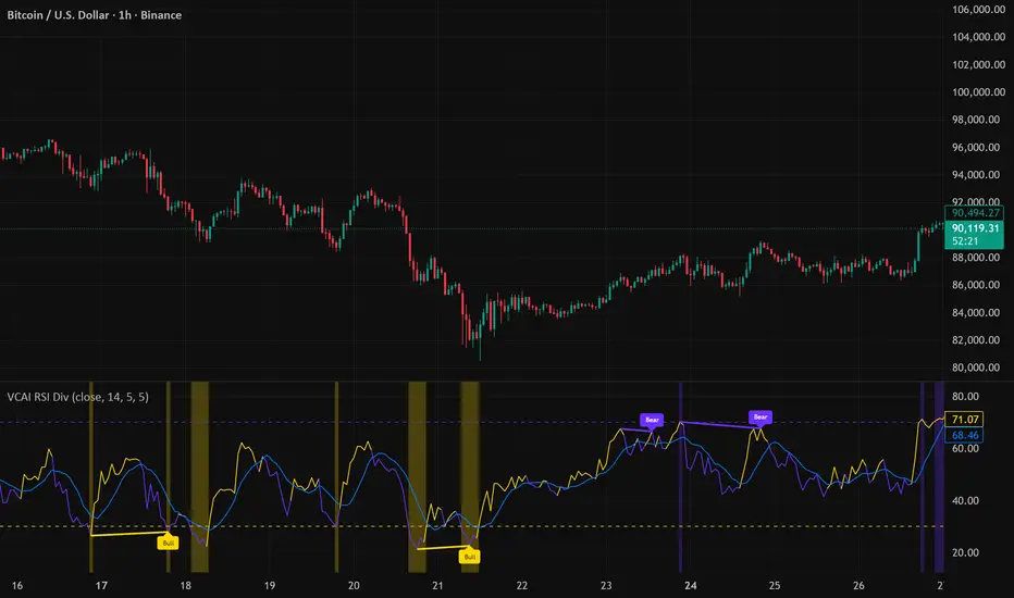
VCAI RSI Divergence +VCAI RSI Divergence+ is an RSI that shows trend, momentum, and divergence using V-CoresAI colour logic instead of a single white line.
What it shows:
Yellow RSI line → bullish momentum (RSI above its MA; buy-side pressure in control)
Purple RSI line → bearish momentum (RSI below its MA; sell-side pressure in control)
Thin blue line → fast RSI moving average that drives the colour flips
Dashed 70/30 lines → classic OB/OS zones
Background bands → soft purple in OB, soft yellow in OS to mark exhaustion areas
How to read it:
Yellow & rising → momentum shifting bullish; pullbacks into yellow OS band can be accumulation zones
Purple & falling → momentum shifting bearish; pushes into purple OB band can be distribution/sell zones
Hard colour flips (yellow ↔ purple) mark trend regime changes, not minor RSI noise
Divergence mode (on/off)
The divergence engine scans RSI and price pivot structure:
Bullish divergence (yellow) → price lower low + RSI higher low
Bearish divergence (purple) → price higher high + RSI lower high
Lines and tags appear only where a meaningful disagreement between price and RSI exists, giving early context for potential reversals or fade setups.
Together, the momentum colours + optional divergence mapping give a far clearer market read than a standard RSI, with zero clutter and no guesswork.
M-oscillator
Orca Trade PendulumMomentum oscillator with dual-EMA engine, ATR normalization, and Flip reversal signals. Candle coloring and dynamic histogram included.
Orca Trade Pendulum is a closed-source momentum and reversal detection oscillator designed to identify shifts in trend strength, momentum acceleration, and key turning points.
It combines a dual-EMA engine, ATR normalization, a dynamic pendulum-style histogram, and a Flip-Signal system that highlights moments when momentum changes direction after leaving overbought or oversold zones.
Key features:
• ORCA Dual-EMA Momentum Engine
• ATR-normalized oscillator for adaptive scaling
• Pendulum Histogram showing momentum acceleration and deceleration
• Flip Signals confirming momentum reversal after OB/OS exit
• Automatic candle coloring on flip confirmation
• Optional signal line for smooth trend interpretation
• Overbought and oversold levels with background highlighting
This is a protected-source script.
The code is hidden and cannot be viewed or copied.
The script is provided for testing and evaluation.

Estrategia Visual PRO: Momentum EditionIndicador con estrategia propia basado en cruce de emas editables son sombreado de tendencia del precio y niveles de soporte y resistencias donde el precio tiene reaccion, tambien cuenta con filtro de rsi donde colorea las velas segun la fuerza del rsi, colores editables y cuando el precio pierde fuerza
This indicator, with its own strategy based on editable EMA crossovers, features price trend shading and support and resistance levels where the price reacts. It also includes an RSI filter that colors the candles according to the strength of the RSI, with editable colors, and alerts you when the price loses strength.

RSI Pivot Breaks█ OVERVIEW
RSI Pivot Breaks is an RSI-based indicator that detects breakout events on oscillator-based pivot levels (RSI or MA RSI).
The tool automatically plots pivot levels, tracks their breakouts, highlights momentum shifts, and generates alerts for key events (pivot breaks and OB/OS crosses).
The indicator is designed primarily for momentum strategies — pivot breakouts often precede directional price moves, making RSI Pivot Breaks a powerful tool for identifying accelerations and changes in strength.
█ CONCEPTS
The indicator analyzes local RSI extremes and transforms them into dynamic support/resistance levels.
When RSI or MA RSI breaks the last pivot, it signals a shift in momentum balance, often leading to an impulse move.
Key concepts:
- pivot highs/lows detected on RSI or MA RSI,
- pivot lines extend forward until broken,
- pivot filters restrict pivot detection to specific RSI zones,
- OB/OS levels provide contextual momentum thresholds.
█ FEATURES
Pivot Detection & Breakouts
- Detection of pivot highs and lows on RSI or MA RSI.
- Pivot filters allow you to limit pivot detection to specific RSI ranges (e.g., only bullish pivots below 50 or bearish pivots above 50).
- Pivot lines update automatically after breakout.
Background highlights:
- green on pivot-high breakouts,
- red on pivot-low breakouts.
RSI & MA RSI
- Dynamic RSI colors based on momentum direction.
- Optional MA RSI line (SMA/EMA/RMA/WMA) usable as a smoother pivot source.
OB / OS Zones
- Fully adjustable overbought/oversold levels.
- Dedicated OB/OS colors.
- Optional gradient backgrounds.
Highlights
- Instant identification of moments when RSI breaks a key pivot level.
Alerts:
- pivot high breakouts.
- pivot low breakouts.
- OB crosses.
- OS crosses.
█ HOW TO USE
Add the indicator:
Indicators → RSI Pivot Breaks.
RSI Settings
- RSI Length – core RSI period.
- RSI MA Length & Type – MA RSI smoothing parameters.
Pivot Settings
- Pivot Left / Pivot Right – number of bars required to form a pivot and also the number of bars of delay before the pivot becomes confirmed.
(Higher values produce more reliable but slower pivots.)
Pivot Filters
- Minimum/maximum allowed RSI levels for pivot Highs and Lows.
- Examples:
- detect only pivot Highs at low RSI values.
- ignore pivots during extreme momentum.
- allow only mid-range pivot detection depending on strategy.
Visualization
- Toggles for RSI and MA RSI visibility.
- Optional gradients.
- Full color and transparency customization.
OB/OS Levels
- Adjustable thresholds depending on instrument volatility and strategy style.
█ SIGNAL INTERPRETATION
BUY
- RSI breaks the latest pivot high.
- RSI crosses upward out of OS.
- Context example: pivot lows forming a rising sequence.
SELL
- RSI breaks the latest pivot low.
- RSI drops downward from OB.
- Context example: pivot highs forming a declining sequence.
Trend / Momentum
- Pivot breakouts indicate acceleration or continuation of momentum.
- MA-based pivots provide smoother and more stable momentum structure.
█ APPLICATIONS
- Momentum Trading – pivot breaks as early acceleration signals.
- Scalping & Intraday – fast RSI pivots react quickly to short-term shifts.
- Swing Trading – smoother pivots using MA RSI for higher-timeframe structure.
- Divergence Detection – pivot behavior helps reveal divergence patterns, e.g.:
- RSI pivots rising while price is falling → potential early momentum reversal.
- Custom Filtering – pivot filters allow, for example:
- blocking bullish signals near OB.
- blocking bearish signals near OS.
- detecting pivots only above/below mid-range during strong trends,
depending entirely on strategy design.
█ NOTES
- Pivot detection includes natural delay equal to the Left/Right parameters.
- Pivot filters significantly change the character of signals, allowing fine-tuning of aggressiveness for any strategy.

VCAI MACD LiteVCAI MACD Lite is a clean, modern version of the classic MACD oscillator, rebuilt with selectable EMA/SMA types and a 2-tone histogram using VCAI’s visual style.
It keeps the indicator lightweight and easy to read while giving clearer momentum shifts through rising/falling histogram colour changes.
What it does
Calculates MACD using your choice of EMA or SMA
Plots signal line and histogram with 2-tone VCAI colours
Highlights changes in momentum strength as histogram bars rise or fade
Works on any market and timeframe
How to use it
Expanding yellow bars reflect strengthening upside momentum; dim yellow shows fading strength.
Darker and lighter VCAI purple tones show momentum behaviour below zero, helping you see when bearish pressure is increasing or weakening.
Part of the VCAI Lite Series — clean, minimal tools.

Institutional MF-Vol Compression Scanner v4.0 [BIG]═══════════════════════════════════════════════════════════════════════════════
BIG COMPRESSION SCANNER v4.0
═══════════════════════════════════════════════════════════════════════════════
OVERVIEW
The BIG Compression Scanner v4.0 is a proprietary volatility regime detection system designed for systematic Daily options deployment. This framework identifies pre-expansion volatility compression zones through multi-dimensional market structure analysis, combining institutional positioning patterns with hierarchical timeframe confirmation and options market structure to generate high-conviction directional signals for premium strategies.
The methodology synthesizes volatility dynamics, liquidity flow patterns, and cross-timeframe regime alignment into a probabilistic scoring system that isolates asymmetric risk-reward setups characteristic of compression-to-expansion transitions. The framework is calibrated specifically for 30-45 DTE options strategies where timing precision and volatility environment assessment are critical to edge generation.
═══════════════════════════════════════════════════════════════════════════════
CORE METHODOLOGY
═══════════════════════════════════════════════════════════════════════════════
• Proprietary Compression Detection
The system employs a multi-factor compression identification framework that monitors volatility regime transitions across price dispersion metrics and range contraction patterns. Unlike single-indicator squeeze systems, this methodology uses weighted ensemble logic to distinguish true pre-expansion compression from random consolidation noise.
Compression strength is quantified through a proprietary scoring algorithm (0-100%) that evaluates:
- Statistical volatility contraction relative to historical norms
- Price range compression within dynamic envelope systems
- Institutional volume signature analysis during low-volatility periods
- Cross-timeframe compression alignment (Daily/Weekly/Monthly hierarchy)
The framework filters compression events based on minimum strength thresholds and multi-bar confirmation to eliminate premature signals characteristic of retail squeeze indicators.
• Hierarchical Multi-Timeframe Architecture
The indicator integrates a three-tier temporal analysis structure where higher timeframes constrain and validate lower timeframe signals:
Strategic Layer (Monthly) – Establishes macro directional bias and identifies structural market positioning. This layer determines whether intermediate trends align with or counter dominant regime dynamics.
Structural Layer (Weekly) – Provides tactical context through key price levels, momentum assessment, and volatility regime confirmation. Weekly analysis filters signals that would occur in unfavorable proximity to structural inflection zones.
Execution Layer (Daily) – Generates precise entry timing through intraday regime shift detection, momentum confluence analysis, and institutional flow pattern recognition.
Each layer contributes weighted influence to the composite directional probability model, with recalibration logic that adjusts timeframe importance based on current market regime characteristics. The exact weighting algorithm is proprietary and adapts to volatility environment dynamics.
• Options Market Structure Integration
Version 4.0 incorporates options-specific market intelligence not available in standard technical analysis frameworks:
Volatility Environment Assessment – The system continuously monitors implied volatility regime characteristics through proprietary estimation models. These models identify whether current premium levels favor buying or selling strategies, adjusting signal generation accordingly.
Temporal Decay Awareness – Built-in expiration cycle logic ensures signals only trigger when sufficient time value remains for thesis development. The framework approximates days-to-expiration and applies minimum threshold filters to prevent entries in high theta decay regimes.
Greeks-Aware Targeting – Price targets are dynamically calibrated based on volatility expansion expectations and estimated leverage characteristics. Target multipliers adjust to current options market structure rather than using fixed risk-reward ratios.
Premium Environment Classification – Signals are enhanced with real-time assessment of whether current volatility levels favor long premium, short premium, or spread strategies based on historical percentile analysis.
• Probabilistic Directional Scoring System
Rather than binary bullish/bearish classification, the framework generates probability-weighted directional bias through a proprietary multi-factor model. This model synthesizes trend alignment metrics, momentum characteristics, structural positioning, and institutional flow signatures into normalized probability distributions.
The scoring system evaluates dozens of market structure variables across multiple timeframes, applies regime-dependent weighting, and produces directional probabilities that reflect actual edge rather than arbitrary technical indicator thresholds. Signal generation occurs only when directional probability exceeds user-defined conviction thresholds (55-65% depending on sensitivity setting).
This probabilistic approach allows traders to calibrate position sizing and strategy selection (outright vs. spreads) to the strength of directional conviction rather than treating all signals as equal weight.
• Institutional Flow Detection
The framework monitors volume and price interaction patterns characteristic of institutional accumulation or distribution during compression phases. This analysis identifies whether compression zones contain building directional positions (high probability of sustained move post-breakout) versus thin, choppy consolidation (high false breakout risk).
Flow detection employs proprietary algorithms that distinguish genuine institutional activity from retail volume spikes, providing critical context for signal validation.
═══════════════════════════════════════════════════════════════════════════════
SIGNAL ARCHITECTURE
═══════════════════════════════════════════════════════════════════════════════
Call Option Signals trigger when compression strength, directional probability, timeframe alignment, options market structure, and institutional flow patterns simultaneously satisfy proprietary threshold criteria. Signals are filtered against weekly structural levels to avoid low-probability entries near major resistance zones.
Put Option Signals follow equivalent logic with inverse directional parameters, ensuring symmetrical framework application across bull and bear setups.
All signals include:
- Directional conviction probability (percentage)
- Current volatility environment assessment (IV Rank proxy)
- Dynamic price target based on expansion expectations
- Multi-timeframe alignment status
Signal cooldown logic prevents excessive signal generation during extended consolidation periods, maintaining signal quality over quantity.
═══════════════════════════════════════════════════════════════════════════════
VISUAL INTELLIGENCE
═══════════════════════════════════════════════════════════════════════════════
Real-Time Multi-Timeframe Dashboard
The top-right panel provides continuous visibility into:
- Trend alignment across Daily/Weekly/Monthly timeframes
- Current compression status at each temporal layer
- Momentum regime characteristics (RSI values)
- Options environment assessment (IV Rank, optimal strategy)
- Composite signal readiness (compression strength percentage)
This dashboard enables rapid regime assessment without manual multi-timeframe chart analysis.
Chart Integration
Visual overlays include:
- Volatility envelope systems (dynamic bands)
- Weekly structural price levels (pivot, resistance, support)
- Compression zone highlighting (background shading)
- Active squeeze indicators (Daily and Weekly differentiation)
Signal Labels
When setups trigger, comprehensive labels display:
📈 CALL OPTION
Prob: XX%
IV Rank: XX%
Target: $XXX.XX
Labels provide all critical execution information without requiring dashboard consultation.
═══════════════════════════════════════════════════════════════════════════════
KEY CAPABILITIES
═══════════════════════════════════════════════════════════════════════════════
- Proprietary multi-factor compression detection with adaptive thresholds
- Hierarchical multi-timeframe confirmation (Daily/Weekly/Monthly)
- Options-specific filters (IV regime, DTE requirements, Greeks awareness)
- Probabilistic directional scoring (0-100% conviction levels)
- Institutional flow pattern recognition during compression
- Weekly structural level integration with proximity filters
- Dynamic target calibration based on volatility expansion expectations
- Real-time multi-timeframe regime dashboard
- Customizable sensitivity and threshold parameters
- Non-repainting signal architecture (bar close confirmation)
- Comprehensive alert system for proactive monitoring
═══════════════════════════════════════════════════════════════════════════════
APPLICATION GUIDELINES
═══════════════════════════════════════════════════════════════════════════════
1. Timeframe Selection
Apply to Daily (D1) charts only. Framework calibration is timeframe-specific; other intervals produce suboptimal results.
2. Options Mode Activation
Enable Options Trading Mode for premium strategy optimization. This activates IV filtering, DTE thresholds, and Greeks-aware targeting.
3. Strategy Calibration
- Premium Buying: Set IV threshold to 50th percentile, DTE minimum 30+ days, target multiplier 2.5-3.0×
- Premium Selling: Set IV threshold to 70th+ percentile, DTE minimum 20-30 days, target multiplier 1.5-2.0×
4. MTF Dashboard Monitoring
Verify multi-timeframe alignment before execution:
- Ideal setup: Daily + Weekly compression both active
- Confirm trend alignment across timeframes
- Check IV Rank for premium environment assessment
- Wait for "READY" status (green) indicating threshold satisfaction
5. Signal Execution
When labels appear:
- Review directional probability (target >65% for high conviction)
- Assess IV environment (low IV favors buying, high IV favors selling)
- Use price target for strike selection and profit objectives
- Consider 30-45 DTE options for thesis development time
6. Risk Management
- Position size: 2-5% options capital per signal
- Stop loss: Exit if compression breaks opposite direction without follow-through
- Time stop: Reassess if position stagnant after 5-7 days
- Profit taking: Scale out at provided targets or weekly pivot levels
7. Sensitivity Adjustment
- High (55%): More signals, lower conviction, diversified approach
- Medium (60%): Balanced, default setting (2-4 signals/month typical)
- Low (65%): Fewer signals, higher conviction, concentrated positions
═══════════════════════════════════════════════════════════════════════════════
FRAMEWORK LIMITATIONS
═══════════════════════════════════════════════════════════════════════════════
- Optimized exclusively for Daily timeframe analysis
- Compression development requires patience (2-4 weeks typical)
- IV metrics are proprietary proxies, not direct exchange data
- Greeks estimations approximate actual options contract characteristics
- DTE calculations simplified vs. precise monthly expiration dates
- Multi-timeframe filtering reduces but cannot eliminate false breakouts
- Requires liquid options markets (tight spreads, adequate open interest)
- Not designed for earnings-driven volatility events (IV crush risk)
- Framework identifies timing, not specific strike or expiration selection
═══════════════════════════════════════════════════════════════════════════════
TECHNICAL SPECIFICATIONS
═══════════════════════════════════════════════════════════════════════════════
- Pine Script v5 architecture
- Non-repainting signal confirmation (bar close validation)
- Multi-security data integration (Weekly/Monthly via request.security)
- Real-time multi-timeframe analysis dashboard
- 4 alert conditions (Call/Put options, directional generic)
- Fully customizable parameters (compression, scoring, filters, visuals)
- Professional-grade visual hierarchy and information density
═══════════════════════════════════════════════════════════════════════════════
PROFESSIONAL CONTEXT
═══════════════════════════════════════════════════════════════════════════════
This framework is designed for systematic options traders with working knowledge of:
- Volatility regime dynamics and expansion/contraction cycles
- Options Greeks and their impact on P&L across various market conditions
- Implied Volatility Rank interpretation and premium pricing assessment
- Multi-timeframe analysis methodology and trend hierarchy
- Risk-adjusted position sizing and portfolio construction principles
The system identifies when market structure favors options deployment but does not prescribe how to construct positions. Strike selection, expiration choice, spread architecture, and position sizing require independent trader judgment based on account parameters and risk tolerance.
Optimal deployment combines this framework with:
- Options analytics platform (actual IV, Greeks, probability calculations)
- Earnings calendar awareness (pre-earnings IV inflation vs. post-earnings crush)
- Broader market regime context (VIX, correlation, sector rotation)
- Portfolio-level risk management (concentration limits, correlation analysis)
═══════════════════════════════════════════════════════════════════════════════
Proprietary compression-to-expansion framework for systematic Daily options deployment. Methodology incorporates multi-dimensional volatility analysis, hierarchical timeframe confirmation, and options market structure intelligence.

NHNL Breadth Scanner [BIG]═══════════════════════════════════════════════════════════════════════════════
NVENTURES NHNL BREADTH SYSTEM v2.0
═══════════════════════════════════════════════════════════════════════════════
OVERVIEW
The NVentures NHNL Breadth System is an institutional-grade market breadth analysis framework designed for equity traders, portfolio managers, and market technicians who require comprehensive internal market structure visibility beyond price action alone. This system integrates New Highs - New Lows (NHNL) data across multiple exchanges with participation breadth metrics to identify market regime shifts, thrust conditions, divergences, and rotation dynamics between large-cap and small-cap equities.
Version 2.0 introduces the Participation Breadth Module , which monitors the percentage of stocks above their 50-day moving averages across S&P 500, Russell 2000, and NASDAQ 100 indices. This extension enables detection of Risk-On/Risk-Off rotations and narrow rally conditions—critical information for portfolio construction, sector allocation, and tactical hedging decisions.
The framework combines:
- Multi-exchange NHNL aggregation – NYSE, NASDAQ, AMEX breadth data integration
- McClellan Oscillator – Exponential moving average difference for trend momentum
- Thrust detection – Extreme breadth expansion/contraction identification
- Divergence analysis – Price vs. breadth non-confirmation patterns
- Participation breadth – Large-cap vs. small-cap rotation detection
- Composite signal scoring – Multi-factor quantitative breadth assessment
═══════════════════════════════════════════════════════════════════════════════
CORE METHODOLOGY
═══════════════════════════════════════════════════════════════════════════════
• NHNL Data Aggregation
The system retrieves daily New Highs and New Lows from three major U.S. exchanges:
- NYSE – INDEX:HIGN (New Highs), INDEX:LOWN (New Lows)
- NASDAQ – INDEX:HIGQ (New Highs), INDEX:LOWQ (New Lows)
- AMEX – INDEX:HIGA (New Highs), INDEX:LOWA (New Lows)
Users can toggle exchanges on/off to isolate specific market segments. All three exchanges are enabled by default for comprehensive market-wide breadth measurement.
Core Calculations :
- NHNL Raw = Total New Highs - Total New Lows
- NHNL % = (NHNL Raw / Total Issues) × 100
- NH/NL Ratio = New Highs / New Lows
These metrics quantify the internal strength or weakness of market advances/declines independent of price index levels.
• McClellan Oscillator
The McClellan Oscillator applies exponential moving average (EMA) logic to NHNL data:
Formula: McClellan Osc = EMA(NHNL, Fast) - EMA(NHNL, Slow)
Default parameters: Fast = 19, Slow = 39
Interpretation :
- Positive values = Breadth momentum favors bulls (more issues making new highs)
- Negative values = Breadth momentum favors bears (more issues making new lows)
- Zero-line crosses = Regime change signals (bullish above, bearish below)
- Extreme readings (>±100) = Overbought/oversold breadth conditions
The McClellan Oscillator is a standard institutional breadth tool used by market technicians since the 1960s. It smooths daily NHNL volatility while maintaining responsiveness to trend changes.
• Thrust Detection
Thrust conditions identify extreme breadth expansion or contraction that historically precedes sustained directional moves:
Bullish Thrust :
- NHNL % > Threshold (default +40%)
- Sustained for Confirmation Bars (default 2 bars)
- Context : Extreme positive breadth expansion. Historically associated with major rally initiations or continuation thrusts.
Bearish Thrust :
- NHNL % < -Threshold (default -40%)
- Sustained for Confirmation Bars (default 2 bars)
- Context : Extreme negative breadth contraction. Historically associated with panic selling, capitulation events, or major downtrend acceleration.
Thrust conditions are the highest-priority signals in the framework and override other conflicting indicators.
• Divergence Detection
The system identifies non-confirmation patterns between price action and breadth:
Bullish Divergence :
- Price makes lower low
- NHNL % makes higher low
- Context : Selling pressure exhausting despite lower prices. Potential reversal signal as fewer stocks participate in decline.
Bearish Divergence :
- Price makes higher high
- NHNL % makes lower high
- Context : Rally losing internal momentum despite higher prices. Potential reversal signal as fewer stocks participate in advance.
Divergences use pivot detection with configurable lookback periods (default 50 bars) and pivot strength (default 5 bars). Visual divergence lines are drawn directly on the price chart when detected.
• Participation Breadth Module (NEW in v2.0)
This module monitors the percentage of stocks trading above their 50-day moving average across three major indices:
- S&P 500 – INDEX:S5FI (Large-cap participation)
- Russell 2000 – INDEX:R2FI (Small-cap participation)
- NASDAQ 100 – INDEX:NDFI (Tech-cap participation)
Rotation Spread Calculation :
Rotation Spread = Russell 2000 % Above 50D - S&P 500 % Above 50D
Interpretation :
- Positive Spread (>+10%) = Risk-On Rotation
Small caps outperforming large caps. Broad market participation. Risk appetite expanding.
- Negative Spread (<-10%) = Risk-Off Rotation
Large caps outperforming small caps. Narrow rally / defensive positioning. Flight to quality or concentration risk.
- Neutral (-10% to +10%) = Balanced market, no clear rotation
This spread identifies critical regime changes between broad market participation (healthy) and narrow leadership (fragile). Risk-On rotations typically occur during economic expansion phases; Risk-Off rotations occur during uncertainty, recession fears, or late-cycle conditions.
• Composite Signal Score
The framework generates a quantitative breadth score (-100 to +100) by weighting five components:
1. Thrust Score (±40 points) – Active thrust condition
2. Trend Score (±30 points) – McClellan Oscillator above/below zero
3. Momentum Score (±20 points) – NHNL % magnitude
4. Ratio Score (±10 points) – NH/NL Ratio extremes
5. Participation Score (±15 points) – Risk-On/Risk-Off regime + participation health
The composite score is smoothed (EMA 5) and classified into five breadth states:
- +50 to +100 = Strong Bull
- +20 to +50 = Bullish
- -20 to +20 = Neutral
- -50 to -20 = Bearish
- -100 to -50 = Strong Bear
═══════════════════════════════════════════════════════════════════════════════
SIGNAL HIERARCHY & PRIORITY
═══════════════════════════════════════════════════════════════════════════════
The indicator generates multiple signal types with distinct priority levels:
Priority 1: Thrust Signals (Highest conviction)
- Green triangle below bar = Bullish Thrust (40%+ breadth expansion)
- Red triangle above bar = Bearish Thrust (40%+ breadth contraction)
- Chart background highlighted in green/red during active thrust
Priority 2: Rotation Signals (Regime identification)
- Cyan diamond below bar = Risk-On Rotation (small caps outperforming)
- Orange diamond above bar = Risk-Off Rotation (large caps outperforming)
- Chart background highlighted in cyan/orange during active rotation
Priority 3: Divergence Signals (Reversal warnings)
- Green label below bar = Bullish Divergence (price/breadth non-confirmation)
- Red label above bar = Bearish Divergence (price/breadth non-confirmation)
- Dashed lines connect divergence pivot points on price chart
Priority 4: Zero-Line Cross (Trend changes)
- Small circle below bar = McClellan crossing above zero (breadth turning positive)
- Small circle above bar = McClellan crossing below zero (breadth turning negative)
═══════════════════════════════════════════════════════════════════════════════
VISUAL COMPONENTS
═══════════════════════════════════════════════════════════════════════════════
• Comprehensive Information Panel
The top-right dashboard (position customizable) displays:
Section 1: Raw NHNL Data
- Total New Highs (green)
- Total New Lows (red)
- Exchange breakdown (NYSE, NASDAQ, AMEX) with individual deltas
Section 2: Core Metrics
- NHNL % with visual indicator (🔥 for thrusts, arrows for direction)
- NH/NL Ratio with strength bars
- McClellan Oscillator with directional arrows
Section 3: Participation Breadth (NEW)
- S&P 500 % above 50D MA with trend arrow
- Russell 2000 % above 50D MA with trend arrow
- NASDAQ 100 % above 50D MA with trend arrow
- Rotation Spread with regime icon (🚀 Risk-On, 🛡️ Risk-Off)
Section 4: Composite Assessment
- Signal Score (-100 to +100) with visual strength bars
- Market Status (large text): BULLISH THRUST, BEARISH THRUST, RISK-ON ROTATION, RISK-OFF ROTATION, or breadth state classification
• Chart Overlays
- Background color-coding for active regimes (thrust, rotation, extreme readings)
- Signal markers (triangles, diamonds, circles, labels) at key inflection points
- Divergence lines connecting pivot highs/lows on price chart
═══════════════════════════════════════════════════════════════════════════════
KEY FEATURES
═══════════════════════════════════════════════════════════════════════════════
- Multi-exchange breadth aggregation – NYSE, NASDAQ, AMEX with individual on/off toggles
- Institutional McClellan Oscillator – Standard market breadth momentum tool
- Automated thrust detection – Identifies extreme breadth conditions with confirmation logic
- Price-breadth divergence scanning – Non-confirmation pattern detection with visual lines
- Participation breadth integration – Risk-On/Risk-Off rotation detection via large-cap vs. small-cap analysis
- Composite signal scoring – Quantitative multi-factor breadth assessment
- No repainting – All signals confirm on bar close
- Comprehensive alerting – 12+ alert conditions for thrust, divergence, rotation, and confluence events
- Fully customizable parameters – EMA periods, thresholds, lookbacks, visual settings
- Professional dashboard – Real-time metrics with color-coded status indicators
═══════════════════════════════════════════════════════════════════════════════
HOW TO USE
═══════════════════════════════════════════════════════════════════════════════
1. Apply to any chart – The indicator pulls multi-security data; chart symbol does not matter (commonly applied to SPY, SPX, or QQQ for reference)
2. Monitor the dashboard :
• Focus on Market Status (bottom row) for current regime
• Check NHNL % and McClellan for breadth direction and momentum
• Watch Rotation Spread for large-cap vs. small-cap dynamics
• Review Signal Score for composite breadth strength
3. Interpret thrust signals (highest priority):
• Bullish Thrust → Major rally initiation or continuation likely. Consider adding long exposure or reducing hedges.
• Bearish Thrust → Major decline or capitulation event likely. Consider reducing exposure or adding hedges.
• Historical context: Thrust signals are rare (2-5 per year) but highly reliable for significant market moves.
4. Interpret rotation signals (regime identification):
• Risk-On Rotation → Broad market participation. Small caps outperforming. Healthy advance. Favor cyclical sectors, higher beta names.
• Risk-Off Rotation → Narrow rally or defensive positioning. Large caps outperforming. Caution—market leadership concentrating. Favor quality, defensives.
5. Interpret divergence signals (reversal warnings):
• Bullish Divergence → Selling exhaustion. Potential bottom formation. Wait for confirmation (zero-line cross, thrust) before aggressive positioning.
• Bearish Divergence → Rally losing momentum. Potential top formation. Consider profit-taking or hedging.
6. Combine signals for maximum conviction :
• Bull Confluence : Bullish Thrust + Risk-On Rotation + Positive McClellan = Maximum bullish alignment
• Bear Confluence : Bearish Thrust + Risk-Off Rotation + Negative McClellan = Maximum bearish alignment
• Alert system specifically flags these high-conviction confluences
7. Configure parameters for your style :
• Thrust Threshold : Default 40% catches major moves. Increase to 50%+ for extreme-only signals.
• Rotation Threshold : Default 10% spread. Tighten to 7.5% for earlier rotation detection.
• Divergence Lookback : Default 50 bars. Extend to 100+ for longer-term divergences.
8. Use alerts for proactive monitoring :
• Set TradingView alerts for Thrust, Rotation, Divergence, and Confluence conditions
• Receive notifications when critical breadth regime changes occur
═══════════════════════════════════════════════════════════════════════════════
LIMITATIONS
═══════════════════════════════════════════════════════════════════════════════
- U.S. equity markets only – NHNL data limited to NYSE, NASDAQ, AMEX. Does not cover international markets or other asset classes.
- Daily timeframe only – NHNL data is reported daily. Intraday trading requires alternative breadth measures.
- Lagging in fast reversals – McClellan Oscillator and participation metrics use EMAs, introducing lag during rapid regime shifts. Thrust signals respond faster but require extreme conditions.
- Equal-weighting assumption – All stocks within NHNL counts are equally weighted. Large-cap-dominated rallies (e.g., FANG-led advances) may show strong price performance despite mediocre breadth.
- False positives in sideways markets – Divergence signals can produce false positives during extended consolidation phases. Require confirmation from thrust or rotation signals.
- Participation data quality – S5FI, R2FI, NDFI data from TradingView may have occasional gaps or delays. Indicator includes data validation logic and falls back gracefully when data unavailable.
═══════════════════════════════════════════════════════════════════════════════
TECHNICAL SPECIFICATIONS
═══════════════════════════════════════════════════════════════════════════════
- Pine Script v5
- Non-repainting (signals confirmed on bar close)
- Multi-security data feeds (6 NHNL tickers + 3 participation tickers)
- Maximum 500 lines supported (divergence line drawing)
- Real-time dashboard table with 20+ rows
- 12+ alert conditions (thrust, divergence, rotation, ratio extremes, confluence)
- Fully customizable colors, thresholds, and visual elements
═══════════════════════════════════════════════════════════════════════════════
NOTES
═══════════════════════════════════════════════════════════════════════════════
This indicator is designed for experienced equity traders, portfolio managers, and market technicians familiar with:
- Market breadth analysis and internal market structure
- McClellan Oscillator interpretation
- New High - New Low dynamics and their correlation with market cycles
- Large-cap vs. small-cap rotation patterns
- Risk-On/Risk-Off regime identification
The framework provides objective breadth signals but does not account for:
- Fundamental catalysts (earnings, economic data, Fed policy)
- Sector-specific dynamics (may show broad weakness while certain sectors thrive)
- International market correlations
- Volatility regime changes (VIX dynamics)
Best used in combination with:
- Price action analysis (support/resistance, chart patterns)
- Volume analysis (accumulation/distribution)
- Volatility indicators (VIX, put/call ratios)
- Sentiment indicators (survey data, positioning)
Market breadth is a leading indicator of internal market health. Divergences between price and breadth often precede major reversals by weeks or months.
═══════════════════════════════════════════════════════════════════════════════
Developed for institutional market breadth analysis based on New Highs - New Lows methodology with extended participation breadth integration.

Majors FX-REER/NEER Suite [BIG]═══════════════════════════════════════════════════════════════════════════════
BIG MAJORS FX-REER/NEER SUITE
═══════════════════════════════════════════════════════════════════════════════
OVERVIEW
The BIG Majors FX-REER/NEER Suite is a multi-currency valuation framework designed for institutional FX traders, macro strategists, and systematic currency allocators. This indicator calculates Real Effective Exchange Rates (REER) and Nominal Effective Exchange Rates (NEER) for the seven major currency pairs (G7 FX), integrating macroeconomic fundamentals (CPI inflation differentials) with technical trend analysis to identify structural currency misvaluations and mean-reversion opportunities.
Unlike standard FX indicators that only analyze bilateral price action, this suite constructs trade-weighted basket indices that measure each currency's strength against a portfolio of its major trading partners, adjusted for inflation differentials. This approach mirrors central bank and sovereign wealth fund methodologies for assessing equilibrium exchange rate levels.
The framework combines:
- Fundamental valuation metrics – REER/NEER indices with Z-score normalization
- Technical trend filters – Ichimoku Cloud and Aroon oscillator confluence
- Signal classification system – Long/Short/Watch/Conflict regime identification
- Quantitative confidence scoring – 0-100% signal reliability weighting
═══════════════════════════════════════════════════════════════════════════════
CORE METHODOLOGY
═══════════════════════════════════════════════════════════════════════════════
• NEER Calculation (Nominal Effective Exchange Rate)
The NEER measures a currency's value against a trade-weighted basket of its seven major trading partners, geometrically averaged in log-space to ensure symmetry:
1. All seven G7 FX pairs are normalized to USD-pivot (A/USD format)
2. Each currency's log-normalized rate is compared to the arithmetic mean of the other six
3. Formula: NEER_i = (8/7) × log(CCY_i/USD) - mean(log(CCY_others/USD))
This construction ensures that:
- A rising NEER indicates currency appreciation against the basket
- The methodology is symmetric and avoids base-currency bias
- Changes reflect multilateral competitive dynamics, not just bilateral moves
• REER Calculation (Real Effective Exchange Rate)
The REER adjusts the NEER for inflation differentials using Consumer Price Index (CPI) data:
Formula: REER_i = NEER_i + log(CPI_i) - mean(log(CPI_others))
By incorporating CPI differentials, the REER provides a purchasing-power-parity-adjusted valuation metric that accounts for relative inflation rates. This is the institutional standard for assessing fundamental currency equilibrium levels.
Data Sources :
- FX rates: TradingView composite feed (FX:), OANDA, FXCM, FOREXCOM
- CPI data: ECONOMICS namespace (monthly frequency, official statistical releases)
- Supported currencies: USD, EUR, JPY, GBP, CHF, AUD, CAD, NZD
• Valuation Bias Detection
Each currency pair is classified as overvalued (bias = -1, "Short") or undervalued (bias = +1, "Long") based on two independent criteria:
1. Percentage Band Deviation – Relative Index distance from 100 baseline
• Overvalued: Index > 100 × (1 + deviation%), default +5%
• Undervalued: Index < 100 × (1 - deviation%), default -5%
2. Z-Score Threshold – Statistical extremes in rolling lookback window
• Overvalued: Z-Score > +1.5 (default)
• Undervalued: Z-Score < -1.5 (default)
Either condition triggers a bias classification. This dual-filter approach captures both absolute deviations and relative extremes within recent historical context.
• Trend Confirmation (Ichimoku + Aroon)
To avoid counter-trend entries in strong momentum regimes, the suite integrates two independent trend filters:
Ichimoku Cloud
- Bull: Price > Cloud AND Conversion > Base Line
- Bear: Price < Cloud AND Conversion < Base Line
- Parameters: Conv(9), Base(26), Span B(52), Displacement(26)
Aroon Oscillator
- Bull: Aroon Up > 70 AND Aroon Down < 30
- Bear: Aroon Down > 70 AND Aroon Up < 30
- Default lookback: 25 periods
Trend is confirmed only when both indicators agree (Ichimoku + Aroon ≥ +1 for bull, ≤ -1 for bear).
• Setup Classification Logic
The framework combines Bias (fundamental valuation) with Trend (technical momentum) to generate four distinct setup types:
- Long↗︎ (Setup = 1) – Undervalued + Bullish Trend
Context : Mean reversion opportunity with momentum confirmation. Currency trading at fundamental discount while technical trend supports upside.
- Short↘︎ (Setup = -1) – Overvalued + Bearish Trend
Context : Mean reversion opportunity with momentum confirmation. Currency trading at fundamental premium while technical trend supports downside.
- Watch (Setup = 2) – Valuation bias present, but no clear trend
Context : Fundamental mispricing without directional conviction. Monitor for trend emergence before entering.
- Conflict (Setup = 3) – Bias and trend pointing opposite directions
Context : Overvalued currency in uptrend OR undervalued currency in downtrend. Avoid—either trend continuation or valuation mean reversion, but unclear which dominates.
• Confidence Score (0-100%)
Each setup receives a quantitative confidence weighting based on three factors:
1. Band Distance (40%) – How far the Relative Index deviates from 100 baseline
2. Z-Score Magnitude (40%) – Statistical extremeness within lookback window
3. Trend Confluence (20%) – Agreement between Ichimoku and Aroon signals
Score interpretation:
- 70-100% = High confidence (both valuation and trend extremes aligned)
- 40-69% = Moderate confidence (one factor strong, others weak)
- 0-39% = Low confidence (marginal signals, questionable reliability)
═══════════════════════════════════════════════════════════════════════════════
VISUAL COMPONENTS
═══════════════════════════════════════════════════════════════════════════════
• Dashboard Table (Top-Right)
Displays real-time valuation metrics for all seven major pairs:
Column 1: Pair – Currency pair identifier
Column 2: RelIdx – Relative Index (100 = baseline at first valid bar)
Column 3: Z – Z-Score vs. rolling lookback window
Column 4: Bias – Long/Short/Neutral valuation classification
Column 5: Trend – ↑/↓/– trend direction (Ichimoku + Aroon)
Column 6: Setup – Long↗︎/Short↘︎/Watch/Conflict (color-coded)
Column 7: Conf – Confidence score 0-100% (color-coded)
Column 8: Quelle – REER (inflation-adjusted) or NEER (nominal only)
Color coding :
- Green = Long↗︎ setup
- Red = Short↘︎ setup
- Orange = Watch (no trend)
- Purple = Conflict (bias/trend divergence)
• Optional Chart Plot
Select any of the seven pairs to plot its Relative Index on the chart with:
- Baseline at 100 (horizontal gray line)
- +Band at 100 × (1 + deviation%), dashed red
- -Band at 100 × (1 - deviation%), dashed green
- Aqua line tracking the selected pair's Relative Index evolution
• Signal Labels
When a pair transitions into Long↗︎ or Short↘︎ setup:
- Green label below bar = Long↗︎ entry signal
- Red label above bar = Short↘︎ entry signal
- Positioned using ATR offset for visibility
═══════════════════════════════════════════════════════════════════════════════
KEY FEATURES
═══════════════════════════════════════════════════════════════════════════════
- Institutional valuation methodology – REER/NEER framework used by central banks and sovereign wealth funds
- Macro-fundamental integration – CPI inflation differentials adjust for purchasing power parity
- Multi-timeframe flexibility – Daily (D), Weekly (W), Monthly (M) resolution options
- Seven simultaneous pairs – Monitors all G7 FX majors in single unified dashboard
- No repainting – All signals confirm on bar close
- Automated alerts – TradingView notifications when setups transition (Long/Short triggers)
- Confidence weighting – Quantitative scoring allows position sizing calibration
- Fallback logic – Automatically switches to NEER if CPI data incomplete
═══════════════════════════════════════════════════════════════════════════════
HOW TO USE
═══════════════════════════════════════════════════════════════════════════════
1. Apply to any chart – The indicator pulls multi-security data; chart symbol does not matter (commonly applied to SPY or DXY for reference)
2. Select data feed – Default FX: (TradingView composite) is recommended; alternatives: OANDA, FXCM, FOREXCOM
3. Choose timeframe :
• Daily (D) = Swing trading, medium-term mean reversion (2-8 week horizons)
• Weekly (W) = Position trading, macro regime shifts (1-6 month horizons)
• Monthly (M) = Strategic allocation, long-term equilibrium analysis (6-24 month horizons)
4. Configure parameters :
• Z-Score Lookback : Default 252 (one trading year on Daily); adjust for timeframe (52 for Weekly, 36 for Monthly)
• Deviation Band : Default ±5%; tighten to ±3% for more signals, widen to ±7% for higher conviction
• Z-Threshold : Default ±1.5; increase to ±2.0 for extreme-only signals
5. Monitor dashboard table :
• Focus on pairs showing Long↗︎ or Short↘︎ setups with Conf ≥ 70%
• Watch for Watch setups transitioning to directional signals
• Avoid Conflict setups unless you have strong macro conviction
6. Execute mean-reversion trades :
• Long↗︎ = Buy undervalued currency (e.g., EURUSD Long if EUR undervalued)
• Short↘︎ = Sell overvalued currency (e.g., USDJPY Short if JPY overvalued)
• Target: Mean reversion toward 100 baseline or opposite band
7. Position sizing by confidence :
• High confidence (70-100%) → Standard position size
• Moderate confidence (40-69%) → Reduce size by 50%
• Low confidence (<40%) → Avoid or use minimal pilot size
8. Risk management :
• Stop loss: Place beyond recent swing high/low or 1.5× ATR
• Take profit: Opposite valuation band or 100 baseline
• Time stop: Exit if setup reverses (Long→Neutral→Short or vice versa)
═══════════════════════════════════════════════════════════════════════════════
LIMITATIONS
═══════════════════════════════════════════════════════════════════════════════
- CPI data lag – Consumer Price Index releases are monthly and report with 2-4 week delay. REER calculations may lag real-time inflation dynamics.
- Structural shifts ignored – The baseline (100) is set at first valid bar. Long-term structural appreciation/depreciation (e.g., 20-year USD bull market) is not accounted for. Suitable for cyclical mean reversion, not secular trend analysis.
- Equal-weighting assumption – All seven currencies are equally weighted in basket construction. Actual trade-weighted indices use GDP or trade volume weights, which this framework simplifies.
- No emerging market currencies – Limited to G7 majors (USD, EUR, JPY, GBP, CHF, AUD, CAD, NZD). Does not cover EM FX (e.g., CNY, BRL, MXN).
- Technical filter limitations – Ichimoku and Aroon are lagging indicators. In fast-moving markets (e.g., central bank interventions, geopolitical shocks), trend signals may arrive late.
- Mean reversion assumption – The framework assumes currencies revert to equilibrium. During regime changes (e.g., monetary policy divergence, crisis flows), deviations can persist or expand before eventual reversal.
═══════════════════════════════════════════════════════════════════════════════
TECHNICAL SPECIFICATIONS
═══════════════════════════════════════════════════════════════════════════════
- Pine Script v6
- Non-repainting (signals confirmed on bar close)
- Multi-security data feeds (7 FX pairs + 8 CPI series)
- Automated alert system (transitions to Long↗︎/Short↘︎)
- Real-time dashboard table (8 columns × 8 rows)
- Maximum 500 labels supported (100 per pair direction)
- Fallback logic: NEER used if CPI data unavailable
═══════════════════════════════════════════════════════════════════════════════
NOTES
═══════════════════════════════════════════════════════════════════════════════
This indicator is designed for experienced FX traders, macro strategists, and portfolio managers familiar with:
- Real and nominal effective exchange rate concepts
- Purchasing power parity theory and inflation differentials
- Multi-currency portfolio construction and basket hedging
- Carry trade and convergence strategies
- Central bank policy impacts on FX equilibrium levels
The framework provides objective valuation signals but does not account for:
- Interest rate differentials (carry)
- Capital flow dynamics (risk-on/risk-off)
- Central bank intervention zones
- Geopolitical risk premiums
Always combine REER/NEER valuation analysis with macro event calendars, positioning data (CFTC COT reports), and fundamental policy divergence assessments.
═══════════════════════════════════════════════════════════════════════════════
Developed for institutional FX valuation analysis based on central bank REER/NEER methodologies.

RSI Multi Levels kiawosch [TradingFinder] 7-14-42 Consolidation🔵 Introduction
The Relative Strength Index or RSI is a tool used to measure the speed and intensity of price movement, oscillating between zero and one hundred. It is commonly applied to identify strength or weakness in market momentum across different time intervals. Despite its simple formula and wide usage, the behavior of RSI within specific ranges often provides more precise information than traditional overbought and oversold levels.
The Multi RSI layout displays three RSI values with periods 7, 14 and 42. The seven period RSI plays the primary role in short term analysis. When this value enters predefined ranges, it shows highly consistent and interpretable behavior that can signal trend continuation, corrections or the start of a range structure. The other two values, RSI 14 and RSI 42, help reveal higher timeframe momentum and provide context for the depth and quality of price movement.
Three potential zones are defined, each representing a behavioral range. The position zones forms the basis for signal interpretation :
High Potential : 78 to 85 & 22 to 15
Mid Potential : 70 to 78 & 30 to 22
Low Potential : 58 to 62 & 42 to 38
These zones highlight areas where RSI reacts in specific ways to price movement. Entering the High Potential range usually aligns with new highs or lows in price and often precedes continuation after a correction. In contrast, reactions inside the Mid Potential range frequently appear during clean ranges or channel structures. This approach focuses on momentum quality and structural behavior rather than classic overbought and oversold thresholds.
In summary, the logic behind the signals follows three principles :
Trend continuation, When RSI 7 enters the High Potential zone and price prints a new high or low, continuation after a correction becomes the most likely outcome.
Reversal or slowdown, When RSI exits the High Potential zone while price is reaching a previous high or low, the probability of a short term reversal increases.
Range behavior, In clean ranges or channel structures, RSI 7 typically reacts inside the Mid Potential zone and produces consistent swing responses.
🔵 How to Use
This method is based on observing the repeating behavior of RSI within momentum zones and identifying moments when price continues after a shallow correction or, conversely, when signs of slowing and reversal appear. RSI 7 plays the main role since it gives the most sensitive response to short term price changes. Its entry into or exit from a potential zone, combined with the position of price relative to recent highs and lows, forms the core of the signal logic. RSI 14 and RSI 42 provide higher timeframe confirmation and help evaluate the broader strength or weakness behind each movement.
🟣 Trend continuation after entering the High Potential zone
When RSI 7 reaches the High Potential zone while price forms a new high or low, the probability of continuation becomes very high. The typical sequence includes a short correction in price and a retreat of RSI toward the Mid Potential zone. As long as price structure remains intact and RSI turns upward again, continuation becomes the most likely scenario. As shown in the charts, price often expands strongly after this type of correction and breaks the previous high.
🟣 Reversal or slowdown after exiting the High Potential zone
If RSI 7 enters the High Potential zone but then exits while price is interacting with a previous high or low, conditions for a short term reversal appear. This behavior is clear in the charts, where price hits a supply or demand area and RSI can no longer return to the upper zone. The drop in RSI reflects weakening momentum and, when accompanied by a confirming candle, increases the chance of a reversal or at least a temporary pause.
🟣 Strong reversal after hitting the Mid Potential zone during deeper corrections
Sometimes price enters a deeper corrective phase and RSI 7 moves into or through the Mid Potential zone. When this occurs near a previous low, it can mark the start of a significant reversal. The charts show this pattern clearly, where RSI turns upward while price reacts to support. If the other RSI values show relative alignment, the probability of a strong rebound increases. This signal is often seen after fast declines and can mark the beginning of a recovery wave.
🟣 Range structure and repetitive reactions inside the Mid Potential zone
When price enters a clean range or channel, the behavior of RSI 7 changes completely. In such conditions, RSI repeatedly reacts inside the Mid Potential zone. Each time price touches the upper or lower boundary of the range, RSI approaches the upper or lower part of this zone as well. The result is a sequence of predictable swing reactions, perfectly suitable for mean reversion strategies. Breakouts in these environments also tend to show higher failure rates.
🟣 Sharp reactions and fast reversals at extreme levels (RSI near 90 or below 10)
Although this approach is not based on classic overbought and oversold logic, extremely high or low RSI readings such as ninety often produce strong immediate reactions in price. These conditions usually occur after sudden spikes or emotional breakouts. As visible in the charts, RSI collapses quickly after reaching such extremes and price often reverses sharply. While not a core signal, these moments add meaningful context to momentum interpretation.
🔵 Settings
RSI Setting : This section allows enabling or disabling the three RSI values, adjusting their calculation length and customizing their colors. It is designed to help separate short, medium and longer term momentum visually on the chart.
Zones Setting : This section controls the display of momentum zones and the color applied to each area. Adjusting these colors or toggling them on and off helps the trader visually track the intensity and structure of momentum.
Levels Setting : This section allows editing the numeric boundaries of the levels or showing and hiding each one individually. These levels form the visual framework for interpreting RSI behavior within the defined momentum zones.
🔵 Conclusion
Examining RSI behavior across different momentum zones shows that entering these ranges creates relatively consistent patterns in price movement. Reaching the High Potential zone often corresponds to later stages of a trend, where price has the strength to continue after a brief correction and structure remains intact. In contrast, reactions within the Mid Potential zone occur more frequently when the market transitions into a range or a limited movement phase, where repetitive oscillations dominate.
Overall, observing RSI inside these zones helps distinguish between trending movement, corrective phases and range conditions with greater clarity. Entry or exit from each zone provides insight into the underlying strength or weakness of momentum and reveals where the market is positioned within its movement cycle. This perspective, based on momentum regions rather than traditional values alone, offers a more refined understanding of price behavior and highlights the likely direction of the next move.

智能趋势-多周期动态信号 Smart Trend Oscillator MTF V1🚀 智能趋势-多周期动态信号 Smart Trend Oscillator MTF V1
—— 让交易像红绿灯一样简单直观 | Making Trading as Simple as Traffic Lights
告别复杂的参数设置,把市场噪音变成明确的信号。 Say goodbye to complex parameters. Turn market noise into clear signals.
🌟 它是做什么的? / What Does It Do?
“智能趋势管家” 就像您的私人交易副驾驶。它内置了一套先进的智能平滑算法,能够自动过滤掉市场中那些骗人的假动作,只把最核心的**“市场真实韵律”通过一条平滑的波浪线展示给您。它不只是一根线,它是一套会思考的系统**。
"Smart Trend Oscillator " is like your personal trading co-pilot. It features a built-in advanced smoothing algorithm that automatically filters out deceptive market "fake-outs," revealing the "true rhythm" of the market through a single, smooth wave. It’s not just a line; it’s a thinking system.
🔥 核心功能 / Core Features
1. 🌊 智能波浪引擎 / Smart Wave Engine
不要被K线的上蹿下跳迷惑。我们的引擎能识别市场内部的真实能量。 Don't be confused by erratic candlesticks. Our engine identifies the true internal energy of the market.
过滤噪音 (Filter Noise):自动忽略短暂的随机波动。
捕捉趋势 (Capture Trends):波浪上升代表买方主导,波浪下降代表卖方主导。
2. 🛡️ 自适应波动通道 / Adaptive Channels
市场有时候像乌龟(波动小),有时候像兔子(波动大)。指标拥有一个“弹性通道”,它会根据市场活跃度自动变宽或变窄,精准判断价格是否“过热”或“超卖”。 The market moves between low and high volatility. The indicator features an "elastic channel" that automatically widens or narrows, accurately judging if the price is "Overheated" or "Oversold."
3. 🌍 全局监控面板 / Global Dashboard
右上角的面板是您的战况指挥室。一眼看懂 6 个不同时间维度的状态。全绿代表多周期共振向上,全红代表多周期共振向下。 The panel in the top-right corner is your Command Center. Understand the status of 6 different time dimensions at a glance. All Green means upward resonance; All Red means downward resonance.
⚙️ 极致的个性化定制 / Ultimate Customization
v16 版本为您提供了前所未有的控制权,让指标完全适应您的交易风格。 Version 16 gives you unprecedented control to tailor the indicator to your trading style.
🕒 1. 时间周期,由你定义 (Customizable Timeframes)
不再局限于系统默认设置。您可以在设置面板中自由输入 6 个您最关心的周期(例如:5分钟、1小时、甚至 3天)。
短线手:设置为 1分/3分/5分/15分...
波段手:设置为 1小时/4小时/日线/周线...
Benefit: You can freely input the 6 timeframes that matter most to you in the settings panel, whether you are a scalper or a swing trader.
🎯 2. 灵敏度调节 (Adjustable Sensitivity)
想要更多交易机会?还是想要更稳健的信号?
高灵敏度:调高 Zone Sensitivity,捕捉每一次微小的回调(适合激进风格)。
低灵敏度:调低数值,过滤掉小波动,只抓大趋势(适合稳健风格)。
Benefit: Dial up the sensitivity to catch every minor pullback (Aggressive), or dial it down to filter noise and catch only big trends (Conservative).
📊 3. 两种平滑模式 (SMA vs. VWMA)
您可以选择通道的计算核心:
Standard (SMA):经典模式,适合大多数市场。
Volume Weighted (VWMA):成交量加权模式。在加密货币或股票市场,它能帮您过滤掉“无量空涨”或“无量空跌”的假信号。
Benefit: Choose Standard (SMA) for general markets, or Volume Weighted (VWMA) to filter out fake moves on low volume (great for Crypto/Stocks).
🚦 信号含义 / Signals Guide
我们把复杂的逻辑浓缩成了最简单的视觉标签: We have condensed complex logic into the simplest visual labels:
🟢 绿色 BUY 标签:市场“便宜”且能量向上。 (Market is "Cheap" & Energy is Up.)
🔴 红色 SELL 标签:市场“过热”且能量向下。 (Market is "Overheated" & Energy is Down.)
🔵 蓝色 HOLD 标签:趋势延续中,建议持仓。 (Trend is continuing, suggest holding position.)
📥 快速上手 / Quick Start
加载指标 (Load):添加到您的图表。
设置周期 (Set Timeframes):在输入选项里填入您习惯查看的 6 个时间周期。
选择模式 (Choose Mode):如果是成交量重要的资产,建议开启 VWMA 模式。
等信号 (Wait):等待带方框的 BUY 或 SELL 标签出现。
把复杂留给算法,把简单留给您。 Leave the complexity to the algorithms, and keep the simplicity for yourself.

主流币种中长线趋势系统This script is a comprehensive trading system designed for medium-to-long-term analysis of mainstream assets. It combines custom volatility algorithms, trend momentum filters, and market structure analysis to identify high-probability reversal points (Tops/Bottoms) and trend-following entry opportunities.
It eliminates market noise and provides clear visual signals, making it suitable for traders looking to capture major market swings without staring at the screen 24/7.
这是一个专为主流资产中长线交易设计的综合分析系统。它融合了自定义的波动率算法、趋势动量过滤器以及市场结构分析,旨在识别高胜率的趋势反转点(顶/底)以及右侧顺势入场机会。
本系统有效过滤了市场噪音,提供清晰的视觉信号,非常适合希望捕捉市场主升浪/主跌浪的交易者。
How to Use / 信号使用说明
The system provides three layers of information: Reversal Warnings, Trend Confirmations, and Key Levels.
本系统提供三个维度的信息:反转预警、趋势确认、关键位结构。
1. Reversal Signals (Top & Bottom) / 顶底反转信号
These signals appear when the market is overheated or oversold based on our proprietary composite algorithm.
这些信号出现在市场极度贪婪或恐慌的时刻,基于独家的复合算法计算得出。
"底" (Bottom) Label (Green): Indicates a potential market bottom or accumulation zone. It suggests that downside momentum is exhausted.
"底"(绿色标签): 提示潜在的市场底部或吸筹区,意味着下跌动能衰竭,是左侧关注买入机会的参考。
"顶" (Top) Label (Red): Indicates a potential market top or distribution zone. It suggests that upside momentum is unsustainable.
"顶"(红色标签): 提示潜在的市场顶部或派发区,意味着上涨动能不可持续,是左侧止盈或减仓的参考。
2. Trend Entry Signals (Circles) / 趋势入场信号 (圆点)
These signals are generated only when the trend direction is confirmed and multiple filters align.
只有在趋势方向明确,且多个动量过滤器发生共振时,才会触发此类信号。
Green Circle: Confirmed Long entry. Best used when price action breaks out of consolidation or resumes an uptrend.
绿色圆点: 确认的多头入场信号。通常在价格突破盘整或上升趋势延续时出现,适合右侧顺势交易。
Red Circle: Confirmed Short entry. Indicates the start or continuation of a bearish trend.
红色圆点: 确认的空头入场信号。预示着下跌趋势的开始或延续。
3. Market Structure (Boxes & Lines) / 市场结构 (方框与线条)
Boxes: These represent institutional Order Blocks (Support/Resistance zones).
方框: 代表机构的关键订单块区域(强支撑/压力区)。
Lines: These visualize Break of Structure (BOS) or Change of Character (CHoCH), helping you understand the current market phase.
线条: 可视化显示市场结构的破坏与反转,帮助你判断当前是处于上涨结构还是下跌结构中。
Settings & Optimization / 设置与优化
Signal Mode (辅助提示模式):
Conservative (保守模式): Fewer signals, higher precision. Best for risk-averse traders.
Balanced (平衡模式): Default setting, balanced between frequency and accuracy.
Aggressive/Demon (激进/恶魔模式): More signals, captures smaller swings but with more noise.
Trade Mode (交易模式): You can choose to display signals for "Both Sides", "Long Only", or "Short Only" to fit your strategy.
Alerts / 警报系统
The script supports real-time alerts. When a signal is triggered, the alert message will also intelligently calculate and include the nearest Pressure (Resistance) and Support price levels based on current market structure.
脚本支持实时警报。当信号触发时,警报消息还会智能计算并附带当前最近的压力位和支撑位价格,方便挂单。
此版本有效期至2026年1月
Disclaimer / 免责声明
This script is for educational and analytical purposes only. Past performance does not guarantee future results. Please manage your risk strictly.
本脚本仅供教育和分析使用。过往表现不代表未来结果。请严格管理您的风险。

Open Interest Z-Score [BackQuant]Open Interest Z-Score
A standardized pressure gauge for futures positioning that turns multi venue open interest into a Z score, so you can see how extreme current positioning is relative to its own history and where leverage is stretched, decompressing, or quietly re loading.
What this is
This indicator builds a single synthetic open interest series by aggregating futures OI across major derivatives venues, then standardises that aggregated OI into a rolling Z score. Instead of looking at raw OI or a simple change, you get a normalized signal that says "how many standard deviations away from normal is positioning right now", with optional smoothing, reference bands, and divergence detection against price.
You can render the Z score in several plotting modes:
Line for a clean, classic oscillator.
Colored line that encodes both sign and momentum of OI Z.
Oscillator histogram that makes impulses and compressions obvious.
The script also includes:
Aggregated open interest across Binance, Bybit, OKX, Bitget, Kraken, HTX, and Deribit, using multiple contract suffixes where applicable.
Choice of OI units, either coin based or converted to USD notional.
Standard deviation reference lines and adaptive extreme bands.
A flexible smoothing layer with multiple moving average types.
Automatic detection of regular and hidden divergences between price and OI Z.
Alerts for zero line and ±2 sigma crosses.
Aggregated open interest source
At the core is the same multi venue OI aggregation engine as in the OI RSI tool, adapted from NoveltyTrade's work and extended for this use case. The indicator:
Anchors on the current chart symbol and its base currency.
Loops over a set of exchanges, gated by user toggles:
Binance.
Bybit.
OKX.
Bitget.
Kraken.
HTX.
Deribit.
For each exchange, loops over several contract suffixes such as USDT.P, USD.P, USDC.P, USD.PM to cover the common perp and margin styles.
Requests OI candles for each exchange plus suffix pair into a small custom OI type that carries open, high, low and close of open interest.
Converts each OI stream into a common unit via the sw method:
In COIN mode, OI is normalized relative to the coin.
In USD mode, OI is scaled by price to approximate notional.
Exchange specific scaling factors are applied where needed to match contract multipliers.
Accumulates all valid OI candles into a single combined OI "candle" by summing open, high, low and close across venues.
The result is oiClose , a synthetic close for aggregated OI that represents cross venue positioning. If there is no valid OI data for the symbol after this process, the script throws a clear runtime error so you know the market is unsupported rather than quietly plotting nonsense.
How the Z score is computed
Once the aggregated OI close is available, the indicator computes a rolling Z score over a configurable lookback:
Define subject as the aggregated OI close.
Compute a rolling mean of this subject with EMA over Z Score Lookback Period .
Compute a rolling standard deviation over the same length.
Subtract the mean from the current OI and divide by the standard deviation.
This gives a raw Z score:
oi_z_raw = (subject − mean) ÷ stdDev .
Instead of plotting this raw value directly, the script passes it through a smoothing layer:
You pick a Smoothing Type and Smoothing Period .
Choices include SMA, HMA, EMA, WMA, DEMA, RMA, linear regression, ALMA, TEMA, and T3.
The helper ma function applies the chosen smoother to the raw Z score.
The result is oi_z , a smoothed Z score of aggregated open interest. A separate EMA with EMA Period is then applied on oi_z to create a signal line ma that can be used for crossovers and trend reads.
Plotting modes
The Plotting Type input controls how this Z score is rendered:
1) Line
In line mode:
The smoothed OI Z score is plotted as a single line using Base Line Color .
The EMA overlay is optionally plotted if Show EMA is enabled.
This is the cleanest view when you want to treat OI Z like a standard oscillator, watching for zero line crosses, swings, and divergences.
2) Colored Line
Colored line mode adds conditional color logic to the Z score:
If the Z score is above zero and rising, it is bright green, representing positive and strengthening positioning pressure.
If the Z score is above zero and falling, it shifts to a cooler cyan, representing positive but weakening pressure.
If the Z score is below zero and falling, it is bright red, representing negative and strengthening pressure (growing net de risking or shorting).
If the Z score is below zero and rising, it is dark red, representing negative but recovering pressure.
This mapping makes it easy to see not only whether OI is above or below its historical mean, but also whether that deviation is intensifying or fading.
3) Oscillator
Oscillator mode turns the Z score into a histogram:
The smoothed Z score is plotted as vertical columns around zero.
Column colors use the same conditional palette as colored line mode, based on sign and change direction.
The histogram base is zero, so bars extend up into positive Z and down into negative Z.
Oscillator mode is useful when you care about impulses in positioning, for example sharp jumps into positive Z that coincide with fast builds in leverage, or deep spikes into negative Z that show aggressive flushes.
4) None
If you only want reference lines, extreme bands, divergences, or alerts without the base oscillator, you can set plotting to None and keep the rest of the tooling active.
The EMA overlay respects plotting mode and only appears when a visible Z score line or histogram is present.
Reference lines and standard deviation levels
The Select Reference Lines input offers two styles:
Standard Deviation Levels
Plots small markers at zero.
Draws thin horizontal lines at +1, +2, −1 and −2 Z.
Acts like a classic Z score ladder, zero as mean, ±1 as normal band, ±2 as outer band.
This mode is ideal if you want a textbook statistical framing, using ±1 and ±2 sigma as standard levels for "normal" versus "extended" positioning.
Extreme Bands
Extreme bands build on the same ±1 and ±2 lines, then add:
Upper outer band between +3 and +4 Z.
Lower outer band between −3 and −4 Z.
Dynamic fill colors inside these bands:
If the Z score is positive, the upper band fill turns red with an alpha that scales with the magnitude of |Z|, capped at a chosen max strength. Stronger deviations towards +4 produce more opaque red fills.
If the Z score is negative, the lower band fill turns green with the same adaptive alpha logic, highlighting deep negative deviations.
Opposite side bands remain a faint neutral white when not in use, so they still provide structural context without shouting.
This creates a visual "danger zone" for position crowding. When the Z score enters these outer bands, open interest is many standard deviations away from its mean and you are dealing with rare but highly loaded positioning states.
Z score as a positioning pressure gauge
Because this is a Z score of aggregated open interest, it measures how unusual current positioning is relative to its own recent history, not just whether OI is rising or falling:
Z near zero means total OI is roughly in line with normal conditions for your lookback window.
Positive Z means OI is above its recent mean. The further above zero, the more "crowded" or extended positioning is.
Negative Z means OI is below its recent mean. Deep negatives often mark post flush environments where leverage has been cleared and the market is under positioned.
The smoothing options help control how much noise you want in the signal:
Short Z score lookback and short smoothing will react quickly, suited for short term traders watching intraday positioning shocks.
Longer Z score lookback with smoother MA types (EMA, RMA, T3) give a slower, more structural view of where the crowd sits over days to weeks.
Divergences between price and OI Z
The indicator includes automatic divergence detection on the Z score versus price, using pivot highs and lows:
You configure Pivot Lookback Left and Pivot Lookback Right to control swing sensitivity.
Pivots are detected on the OI Z series.
For each eligible pivot, the script compares OI Z and price at the last two pivots.
It looks for four patterns:
Regular Bullish – price makes a lower low, OI Z makes a higher low. This can indicate selling exhaustion in positioning even as price washes out. These are marked with a line and a label "ℝ" below the oscillator, in the bullish color.
Hidden Bullish – price makes a higher low, OI Z makes a lower low. This suggests continuation potential where price holds up while positioning resets. Marked with "ℍ" in the bullish color.
Regular Bearish – price makes a higher high, OI Z makes a lower high. This is a classic warning sign of trend exhaustion, where price pushes higher while OI Z fails to confirm. Marked with "ℝ" in the bearish color.
Hidden Bearish – price makes a lower high, OI Z makes a higher high. This is often seen in pullbacks within downtrends, where price retraces but positioning stretches again in the direction of the prevailing move. Marked with "ℍ" in the bearish color.
Each divergence type can be toggled globally via Show Detected Divergences . Internally, the script restricts how far back it will connect pivots, so you do not get stray signals linking very old structures to current bars.
Trading applications
Crowding and squeeze risk
Z scores are a natural way to talk about crowding:
High positive Z in aggregated OI means the market is running high leverage compared to its own norm. If price is also extended, the risk of a squeeze or sharp unwind rises.
Deep negative Z means leverage has been cleaned out. While it can be painful to sit through, this environment often sets up cleaner new trends, since there is less one sided positioning to unwind.
The extreme bands at ±3 to ±4 highlight the rare states where crowding is most intense. You can treat these events as regime markers rather than day to day noise.
Trend confirmation and fade selection
Combine Z score with price and trend:
Bull trends with positive and rising Z are supported by fresh leverage, usually more persistent.
Bull trends with flat or falling Z while price keeps grinding up can be more fragile. Divergences and extreme bands can help identify which edges you do not want to fade and which you might.
In downtrends, deep negative Z that stays pinned can mean persistent de risking. Once the Z score starts to mean revert back toward zero, it can mark the early stages of stabilization.
Event and liquidation context
Around major events, you often see:
Rapid spikes in Z as traders rush to position.
Reversal and overshoot as liquidations and forced de risking clear the book.
A move from positive extremes through zero into negative extremes as the market transitions from crowded to under exposed.
The Z score makes that path obvious, especially in oscillator mode, where you see a block of high positive bars before the crash, then a slab of deep negative bars after the flush.
Settings overview
Z Score group
Plotting Type – None, Line, Colored Line, Oscillator.
Z Score Lookback Period – window used for mean and standard deviation on aggregated OI.
Smoothing Type – SMA, HMA, EMA, WMA, DEMA, RMA, linear regression, ALMA, TEMA or T3.
Smoothing Period – length for the selected moving average on the raw Z score.
Moving Average group
Show EMA – toggle EMA overlay on Z score.
EMA Period – EMA length for the signal line.
EMA Color – color of the EMA line.
Thresholds and Reference Lines group
Select Reference Lines – None, Standard Deviation Levels, Extreme Bands.
Standard deviation lines at 0, ±1, ±2 appear in both modes.
Extreme bands add filled zones at ±3 to ±4 with adaptive opacity tied to |Z|.
Extra Plotting and UI
Base Line Color – default color for the simple line mode.
Line Width – thickness of the oscillator line.
Positive Color – positive or bullish condition color.
Negative Color – negative or bearish condition color.
Divergences group
Show Detected Divergences – master toggle for divergence plotting.
Pivot Lookback Left and Pivot Lookback Right – how many bars left and right to define a pivot, controlling divergence sensitivity.
Open Interest Source group
OI Units – COIN or USD.
Exchange toggles for Binance, Bybit, OKX, Bitget, Kraken, HTX, Deribit.
Internally, all enabled exchanges and contract suffixes are aggregated into one synthetic OI series.
Alerts included
The indicator defines alert conditions for several key events:
OI Z Score Positive – Z crosses above zero, aggregated OI moves from below mean to above mean.
OI Z Score Negative – Z crosses below zero, aggregated OI moves from above mean to below mean.
OI Z Score Enters +2σ – Z enters the +2 band and above, marking extended positive positioning.
OI Z Score Enters −2σ – Z enters the −2 band and below, marking extended negative positioning.
Tie these into your strategy to be notified when leverage moves from normal to extended states.
Notes
This indicator does not rely on price based oscillators. It is a statistical lens on cross venue open interest, which makes it a complementary tool rather than a replacement for your existing price or volume signals. Use it to:
Quantify how unusual current futures positioning is compared to recent history.
Identify crowded leverage phases that can fuel squeezes.
Spot structural divergences between price and positioning.
Frame risk and opportunity around events and regime shifts.
It is not a complete trading system. Combine it with your own entries, exits and risk rules to get the most out of what the Z score is telling you about positioning pressure under the hood of the market.

Multi RSI [TradingLaWea]This is my multiple RSI indicator, you can use 3 RSI in one indicator. Enjoy it. @TradingLaWea

Disoxis Capital Club📊 Strategy B✅This indicator has been exclusively developed for Disoxis Capital Club members, combining advanced volume-weighted analytics with institutional trading concepts.
The indicator automatically resets at the start of each trading session and uses volume-weighted statistical calculations to ensure accuracy that aligns with professional trading platforms. All visual elements, including customizable color schemes and line styles, have been optimized for clarity and real-time decision-making. Designed specifically for active intraday traders within the Disoxis Capital Club community, this indicator incorporates time-based filtering capabilities and session-specific analytics to help identify high-probability trading opportunities.
The tool displays key institutional levels through clean visual representation, making it easier to recognize market behavior around volume-weighted price zones. Whether you're analyzing futures, forex, or equity markets, this indicator provides the technical foundation needed to align your trading with smart money movements and institutional order flow patterns.

Bollinger Bands + VWAP + 4-State MACD BackgroundBollinger Bands + VWAP + 4-State MACD Background
An all-in-one technical analysis indicator combining three proven tools with an intelligent momentum-based background visualization system.
📊 FEATURES
Bollinger Bands
Standard Bollinger Bands implementation with full customization options:
Adjustable period length (default: 20)
Multiple moving average types: SMA, EMA, SMMA (RMA), WMA, VWMA
Configurable standard deviation multiplier (default: 2.0)
Visual fill between bands to highlight volatility zones
Offset capability for forward/backward display
Session VWAP (Volume Weighted Average Price)
Automatically resets at the start of each trading session:
Calculates true volume-weighted average price
Resets daily to provide fresh reference levels
Customizable source input (default: HLC3)
Adjustable line appearance (color and width)
Can be toggled on/off as needed
4-State MACD Background System
This is the unique feature of this indicator. The chart background dynamically changes based on MACD momentum analysis, providing instant visual feedback on trend strength and direction:
🟢 Strong Bullish (Bright Green)
MACD line is above signal line
Histogram is growing (momentum accelerating upward)
Indicates strong upward momentum
🟢 Weak Bullish (Pale Green)
MACD line is above signal line
Histogram is shrinking (momentum decelerating)
Early warning signal that uptrend may be weakening
🔴 Strong Bearish (Bright Red)
MACD line is below signal line
Histogram is falling (momentum accelerating downward)
Indicates strong downward momentum
🔴 Weak Bearish (Pale Red)
MACD line is below signal line
Histogram is rising (momentum decelerating)
Early warning signal that downtrend may be weakening
🎯 HOW TO USE
For Trend Trading:
Strong colored backgrounds indicate confirmed momentum in that direction - consider staying with the trend
Weak colored backgrounds signal potential momentum exhaustion - watch for possible reversals
Use VWAP as a dynamic support/resistance level
Bollinger Band breakouts combined with strong MACD backgrounds can confirm trend strength
Price above VWAP + strong bullish background = bullish bias
Price below VWAP + strong bearish background = bearish bias
For Mean Reversion:
Price touching upper/lower Bollinger Bands with weak MACD background may suggest potential reversal
VWAP acts as a mean reversion anchor during range-bound sessions
Background color shifts from strong to weak often precede price direction changes
Look for price return to VWAP when extended beyond bands with weakening momentum
Signal Confirmation:
Strongest signals occur when multiple indicators align:
BB breakout + MACD strong color + price above/below VWAP
Price rejection at BB bands + MACD color weakening
VWAP support/resistance hold + MACD color change
⚙️ SETTINGS
All components are fully customizable through organized input groups:
Bollinger Bands Group:
Period length
Moving average type (SMA/EMA/SMMA/WMA/VWMA)
Source (close/open/high/low/etc.)
Standard deviation multiplier
Offset
VWAP Group:
Toggle show/hide
Source calculation method
Line color
Line width
MACD Group:
Toggle background on/off
Fast length (default: 12)
Slow length (default: 26)
Signal length (default: 9)
Source
Four separate color settings for each momentum state
All colors include transparency controls
💡 EDUCATIONAL VALUE
This indicator teaches important concepts:
How volatility (Bollinger Bands) relates to price movement
The importance of volume-weighted pricing (VWAP)
Momentum analysis through MACD
How combining multiple timeframes and indicators can provide confluence
The difference between trend strength and trend direction
⚠️ IMPORTANT NOTES
This indicator is for educational and informational purposes only
No indicator is perfect - always use proper risk management
Past performance does not guarantee future results
Combine with your own analysis and risk tolerance
Test thoroughly on historical data before live trading
This is not financial advice - use at your own risk
🔧 TECHNICAL DETAILS
Pine Script Version 6
Overlay indicator (displays on price chart)
All calculations use standard, well-documented formulas
Minimal lag due to efficient coding
Compatible with all timeframes and instruments
No repainting - all signals are confirmed on bar close
📝 CHANGELOG
Version 1.0
Initial release
Bollinger Bands with multiple MA types
Session VWAP with daily reset
4-state MACD background system
Full customization options
Developed for traders who want multiple confirmation signals in a clean, organized format without cluttering their charts with separate indicator panels.

Exhaustion IndicatorThe ScalpSQZ indicator is designed to identify four critical market states using volatility structure, momentum behavior, and exhaustion conditions. It enhances scalping precision by visually marking transitions between consolidation, squeeze conditions, and momentum reversals through color-coded candles.
1. Squeeze Conditions (Orange Candles)
Orange candles highlight volatility compression, detected when Bollinger Bands contract inside the Keltner Channels. This structure signals that market volatility is tightening and a significant expansion move is likely to follow. The squeeze represents a pre-breakout environment and serves as the earliest warning of a potential directional shift.
2. Consolidation Conditions (Yellow Candles)
Yellow candles identify phases of low directional momentum. These conditions occur when RSI remains near neutral values, MACD histogram activity is minimal, and the Rate of Change stays muted. This combination indicates that the market is balanced and non-trending, often preceding a volatility spike or a new trend. Consolidation helps traders avoid low-probability entries during indecisive price action.
3. Momentum Exhaustion — Overbought Fade (White Candles)
White candles signal potential top-side exhaustion. This occurs when RSI enters overbought territory while the MACD histogram begins to weaken compared to the previous bar. This condition does not necessarily call a reversal but warns that bullish momentum is deteriorating and upside continuation may be limited. It is particularly useful for identifying trend fatigue and tightening stop-loss placement.
4. Momentum Exhaustion — Oversold Fade (Purple Candles)
Purple candles identify bottom-side exhaustion and appear when RSI reaches oversold levels, MACD momentum begins improving, and the current close shows buyer defense relative to the previous low. This condition suggests selling pressure is diminishing and a potential reversal or relief bounce may be forming. Purple candles serve as an early indication of bearish trend exhaustion.
Color Priority System
The indicator follows a fixed hierarchy to ensure clarity:
Squeeze (orange) has the highest priority, followed by consolidation (yellow). Exhaustion signals (white for tops, purple for bottoms) apply only when no squeeze or consolidation conditions are active. This structure ensures that the most critical market states are always highlighted first.
Purpose and Application
ScalpSQZ helps traders identify optimal environments for breakouts, anticipate trend exhaustion, and avoid low-quality trades during choppy or low-momentum conditions. It is suitable for scalping, day trading, and swing trading across any asset class or timeframe.
FluxPulse Momentum [JOAT]FluxPulse Momentum - Adaptive Multi-Component Oscillator
FluxPulse Momentum is a composite oscillator that blends three distinct momentum components into a single, smoothed signal line. Rather than relying on a single indicator, it synthesizes adaptive RSI, normalized rate of change, and a Kaufman-style efficiency ratio to provide a multi-dimensional view of momentum.
What This Indicator Does
Combines RSI, Rate of Change (ROC), and Efficiency Ratio into one weighted composite
Applies EMA smoothing to reduce noise while preserving responsiveness
Displays overbought/oversold zones with optional background highlighting
Generates buy/sell signals when the oscillator crosses its signal line in favorable zones
Provides a real-time dashboard showing current state, momentum direction, and efficiency
Core Components
Adaptive RSI (50% weight) — Standard RSI calculation normalized around the 50 level
Normalized ROC (30% weight) — Rate of change scaled relative to its recent maximum range
Efficiency Ratio (20% weight) — Measures directional movement efficiency, inspired by Kaufman's adaptive concepts
The final composite is smoothed twice using EMA to create both a fast line and a signal line.
Signal Logic
// Buy signal: crossover in lower half
buySignal = ta.crossover(qmo, qmoSmooth) and qmo < 50
// Sell signal: crossunder in upper half
sellSignal = ta.crossunder(qmo, qmoSmooth) and qmo > 50
Signals are generated only when the oscillator is positioned favorably—buy signals occur below the 50 midline, sell signals occur above it.
Dashboard Information
The on-chart table displays:
Current oscillator value with gradient coloring
Momentum state (Overbought, Oversold, Bullish, Bearish, Neutral)
Momentum direction and acceleration
Efficiency ratio percentage
Active signal status
Inputs Overview
RSI Length — Period for RSI calculation (default: 14)
ROC Length — Period for rate of change (default: 10)
Smoothing Length — EMA smoothing period (default: 3)
Overbought/Oversold Levels — Threshold levels for zone detection
Await Bar Confirmation — Wait for bar close before triggering alerts
How to Use It
Watch for crossovers between the main line and signal line
Use overbought/oversold zones to identify potential reversal areas
Monitor the histogram for momentum acceleration or deceleration
Combine with price action analysis for confirmation
Alerts
Buy Signal — Bullish crossover in the lower zone
Sell Signal — Bearish crossunder in the upper zone
Overbought/Oversold Crosses — Level threshold crossings
This indicator is provided for educational purposes. It does not constitute financial advice. Always conduct your own analysis before making trading decisions.
— Made with passion by officialjackofalltrades

RSI Swing Indicator (Win-Rate + Forecast Line + Range Row)What the script does:
It’s essentially an enhanced RSI tool that doesn’t just show the raw RSI line. Instead, it adds forecasting, trade statistics, and range detection so you can see how reliable RSI signals have been historically and what they might mean going forward.
The main components
RSI Calculation
- Uses your chosen source (close, hl2, etc.) and length (default 7).
- Plots the RSI line (orange).
Forecasting
- Projects RSI into the future using slope extrapolation.
- Plots a forecast line (blue) and shows whether RSI is likely to become overbought, oversold, or stay neutral.
Trade Statistics
- Tracks how many long and short trades would have been profitable based on RSI bias.
- Calculates Win‑Rate (percentage of profitable trades) and Average Return (average gain/loss per trade).
- This gives you a statistical edge: are longs or shorts historically working better?
Bias & Conflict Detection
- Defines current bias (Bullish, Bearish, Neutral).
- Flags Conflict when the forecast disagrees with the current bias (e.g., RSI bullish now but forecast bearish).
- Helps you avoid trading against weakening momentum.
Range Detection
- Checks if RSI slope is flat and values are between mid‑bounds (40–60).
- Calculates Range Probability (how often range conditions occur).
- Adds a Range row to the table so you know when the market is likely sideways instead of trending.
Table Display
- Summarizes everything in a neat table: Forecast, Win‑Rates, Avg Returns, Prob Bias, Conflict, Range Prob, and Range status.
- Color‑coded so you can instantly see what’s favorable (green), risky (red), or neutral (yellow/orange).
How to use it
- Trend trading: Look for Profitable Bias with forecast alignment.
- Range trading: When both win‑rates are weak and Range row says Range Likely, fade extremes (buy low RSI, sell high RSI).
- Risk management: Avoid trades when Conflict is flagged.
- Forecasting: Use the projected RSI to anticipate overbought/oversold zones before they happen.
In short:
The script is like a “smart RSI dashboard”. It takes the basic RSI, adds forecasting, tracks how well past trades worked, and tells you whether the market is trending or ranging. This way, you’re not just reacting to RSI — you’re trading with context, probabilities, and forward‑looking signals.

Apex IndicatorThe Apex Indicator is a physics-based momentum tool designed to measure the 2nd Derivative (Acceleration) of both Price and Volume.
Unlike standard oscillators which often lag, this indicator uses Kinematics to identify the subtle shifts in momentum before price makes a major move. It answers the critical questions: Is the selling pressure fading? and Is there fresh fuel (Volume) entering to support a turn?
This script uses Hull Moving Average (HMA) smoothing for low-latency calculation, and Z-Score Normalization to force Price and Volume onto a shared, readable scale.
Visual Guide
The Histogram (Price Acceleration)
Bright Green: Strong Bullish Acceleration (High Velocity).
Dark Green: Developing Bullish Momentum (or Waning Bullishness depending on context).
Bright Red: Strong Bearish Acceleration (Panic/Dump).
Dark Red: Developing Bearish Momentum (or Waning Bearishness).
The Line (Volume Acceleration)
Yellow: Volume is accelerating (Interest is entering).
Purple: Volume is decelerating (Interest is leaving).
The Background Highlights
Green/Red Background: These mark Statistical Extremes (>1 Standard Deviation). While these show maximum power, they often mark the climax of a move rather than the start.
How to Trade: Reading the Subtleties
The power of the Apex Indicator is not in chasing the spikes, but in reading the Transitions.
1. The Turn (The Reversal Entry)
Don't wait for the explosion; look for the "braking" action.
The Setup: Price has been moving down strongly (Bright Red bars).
The Signal: The histogram shifts to Dark Red and begins moving up toward the zero line (less negative). This means the selling acceleration is dying.
The Trigger: A Dark Green bar prints, accompanied by the Volume Line turning Yellow/Rising.
Why it works: You are entering when the bearish energy is exhausted and fresh volume is stepping in to lift the price, often before the main breakout occurs.
2. The Second Wind (Trend Continuation)
The Setup: You are already in a trend (Green bars), but the bars fade to Dark Green or near Zero (a pullback or pause).
The Trigger: The next bar flips Bright Green and the Volume Line spikes Yellow.
Why it works: This confirms that the pause was just a breather, and buyers are stepping back on the gas.
3. The "Hollow Move" (Trap Avoidance)
The Scenario: Price is moving up (Green bars), but the Volume Line is Purple or dropping.
Interpretation: This is a drift, not a drive. Without volume acceleration support, these moves are prone to rapid reversal.
4. The Climax (Exits)
If the Background flashes Green (Alert Trigger), be aware that price acceleration has hit a statistical extreme (Z-Score > 1).
If you are in a position, this is often a good place to Take Profit, as maintaining that level of acceleration is mathematically difficult for the market to sustain.
Settings
Analysis Length (21): The lookback period for the HMA smoothing.
Normalization Lookback (21): The historical window used to calculate the Z-Score. A setting of 21 allows the indicator to self-adjust quickly to recent volatility conditions.

Squeeze Momentum OmniViewSqueeze Momentum OmniView+ is an enhanced and modernized version of the classic Squeeze Momentum Indicator by LazyBear, rebuilt from the ground up in Pine Script v6.
This upgraded edition introduces OmniView color-mapping, adaptive histogram scaling, extreme detection, heat-zone alerts, and dynamic fire/ice icons, all fully synchronized with your selected visualization mode.
Key Features
1. OmniView Color Engine (Exact Price-State Matching)
Reproduces the full OmniView color logic (aqua → yellow → red), tracking market compression, expansion, and directional strength using a seamless multi-gradient system.
2. Dual Histogram Modes
Choose how the histogram is normalized:
Price-State Mode: Colors reflect price position within its recent range.
Self-Normalized Mode: Colors adapt to the histogram’s own momentum curve.
Both modes automatically adjust alerts, extremes, and icons.
3. Enhanced Squeeze Logic
The script includes the classic squeeze states (ON / OFF / Neutral) with clean visual dots and improved logic for precise state transitions.
4. Adaptive Extreme Detection (Upper & Lower Extremes)
Detects when price or momentum sets new highs/lows according to the active mode.
Automatically draws 🔥 fire labels near upper extremes and ❄️ ice labels near lower extremes, with:
Adaptive or fixed offsets
Customizable sizes
Optional dimming on momentum fade
Icon colors matching the histogram
5. Full Alert Suite
Includes alerts for:
New Upper / Lower Extremes
Heat-Zone Crossings (25%, 50%, 75%)
Momentum Turning Up / Down
Zero-Line Crossovers
Squeeze ON / OFF
All alert conditions adapt dynamically to the mode selected.
6. Clean, modern, and fully customizable
Every visual element—colors, transparency, icon sizing, offsets, squeeze dots, fades—can be adjusted from the settings panel.
What This Indicator Helps You See
Momentum acceleration and deceleration
Market compression/expansion phases
Heat levels in the current price context
Momentum extremes that often signal turning points
Trend continuation or exhaustion patterns
High-precision squeeze entries with visual clarity
Designed For
Traders looking for a more intelligent version of Squeeze Momentum with:
Better visual clarity
Stronger adaptive behavior
More actionable alerts
More information per bar without clutter
A special thanks to LazyBear, the original author of the Squeeze Momentum engine.
This script is not affiliated with or endorsed by him, but it extends his outstanding contribution to the TradingView community.

MACD Momentum Pro MACD Momentum Pro is an enhanced version of the classic MACD designed to help traders identify momentum strength with far greater clarity.
In addition to the traditional MACD line, Signal line, and histogram, this tool introduces two new momentum-intensity alerts:
• Strong Green – bullish momentum accelerating above the zero line
• Strong Red – bearish momentum accelerating below the zero line
These conditions allow traders to quickly spot when market pressure is truly strengthening, reducing noise and improving decision-making in trending environments.
The indicator also includes real-time alerts for:
• MACD/Signal crosses (bullish & bearish)
• MACD zero-line crosses
• Shifts between rising/falling histogram states
All moving averages (EMA or SMA) are fully customizable, and the visual histogram automatically adapts color to reflect momentum transitions.
Whether you are trading breakouts, trend reversals, or momentum continuation setups, this upgraded MACD version provides a clearer, more actionable view of market strength—while keeping the original MACD logic intact.

AKP Momentum TableThe table give at one glance the RSI,ADX and Relative Strength values on the 15 min,125 min, Daily,Weekly and Monthly timeframes to help identify the stocks with strong momentum securities. The Table is movable at various parts of the screen from a drop down menu and the values of RSI,ADX and RS period can also be changes.Enjoy!

CEF (Chaos Theory Regime Oscillator)Chaos Theory Regime Oscillator
This script is open to the community.
What is it?
The CEF (Chaos Entropy Fusion) Oscillator is a next-generation "Regime Analysis" tool designed to replace traditional, static momentum indicators like RSI or MACD. Unlike standard oscillators that only look at price changes, CEF analyzes the "character" of the market using concepts from Chaos Theory and Information Theory.
It combines advanced mathematical engines (Hurst Exponent, Entropy, VHF) to determine whether a price movement is a real trend or just random noise. It uses a novel "Adaptive Normalization" technique to solve scaling problems common in advanced indicators, ensuring the oscillator remains sensitive yet stable across all assets (Crypto, Forex, Stocks).
What It Promises:
Intelligent Filtering: Filters out false signals in sideways (volatile) markets using the Hurst Base to measure trend continuity.
Dynamic Adaptation: Automatically adapts to volatility. Thanks to trend memory, it doesn't get stuck at the top during uptrends or at the bottom during downtrends.
No Repainting: All signals are confirmed at the close of the bar. They don't repaint or disappear.
What It Doesn't Promise:
Magic Wand: It's a powerful analytical tool, not a crystal ball. It determines the regime, but risk management is up to the investor.
Late-Free Holy Grail: It deliberately uses advanced correction algorithms (WMA/SMA) to provide stability and filter out noise. Speed is sacrificed for accuracy.
Which Concepts Are Used for Which Purpose?
CEF is built on proven mathematical concepts while creating a unique "Fusion" mechanism. These are not used in their standard forms, but are remixed to create a consensus engine:
Hurst Exponent: Used to measure the "memory" of the time series. Tells the oscillator whether there is a probability of the trend continuing or reversing to the mean.
Vertical Horizontal Filter (VHF): Determines whether the market is in a trend phase or a congestion phase.
Shannon Entropy: Measures the "irregularity" or "unpredictability" of market data to adjust signal sensitivity.
Adaptive Normalization (Key Innovation): Instead of fixed limits, the oscillator dynamically scales itself based on recent historical performance, solving the "flat line" problem seen in other advanced scripts.
Original Methodology and Community Contribution
This algorithm is a custom synthesis of public domain mathematical theories. The author's unique contribution lies in the "Adaptive Normalization Logic" and the custom weighting of Chaos components to filter momentum.
Why Public Domain? Standard indicators (RSI, MACD) were developed for the markets of the 1970s. Modern markets require modern mathematics. This script is presented to the community to demonstrate how Regime Analysis can improve trading decisions compared to static tools.
What Problems Does It Solve?
Problem 1: The "Stagnant Market" Trap
CEF Solution: While the RSI gives false signals in a sideways market, CEF's Hurst/VHF filter suppresses the signal, essentially making the histogram "off" (or weak) during noise.
Problem 2: The "Overbought" Fallacy
CEF Solution: In a strong trend (Pump/Dump), traditional oscillators get stuck at 100 or 0. CEF uses "Trend Memory" to understand that an overbought price is not a reversal signal but a sign of trend strength, and keeps the signal green/red instead of reversing it prematurely. Problem 3: Visual Confusion
CEF Solution: Instead of multiple lines, it presents a single, color-coded histogram featuring only prominent "Smart Circles" at high-probability reversal points.
Automation Ready: Custom Alerts
CEF is designed for both manual trading and automation.
Smart Buy/Sell Circles: Visual signals that only appear when trend filters are aligned with momentum reversals.
Deviation Labels: Automatically detects and labels structural divergences between price and entropy.
Disclaimer: This indicator is for educational purposes only. Past performance does not guarantee future results. Always practice appropriate risk management.
