Guru Dronacharya Pro Institutional Option Intelligence# Guru Dronacharya Pro – Institutional Option Intelligence
## 🎯 Professional Options Trading Indicator with Dynamic Intensity System
**Guru Dronacharya Pro** is an advanced institutional-grade indicator designed specifically for **NSE Options traders** (NIFTY, BANKNIFTY, FINNIFTY, MIDCPNIFTY). It combines intelligent option chain analysis, volatility detection, and a revolutionary **intensity-based visualization system** to help you identify high-probability option trades.
***
## ✨ KEY FEATURES
### 🔥 **Dynamic Intensity System** (Unique Feature)
- **Adaptive Brightness**: Candles automatically brighten when movement, volume, and volatility surge
- **Multi-Factor Analysis**: Combines Volume Surge + IV Expansion + Price Acceleration
- **Real-Time Intensity Score**: 0-100% intensity meter for both CE and PE
- **Visual Intelligence**: Instantly spot when options are heating up 🔥
### 🎯 **Intelligent Strike Selection**
- **Auto-Select Best Pair**: Scans ±5 strikes from ATM to find optimal CE/PE pairs
- **Compression Analysis**: Identifies strikes with minimal price difference (premium parity)
- **Liquidity Filter**: Ensures selected options have sufficient volume
- **Manual Override**: Take control with manual strike selection when needed
### 📈 **Advanced Signal Generation**
- **Buy Call Signals**: Triggered on CE breakout + volatility expansion + momentum
- **Buy Put Signals**: Triggered on PE breakout + volatility expansion + momentum
- **Multi-Filter Confirmation**: BBW expansion, EMA trend, delta momentum, dominance
- **No Repainting**: All signals confirmed on bar close
### 📊 **Professional Analytics Panel**
- **🔥 Intensity Metrics**: Real-time CE/PE activity levels
- **PCR (Put-Call Ratio)**: Volume-based market sentiment
- **Volume Delta**: CE vs PE volume comparison with trend
- **IV Percentile**: 1-year implied volatility ranking
- **BBW (Bollinger Band Width)**: Volatility expansion detector
- **Momentum Trackers**: Real-time CE/PE momentum analysis
- **Premium Ratio**: CE/PE price relationship analysis
### 🎨 **Customizable Visualization**
- **Dual Candle Display**: Side-by-side CE and PE premium tracking
- **Normalized View**: % change from open (easier comparison)
- **Absolute View**: Raw premium values
- **EMA Overlays**: Trend confirmation lines
- **Theme-Aware**: Auto-detects dark/light mode for optimal visibility
- **Adjustable Tables**: Position and size controls for metrics panel
***
## 💡 WHAT MAKES IT UNIQUE?
### **1. Intensity-Based Coloring** 🔥
Traditional indicators show static colors. **Guru Dronacharya Pro** uses dynamic brightness:
- **Dim Candles** = Low activity (avoid these setups)
- **Medium Brightness** = Building momentum (watch closely)
- **Bright Candles** = High activity (trade opportunities!) 🔥🔥
This helps you:
✅ Focus on liquid, moving options
✅ Avoid low-volume, dead zones
✅ Identify institutional money flow
✅ Time entries during volatility expansion
### **2. Smart Strike Selection**
No more guessing which strike to trade! The indicator:
- Scans multiple strikes simultaneously
- Finds pairs with balanced premiums
- Filters out illiquid options
- Highlights the best trading pair
### **3. Multi-Timeframe Compatible**
Works on any timeframe:
- **1-5 min**: Scalping and day trading
- **15-30 min**: Intraday swing trades
- **1H+**: Positional option strategies
***
## 📖 HOW TO USE
### **Step 1: Configure Your Symbol**
1. Set **Underlying** (NSE:NIFTY, NSE:BANKNIFTY, etc.)
2. Enter **Expiry Date** (Year, Month, Day)
3. Input **ATM Strike** (rounded to nearest strike interval)
4. Choose **Symbol Format** (NSE Standard, NSE Weekly, or Custom)
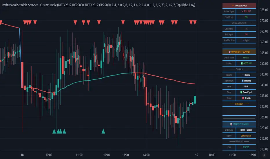
### **Step 2: Understand the Display**
**Chart Elements:**
- **Green/Lime Candles** = Call Option (CE)
- **Pink/Magenta Candles** = Put Option (PE)
- **Brightness** = Activity intensity (brighter = more action!)
- **Triangle Up** = Buy Call Signal ▲
- **Triangle Down** = Buy Put Signal ▼
**Metrics Panel (Bottom Right):**
- **🔥 CE/PE INT**: Intensity score (higher = better)
- **PCR**: Above 1.0 = Bullish, Below 1.0 = Bearish
- **VOL Δ**: Positive = CE volume dominance
- **IV%ile**: Above 70 = High IV (premium sellers advantage)
- **BBW**: Expansion indicator (⚡ = expanding)
- **Momentum**: Price acceleration tracker
### **Step 3: Trading Rules**
**For Buying Calls (Bullish):**
1. Wait for ▲ signal below CE candle
2. Check **CE INT > 40%** (moderate to high activity)
3. Confirm **CE BBW ⚡** (volatility expanding)
4. Verify **CE Mom** positive (momentum building)
5. **Entry**: Current CE premium
6. **Target**: Use Fibonacci levels or book on intensity drop
**For Buying Puts (Bearish):**
1. Wait for ▼ signal above PE candle
2. Check **PE INT > 40%** (moderate to high activity)
3. Confirm **PE BBW ⚡** (volatility expanding)
4. Verify **PE Mom** positive (momentum building)
5. **Entry**: Current PE premium
6. **Target**: Use Fibonacci levels or book on intensity drop
**Risk Management:**
- Avoid trades when intensity < 30% (low liquidity)
- Higher intensity = tighter stops (volatile moves)
- Watch for intensity divergence (price up, intensity down = weakness)
***
## ⚙️ SETTINGS GUIDE
### **Group 1: UNDERLYING & SYMBOL**
- **Underlying**: Main index/stock ticker
- **Option Root**: Symbol prefix (NIFTY, BANKNIFTY, etc.)
- **Strike Interval**: 50 for NIFTY, 100 for BANKNIFTY
- **Expiry Date**: Target expiry (Year/Month/Day)
- **Spot Source**: Auto (First 5m), Live Close, or Manual
### **Group 2: OPTION CHAIN SCANNER**
- **ATM Strike**: Center point for scanning (manually input)
- **Scan Range**: ±N strikes to scan (1-5)
- **Compression Threshold**: Max CE-PE difference % (8% default)
- **Min Volume**: Liquidity filter (100 default)
- **Auto-Select**: Enable for automatic best pair selection
### **Group 3: SIGNAL FILTERS**
- **BBW Length**: Volatility calculation period (20 default)
- **BBW Expansion Threshold**: Multiplier for expansion (1.30x)
- **Min BBW**: Minimum volatility % (2.0%)
- **EMA Filter**: Enable trend confirmation (21 EMA)
- **Delta Momentum**: Require CE > PE momentum for calls (vice versa)
### **Group 4: SIGNAL DISPLAY**
- **Show Buy Signals**: Toggle call/put signals
- Simple triangle markers (▲ for calls, ▼ for puts)
### **Group 5: VISUALIZATION**
- **Plot Candles**: Show CE/PE candlesticks
- **Normalize to % Change**: Compare premiums as % (recommended)
- **Show EMA**: Display trend lines
- **Show Metrics Panel**: Display analytics table
- **Table Position**: Move metrics panel (9 positions)
- **Table Size**: Adjust text size (Tiny to Huge)
### **Group 6: OPTION ANALYTICS**
- **Show PCR**: Put-Call Ratio display
- **Show Volume Analysis**: Volume delta tracking
- **Show IV Percentile**: 1-year IV ranking
### **Group 7: INTENSITY SYSTEM** 🔥
- **Enable Intensity Coloring**: Turn on dynamic brightness
- **Intensity Smoothing**: Higher = smoother (3 default)
- **Volume Weight**: Impact of volume surges (35%)
- **IV/BBW Weight**: Impact of volatility expansion (40%)
- **Movement Weight**: Impact of price acceleration (25%)
- **Min Brightness**: Dimmest state (70% transparency)
- **Max Brightness**: Brightest state (0% = fully opaque)
***
## 🎓 TRADING STRATEGIES
### **Strategy 1: Intensity Breakout**
- Wait for intensity to rise from <30% to >60%
- Enter on signal with bright candle
- Exit when intensity drops below 40%
### **Strategy 2: Volatility Expansion**
- Monitor BBW indicator
- Enter on ⚡ expansion + signal
- Target quick 20-30% premium gains
### **Strategy 3: PCR Contrarian**
- PCR > 1.3 = Oversold (look for call signals)
- PCR < 0.7 = Overbought (look for put signals)
- Combine with intensity confirmation
### **Strategy 4: Volume Delta Momentum**
- Strong positive VOL Δ = CE buying pressure
- Enter calls on dips with high CE intensity
- Vice versa for puts
***
## 📋 SUPPORTED EXCHANGES & SYMBOLS
**Exchanges:**
- NSE (National Stock Exchange of India)
**Supported Underlyings:**
- NIFTY 50
- BANKNIFTY
- FINNIFTY
- MIDCPNIFTY
- Individual stocks with liquid options
**Option Formats:**
- NSE Standard: `NSE:NIFTY251230C25900`
- NSE Weekly: `NSE:NIFTY25DEC25900CE`
- Custom/Broker-Specific formats
***
## ⚡ PERFORMANCE OPTIMIZATION
This indicator is optimized for speed:
- **Tuple-based security requests** (80% faster than standard)
- **Minimal repainting** (signals confirmed on bar close)
- **Efficient array operations**
- **Smart caching** of repeated calculations
- Works smoothly even on 1-minute charts
***
## 🚨 ALERTS
Built-in alert conditions:
- **Buy Call Signal**: Triggered on confirmed call entry
- **Buy Put Signal**: Triggered on confirmed put entry
**Setup:**
1. Click "Create Alert" on TradingView
2. Select "Guru Dronacharya Pro"
3. Choose "Buy Call Signal" or "Buy Put Signal"
4. Set notification method (popup/email/webhook)
***
## ⚠️ RISK DISCLAIMER
**IMPORTANT**: This indicator is for **educational purposes only**.
- Options trading carries substantial risk of loss
- Past performance does not guarantee future results
- Always use proper risk management (stop losses, position sizing)
- No indicator guarantees profitable trades
- Test thoroughly on paper/sim before live trading
- Consult a financial advisor before trading
**The creator is not responsible for any trading losses incurred using this indicator.**
***
## 🔄 VERSION HISTORY
**v1.0 (Current)**
- Initial release
- Dynamic intensity system
- Intelligent strike selection
- Multi-filter signal generation
- Professional analytics panel
- Theme-aware visualization
- Full customization support
***
## 💬 FEEDBACK & SUPPORT
Found this indicator helpful? Please:
- ⭐ Leave a rating
- 💬 Share your experience in comments
- 📊 Publish your chart ideas using this indicator
- 🔔 Follow for updates and new indicators
**Questions?** Drop a comment, and I'll help you optimize your settings!
***
## 🏆 WHO IS THIS FOR?
✅ **Intraday Option Traders** (scalping & day trading)
✅ **Swing Option Traders** (multi-day positions)
✅ **Premium Buyers** (directional option strategies)
✅ **Technical Analysts** (volatility & momentum-based)
✅ **NSE Options Specialists** (NIFTY/BANKNIFTY focused)
❌ **NOT suitable for:**
- Complete beginners (learn basics first)
- Premium sellers (different indicator needed)
- Set-and-forget strategies (requires active monitoring)
***
## 🙏 ACKNOWLEDGMENTS
Named after **Guru Dronacharya**, the legendary teacher from Mahabharata known for precision, discipline, and strategic mastery – qualities every successful trader needs.
**May your trades be profitable and your risk be managed! 🚀**
***
**Tags:** Options Trading, NSE Options, NIFTY Options, BANKNIFTY Options, Option Chain Analysis, Volatility Trading, Intensity System, Indian Stock Market, Intraday Trading, Premium Analysis, PCR Indicator, Options Signals
***
**Legal:** This indicator does not constitute financial advice. All trading decisions are your responsibility. Always trade with risk capital you can afford to lose.
Indicatore Pine Script®