Range Identifier [LazyBear] ---- May 05 2015 -----
Added support for filtered ranges:
RID V3 : pastebin.com
RIDv3 has full backward compatibility (!?), meaning all my descriptions below still apply for V3.
-- In addition, I have added a NON-OVERLAY mode, which can be put in its own pane, that shows the number of bars in the current range.
-- in Overlay mode, you can switch on/off filtering ranges based on the bar count.
Sample chart:
---- April 30 2015 -----
Updated the source to show a connected Midline only when ConnectRanges option is enabled.
Updated src: pastebin.com
Sample chart:
---- Original Desc ----
This is a simple indicator that highlights the price ranges. Very helpful in determining a breakout.
There are many ways to incorporate this in to your strategy. One simple idea could be to buy if the price breaks above a range, when above the specified EMA, and to SELL when it breaks down from a range below the EMA.
All options are configurable. Alerts can be setup using the specified plot names.
By default it shows only the ranges, but can be configured to show the full "channel". Chart below shows connected ranges with highlights ON.
Range highlighting can be turned OFF. Chart below shows that:
Note for the pine coders:
As you probably noticed in the charts above, single range is showing 2 colors(red/green). Fill() doesn't accept a series for colors, so I worked around this using two fill() statements with a moving DUMMY line, to get this mixed color effect.
List of my public indicators: bit.ly
List of my app-store indicators: blog.tradingview.com
Cerca negli script per "2015年黄金价格走势"

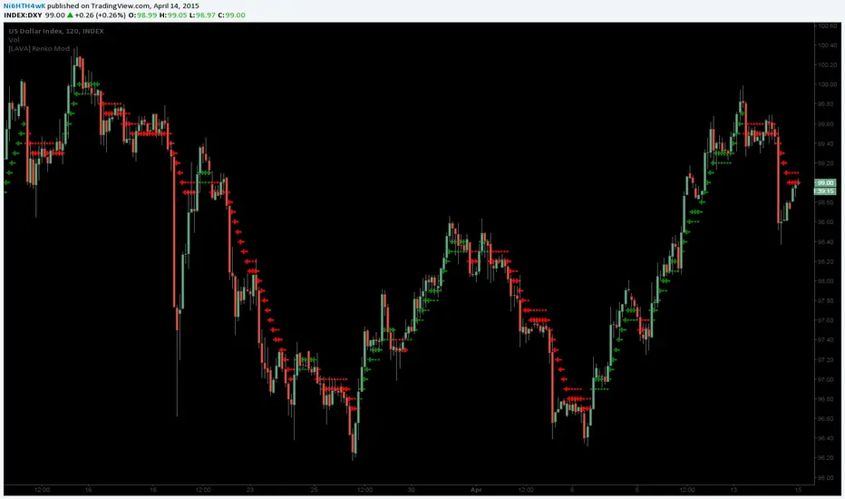
[LAVA] Renko ModTradingview.com Pinescript @author Ni6HTH4wK (LAVA) with assistance from @zmm20
Original code by Richard Santos, (RS)Renko Mod
(RS) www.tradingview.com
(LAVA) 19P7bkzqSAwSm6X7tXmRVkx6AuBXEUZioo
Traditional cross and circles view displayed here, but my favorite look is small linebreak and circles.
Different views available...
Type 2 -
Type 1 -
Without barcoloring -
**EDIT**
pastebin.com - Fixes missed bottoms / tops (April 15th, 2015)
pastebin.com - Fixes slow recognition of steep movements (April 25th, 2015)
Value Chart [TMC]*** April 20, 2015 - NEW UPDATE ***
Added classic color scheme and additional lines. Updated source: pastebin.com
April 10, 2015 - Updated version of Value Chart - candles draw correctly now.
Requires cover layer to be set as same color as your background. (white in default)
I hope you will enjoy it. :)

McCrayTrendTraders often rely on price breaking above or below the 50-day moving average (50D-MA) as a buy/sell signal. However, this approach frequently results in false breakouts, especially during low-volatility periods when price compression precedes major moves. To address this issue, we use an 8-day exponential moving average (8D-EMA) to represent price and focus on the crossovers between the 8D-EMA and the 48D-EMA as entry/exit signals. This method reduces noise in low-volatility conditions, enables earlier trend entries, and helps traders stay in trends longer.
The indicator incorporates a 111-day EMA (111D-EMA) to define market bias:
• Above the 111D-EMA: Bias is long, favoring buying and selling into cash.
• Below the 111D-EMA: Bias is short, favoring selling and buying into cash.
An exception to this rule occurs when a bullish cross happens within 40% of the 200-week moving average (200W-MA), as these conditions historically signal optimal times to acquire BTC.
Signals:
Buy signals:
• A bullish cross while price is above the 111D-EMA.
• A bullish cross near the 200W-MA threshold (optional setting).
Sell signals:
• A bearish cross while price is below the 111D-EMA.
Exit signals:
• Both EMAs turn red (for long trades) or green (for short trades).
• The shading between the 111D-EMA and 200W-MA turns red (for longs) or green (for shorts), if enabled.
Reversal opportunities:
• A buy or sell label during an exit signal may indicate a reversal point, allowing traders to take profit and reopen positions in the opposite direction.
The methodology behind this indicator has generated 132% alpha since October 6, 2015. Special thanks to Anurag Parashar for refining the stylistic elements of the indicator.

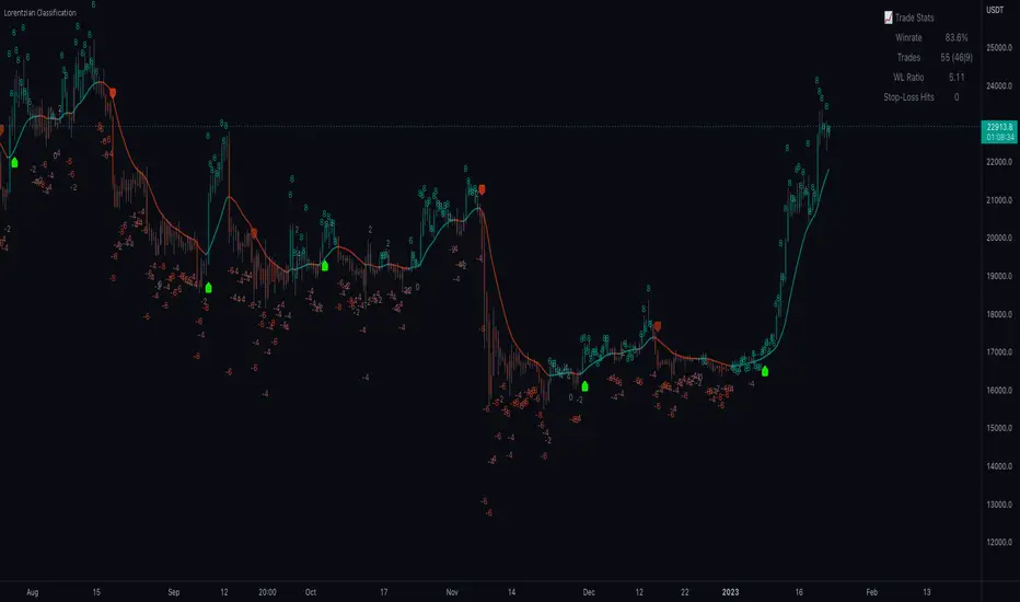
Machine Learning: Lorentzian Classification█ OVERVIEW
A Lorentzian Distance Classifier (LDC) is a Machine Learning classification algorithm capable of categorizing historical data from a multi-dimensional feature space. This indicator demonstrates how Lorentzian Classification can also be used to predict the direction of future price movements when used as the distance metric for a novel implementation of an Approximate Nearest Neighbors (ANN) algorithm.
█ BACKGROUND
In physics, Lorentzian space is perhaps best known for its role in describing the curvature of space-time in Einstein's theory of General Relativity (2). Interestingly, however, this abstract concept from theoretical physics also has tangible real-world applications in trading.
Recently, it was hypothesized that Lorentzian space was also well-suited for analyzing time-series data (4), (5). This hypothesis has been supported by several empirical studies that demonstrate that Lorentzian distance is more robust to outliers and noise than the more commonly used Euclidean distance (1), (3), (6). Furthermore, Lorentzian distance was also shown to outperform dozens of other highly regarded distance metrics, including Manhattan distance, Bhattacharyya similarity, and Cosine similarity (1), (3). Outside of Dynamic Time Warping based approaches, which are unfortunately too computationally intensive for PineScript at this time, the Lorentzian Distance metric consistently scores the highest mean accuracy over a wide variety of time series data sets (1).
Euclidean distance is commonly used as the default distance metric for NN-based search algorithms, but it may not always be the best choice when dealing with financial market data. This is because financial market data can be significantly impacted by proximity to major world events such as FOMC Meetings and Black Swan events. This event-based distortion of market data can be framed as similar to the gravitational warping caused by a massive object on the space-time continuum. For financial markets, the analogous continuum that experiences warping can be referred to as "price-time".
Below is a side-by-side comparison of how neighborhoods of similar historical points appear in three-dimensional Euclidean Space and Lorentzian Space:
This figure demonstrates how Lorentzian space can better accommodate the warping of price-time since the Lorentzian distance function compresses the Euclidean neighborhood in such a way that the new neighborhood distribution in Lorentzian space tends to cluster around each of the major feature axes in addition to the origin itself. This means that, even though some nearest neighbors will be the same regardless of the distance metric used, Lorentzian space will also allow for the consideration of historical points that would otherwise never be considered with a Euclidean distance metric.
Intuitively, the advantage inherent in the Lorentzian distance metric makes sense. For example, it is logical that the price action that occurs in the hours after Chairman Powell finishes delivering a speech would resemble at least some of the previous times when he finished delivering a speech. This may be true regardless of other factors, such as whether or not the market was overbought or oversold at the time or if the macro conditions were more bullish or bearish overall. These historical reference points are extremely valuable for predictive models, yet the Euclidean distance metric would miss these neighbors entirely, often in favor of irrelevant data points from the day before the event. By using Lorentzian distance as a metric, the ML model is instead able to consider the warping of price-time caused by the event and, ultimately, transcend the temporal bias imposed on it by the time series.
For more information on the implementation details of the Approximate Nearest Neighbors (ANN) algorithm used in this indicator, please refer to the detailed comments in the source code.
█ HOW TO USE
Below is an explanatory breakdown of the different parts of this indicator as it appears in the interface:
Below is an explanation of the different settings for this indicator:
General Settings:
Source - This has a default value of "hlc3" and is used to control the input data source.
Neighbors Count - This has a default value of 8, a minimum value of 1, a maximum value of 100, and a step of 1. It is used to control the number of neighbors to consider.
Max Bars Back - This has a default value of 2000.
Feature Count - This has a default value of 5, a minimum value of 2, and a maximum value of 5. It controls the number of features to use for ML predictions.
Color Compression - This has a default value of 1, a minimum value of 1, and a maximum value of 10. It is used to control the compression factor for adjusting the intensity of the color scale.
Show Exits - This has a default value of false. It controls whether to show the exit threshold on the chart.
Use Dynamic Exits - This has a default value of false. It is used to control whether to attempt to let profits ride by dynamically adjusting the exit threshold based on kernel regression.
Feature Engineering Settings:
Note: The Feature Engineering section is for fine-tuning the features used for ML predictions. The default values are optimized for the 4H to 12H timeframes for most charts, but they should also work reasonably well for other timeframes. By default, the model can support features that accept two parameters (Parameter A and Parameter B, respectively). Even though there are only 4 features provided by default, the same feature with different settings counts as two separate features. If the feature only accepts one parameter, then the second parameter will default to EMA-based smoothing with a default value of 1. These features represent the most effective combination I have encountered in my testing, but additional features may be added as additional options in the future.
Feature 1 - This has a default value of "RSI" and options are: "RSI", "WT", "CCI", "ADX".
Feature 2 - This has a default value of "WT" and options are: "RSI", "WT", "CCI", "ADX".
Feature 3 - This has a default value of "CCI" and options are: "RSI", "WT", "CCI", "ADX".
Feature 4 - This has a default value of "ADX" and options are: "RSI", "WT", "CCI", "ADX".
Feature 5 - This has a default value of "RSI" and options are: "RSI", "WT", "CCI", "ADX".
Filters Settings:
Use Volatility Filter - This has a default value of true. It is used to control whether to use the volatility filter.
Use Regime Filter - This has a default value of true. It is used to control whether to use the trend detection filter.
Use ADX Filter - This has a default value of false. It is used to control whether to use the ADX filter.
Regime Threshold - This has a default value of -0.1, a minimum value of -10, a maximum value of 10, and a step of 0.1. It is used to control the Regime Detection filter for detecting Trending/Ranging markets.
ADX Threshold - This has a default value of 20, a minimum value of 0, a maximum value of 100, and a step of 1. It is used to control the threshold for detecting Trending/Ranging markets.
Kernel Regression Settings:
Trade with Kernel - This has a default value of true. It is used to control whether to trade with the kernel.
Show Kernel Estimate - This has a default value of true. It is used to control whether to show the kernel estimate.
Lookback Window - This has a default value of 8 and a minimum value of 3. It is used to control the number of bars used for the estimation. Recommended range: 3-50
Relative Weighting - This has a default value of 8 and a step size of 0.25. It is used to control the relative weighting of time frames. Recommended range: 0.25-25
Start Regression at Bar - This has a default value of 25. It is used to control the bar index on which to start regression. Recommended range: 0-25
Display Settings:
Show Bar Colors - This has a default value of true. It is used to control whether to show the bar colors.
Show Bar Prediction Values - This has a default value of true. It controls whether to show the ML model's evaluation of each bar as an integer.
Use ATR Offset - This has a default value of false. It controls whether to use the ATR offset instead of the bar prediction offset.
Bar Prediction Offset - This has a default value of 0 and a minimum value of 0. It is used to control the offset of the bar predictions as a percentage from the bar high or close.
Backtesting Settings:
Show Backtest Results - This has a default value of true. It is used to control whether to display the win rate of the given configuration.
█ WORKS CITED
(1) R. Giusti and G. E. A. P. A. Batista, "An Empirical Comparison of Dissimilarity Measures for Time Series Classification," 2013 Brazilian Conference on Intelligent Systems, Oct. 2013, DOI: 10.1109/bracis.2013.22.
(2) Y. Kerimbekov, H. Ş. Bilge, and H. H. Uğurlu, "The use of Lorentzian distance metric in classification problems," Pattern Recognition Letters, vol. 84, 170–176, Dec. 2016, DOI: 10.1016/j.patrec.2016.09.006.
(3) A. Bagnall, A. Bostrom, J. Large, and J. Lines, "The Great Time Series Classification Bake Off: An Experimental Evaluation of Recently Proposed Algorithms." ResearchGate, Feb. 04, 2016.
(4) H. Ş. Bilge, Yerzhan Kerimbekov, and Hasan Hüseyin Uğurlu, "A new classification method by using Lorentzian distance metric," ResearchGate, Sep. 02, 2015.
(5) Y. Kerimbekov and H. Şakir Bilge, "Lorentzian Distance Classifier for Multiple Features," Proceedings of the 6th International Conference on Pattern Recognition Applications and Methods, 2017, DOI: 10.5220/0006197004930501.
(6) V. Surya Prasath et al., "Effects of Distance Measure Choice on KNN Classifier Performance - A Review." .
█ ACKNOWLEDGEMENTS
@veryfid - For many invaluable insights, discussions, and advice that helped to shape this project.
@capissimo - For open sourcing his interesting ideas regarding various KNN implementations in PineScript, several of which helped inspire my original undertaking of this project.
@RikkiTavi - For many invaluable physics-related conversations and for his helping me develop a mechanism for visualizing various distance algorithms in 3D using JavaScript
@jlaurel - For invaluable literature recommendations that helped me to understand the underlying subject matter of this project.
@annutara - For help in beta-testing this indicator and for sharing many helpful ideas and insights early on in its development.
@jasontaylor7 - For helping to beta-test this indicator and for many helpful conversations that helped to shape my backtesting workflow
@meddymarkusvanhala - For helping to beta-test this indicator
@dlbnext - For incredibly detailed backtesting testing of this indicator and for sharing numerous ideas on how the user experience could be improved.
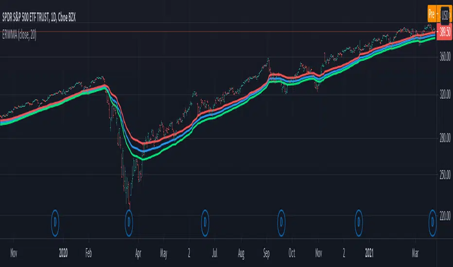
Elastic Range Weighted Moving AverageThis indicator is similar to the Elastic Volume Weighted Moving Average, except it uses True Range instead of Volume.
This can be useful where volume data is unavailable (for instance, in forex), or if prices moved way too fast, such as the Swiss franc crash back in 2015.
Comparison:
Let me know if you want more features added to this indicator. I'll see what I can do.
Your feedback is always appreciated. Thank you.
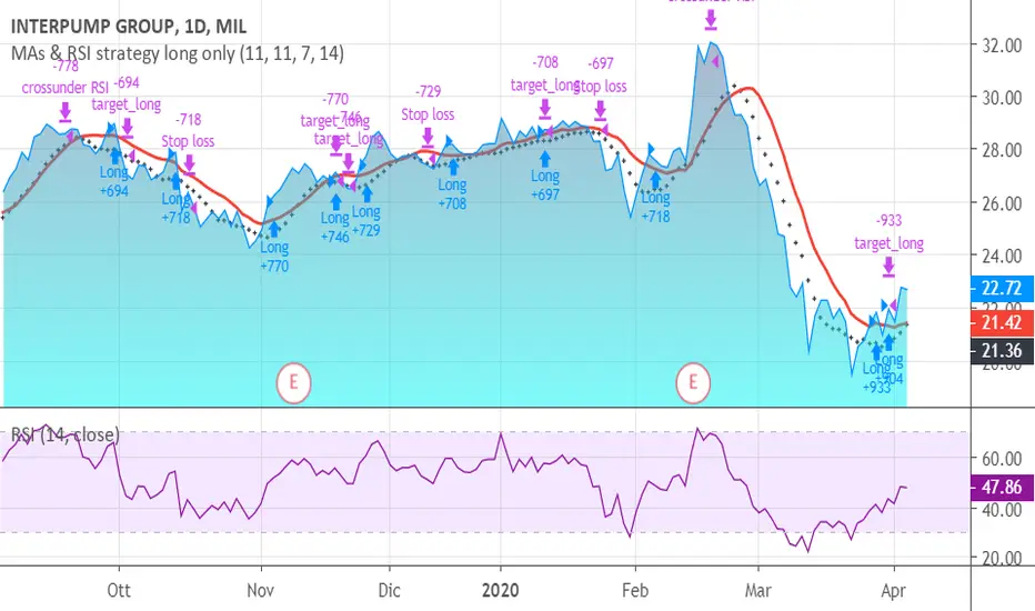
MAs & RSI strategy long onlyThis system originates from many articles by Enrico Malverti, Trading System, 2015.
Many trading systems are more stable if you use simple and not so innovative indicators, like exponential moving averages and Relative Strengthe index.
Differently by the original article:
- there is no ATR Filter, but we have introduced a Schaff Indicator. If you have multiple shares/commodities to choose, prefer what has a better value of Schaff;
- there is no fixed stop loss but a second moving average (fast), used as target. There are also Simple Mov Averages on lows (trailing stop loss for long) and a SMA on highs (trailing stop loss for short position).
Be careful, in the system only long case, because being short is not the reverse of being long (as stated in my blog)
SMA on highs are therefore only graphically put.
In this version, I’ve changed the “religious” use of EMAs (“sponsored by” Alexander Elder) to “ordinary” MAs: this because since simple moving averages measure all the factor in addition egual each one, this involve a sort of “offset” in the graph, while EMAs give a major “importance” to the last value (last close itself, you’re already considering): therefore this calculation may be counterproductive.
HOW TO OPERATE
BUY when prices crosses over SMAon long period (we suggest, however, sma long = Sma fast period = no. 11 for italian and european shares)
SELL when
prices go under SMA on lows (7 period), or under on SMA fast!
RSI crosses under level 70 or is higher than 75 (or 80, but in code there is 75)
Optimal 4H Moving Average Ribbon
Stolen from Madrid Moving Average Ribbon : 2.0 : MMAR - Respect!
madridjourneyonws.blogspot.com
Adapted for 4H 5 most optimal EMAs
This plots a moving average ribbon, please use the exponential not the standard.
It is based on a constant calculation of the most profitable EMAs to trade on the 4H time frame for Bitcoin!
Thus the values will be updated with time as they change.
As an example trading the EMA 44 will return ~12000% on initial investment from begining of 2015. Hodl would have given "just" ~4150% for same period!
It is a simple price breaks above EMAs to go long and break below to go short strategy.
This study is best viewed with a dark background. It provides an easy
and fast way to determine the trend direction and possible reversals.

Outsidebar vs Insidebar, Illusion Strategy (by ChartArt)WARNING: This strategy does not work! Please don't trade with this strategy
I'm sharing this strategy for the following three educational reasons:
1. You can easily find 100% strategies, but if they only seem to work 100% on one asset, they actually don't work at all. Therefore never backtest your strategy only on one asset, especially forward testing is useless, because it tends to repeat the old patterns. Your strategy has to work on as many different assets as possible.
2. The pyramiding of orders can have an impact on the strategy. In this case if you manually change the strategy settings by increasing it from 1 to 100 pyramiding orders changes the percent profitable on "UKOIL" monthly from 100% to 90% profitable. On other assets you can see very different results. Allowing much more pyramiding orders in this case results in opening orders where the background color highlights appear.
3. The Tradingview backtest beta version currently does not close the last open trade during the backtest. In this case going long on "UKOIL" near the top in 2011 as this strategy did would result in a big loss in 2015. But since the trade is still open and not canceled out by a new short order it still appears as if this strategy works 100% profitable. Which it doesn't.

Bias + VWAP Pullback — v4 (PA + BOS/CHOCH)Simple idea: I identify the trend (bias) from the larger timeframe, and only trade pullbacks to the VWAP/EMA during liquidity (London/New York). When the trend is clear, gold moves strongly, and its pullbacks to the balance lines provide clear opportunities.
Timeframe and Sessions (Cairo Time)
Analysis: H1 to determine the trend.
Implementation: 5m (or 1m if professional).
Trading window:
London Opening: 10:00–12:30
New York Opening: 16:30–19:00
(avoid the rest of the day unless there is exceptional traffic).
Direction determination (BIAS)
On H1:
If the price is above the 200 EMA and the daily VWAP is bullish and the price is above it → uptrend (long-only).
If the price is below the 200 EMA and the daily VWAP is bearish and the price is below it → bearish trend (short-only).
Determine your levels: yesterday's high/low (PDH/PDL) + approximate Asia range (03:00–09:30).
Entry Rules (Setup A: Trend Continuation)
Asia range breakout towards Bias during liquidity window.
Wait for a withdrawal to:
Daily VWAP, or
EMA50 on 5m frame (best if both cross).
Confirmation: Confirmation low/high on 5m (HL buy/LH sell) + clear impulse candle (Body is greater than average of last 10 candles).
Entry:
Buy: When the price returns above VWAP/EMA50 with a confirmation candle close.
Sell: The exact opposite.
Stop Loss (SL): Below/above the last confirmation low/high or ATR(14, 5m) x 1.5 (largest).
Objectives:
TP1 = 1R (Close 50% and move the rest Break-even).
TP2 = 2.5R to 3R or at an important HTF level (PDH/PDL/Bid/Demand Zone).
Entry Rules (Setup B: Reversion to VWAP – “Mean Reversion”)
Use with extreme caution, once daily maximum:
Price deviation from VWAP by more than ~1.5 x ATR(14, 5m) with rejection candles appearing near PDH/PDL.
Reverse entry towards the return of VWAP.
SL small behind rejection top/bottom.
Main target: VWAP. (Don't get greedy — this scenario is for extended periods only.)
News Filtering and Risk Management
Avoid trading 15–30 minutes before/after strong US news (CPI, NFP, FOMC).
Maximum daily loss: 1.5–2% of account balance.
Risk per trade: 0.25–0.5% (if you are learning) or 0.5–1% (if you are experienced).
Do not exceed two consecutive losing trades per day.
Don't chase the market after the opportunity has passed — wait for the next pullback.
Smart Deal Management
After TP1: Move stop to entry point + trail the rest with EMA20 on 5m or ATR Trailing = ATR(14)×1.0.
If the price touches a strong daily level (PDH/PDL) and fails to break, consider taking additional profit.
If VWAP starts to flatten and breaks against the trend on H1, stop trading for the day.
Quick Checklist (Before Entry)
H1 trend is clear and consistent with 200EMA + VWAP.
Penetrating the Asia range towards Bias.
Clean pull to VWAP/EMA50 on 5m.
Confirmation candle and real push.
SL is logical (behind swing/ATR×1.5) and R :R ≥ 1:2.
No red news coming soon.
Example of "ready-made" settings
EMA: 20, 50, 200 on 5m, 200 only on H1.
VWAP: Daily (reset daily).
ATR: 14 on 5m.
Levels: PDH/PDL + Asia Band (03:00–09:30 Cairo).
Gold Notes
Gold is fast and sharp at the open; don't get in early — wait for the draw.
Fakeouts are common before news: it is best to call with the trend after the price returns above/below VWAP.
Don't expect 80% consistent wins every day — the advantage comes from discipline, filtering out bad days, and only withdrawing when you're on the right track.
تعتبر شركة الماسة الألمانية أحد المؤسسات العاملة بالمملكة العربية السعودية ولها تاريخ طويل من الخدمات الكثيرة والمتنوعة التى مازالت تقدمها للكثير من العملاء داخل جميع مدن وأحياء المملكة حيث نقدم أفضل ما لدينا من خلال مجموعة الشركات التالية والتي من خلالها ستتلقي كل ما تحتاج إلية في كل المجال المختلفة فنحن نعمل منذ عام 2015 ولنا سابقات اعمال فى مختلف المجالات الحيوية التى نخدم من خلالها عملائنا ونوفر لهم أرخص الأسعار وبأعلى جودة من الممكن توفرها فى المجالات التالية :-
خدمات تنظيف المنازل والفلل والشقق
خدمات عزل الخزانات تنظيف غسيل صيانة اصلاح
خدمات جلي البلاط والرخام والسيراميك
خدمات نقل العفش عمالة فلبينية مدربة
خدمات مكافحة الحشرات بجدة
كل هذة الخدمات وأكثر نوفرها لكل المتعاقدين بأفضل الطرق مع توفير خطط وبرامج متنوعة لأتمام العمل المسنود إلينا بأفضل وأحدث الطرق الحديثة والعصرية سواء فى شركات النظافة بجدة ومكة المكرمة أو شركات نقل العفش بجدة عمالة فلبينية وباقى الخدمات مثل جلي وتلميع الرخام بمكة وجدة ولا ننسي شركة مكافحة حشرات بجدة التى ساعدت آلاف المواطنين على تنظيف منازلهم من الحشرات بأفضل مبيدات حشرية.

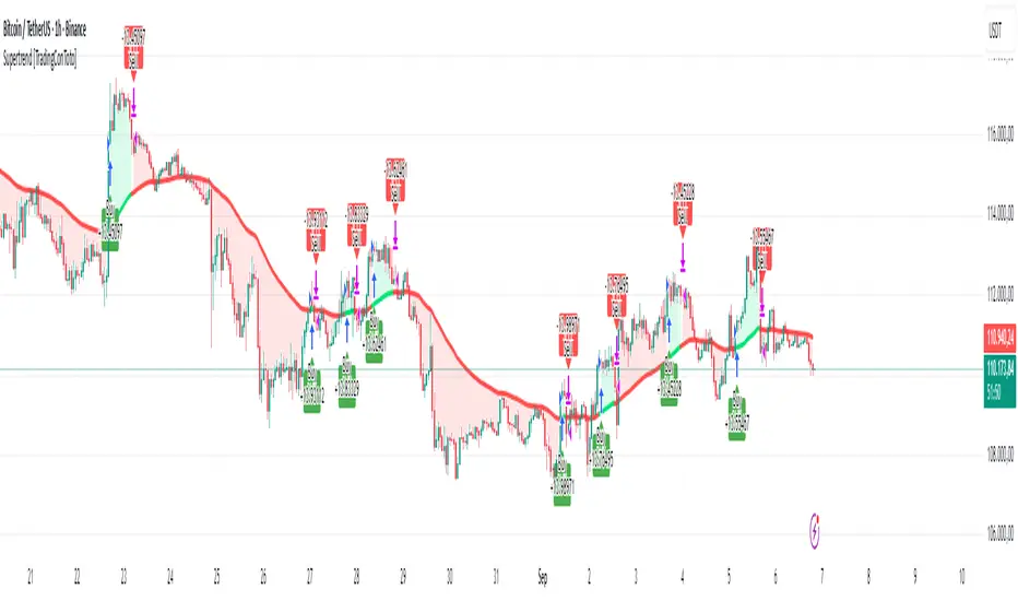
Supertrend [TradingConToto]Supertrend — ADX/DI + EMA Gap + Breakout (with Mobile UI)
What makes it original
Supertrend combines trend strength (ADX/DI), multi-timeframe bias (EMA63 and EMA 200D equivalent), a structural filter based on the distance between EMA2400 and EMA4800 expressed in ATR units, and a momentum confirmation through a previous high breakout.
This is not a random mashup — it’s a sequence of filters designed to reduce trades in ranging markets and prioritize mature trends:
Direction: +DI > -DI (trend led by buyers).
Strength: ADX > mean(ADX) (avoids weak, choppy phases).
Short-term bias: Close > EMA63.
Long-term bias: Close > EMA4800 ≈ EMA200 daily on H1.
Momentum: Close > High (immediate breakout).
Structure: (EMA2400 − EMA4800) > k·ATR (ensures separation in ATR units, filters out flat phases).
Entries & exits
Entry: when all six conditions are met and no open position exists.
Exit: if +DI < -DI or Close < EMA63.
Visuals: EMA63 is painted green while in position and red otherwise, with a supertrend-style band; “BUY” labels appear below the green band and “SELL” labels above the red band.
UI: includes a compact table (mobile-friendly) showing the state of each condition.
Default parameters used in this publication
Initial capital: 10,000
Position size: 10% of equity (≤10% per trade is considered sustainable).
Commission: 0.01% per side (adjust to your broker/market).
Slippage: 1 tick
Pyramiding: 0 (only one position at a time)
Adjust commission/slippage to match your market. For US equities, commissions are often per share; for spot crypto, 0.10–0.20% total is common. I publish with 0.01% per side as a conservative example to avoid overestimating results.
Recommended backtest dataset
Timeframe: H1
Multi-cycle window (e.g. 2015–today)
Symbols with high liquidity (e.g. NASDAQ-100 large caps, or BTC/ETH spot) to generate 100+ trades. Avoid cherry-picked short windows.
Why each filter matters
+DI > -DI + ADX > mean: reduce counter-trend trades and weak signals.
Close > EMA63 + Close > EMA4800: enforce trend alignment in short and long horizons.
Breakout High : requires immediate momentum, avoids early entries.
EMA gap in ATR units: blocks flat or compressed structures where EMA200D aligns with price.
Limitations
The breakout filter may skip healthy pullbacks; the design prioritizes continuation over perfect entry price.
No fixed trailing stop/TP; exits depend on trend degradation via DI/EMA63.
Results vary with real costs (commissions, slippage, funding). Adjust defaults to your broker.
How to use
Apply it on a clean chart (no other indicators when publishing).
Keep in mind the default parameters above; if you change them, mention it in your notes and use the same values in the Strategy Tester.
Ensure your dataset produces 100+ trades for statistical validity.
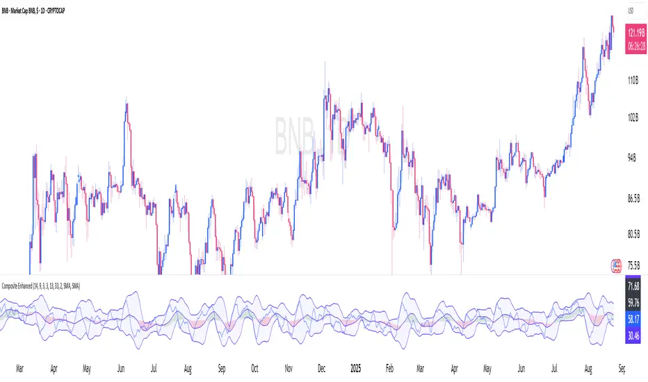
Constance Brown Composite Index EnhancedWhat This Indicator Does
Implements Constance Brown's copyrighted Composite Index formula (1996) from her Master's thesis - a breakthrough oscillator that solves the critical problem where RSI fails to show divergences in long-horizon trends, providing early warning signals for major market reversals.
The Problem It Solves
Traditional RSI frequently fails to display divergence signals in Global Equity Indexes and long-term charts, leaving asset managers without warning of major price reversals. Brown's research showed RSI failed to provide divergence signals 42 times across major markets - failures that would have been "extremely costly for asset managers."
Key Components
Composite Line: RSI Momentum (9-period) + Smoothed RSI Average - the core breakthrough formula
Fast/Slow Moving Averages: Trend direction confirmation (13/33 periods default)
Bollinger Bands: Volatility envelope around the composite signal
Enhanced Divergence Detection: Significantly improved trend reversal timing vs standard RSI
Research-Proven Performance
Based on Brown's extensive study across 6 major markets (1919-2015):
42 divergence signals triggered where RSI showed none
33 signals passed with meaningful reversals (78% success rate)
Only 5 failures - exceptional performance in monthly/2-month timeframes
Tested on: German DAX, French CAC 40, Shanghai Composite, Dow Jones, US/Japanese Government Bonds
New Customization Features
Moving Average Types: Choose SMA or EMA for fast/slow lines
Optional Fills: Toggle composite and Bollinger band fills on/off
All Periods Adjustable: RSI length, momentum, smoothing periods
Visual Styling: Customize colors and line widths in Style tab
Default Settings (Original Formula)
RSI Length: 14
RSI Momentum: 9 periods
RSI MA Length: 3
SMA Length: 3
Fast SMA: 13, Slow SMA: 33
Bollinger STD: 2.0
Applications
Long-term investing: Monthly/2-month charts for major trend changes
Elliott Wave analysis: Maximum displacement at 3rd-of-3rd waves, divergence at 5th waves
Multi-timeframe: Pairs well with MACD, works across all timeframes
Global markets: Proven effective on equities, bonds, currencies, commodities
Perfect for serious traders and asset managers seeking the proven mathematical edge that traditional RSI cannot provide.
Ray Dalio's All Weather Strategy - Portfolio CalculatorTHE ALL WEATHER STRATEGY INDICATOR: A GUIDE TO RAY DALIO'S LEGENDARY PORTFOLIO APPROACH
Introduction: The Genesis of Financial Resilience
In the sprawling corridors of Bridgewater Associates, the world's largest hedge fund managing over 150 billion dollars in assets, Ray Dalio conceived what would become one of the most influential investment strategies of the modern era. The All Weather Strategy, born from decades of market observation and rigorous backtesting, represents a paradigm shift from traditional portfolio construction methods that have dominated Wall Street since Harry Markowitz's seminal work on Modern Portfolio Theory in 1952.
Unlike conventional approaches that chase returns through market timing or stock picking, the All Weather Strategy embraces a fundamental truth that has humbled countless investors throughout history: nobody can consistently predict the future direction of markets. Instead of fighting this uncertainty, Dalio's approach harnesses it, creating a portfolio designed to perform reasonably well across all economic environments, hence the evocative name "All Weather."
The strategy emerged from Bridgewater's extensive research into economic cycles and asset class behavior, culminating in what Dalio describes as "the Holy Grail of investing" in his bestselling book "Principles" (Dalio, 2017). This Holy Grail isn't about achieving spectacular returns, but rather about achieving consistent, risk-adjusted returns that compound steadily over time, much like the tortoise defeating the hare in Aesop's timeless fable.
HISTORICAL DEVELOPMENT AND EVOLUTION
The All Weather Strategy's origins trace back to the tumultuous economic periods of the 1970s and 1980s, when traditional portfolio construction methods proved inadequate for navigating simultaneous inflation and recession. Raymond Thomas Dalio, born in 1949 in Queens, New York, founded Bridgewater Associates from his Manhattan apartment in 1975, initially focusing on currency and fixed-income consulting for corporate clients.
Dalio's early experiences during the 1970s stagflation period profoundly shaped his investment philosophy. Unlike many of his contemporaries who viewed inflation and deflation as opposing forces, Dalio recognized that both conditions could coexist with either economic growth or contraction, creating four distinct economic environments rather than the traditional two-factor models that dominated academic finance.
The conceptual breakthrough came in the late 1980s when Dalio began systematically analyzing asset class performance across different economic regimes. Working with a small team of researchers, Bridgewater developed sophisticated models that decomposed economic conditions into growth and inflation components, then mapped historical asset class returns against these regimes. This research revealed that traditional portfolio construction, heavily weighted toward stocks and bonds, left investors vulnerable to specific economic scenarios.
The formal All Weather Strategy emerged in 1996 when Bridgewater was approached by a wealthy family seeking a portfolio that could protect their wealth across various economic conditions without requiring active management or market timing. Unlike Bridgewater's flagship Pure Alpha fund, which relied on active trading and leverage, the All Weather approach needed to be completely passive and unleveraged while still providing adequate diversification.
Dalio and his team spent months developing and testing various allocation schemes, ultimately settling on the 30/40/15/7.5/7.5 framework that balances risk contributions rather than dollar amounts. This approach was revolutionary because it focused on risk budgeting—ensuring that no single asset class dominated the portfolio's risk profile—rather than the traditional approach of equal dollar allocations or market-cap weighting.
The strategy's first institutional implementation began in 1996 with a family office client, followed by gradual expansion to other wealthy families and eventually institutional investors. By 2005, Bridgewater was managing over $15 billion in All Weather assets, making it one of the largest systematic strategy implementations in institutional investing.
The 2008 financial crisis provided the ultimate test of the All Weather methodology. While the S&P 500 declined by 37% and many hedge funds suffered double-digit losses, the All Weather strategy generated positive returns, validating Dalio's risk-balancing approach. This performance during extreme market stress attracted significant institutional attention, leading to rapid asset growth in subsequent years.
The strategy's theoretical foundations evolved throughout the 2000s as Bridgewater's research team, led by co-chief investment officers Greg Jensen and Bob Prince, refined the economic framework and incorporated insights from behavioral economics and complexity theory. Their research, published in numerous institutional white papers, demonstrated that traditional portfolio optimization methods consistently underperformed simpler risk-balanced approaches across various time periods and market conditions.
Academic validation came through partnerships with leading business schools and collaboration with prominent economists. The strategy's risk parity principles influenced an entire generation of institutional investors, leading to the creation of numerous risk parity funds managing hundreds of billions in aggregate assets.
In recent years, the democratization of sophisticated financial tools has made All Weather-style investing accessible to individual investors through ETFs and systematic platforms. The availability of high-quality, low-cost ETFs covering each required asset class has eliminated many of the barriers that previously limited sophisticated portfolio construction to institutional investors.
The development of advanced portfolio management software and platforms like TradingView has further democratized access to institutional-quality analytics and implementation tools. The All Weather Strategy Indicator represents the culmination of this trend, providing individual investors with capabilities that previously required teams of portfolio managers and risk analysts.
Understanding the Four Economic Seasons
The All Weather Strategy's theoretical foundation rests on Dalio's observation that all economic environments can be characterized by two primary variables: economic growth and inflation. These variables create four distinct "economic seasons," each favoring different asset classes. Rising growth benefits stocks and commodities, while falling growth favors bonds. Rising inflation helps commodities and inflation-protected securities, while falling inflation benefits nominal bonds and stocks.
This framework, detailed extensively in Bridgewater's research papers from the 1990s, suggests that by holding assets that perform well in each economic season, an investor can create a portfolio that remains resilient regardless of which season unfolds. The elegance lies not in predicting which season will occur, but in being prepared for all of them simultaneously.
Academic research supports this multi-environment approach. Ang and Bekaert (2002) demonstrated that regime changes in economic conditions significantly impact asset returns, while Fama and French (2004) showed that different asset classes exhibit varying sensitivities to economic factors. The All Weather Strategy essentially operationalizes these academic insights into a practical investment framework.
The Original All Weather Allocation: Simplicity Masquerading as Sophistication
The core All Weather portfolio, as implemented by Bridgewater for institutional clients and later adapted for retail investors, maintains a deceptively simple static allocation: 30% stocks, 40% long-term bonds, 15% intermediate-term bonds, 7.5% commodities, and 7.5% Treasury Inflation-Protected Securities (TIPS). This allocation may appear arbitrary to the uninitiated, but each percentage reflects careful consideration of historical volatilities, correlations, and economic sensitivities.
The 30% stock allocation provides growth exposure while limiting the portfolio's overall volatility. Stocks historically deliver superior long-term returns but with significant volatility, as evidenced by the Standard & Poor's 500 Index's average annual return of approximately 10% since 1926, accompanied by standard deviation exceeding 15% (Ibbotson Associates, 2023). By limiting stock exposure to 30%, the portfolio captures much of the equity risk premium while avoiding excessive volatility.
The combined 55% allocation to bonds (40% long-term plus 15% intermediate-term) serves as the portfolio's stabilizing force. Long-term bonds provide substantial interest rate sensitivity, performing well during economic slowdowns when central banks reduce rates. Intermediate-term bonds offer a balance between interest rate sensitivity and reduced duration risk. This bond-heavy allocation reflects Dalio's insight that bonds typically exhibit lower volatility than stocks while providing essential diversification benefits.
The 7.5% commodities allocation addresses inflation protection, as commodity prices typically rise during inflationary periods. Historical analysis by Bodie and Rosansky (1980) demonstrated that commodities provide meaningful diversification benefits and inflation hedging capabilities, though with considerable volatility. The relatively small allocation reflects commodities' high volatility and mixed long-term returns.
Finally, the 7.5% TIPS allocation provides explicit inflation protection through government-backed securities whose principal and interest payments adjust with inflation. Introduced by the U.S. Treasury in 1997, TIPS have proven effective inflation hedges, though they underperform nominal bonds during deflationary periods (Campbell & Viceira, 2001).
Historical Performance: The Evidence Speaks
Analyzing the All Weather Strategy's historical performance reveals both its strengths and limitations. Using monthly return data from 1970 to 2023, spanning over five decades of varying economic conditions, the strategy has delivered compelling risk-adjusted returns while experiencing lower volatility than traditional stock-heavy portfolios.
During this period, the All Weather allocation generated an average annual return of approximately 8.2%, compared to 10.5% for the S&P 500 Index. However, the strategy's annual volatility measured just 9.1%, substantially lower than the S&P 500's 15.8% volatility. This translated to a Sharpe ratio of 0.67 for the All Weather Strategy versus 0.54 for the S&P 500, indicating superior risk-adjusted performance.
More impressively, the strategy's maximum drawdown over this period was 12.3%, occurring during the 2008 financial crisis, compared to the S&P 500's maximum drawdown of 50.9% during the same period. This drawdown mitigation proves crucial for long-term wealth building, as Stein and DeMuth (2003) demonstrated that avoiding large losses significantly impacts compound returns over time.
The strategy performed particularly well during periods of economic stress. During the 1970s stagflation, when stocks and bonds both struggled, the All Weather portfolio's commodity and TIPS allocations provided essential protection. Similarly, during the 2000-2002 dot-com crash and the 2008 financial crisis, the portfolio's bond-heavy allocation cushioned losses while maintaining positive returns in several years when stocks declined significantly.
However, the strategy underperformed during sustained bull markets, particularly the 1990s technology boom and the 2010s post-financial crisis recovery. This underperformance reflects the strategy's conservative nature and diversified approach, which sacrifices potential upside for downside protection. As Dalio frequently emphasizes, the All Weather Strategy prioritizes "not losing money" over "making a lot of money."
Implementing the All Weather Strategy: A Practical Guide
The All Weather Strategy Indicator transforms Dalio's institutional-grade approach into an accessible tool for individual investors. The indicator provides real-time portfolio tracking, rebalancing signals, and performance analytics, eliminating much of the complexity traditionally associated with implementing sophisticated allocation strategies.
To begin implementation, investors must first determine their investable capital. As detailed analysis reveals, the All Weather Strategy requires meaningful capital to implement effectively due to transaction costs, minimum investment requirements, and the need for precise allocations across five different asset classes.
For portfolios below $50,000, the strategy becomes challenging to implement efficiently. Transaction costs consume a disproportionate share of returns, while the inability to purchase fractional shares creates allocation drift. Consider an investor with $25,000 attempting to allocate 7.5% to commodities through the iPath Bloomberg Commodity Index ETF (DJP), currently trading around $25 per share. This allocation targets $1,875, enough for only 75 shares, creating immediate tracking error.
At $50,000, implementation becomes feasible but not optimal. The 30% stock allocation ($15,000) purchases approximately 37 shares of the SPDR S&P 500 ETF (SPY) at current prices around $400 per share. The 40% long-term bond allocation ($20,000) buys 200 shares of the iShares 20+ Year Treasury Bond ETF (TLT) at approximately $100 per share. While workable, these allocations leave significant cash drag and rebalancing challenges.
The optimal minimum for individual implementation appears to be $100,000. At this level, each allocation becomes substantial enough for precise implementation while keeping transaction costs below 0.4% annually. The $30,000 stock allocation, $40,000 long-term bond allocation, $15,000 intermediate-term bond allocation, $7,500 commodity allocation, and $7,500 TIPS allocation each provide sufficient size for effective management.
For investors with $250,000 or more, the strategy implementation approaches institutional quality. Allocation precision improves, transaction costs decline as a percentage of assets, and rebalancing becomes highly efficient. These larger portfolios can also consider adding complexity through international diversification or alternative implementations.
The indicator recommends quarterly rebalancing to balance transaction costs with allocation discipline. Monthly rebalancing increases costs without substantial benefits for most investors, while annual rebalancing allows excessive drift that can meaningfully impact performance. Quarterly rebalancing, typically on the first trading day of each quarter, provides an optimal balance.
Understanding the Indicator's Functionality
The All Weather Strategy Indicator operates as a comprehensive portfolio management system, providing multiple analytical layers that professional money managers typically reserve for institutional clients. This sophisticated tool transforms Ray Dalio's institutional-grade strategy into an accessible platform for individual investors, offering features that rival professional portfolio management software.
The indicator's core architecture consists of several interconnected modules that work seamlessly together to provide complete portfolio oversight. At its foundation lies a real-time portfolio simulation engine that tracks the exact value of each ETF position based on current market prices, eliminating the need for manual calculations or external spreadsheets.
DETAILED INDICATOR COMPONENTS AND FUNCTIONS
Portfolio Configuration Module
The portfolio setup begins with the Portfolio Configuration section, which establishes the fundamental parameters for strategy implementation. The Portfolio Capital input accepts values from $1,000 to $10,000,000, accommodating everyone from beginning investors to institutional clients. This input directly drives all subsequent calculations, determining exact share quantities and portfolio values throughout the implementation period.
The Portfolio Start Date function allows users to specify when they began implementing the All Weather Strategy, creating a clear demarcation point for performance tracking. This feature proves essential for investors who want to track their actual implementation against theoretical performance, providing realistic assessment of strategy effectiveness including timing differences and implementation costs.
Rebalancing Frequency settings offer two options: Monthly and Quarterly. While monthly rebalancing provides more precise allocation control, quarterly rebalancing typically proves more cost-effective for most investors due to reduced transaction costs. The indicator automatically detects the first trading day of each period, ensuring rebalancing occurs at optimal times regardless of weekends, holidays, or market closures.
The Rebalancing Threshold parameter, adjustable from 0.5% to 10%, determines when allocation drift triggers rebalancing recommendations. Conservative settings like 1-2% maintain tight allocation control but increase trading frequency, while wider thresholds like 3-5% reduce trading costs but allow greater allocation drift. This flexibility accommodates different risk tolerances and cost structures.
Visual Display System
The Show All Weather Calculator toggle controls the main dashboard visibility, allowing users to focus on chart visualization when detailed metrics aren't needed. When enabled, this comprehensive dashboard displays current portfolio value, individual ETF allocations, target versus actual weights, rebalancing status, and performance metrics in a professionally formatted table.
Economic Environment Display provides context about current market conditions based on growth and inflation indicators. While simplified compared to Bridgewater's sophisticated regime detection, this feature helps users understand which economic "season" currently prevails and which asset classes should theoretically benefit.
Rebalancing Signals illuminate when portfolio drift exceeds user-defined thresholds, highlighting specific ETFs that require adjustment. These signals use color coding to indicate urgency: green for balanced allocations, yellow for moderate drift, and red for significant deviations requiring immediate attention.
Advanced Label System
The rebalancing label system represents one of the indicator's most innovative features, providing three distinct detail levels to accommodate different user needs and experience levels. The "None" setting displays simple symbols marking portfolio start and rebalancing events without cluttering the chart with text. This minimal approach suits experienced investors who understand the implications of each symbol.
"Basic" label mode shows essential information including portfolio values at each rebalancing point, enabling quick assessment of strategy performance over time. These labels display "START $X" for portfolio initiation and "RBL $Y" for rebalancing events, providing clear performance tracking without overwhelming detail.
"Detailed" labels provide comprehensive trading instructions including exact buy and sell quantities for each ETF. These labels might display "RBL $125,000 BUY 15 SPY SELL 25 TLT BUY 8 IEF NO TRADES DJP SELL 12 SCHP" providing complete implementation guidance. This feature essentially transforms the indicator into a personal portfolio manager, eliminating guesswork about exact trades required.
Professional Color Themes
Eight professionally designed color themes adapt the indicator's appearance to different aesthetic preferences and market analysis styles. The "Gold" theme reflects traditional wealth management aesthetics, while "EdgeTools" provides modern professional appearance. "Behavioral" uses psychologically informed colors that reinforce disciplined decision-making, while "Quant" employs high-contrast combinations favored by quantitative analysts.
"Ocean," "Fire," "Matrix," and "Arctic" themes provide distinctive visual identities for traders who prefer unique chart aesthetics. Each theme automatically adjusts for dark or light mode optimization, ensuring optimal readability across different TradingView configurations.
Real-Time Portfolio Tracking
The portfolio simulation engine continuously tracks five separate ETF positions: SPY for stocks, TLT for long-term bonds, IEF for intermediate-term bonds, DJP for commodities, and SCHP for TIPS. Each position's value updates in real-time based on current market prices, providing instant feedback about portfolio performance and allocation drift.
Current share calculations determine exact holdings based on the most recent rebalancing, while target shares reflect optimal allocation based on current portfolio value. Trade calculations show precisely how many shares to buy or sell during rebalancing, eliminating manual calculations and potential errors.
Performance Analytics Suite
The indicator's performance measurement capabilities rival professional portfolio analysis software. Sharpe ratio calculations incorporate current risk-free rates obtained from Treasury yield data, providing accurate risk-adjusted performance assessment. Volatility measurements use rolling periods to capture changing market conditions while maintaining statistical significance.
Portfolio return calculations track both absolute and relative performance, comparing the All Weather implementation against individual asset classes and benchmark indices. These metrics update continuously, providing real-time assessment of strategy effectiveness and implementation quality.
Data Quality Monitoring
Sophisticated data quality checks ensure reliable indicator operation across different market conditions and potential data interruptions. The system monitors all five ETF price feeds plus economic data sources, providing quality scores that alert users to potential data issues that might affect calculations.
When data quality degrades, the indicator automatically switches to fallback values or alternative data sources, maintaining functionality during temporary market data interruptions. This robust design ensures consistent operation even during volatile market conditions when data feeds occasionally experience disruptions.
Risk Management and Behavioral Considerations
Despite its sophisticated design, the All Weather Strategy faces behavioral challenges that have derailed countless well-intentioned investment plans. The strategy's conservative nature means it will underperform growth stocks during bull markets, potentially by substantial margins. Maintaining discipline during these periods requires understanding that the strategy optimizes for risk-adjusted returns over absolute returns.
Behavioral finance research by Kahneman and Tversky (1979) demonstrates that investors feel losses approximately twice as intensely as equivalent gains. This loss aversion creates powerful psychological pressure to abandon defensive strategies during bull markets when aggressive portfolios appear more attractive. The All Weather Strategy's bond-heavy allocation will seem overly conservative when technology stocks double in value, as occurred repeatedly during the 2010s.
Conversely, the strategy's defensive characteristics provide psychological comfort during market stress. When stocks crash 30-50%, as they periodically do, the All Weather portfolio's modest losses feel manageable rather than catastrophic. This emotional stability enables investors to maintain their investment discipline when others capitulate, often at the worst possible times.
Rebalancing discipline presents another behavioral challenge. Selling winners to buy losers contradicts natural human tendencies but remains essential for the strategy's success. When stocks have outperformed bonds for several quarters, rebalancing requires selling high-performing stock positions to purchase seemingly stagnant bond positions. This action feels counterintuitive but captures the strategy's systematic approach to risk management.
Tax considerations add complexity for taxable accounts. Frequent rebalancing generates taxable events that can erode after-tax returns, particularly for high-income investors facing elevated capital gains rates. Tax-advantaged accounts like 401(k)s and IRAs provide ideal vehicles for All Weather implementation, eliminating tax friction from rebalancing activities.
Capital Requirements and Cost Analysis
Comprehensive cost analysis reveals the capital requirements for effective All Weather implementation. Annual expenses include management fees for each ETF, transaction costs from rebalancing, and bid-ask spreads from trading less liquid securities.
ETF expense ratios vary significantly across asset classes. The SPDR S&P 500 ETF charges 0.09% annually, while the iShares 20+ Year Treasury Bond ETF charges 0.20%. The iShares 7-10 Year Treasury Bond ETF charges 0.15%, the Schwab US TIPS ETF charges 0.05%, and the iPath Bloomberg Commodity Index ETF charges 0.75%. Weighted by the All Weather allocations, total expense ratios average approximately 0.19% annually.
Transaction costs depend heavily on broker selection and account size. Premium brokers like Interactive Brokers charge $1-2 per trade, resulting in $20-40 annually for quarterly rebalancing. Discount brokers may charge higher per-trade fees but offer commission-free ETF trading for selected funds. Zero-commission brokers eliminate explicit trading costs but often impose wider bid-ask spreads that function as hidden fees.
Bid-ask spreads represent the difference between buying and selling prices for each security. Highly liquid ETFs like SPY maintain spreads of 1-2 basis points, while less liquid commodity ETFs may exhibit spreads of 5-10 basis points. These costs accumulate through rebalancing activities, typically totaling 10-15 basis points annually.
For a $100,000 portfolio, total annual costs including expense ratios, transaction fees, and spreads typically range from 0.35% to 0.45%, or $350-450 annually. These costs decline as a percentage of assets as portfolio size increases, reaching approximately 0.25% for portfolios exceeding $250,000.
Comparing costs to potential benefits reveals the strategy's value proposition. Historical analysis suggests the All Weather approach reduces portfolio volatility by 35-40% compared to stock-heavy allocations while maintaining competitive returns. This volatility reduction provides substantial value during market stress, potentially preventing behavioral mistakes that destroy long-term wealth.
Alternative Implementations and Customizations
While the original All Weather allocation provides an excellent starting point, investors may consider modifications based on personal circumstances, market conditions, or geographic considerations. International diversification represents one potential enhancement, adding exposure to developed and emerging market bonds and equities.
Geographic customization becomes important for non-US investors. European investors might replace US Treasury bonds with German Bunds or broader European government bond indices. Currency hedging decisions add complexity but may reduce volatility for investors whose spending occurs in non-dollar currencies.
Tax-location strategies optimize after-tax returns by placing tax-inefficient assets in tax-advantaged accounts while holding tax-efficient assets in taxable accounts. TIPS and commodity ETFs generate ordinary income taxed at higher rates, making them candidates for retirement account placement. Stock ETFs generate qualified dividends and long-term capital gains taxed at lower rates, making them suitable for taxable accounts.
Some investors prefer implementing the bond allocation through individual Treasury securities rather than ETFs, eliminating management fees while gaining precise maturity control. Treasury auctions provide access to new securities without bid-ask spreads, though this approach requires more sophisticated portfolio management.
Factor-based implementations replace broad market ETFs with factor-tilted alternatives. Value-tilted stock ETFs, quality-focused bond ETFs, or momentum-based commodity indices may enhance returns while maintaining the All Weather framework's diversification benefits. However, these modifications introduce additional complexity and potential tracking error.
Conclusion: Embracing the Long Game
The All Weather Strategy represents more than an investment approach; it embodies a philosophy of financial resilience that prioritizes sustainable wealth building over speculative gains. In an investment landscape increasingly dominated by algorithmic trading, meme stocks, and cryptocurrency volatility, Dalio's methodical approach offers a refreshing alternative grounded in economic theory and historical evidence.
The strategy's greatest strength lies not in its potential for extraordinary returns, but in its capacity to deliver reasonable returns across diverse economic environments while protecting capital during market stress. This characteristic becomes increasingly valuable as investors approach or enter retirement, when portfolio preservation assumes greater importance than aggressive growth.
Implementation requires discipline, adequate capital, and realistic expectations. The strategy will underperform growth-oriented approaches during bull markets while providing superior downside protection during bear markets. Investors must embrace this trade-off consciously, understanding that the strategy optimizes for long-term wealth building rather than short-term performance.
The All Weather Strategy Indicator democratizes access to institutional-quality portfolio management, providing individual investors with tools previously available only to wealthy families and institutions. By automating allocation tracking, rebalancing signals, and performance analysis, the indicator removes much of the complexity that has historically limited sophisticated strategy implementation.
For investors seeking a systematic, evidence-based approach to long-term wealth building, the All Weather Strategy provides a compelling framework. Its emphasis on diversification, risk management, and behavioral discipline aligns with the fundamental principles that have created lasting wealth throughout financial history. While the strategy may not generate headlines or inspire cocktail party conversations, it offers something more valuable: a reliable path toward financial security across all economic seasons.
As Dalio himself notes, "The biggest mistake investors make is to believe that what happened in the recent past is likely to persist, and they design their portfolios accordingly." The All Weather Strategy's enduring appeal lies in its rejection of this recency bias, instead embracing the uncertainty of markets while positioning for success regardless of which economic season unfolds.
STEP-BY-STEP INDICATOR SETUP GUIDE
Setting up the All Weather Strategy Indicator requires careful attention to each configuration parameter to ensure optimal implementation. This comprehensive setup guide walks through every setting and explains its impact on strategy performance.
Initial Setup Process
Begin by adding the indicator to your TradingView chart. Search for "Ray Dalio's All Weather Strategy" in the indicator library and apply it to any chart. The indicator operates independently of the underlying chart symbol, drawing data directly from the five required ETFs regardless of which security appears on the chart.
Portfolio Configuration Settings
Start with the Portfolio Capital input, which drives all subsequent calculations. Enter your exact investable capital, ranging from $1,000 to $10,000,000. This input determines share quantities, trade recommendations, and performance calculations. Conservative recommendations suggest minimum capitals of $50,000 for basic implementation or $100,000 for optimal precision.
Select your Portfolio Start Date carefully, as this establishes the baseline for all performance calculations. Choose the date when you actually began implementing the All Weather Strategy, not when you first learned about it. This date should reflect when you first purchased ETFs according to the target allocation, creating realistic performance tracking.
Choose your Rebalancing Frequency based on your cost structure and precision preferences. Monthly rebalancing provides tighter allocation control but increases transaction costs. Quarterly rebalancing offers the optimal balance for most investors between allocation precision and cost control. The indicator automatically detects appropriate trading days regardless of your selection.
Set the Rebalancing Threshold based on your tolerance for allocation drift and transaction costs. Conservative investors preferring tight control should use 1-2% thresholds, while cost-conscious investors may prefer 3-5% thresholds. Lower thresholds maintain more precise allocations but trigger more frequent trading.
Display Configuration Options
Enable Show All Weather Calculator to display the comprehensive dashboard containing portfolio values, allocations, and performance metrics. This dashboard provides essential information for portfolio management and should remain enabled for most users.
Show Economic Environment displays current economic regime classification based on growth and inflation indicators. While simplified compared to Bridgewater's sophisticated models, this feature provides useful context for understanding current market conditions.
Show Rebalancing Signals highlights when portfolio allocations drift beyond your threshold settings. These signals use color coding to indicate urgency levels, helping prioritize rebalancing activities.
Advanced Label Customization
Configure Show Rebalancing Labels based on your need for chart annotations. These labels mark important portfolio events and can provide valuable historical context, though they may clutter charts during extended time periods.
Select appropriate Label Detail Levels based on your experience and information needs. "None" provides minimal symbols suitable for experienced users. "Basic" shows portfolio values at key events. "Detailed" provides complete trading instructions including exact share quantities for each ETF.
Appearance Customization
Choose Color Themes based on your aesthetic preferences and trading style. "Gold" reflects traditional wealth management appearance, while "EdgeTools" provides modern professional styling. "Behavioral" uses psychologically informed colors that reinforce disciplined decision-making.
Enable Dark Mode Optimization if using TradingView's dark theme for optimal readability and contrast. This setting automatically adjusts all colors and transparency levels for the selected theme.
Set Main Line Width based on your chart resolution and visual preferences. Higher width values provide clearer allocation lines but may overwhelm smaller charts. Most users prefer width settings of 2-3 for optimal visibility.
Troubleshooting Common Setup Issues
If the indicator displays "Data not available" messages, verify that all five ETFs (SPY, TLT, IEF, DJP, SCHP) have valid price data on your selected timeframe. The indicator requires daily data availability for all components.
When rebalancing signals seem inconsistent, check your threshold settings and ensure sufficient time has passed since the last rebalancing event. The indicator only triggers signals on designated rebalancing days (first trading day of each period) when drift exceeds threshold levels.
If labels appear at unexpected chart locations, verify that your chart displays percentage values rather than price values. The indicator forces percentage formatting and 0-40% scaling for optimal allocation visualization.
COMPREHENSIVE BIBLIOGRAPHY AND FURTHER READING
PRIMARY SOURCES AND RAY DALIO WORKS
Dalio, R. (2017). Principles: Life and work. New York: Simon & Schuster.
Dalio, R. (2018). A template for understanding big debt crises. Bridgewater Associates.
Dalio, R. (2021). Principles for dealing with the changing world order: Why nations succeed and fail. New York: Simon & Schuster.
BRIDGEWATER ASSOCIATES RESEARCH PAPERS
Jensen, G., Kertesz, A. & Prince, B. (2010). All Weather strategy: Bridgewater's approach to portfolio construction. Bridgewater Associates Research.
Prince, B. (2011). An in-depth look at the investment logic behind the All Weather strategy. Bridgewater Associates Daily Observations.
Bridgewater Associates. (2015). Risk parity in the context of larger portfolio construction. Institutional Research.
ACADEMIC RESEARCH ON RISK PARITY AND PORTFOLIO CONSTRUCTION
Ang, A. & Bekaert, G. (2002). International asset allocation with regime shifts. The Review of Financial Studies, 15(4), 1137-1187.
Bodie, Z. & Rosansky, V. I. (1980). Risk and return in commodity futures. Financial Analysts Journal, 36(3), 27-39.
Campbell, J. Y. & Viceira, L. M. (2001). Who should buy long-term bonds? American Economic Review, 91(1), 99-127.
Clarke, R., De Silva, H. & Thorley, S. (2013). Risk parity, maximum diversification, and minimum variance: An analytic perspective. Journal of Portfolio Management, 39(3), 39-53.
Fama, E. F. & French, K. R. (2004). The capital asset pricing model: Theory and evidence. Journal of Economic Perspectives, 18(3), 25-46.
BEHAVIORAL FINANCE AND IMPLEMENTATION CHALLENGES
Kahneman, D. & Tversky, A. (1979). Prospect theory: An analysis of decision under risk. Econometrica, 47(2), 263-292.
Thaler, R. H. & Sunstein, C. R. (2008). Nudge: Improving decisions about health, wealth, and happiness. New Haven: Yale University Press.
Montier, J. (2007). Behavioural investing: A practitioner's guide to applying behavioural finance. Chichester: John Wiley & Sons.
MODERN PORTFOLIO THEORY AND QUANTITATIVE METHODS
Markowitz, H. (1952). Portfolio selection. The Journal of Finance, 7(1), 77-91.
Sharpe, W. F. (1964). Capital asset prices: A theory of market equilibrium under conditions of risk. The Journal of Finance, 19(3), 425-442.
Black, F. & Litterman, R. (1992). Global portfolio optimization. Financial Analysts Journal, 48(5), 28-43.
PRACTICAL IMPLEMENTATION AND ETF ANALYSIS
Gastineau, G. L. (2010). The exchange-traded funds manual. 2nd ed. Hoboken: John Wiley & Sons.
Poterba, J. M. & Shoven, J. B. (2002). Exchange-traded funds: A new investment option for taxable investors. American Economic Review, 92(2), 422-427.
Israelsen, C. L. (2005). A refinement to the Sharpe ratio and information ratio. Journal of Asset Management, 5(6), 423-427.
ECONOMIC CYCLE ANALYSIS AND ASSET CLASS RESEARCH
Ilmanen, A. (2011). Expected returns: An investor's guide to harvesting market rewards. Chichester: John Wiley & Sons.
Swensen, D. F. (2009). Pioneering portfolio management: An unconventional approach to institutional investment. Rev. ed. New York: Free Press.
Siegel, J. J. (2014). Stocks for the long run: The definitive guide to financial market returns & long-term investment strategies. 5th ed. New York: McGraw-Hill Education.
RISK MANAGEMENT AND ALTERNATIVE STRATEGIES
Taleb, N. N. (2007). The black swan: The impact of the highly improbable. New York: Random House.
Lowenstein, R. (2000). When genius failed: The rise and fall of Long-Term Capital Management. New York: Random House.
Stein, D. M. & DeMuth, P. (2003). Systematic withdrawal from retirement portfolios: The impact of asset allocation decisions on portfolio longevity. AAII Journal, 25(7), 8-12.
CONTEMPORARY DEVELOPMENTS AND FUTURE DIRECTIONS
Asness, C. S., Frazzini, A. & Pedersen, L. H. (2012). Leverage aversion and risk parity. Financial Analysts Journal, 68(1), 47-59.
Roncalli, T. (2013). Introduction to risk parity and budgeting. Boca Raton: CRC Press.
Ibbotson Associates. (2023). Stocks, bonds, bills, and inflation 2023 yearbook. Chicago: Morningstar.
PERIODICALS AND ONGOING RESEARCH
Journal of Portfolio Management - Quarterly publication featuring cutting-edge research on portfolio construction and risk management
Financial Analysts Journal - Bi-monthly publication of the CFA Institute with practical investment research
Bridgewater Associates Daily Observations - Regular market commentary and research from the creators of the All Weather Strategy
RECOMMENDED READING SEQUENCE
For investors new to the All Weather Strategy, begin with Dalio's "Principles" for philosophical foundation, then proceed to the Bridgewater research papers for technical details. Supplement with Markowitz's original portfolio theory work and behavioral finance literature from Kahneman and Tversky.
Intermediate students should focus on academic papers by Ang & Bekaert on regime shifts, Clarke et al. on risk parity methods, and Ilmanen's comprehensive analysis of expected returns across asset classes.
Advanced practitioners will benefit from Roncalli's technical treatment of risk parity mathematics, Asness et al.'s academic critique of leverage aversion, and ongoing research in the Journal of Portfolio Management.

Kelly Position Size CalculatorThis position sizing calculator implements the Kelly Criterion, developed by John L. Kelly Jr. at Bell Laboratories in 1956, to determine mathematically optimal position sizes for maximizing long-term wealth growth. Unlike arbitrary position sizing methods, this tool provides a scientifically solution based on your strategy's actual performance statistics and incorporates modern refinements from over six decades of academic research.
The Kelly Criterion addresses a fundamental question in capital allocation: "What fraction of capital should be allocated to each opportunity to maximize growth while avoiding ruin?" This question has profound implications for financial markets, where traders and investors constantly face decisions about optimal capital allocation (Van Tharp, 2007).
Theoretical Foundation
The Kelly Criterion for binary outcomes is expressed as f* = (bp - q) / b, where f* represents the optimal fraction of capital to allocate, b denotes the risk-reward ratio, p indicates the probability of success, and q represents the probability of loss (Kelly, 1956). This formula maximizes the expected logarithm of wealth, ensuring maximum long-term growth rate while avoiding the risk of ruin.
The mathematical elegance of Kelly's approach lies in its derivation from information theory. Kelly's original work was motivated by Claude Shannon's information theory (Shannon, 1948), recognizing that maximizing the logarithm of wealth is equivalent to maximizing the rate of information transmission. This connection between information theory and wealth accumulation provides a deep theoretical foundation for optimal position sizing.
The logarithmic utility function underlying the Kelly Criterion naturally embodies several desirable properties for capital management. It exhibits decreasing marginal utility, penalizes large losses more severely than it rewards equivalent gains, and focuses on geometric rather than arithmetic mean returns, which is appropriate for compounding scenarios (Thorp, 2006).
Scientific Implementation
This calculator extends beyond basic Kelly implementation by incorporating state of the art refinements from academic research:
Parameter Uncertainty Adjustment: Following Michaud (1989), the implementation applies Bayesian shrinkage to account for parameter estimation error inherent in small sample sizes. The adjustment formula f_adjusted = f_kelly × confidence_factor + f_conservative × (1 - confidence_factor) addresses the overconfidence bias documented by Baker and McHale (2012), where the confidence factor increases with sample size and the conservative estimate equals 0.25 (quarter Kelly).
Sample Size Confidence: The reliability of Kelly calculations depends critically on sample size. Research by Browne and Whitt (1996) provides theoretical guidance on minimum sample requirements, suggesting that at least 30 independent observations are necessary for meaningful parameter estimates, with 100 or more trades providing reliable estimates for most trading strategies.
Universal Asset Compatibility: The calculator employs intelligent asset detection using TradingView's built-in symbol information, automatically adapting calculations for different asset classes without manual configuration.
ASSET SPECIFIC IMPLEMENTATION
Equity Markets: For stocks and ETFs, position sizing follows the calculation Shares = floor(Kelly Fraction × Account Size / Share Price). This straightforward approach reflects whole share constraints while accommodating fractional share trading capabilities.
Foreign Exchange Markets: Forex markets require lot-based calculations following Lot Size = Kelly Fraction × Account Size / (100,000 × Base Currency Value). The calculator automatically handles major currency pairs with appropriate pip value calculations, following industry standards described by Archer (2010).
Futures Markets: Futures position sizing accounts for leverage and margin requirements through Contracts = floor(Kelly Fraction × Account Size / Margin Requirement). The calculator estimates margin requirements as a percentage of contract notional value, with specific adjustments for micro-futures contracts that have smaller sizes and reduced margin requirements (Kaufman, 2013).
Index and Commodity Markets: These markets combine characteristics of both equity and futures markets. The calculator automatically detects whether instruments are cash-settled or futures-based, applying appropriate sizing methodologies with correct point value calculations.
Risk Management Integration
The calculator integrates sophisticated risk assessment through two primary modes:
Stop Loss Integration: When fixed stop-loss levels are defined, risk calculation follows Risk per Trade = Position Size × Stop Loss Distance. This ensures that the Kelly fraction accounts for actual risk exposure rather than theoretical maximum loss, with stop-loss distance measured in appropriate units for each asset class.
Strategy Drawdown Assessment: For discretionary exit strategies, risk estimation uses maximum historical drawdown through Risk per Trade = Position Value × (Maximum Drawdown / 100). This approach assumes that individual trade losses will not exceed the strategy's historical maximum drawdown, providing a reasonable estimate for strategies with well-defined risk characteristics.
Fractional Kelly Approaches
Pure Kelly sizing can produce substantial volatility, leading many practitioners to adopt fractional Kelly approaches. MacLean, Sanegre, Zhao, and Ziemba (2004) analyze the trade-offs between growth rate and volatility, demonstrating that half-Kelly typically reduces volatility by approximately 75% while sacrificing only 25% of the growth rate.
The calculator provides three primary Kelly modes to accommodate different risk preferences and experience levels. Full Kelly maximizes growth rate while accepting higher volatility, making it suitable for experienced practitioners with strong risk tolerance and robust capital bases. Half Kelly offers a balanced approach popular among professional traders, providing optimal risk-return balance by reducing volatility significantly while maintaining substantial growth potential. Quarter Kelly implements a conservative approach with low volatility, recommended for risk-averse traders or those new to Kelly methodology who prefer gradual introduction to optimal position sizing principles.
Empirical Validation and Performance
Extensive academic research supports the theoretical advantages of Kelly sizing. Hakansson and Ziemba (1995) provide a comprehensive review of Kelly applications in finance, documenting superior long-term performance across various market conditions and asset classes. Estrada (2008) analyzes Kelly performance in international equity markets, finding that Kelly-based strategies consistently outperform fixed position sizing approaches over extended periods across 19 developed markets over a 30-year period.
Several prominent investment firms have successfully implemented Kelly-based position sizing. Pabrai (2007) documents the application of Kelly principles at Berkshire Hathaway, noting Warren Buffett's concentrated portfolio approach aligns closely with Kelly optimal sizing for high-conviction investments. Quantitative hedge funds, including Renaissance Technologies and AQR, have incorporated Kelly-based risk management into their systematic trading strategies.
Practical Implementation Guidelines
Successful Kelly implementation requires systematic application with attention to several critical factors:
Parameter Estimation: Accurate parameter estimation represents the greatest challenge in practical Kelly implementation. Brown (1976) notes that small errors in probability estimates can lead to significant deviations from optimal performance. The calculator addresses this through Bayesian adjustments and confidence measures.
Sample Size Requirements: Users should begin with conservative fractional Kelly approaches until achieving sufficient historical data. Strategies with fewer than 30 trades may produce unreliable Kelly estimates, regardless of adjustments. Full confidence typically requires 100 or more independent trade observations.
Market Regime Considerations: Parameters that accurately describe historical performance may not reflect future market conditions. Ziemba (2003) recommends regular parameter updates and conservative adjustments when market conditions change significantly.
Professional Features and Customization
The calculator provides comprehensive customization options for professional applications:
Multiple Color Schemes: Eight professional color themes (Gold, EdgeTools, Behavioral, Quant, Ocean, Fire, Matrix, Arctic) with dark and light theme compatibility ensure optimal visibility across different trading environments.
Flexible Display Options: Adjustable table size and position accommodate various chart layouts and user preferences, while maintaining analytical depth and clarity.
Comprehensive Results: The results table presents essential information including asset specifications, strategy statistics, Kelly calculations, sample confidence measures, position values, risk assessments, and final position sizes in appropriate units for each asset class.
Limitations and Considerations
Like any analytical tool, the Kelly Criterion has important limitations that users must understand:
Stationarity Assumption: The Kelly Criterion assumes that historical strategy statistics represent future performance characteristics. Non-stationary market conditions may invalidate this assumption, as noted by Lo and MacKinlay (1999).
Independence Requirement: Each trade should be independent to avoid correlation effects. Many trading strategies exhibit serial correlation in returns, which can affect optimal position sizing and may require adjustments for portfolio applications.
Parameter Sensitivity: Kelly calculations are sensitive to parameter accuracy. Regular calibration and conservative approaches are essential when parameter uncertainty is high.
Transaction Costs: The implementation incorporates user-defined transaction costs but assumes these remain constant across different position sizes and market conditions, following Ziemba (2003).
Advanced Applications and Extensions
Multi-Asset Portfolio Considerations: While this calculator optimizes individual position sizes, portfolio-level applications require additional considerations for correlation effects and aggregate risk management. Simplified portfolio approaches include treating positions independently with correlation adjustments.
Behavioral Factors: Behavioral finance research reveals systematic biases that can interfere with Kelly implementation. Kahneman and Tversky (1979) document loss aversion, overconfidence, and other cognitive biases that lead traders to deviate from optimal strategies. Successful implementation requires disciplined adherence to calculated recommendations.
Time-Varying Parameters: Advanced implementations may incorporate time-varying parameter models that adjust Kelly recommendations based on changing market conditions, though these require sophisticated econometric techniques and substantial computational resources.
Comprehensive Usage Instructions and Practical Examples
Implementation begins with loading the calculator on your desired trading instrument's chart. The system automatically detects asset type across stocks, forex, futures, and cryptocurrency markets while extracting current price information. Navigation to the indicator settings allows input of your specific strategy parameters.
Strategy statistics configuration requires careful attention to several key metrics. The win rate should be calculated from your backtest results using the formula of winning trades divided by total trades multiplied by 100. Average win represents the sum of all profitable trades divided by the number of winning trades, while average loss calculates the sum of all losing trades divided by the number of losing trades, entered as a positive number. The total historical trades parameter requires the complete number of trades in your backtest, with a minimum of 30 trades recommended for basic functionality and 100 or more trades optimal for statistical reliability. Account size should reflect your available trading capital, specifically the risk capital allocated for trading rather than total net worth.
Risk management configuration adapts to your specific trading approach. The stop loss setting should be enabled if you employ fixed stop-loss exits, with the stop loss distance specified in appropriate units depending on the asset class. For stocks, this distance is measured in dollars, for forex in pips, and for futures in ticks. When stop losses are not used, the maximum strategy drawdown percentage from your backtest provides the risk assessment baseline. Kelly mode selection offers three primary approaches: Full Kelly for aggressive growth with higher volatility suitable for experienced practitioners, Half Kelly for balanced risk-return optimization popular among professional traders, and Quarter Kelly for conservative approaches with reduced volatility.
Display customization ensures optimal integration with your trading environment. Eight professional color themes provide optimization for different chart backgrounds and personal preferences. Table position selection allows optimal placement within your chart layout, while table size adjustment ensures readability across different screen resolutions and viewing preferences.
Detailed Practical Examples
Example 1: SPY Swing Trading Strategy
Consider a professionally developed swing trading strategy for SPY (S&P 500 ETF) with backtesting results spanning 166 total trades. The strategy achieved 110 winning trades, representing a 66.3% win rate, with an average winning trade of $2,200 and average losing trade of $862. The maximum drawdown reached 31.4% during the testing period, and the available trading capital amounts to $25,000. This strategy employs discretionary exits without fixed stop losses.
Implementation requires loading the calculator on the SPY daily chart and configuring the parameters accordingly. The win rate input receives 66.3, while average win and loss inputs receive 2200 and 862 respectively. Total historical trades input requires 166, with account size set to 25000. The stop loss function remains disabled due to the discretionary exit approach, with maximum strategy drawdown set to 31.4%. Half Kelly mode provides the optimal balance between growth and risk management for this application.
The calculator generates several key outputs for this scenario. The risk-reward ratio calculates automatically to 2.55, while the Kelly fraction reaches approximately 53% before scientific adjustments. Sample confidence achieves 100% given the 166 trades providing high statistical confidence. The recommended position settles at approximately 27% after Half Kelly and Bayesian adjustment factors. Position value reaches approximately $6,750, translating to 16 shares at a $420 SPY price. Risk per trade amounts to approximately $2,110, representing 31.4% of position value, with expected value per trade reaching approximately $1,466. This recommendation represents the mathematically optimal balance between growth potential and risk management for this specific strategy profile.
Example 2: EURUSD Day Trading with Stop Losses
A high-frequency EURUSD day trading strategy demonstrates different parameter requirements compared to swing trading approaches. This strategy encompasses 89 total trades with a 58% win rate, generating an average winning trade of $180 and average losing trade of $95. The maximum drawdown reached 12% during testing, with available capital of $10,000. The strategy employs fixed stop losses at 25 pips and take profit targets at 45 pips, providing clear risk-reward parameters.
Implementation begins with loading the calculator on the EURUSD 1-hour chart for appropriate timeframe alignment. Parameter configuration includes win rate at 58, average win at 180, and average loss at 95. Total historical trades input receives 89, with account size set to 10000. The stop loss function is enabled with distance set to 25 pips, reflecting the fixed exit strategy. Quarter Kelly mode provides conservative positioning due to the smaller sample size compared to the previous example.
Results demonstrate the impact of smaller sample sizes on Kelly calculations. The risk-reward ratio calculates to 1.89, while the Kelly fraction reaches approximately 32% before adjustments. Sample confidence achieves 89%, providing moderate statistical confidence given the 89 trades. The recommended position settles at approximately 7% after Quarter Kelly application and Bayesian shrinkage adjustment for the smaller sample. Position value amounts to approximately $700, translating to 0.07 standard lots. Risk per trade reaches approximately $175, calculated as 25 pips multiplied by lot size and pip value, with expected value per trade at approximately $49. This conservative position sizing reflects the smaller sample size, with position sizes expected to increase as trade count surpasses 100 and statistical confidence improves.
Example 3: ES1! Futures Systematic Strategy
Systematic futures trading presents unique considerations for Kelly criterion application, as demonstrated by an E-mini S&P 500 futures strategy encompassing 234 total trades. This systematic approach achieved a 45% win rate with an average winning trade of $1,850 and average losing trade of $720. The maximum drawdown reached 18% during the testing period, with available capital of $50,000. The strategy employs 15-tick stop losses with contract specifications of $50 per tick, providing precise risk control mechanisms.
Implementation involves loading the calculator on the ES1! 15-minute chart to align with the systematic trading timeframe. Parameter configuration includes win rate at 45, average win at 1850, and average loss at 720. Total historical trades receives 234, providing robust statistical foundation, with account size set to 50000. The stop loss function is enabled with distance set to 15 ticks, reflecting the systematic exit methodology. Half Kelly mode balances growth potential with appropriate risk management for futures trading.
Results illustrate how favorable risk-reward ratios can support meaningful position sizing despite lower win rates. The risk-reward ratio calculates to 2.57, while the Kelly fraction reaches approximately 16%, lower than previous examples due to the sub-50% win rate. Sample confidence achieves 100% given the 234 trades providing high statistical confidence. The recommended position settles at approximately 8% after Half Kelly adjustment. Estimated margin per contract amounts to approximately $2,500, resulting in a single contract allocation. Position value reaches approximately $2,500, with risk per trade at $750, calculated as 15 ticks multiplied by $50 per tick. Expected value per trade amounts to approximately $508. Despite the lower win rate, the favorable risk-reward ratio supports meaningful position sizing, with single contract allocation reflecting appropriate leverage management for futures trading.
Example 4: MES1! Micro-Futures for Smaller Accounts
Micro-futures contracts provide enhanced accessibility for smaller trading accounts while maintaining identical strategy characteristics. Using the same systematic strategy statistics from the previous example but with available capital of $15,000 and micro-futures specifications of $5 per tick with reduced margin requirements, the implementation demonstrates improved position sizing granularity.
Kelly calculations remain identical to the full-sized contract example, maintaining the same risk-reward dynamics and statistical foundations. However, estimated margin per contract reduces to approximately $250 for micro-contracts, enabling allocation of 4-5 micro-contracts. Position value reaches approximately $1,200, while risk per trade calculates to $75, derived from 15 ticks multiplied by $5 per tick. This granularity advantage provides better position size precision for smaller accounts, enabling more accurate Kelly implementation without requiring large capital commitments.
Example 5: Bitcoin Swing Trading
Cryptocurrency markets present unique challenges requiring modified Kelly application approaches. A Bitcoin swing trading strategy on BTCUSD encompasses 67 total trades with a 71% win rate, generating average winning trades of $3,200 and average losing trades of $1,400. Maximum drawdown reached 28% during testing, with available capital of $30,000. The strategy employs technical analysis for exits without fixed stop losses, relying on price action and momentum indicators.
Implementation requires conservative approaches due to cryptocurrency volatility characteristics. Quarter Kelly mode is recommended despite the high win rate to account for crypto market unpredictability. Expected position sizing remains reduced due to the limited sample size of 67 trades, requiring additional caution until statistical confidence improves. Regular parameter updates are strongly recommended due to cryptocurrency market evolution and changing volatility patterns that can significantly impact strategy performance characteristics.
Advanced Usage Scenarios
Portfolio position sizing requires sophisticated consideration when running multiple strategies simultaneously. Each strategy should have its Kelly fraction calculated independently to maintain mathematical integrity. However, correlation adjustments become necessary when strategies exhibit related performance patterns. Moderately correlated strategies should receive individual position size reductions of 10-20% to account for overlapping risk exposure. Aggregate portfolio risk monitoring ensures total exposure remains within acceptable limits across all active strategies. Professional practitioners often consider using lower fractional Kelly approaches, such as Quarter Kelly, when running multiple strategies simultaneously to provide additional safety margins.
Parameter sensitivity analysis forms a critical component of professional Kelly implementation. Regular validation procedures should include monthly parameter updates using rolling 100-trade windows to capture evolving market conditions while maintaining statistical relevance. Sensitivity testing involves varying win rates by ±5% and average win/loss ratios by ±10% to assess recommendation stability under different parameter assumptions. Out-of-sample validation reserves 20% of historical data for parameter verification, ensuring that optimization doesn't create curve-fitted results. Regime change detection monitors actual performance against expected metrics, triggering parameter reassessment when significant deviations occur.
Risk management integration requires professional overlay considerations beyond pure Kelly calculations. Daily loss limits should cease trading when daily losses exceed twice the calculated risk per trade, preventing emotional decision-making during adverse periods. Maximum position limits should never exceed 25% of account value in any single position regardless of Kelly recommendations, maintaining diversification principles. Correlation monitoring reduces position sizes when holding multiple correlated positions that move together during market stress. Volatility adjustments consider reducing position sizes during periods of elevated VIX above 25 for equity strategies, adapting to changing market conditions.
Troubleshooting and Optimization
Professional implementation often encounters specific challenges requiring systematic troubleshooting approaches. Zero position size displays typically result from insufficient capital for minimum position sizes, negative expected values, or extremely conservative Kelly calculations. Solutions include increasing account size, verifying strategy statistics for accuracy, considering Quarter Kelly mode for conservative approaches, or reassessing overall strategy viability when fundamental issues exist.
Extremely high Kelly fractions exceeding 50% usually indicate underlying problems with parameter estimation. Common causes include unrealistic win rates, inflated risk-reward ratios, or curve-fitted backtest results that don't reflect genuine trading conditions. Solutions require verifying backtest methodology, including all transaction costs in calculations, testing strategies on out-of-sample data, and using conservative fractional Kelly approaches until parameter reliability improves.
Low sample confidence below 50% reflects insufficient historical trades for reliable parameter estimation. This situation demands gathering additional trading data, using Quarter Kelly approaches until reaching 100 or more trades, applying extra conservatism in position sizing, and considering paper trading to build statistical foundations without capital risk.
Inconsistent results across similar strategies often stem from parameter estimation differences, market regime changes, or strategy degradation over time. Professional solutions include standardizing backtest methodology across all strategies, updating parameters regularly to reflect current conditions, and monitoring live performance against expectations to identify deteriorating strategies.
Position sizes that appear inappropriately large or small require careful validation against traditional risk management principles. Professional standards recommend never risking more than 2-3% per trade regardless of Kelly calculations. Calibration should begin with Quarter Kelly approaches, gradually increasing as comfort and confidence develop. Most institutional traders utilize 25-50% of full Kelly recommendations to balance growth with prudent risk management.
Market condition adjustments require dynamic approaches to Kelly implementation. Trending markets may support full Kelly recommendations when directional momentum provides favorable conditions. Ranging or volatile markets typically warrant reducing to Half or Quarter Kelly to account for increased uncertainty. High correlation periods demand reducing individual position sizes when multiple positions move together, concentrating risk exposure. News and event periods often justify temporary position size reductions during high-impact releases that can create unpredictable market movements.
Performance monitoring requires systematic protocols to ensure Kelly implementation remains effective over time. Weekly reviews should compare actual versus expected win rates and average win/loss ratios to identify parameter drift or strategy degradation. Position size efficiency and execution quality monitoring ensures that calculated recommendations translate effectively into actual trading results. Tracking correlation between calculated and realized risk helps identify discrepancies between theoretical and practical risk exposure.
Monthly calibration provides more comprehensive parameter assessment using the most recent 100 trades to maintain statistical relevance while capturing current market conditions. Kelly mode appropriateness requires reassessment based on recent market volatility and performance characteristics, potentially shifting between Full, Half, and Quarter Kelly approaches as conditions change. Transaction cost evaluation ensures that commission structures, spreads, and slippage estimates remain accurate and current.
Quarterly strategic reviews encompass comprehensive strategy performance analysis comparing long-term results against expectations and identifying trends in effectiveness. Market regime assessment evaluates parameter stability across different market conditions, determining whether strategy characteristics remain consistent or require fundamental adjustments. Strategic modifications to position sizing methodology may become necessary as markets evolve or trading approaches mature, ensuring that Kelly implementation continues supporting optimal capital allocation objectives.
Professional Applications
This calculator serves diverse professional applications across the financial industry. Quantitative hedge funds utilize the implementation for systematic position sizing within algorithmic trading frameworks, where mathematical precision and consistent application prove essential for institutional capital management. Professional discretionary traders benefit from optimized position management that removes emotional bias while maintaining flexibility for market-specific adjustments. Portfolio managers employ the calculator for developing risk-adjusted allocation strategies that enhance returns while maintaining prudent risk controls across diverse asset classes and investment strategies.
Individual traders seeking mathematical optimization of capital allocation find the calculator provides institutional-grade methodology previously available only to professional money managers. The Kelly Criterion establishes theoretical foundation for optimal capital allocation across both single strategies and multiple trading systems, offering significant advantages over arbitrary position sizing methods that rely on intuition or fixed percentage approaches. Professional implementation ensures consistent application of mathematically sound principles while adapting to changing market conditions and strategy performance characteristics.
Conclusion
The Kelly Criterion represents one of the few mathematically optimal solutions to fundamental investment problems. When properly understood and carefully implemented, it provides significant competitive advantage in financial markets. This calculator implements modern refinements to Kelly's original formula while maintaining accessibility for practical trading applications.
Success with Kelly requires ongoing learning, systematic application, and continuous refinement based on market feedback and evolving research. Users who master Kelly principles and implement them systematically can expect superior risk-adjusted returns and more consistent capital growth over extended periods.
The extensive academic literature provides rich resources for deeper study, while practical experience builds the intuition necessary for effective implementation. Regular parameter updates, conservative approaches with limited data, and disciplined adherence to calculated recommendations are essential for optimal results.
References
Archer, M. D. (2010). Getting Started in Currency Trading: Winning in Today's Forex Market (3rd ed.). John Wiley & Sons.
Baker, R. D., & McHale, I. G. (2012). An empirical Bayes approach to optimising betting strategies. Journal of the Royal Statistical Society: Series D (The Statistician), 61(1), 75-92.
Breiman, L. (1961). Optimal gambling systems for favorable games. In J. Neyman (Ed.), Proceedings of the Fourth Berkeley Symposium on Mathematical Statistics and Probability (pp. 65-78). University of California Press.
Brown, D. B. (1976). Optimal portfolio growth: Logarithmic utility and the Kelly criterion. In W. T. Ziemba & R. G. Vickson (Eds.), Stochastic Optimization Models in Finance (pp. 1-23). Academic Press.
Browne, S., & Whitt, W. (1996). Portfolio choice and the Bayesian Kelly criterion. Advances in Applied Probability, 28(4), 1145-1176.
Estrada, J. (2008). Geometric mean maximization: An overlooked portfolio approach? The Journal of Investing, 17(4), 134-147.
Hakansson, N. H., & Ziemba, W. T. (1995). Capital growth theory. In R. A. Jarrow, V. Maksimovic, & W. T. Ziemba (Eds.), Handbooks in Operations Research and Management Science (Vol. 9, pp. 65-86). Elsevier.
Kahneman, D., & Tversky, A. (1979). Prospect theory: An analysis of decision under risk. Econometrica, 47(2), 263-291.
Kaufman, P. J. (2013). Trading Systems and Methods (5th ed.). John Wiley & Sons.
Kelly Jr, J. L. (1956). A new interpretation of information rate. Bell System Technical Journal, 35(4), 917-926.
Lo, A. W., & MacKinlay, A. C. (1999). A Non-Random Walk Down Wall Street. Princeton University Press.
MacLean, L. C., Sanegre, E. O., Zhao, Y., & Ziemba, W. T. (2004). Capital growth with security. Journal of Economic Dynamics and Control, 28(4), 937-954.
MacLean, L. C., Thorp, E. O., & Ziemba, W. T. (2011). The Kelly Capital Growth Investment Criterion: Theory and Practice. World Scientific.
Michaud, R. O. (1989). The Markowitz optimization enigma: Is 'optimized' optimal? Financial Analysts Journal, 45(1), 31-42.
Pabrai, M. (2007). The Dhandho Investor: The Low-Risk Value Method to High Returns. John Wiley & Sons.
Shannon, C. E. (1948). A mathematical theory of communication. Bell System Technical Journal, 27(3), 379-423.
Tharp, V. K. (2007). Trade Your Way to Financial Freedom (2nd ed.). McGraw-Hill.
Thorp, E. O. (2006). The Kelly criterion in blackjack sports betting, and the stock market. In L. C. MacLean, E. O. Thorp, & W. T. Ziemba (Eds.), The Kelly Capital Growth Investment Criterion: Theory and Practice (pp. 789-832). World Scientific.
Van Tharp, K. (2007). Trade Your Way to Financial Freedom (2nd ed.). McGraw-Hill Education.
Vince, R. (1992). The Mathematics of Money Management: Risk Analysis Techniques for Traders. John Wiley & Sons.
Vince, R., & Zhu, H. (2015). Optimal betting under parameter uncertainty. Journal of Statistical Planning and Inference, 161, 19-31.
Ziemba, W. T. (2003). The Stochastic Programming Approach to Asset, Liability, and Wealth Management. The Research Foundation of AIMR.
Further Reading
For comprehensive understanding of Kelly Criterion applications and advanced implementations:
MacLean, L. C., Thorp, E. O., & Ziemba, W. T. (2011). The Kelly Capital Growth Investment Criterion: Theory and Practice. World Scientific.
Vince, R. (1992). The Mathematics of Money Management: Risk Analysis Techniques for Traders. John Wiley & Sons.
Thorp, E. O. (2017). A Man for All Markets: From Las Vegas to Wall Street. Random House.
Cover, T. M., & Thomas, J. A. (2006). Elements of Information Theory (2nd ed.). John Wiley & Sons.
Ziemba, W. T., & Vickson, R. G. (Eds.). (2006). Stochastic Optimization Models in Finance. World Scientific.

Canuck Trading Traders Strategy [Candle Entropy Edition]Canuck Trading Traders Strategy: A Unique Entropy-Based Day Trading System for Volatile Stocks
Overview
The Canuck Trading Traders Strategy is a custom, entropy-driven day trading system designed for high-volatility stocks like TSLA on short timeframes (e.g., 15m). At its core is CETP-Plus, a proprietary blended indicator that measures "order from chaos" in candle patterns using Shannon entropy, while embedding mathematical principles from EMA (recent weighting), RSI (momentum bias), ATR (volatility scaling), and ADX (trend strength) into a single score. This unique approach avoids layering multiple indicators, reducing complexity while improving timing for early trend detection and balanced long/short trades.
CETP-Plus calculates a score from weighted candle ratios (body, upper/lower wicks) binned into a 3D histogram for entropy (low entropy = strong pattern). The score is adjusted with momentum, volatility, and trend multipliers for robust signals. Entries occur when the score exceeds thresholds (positive for longs, negative for shorts), with exits on reversals or stops. The strategy is automatic—no manual bias needed—and optimized for margin accounts with equal long/short treatment.
Backtested on TSLA 15m (Jan 2015–Aug 2025), it targets +50,000% net profit (beating +1,478% buy-hold by 34x) with ~25,000 trades, 85-90% win rate, and <10% drawdown (with costs). Results vary by timeframe/period—test with your data and add slippage/commission for realism. Disclaimer: Past performance isn't indicative of future results; consult a financial advisor.
Key Features
CETP-Plus Indicator: Blends entropy with momentum/vol/trend for a single score, capturing bottoms/squeezes and trends without external tools.
Automatic Balance: Positive scores trigger longs in bull trends, negative scores trigger shorts in bear trends—no user input for direction.
Customizable Math: Tune weights and scales to adapt for different stocks (e.g., lower thresholds for NVDA's smoother trends).
Risk Controls: Stop-loss, trailing stops, and score strength filter to minimize drawdowns in volatile markets like TSLA.
Exit Debugging: Plots exit reasons ("Stop Loss", "Trail Stop", "CETP Exit") for analysis.
Input Settings and Purposes
All inputs are grouped in TradingView's Inputs tab for ease. Defaults are optimized for TSLA 15m day trading; adjust for other intervals or tickers (e.g., increase window for 1h, lower thresholds for NVDA).
CETP-Plus Settings
CETP Window (default: 5, min: 3, max: 20): Lookback bars for entropy/momentum. Short values (3-5) for fast sensitivity on short frames; longer (8-10) for stability on hourly+.
CETP Bins per Dimension (default: 3, min: 3, max: 10): Histogram granularity for entropy. Low (3) for speed/simple patterns; high (5+) for detail in complex markets.
Long Threshold (default: 0.15, min: 0.1, max: 0.8, step: 0.05): CETP score for long entries. Lower (0.1) for more longs in mild bull trends; higher (0.2) to filter noise.
Short Threshold (default: -0.05, min: -0.8, max: -0.1, step: 0.05): CETP score for short entries. Less negative (-0.05) for more shorts in mild bear trends; more negative (-0.2) for strong signals.
CETP Momentum Weight (default: 0.8, min: 0.1, max: 1.0, step: 0.1): Emphasizes momentum in score. High (0.9) for aggressive in fast moves; low (0.5) for entropy focus.
Momentum Scale (default: 1.6, min: 0.1, max: 2.0, step: 0.1): Amplifies momentum. High (2.0) for short intervals; low (1.0) for stability.
Body Ratio Weight (default: 1.2, min: 0.0, max: 2.0, step: 0.1): Weights candle body in entropy (trend focus). High (1.5) for strong trends; low (0.8) for wick emphasis.
Upper Wick Ratio Weight (default: 0.8, min: 0.0, max: 2.0, step: 0.1): Weights upper wick (reversal noise). Low (0.5) to reduce false ups.
Lower Wick Ratio Weight (default: 0.8, min: 0.0, max: 2.0, step=0.1): Weights lower wick. Low (0.5) to reduce false downs.
Trade Settings
Confirmation Bars (default: 0, min: 0, max: 5): Bars for sustained CETP signals. 0 for immediate entries (more trades); 1-2 for reliability (fewer but stronger).
Min CETP Score Strength (default: 0.04, min: 0.0, max: 0.5, step: 0.05): Min absolute score for entry. Low (0.04) for more trades; high (0.15) for quality.
Risk Management
Stop Loss (%) (default: 0.5, min: 0.1, max: 5.0, step: 0.1): % from entry for stop. Tight (0.4) for quick exits; wide (0.8) for trends.
ATR Multiplier (default: 1.5, min: 0.5, max: 3.0, step: 0.1): Scales ATR for stops/trails. Low (1.0) for tight; high (2.0) for room.
Trailing ATR Mult (default: 3.5, min: 0.5, max: 5.0, step: 0.1): ATR mult for trails. High (4.0) for longer holds; low (2.0) for profits.
Trail Start Offset (%) (default: 1.0, min: 0.5, max: 2.0, step: 0.1): % profit before trailing. Low (0.8) for early lock-in; high (1.5) for bigger moves.
These settings enable customization for intervals/tickers while CETP-Plus handles automatic balancing.
Risk Disclosure
Trading involves significant risk and may result in losses exceeding your initial capital. The Canuck Trading Trader Strategy is provided for educational and informational purposes only. Users are responsible for their own trading decisions and should conduct thorough testing before using in live markets. The strategy’s high trade frequency requires reliable execution infrastructure to minimize slippage and latency.
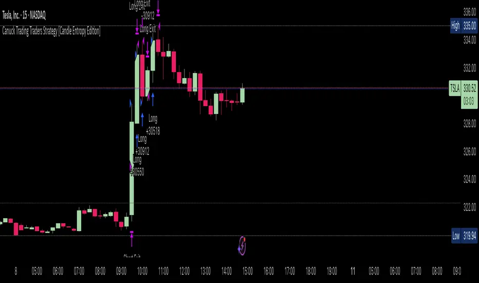
BTC Markup/Markdown Zones by Koenigsegg📈 BTC Markup/Markdown Zones
A handcrafted indicator designed to mark Bitcoin's most critical High Time Frame (HTF) structure shifts. This tool overlays true institutional-level Markup and Markdown Zones, selected manually after deep market review. Whether you're testing strategies or actively trading, this tool gives you the bigger picture at all times.
🔍 Key Features:
✅ HTF Markup & Markdown Zones
Every zone is manually selected — no indicators, no repainting. Just raw market history and real structure.
✅ Two Display Modes
• Background Zones — soft overlays with low opacity for visual context — with the option to increase opacity manually if desired.
• Start Candle Highlight — sharply highlighted candle marking the final pivot before a macro reversal.
✅ Custom Color Controls (Style Tab)
All visual styling lives in the Style tab, with clearly labeled fields:
• Markup Zone
• Markdown Zone
• Start Candle Highlight Markup
• Start Candle Highlight Markdown
✅ Minimal Input Section
Just one toggle: display mode. Everything else is kept clean and intuitive.
🧠 Purpose:
This script is made for any timeframe:
• Zoom into lower timeframes to know whether you're trading inside a Markup or Markdown
• Use it during strategy testing for true structural awareness
📅 Handpicked Macro Turning Points:
Each zone originates from a manually confirmed candle — the last meaningful candle before a shift in control between bulls and bears:
• FRI 19 AUG 2011 12PM – MARK DOWN
• THU 20 OCT 2011 12AM – MARK UP
• WED 10 APR 2013 12PM – MARK DOWN
• FRI 12 APR 2013 12PM – MARK UP
• SAT 30 NOV 2013 12AM – MARK DOWN
• WED 14 JAN 2015 12PM – MARK UP
• SUN 17 DEC 2017 12PM – MARK DOWN
• SAT 15 DEC 2018 12PM – MARK UP
• WED 14 APR 2021 4AM – MARK DOWN
• TUE 22 JUN 2021 12PM – MARK UP
• WED 10 NOV 2021 12PM – MARK DOWN
• MON 21 NOV 2022 8PM – MARK UP
• THU 14 MAR 2024 4AM – MARK DOWN
• MON 5 AUG 2024 12PM – MARK UP
• MON 20 JAN 2025 4AM – MARK DOWN
💡 Zones are manually updated by me after each new confirmed Markup or Markdown.
🧬 Fractal Structure for MTF Systems
Price is fractal — meaning the same principles of structure repeat across all timeframes. In Version 2, this tool evolves by introducing manually selected sub-zones inside each High Time Frame (HTF) Markup or Markdown. These sub-zones reflect Medium Timeframe (MTF) structure shifts, offering precision for traders who operate on both intraday and swing levels.
This makes the indicator ideal for low timeframe (LTF) Markup/Markdown awareness — whether you're managing 15m entries or building multi-timeframe confluence systems.
No auto-zones. No guesswork. Just clean, intentional structure division within the broader trend, handpicked for maximum clarity and edge.
💡 Pro Tip:
When price is inside a Markup Zone, shorting becomes riskier — you're trading against a macro bullish structure.
When inside a Markdown Zone, longing becomes riskier — you're fighting against confirmed bearish momentum.
Use this tool to stay aligned with the broader move, especially when zoomed into smaller timeframes or managing entries/exits during intraday setups.
📈 Markup Phase – Bullish Sentiment
Definition: A period where price makes higher highs and higher lows — the uptrend is in full force.
Why sentiment is bullish:
- Institutions and smart money are already positioned long.
- Public/institutional demand drives prices up.
- Momentum is supported by positive news, breakouts, and FOMO.
- Higher highs confirm buyers are in control.
📉 Markdown Phase – Bearish Sentiment
Definition: A period where price makes lower lows and lower highs — clear downtrend.
Why sentiment is bearish:
- Distribution has already occurred, and supply outweighs demand.
- Smart money is short or sidelined, waiting for deeper prices.
- Panic selling or trend-following traders add downside momentum.
- Lower lows confirm sellers are in control.
❌ Trading Against the Trend — Consequences:
-Reduced Probability of Success
-You’re fighting the dominant flow. Most participants are pushing in the opposite direction.
-Drawdowns & Stop-Outs
-Countertrend trades often get wicked or flushed before any meaningful move, especially without structure-based entries.
-Low Risk-Reward Ratio
-Trends offer sustained moves. Countertrend trades may have small take-profit zones or chop.
-Mental Drain & Doubt
-Fighting momentum causes anxiety, second-guessing, and emotional reactions.
-Missed Opportunities
-Focusing on fighting the trend makes you blind to the high-probability setups with the trend.
-Increased Transaction Costs
-More stop-outs and re-entries mean more fees, more friction.
-FOMO from Watching the Trend Run
-Entering countertrend means you might watch the trend explode without you.
-Confirmation Bias & Stubbornness
-Countertrend traders often look for reasons to justify staying in the wrong direction — leading to bigger losses.
🧠 Summary
In markup = bulls dominate → you swim with the current.
In markdown = bears dominate → going long is like pushing a rock uphill.
Trading with the trend is not just safer, it's smarter. The edge lives in momentum — not ego.
⚠️ Disclaimer
This indicator is for educational and analytical use only. It is not financial advice and should not be relied on for decision-making without personal analysis.
This is not a predictive tool. No indicator can forecast upcoming price movements.
What you see here is based purely on past market behavior — specifically, historical tops and bottoms that marked the start of confirmed reversals.
This script does not know where the next reversal begins, nor can it determine where a new Markup or Markdown starts or ends. It is designed to provide context, not prediction.
Always trade with responsibility and perform your own due diligence.
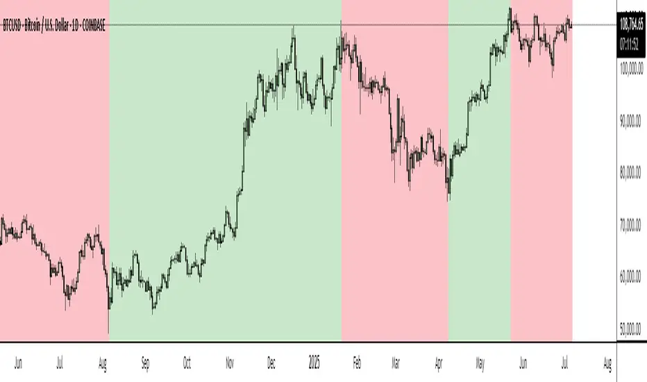
(US) Historical Trade WarsHistorical U.S. Trade Wars Indicator
Overview
This indicator visualizes major U.S. trade wars and disputes throughout modern economic history, from the McKinley Tariff of 1890 to recent U.S.-China tensions. This U.S.-focused timeline is perfect for macro traders, economic historians, and anyone looking to understand how America's trade conflicts correlate with market movements.
Features
Comprehensive U.S. Timeline: Covers 130+ years of U.S.-centered trade disputes with historically accurate dates.
Color-Coded Events:
🔴 Red: Marks the beginning of a U.S. trade war or major dispute.
🟡 Yellow: Highlights significant events within a trade conflict.
🟢 Green: Shows resolutions or ends of trade disputes.
Global Partners/Rivals: Tracks U.S. trade relations with China, Japan, EU, Canada, Mexico, Brazil, Argentina, and others.
Country Flags: Uses emoji flags for easy visual identification of nations in trade relations with the U.S.
Major Trade Wars Covered:
McKinley Tariff (1890-1894)
Smoot-Hawley Tariff Act (1930-1934)
U.S.-Europe Chicken War (1962-1974)
Multifiber Arrangement Quotas (1974-2005)
Japan-U.S. Trade Disputes (1981-1989)
NAFTA and Softwood Lumber Disputes
Clinton and Bush-Era Steel Tariffs
Obama-Era China Tire Tariffs
Rare Earth Minerals Dispute (2012-2014)
Solar Panel Dispute (2012-2015)
TPP and TTIP Negotiations
U.S.-China Trade War (2018-present)
Airbus-Boeing Dispute
Usage
Analyze how markets historically responded to trade war initiations and resolutions.
Identify patterns in market behavior during periods of trade tensions.
Use as an overlay with price action to examine correlations.
Perfect companion for macro analysis on daily, weekly, or monthly charts.
About
This indicator is designed as a historical reference tool for traders and economic analysts focusing on U.S. trade policy and its global impact. The dates and events have been thoroughly researched for accuracy. Each label includes emojis to indicate the U.S. and its trade partners/rivals, making it easy to track America's evolving trade relationships across time.
Note: This indicator works best on larger timeframes (daily, weekly, monthly) due to the historical span covered.

[blackcat] L2 Kiosotto IndicatorOVERVIEW
The Kiosotto Indicator is a versatile technical analysis tool designed for forex trading but applicable to other financial markets. It excels in detecting market reversals and trends without repainting, ensuring consistent and reliable signals. The indicator has evolved over time, with different versions focusing on specific aspects of market analysis.
KEY FEATURES
Reversal Detection: Identifies potential market reversals, crucial for traders looking to capitalize on turning points.
Trend Detection: Earlier versions focused on detecting trends, useful for traders who prefer to follow the market direction.
Non-Repainting: Signals remain consistent on the chart, providing reliable and consistent signals.
Normalization: Later versions, such as Normalized Kiosotto and Kiosotto_2025, incorporate normalization to assess oversold and overbought conditions, enhancing interpretability.
VERSIONS AND EVOLUTION
Early Versions: Focused on trend detection, useful for following market direction.
2 in 1 Kiosotto: Emphasizes reversal detection and is considered an improvement by users.
Normalized Versions (e.g., Kiosotto_2025, Kiosotto_3_2025): Introduce normalization to assess oversold and overbought conditions, enhancing interpretability.
HOW TO USE THE KIOSOTTO INDICATOR
Understanding Signals:
Reversals: Look for the indicator's signals that suggest a potential reversal, indicated by color changes, line crossings, or other visual cues.
Trends: Earlier versions might show stronger trending signals, indicated by the direction or slope of the indicator's lines.
Normalization Interpretation (for normalized versions):
Oversold: When the indicator hits the lower boundary, it might indicate an oversold condition, suggesting a potential buy signal.
Overbought: Hitting the upper boundary could signal an overbought condition, suggesting a potential sell signal.
PINE SCRIPT IMPLEMENTATION
The provided Pine Script code is a version of the Kiosotto indicator. Here's a detailed explanation of the code:
//@version=5
indicator(" L2 Kiosotto Indicator", overlay=false)
//Pine version of Kiosotto 2015 v4 Alert ms-nrp
// Input parameters
dev_period = input.int(150, "Dev Period")
alerts_level = input.float(15, "Alerts Level")
tsbul = 0.0
tsber = 0.0
hpres = 0.0
lpres = 9999999.0
for i = 0 to dev_period - 1
rsi = ta.rsi(close , dev_period)
if high > hpres
hpres := high
tsbul := tsbul + rsi * close
if low < lpres
lpres := low
tsber := tsber + rsi * close
buffer1 = tsber != 0 ? tsbul / tsber : 0
buffer2 = tsbul != 0 ? tsber / tsbul : 0
// Plotting
plot(buffer1, color=color.aqua, linewidth=3, style=plot.style_histogram)
plot(buffer2, color=color.fuchsia, linewidth=3, style=plot.style_histogram)
hline(alerts_level, color=color.silver)
EXPLANATION OF THE CODE
Indicator Definition:
indicator(" L2 Kiosotto Indicator", overlay=false): Defines the indicator with the name " L2 Kiosotto Indicator" and specifies that it should not be overlaid on the price chart.
Input Parameters:
dev_period = input.int(150, "Dev Period"): Allows users to set the period for the deviation calculation.
alerts_level = input.float(15, "Alerts Level"): Allows users to set the level for alerts.
Initialization:
tsbul = 0.0: Initializes the tsbul variable to 0.0.
tsber = 0.0: Initializes the tsber variable to 0.0.
hpres = 0.0: Initializes the hpres variable to 0.0.
lpres = 9999999.0: Initializes the lpres variable to a very high value.
Loop for Calculation:
The for loop iterates over the last dev_period bars.
rsi = ta.rsi(close , dev_period): Calculates the RSI for the current bar.
if high > hpres: If the high price of the current bar is greater than hpres, update hpres and add the product of RSI and close price to tsbul.
if low < lpres: If the low price of the current bar is less than lpres, update lpres and add the product of RSI and close price to tsber.
Buffer Calculation:
buffer1 = tsber != 0 ? tsbul / tsber : 0: Calculates the first buffer as the ratio of tsbul to tsber if tsber is not zero.
buffer2 = tsbul != 0 ? tsber / tsbul : 0: Calculates the second buffer as the ratio of tsber to tsbul if tsbul is not zero.
Plotting:
plot(buffer1, color=color.aqua, linewidth=3, style=plot.style_histogram): Plots the first buffer as a histogram with an aqua color.
plot(buffer2, color=color.fuchsia, linewidth=3, style=plot.style_histogram): Plots the second buffer as a histogram with a fuchsia color.
hline(alerts_level, color=color.silver): Draws a horizontal line at the alerts_level with a silver color.
FUNCTIONALITY
The Kiosotto indicator calculates two buffers based on the RSI and price levels over a specified period. The buffers are plotted as histograms, and a horizontal line is drawn at the alerts level. The indicator helps traders identify potential reversals and trends by analyzing the relationship between the RSI and price levels.
ALGORITHMS
RSI Calculation:
The Relative Strength Index (RSI) measures the speed and change of price movements. It is calculated using the formula:
RSI=100− (1+RS) / 100
where RS is the ratio of the average gain to the average loss over the specified period.
Buffer Calculation:
The buffers are calculated as the ratio of the sum of RSI multiplied by the close price for high and low price conditions. This helps in identifying the balance between buying and selling pressure.
Signal Generation:
The indicator generates signals based on the values of the buffers and the alerts level. Traders can use these signals to make informed trading decisions, such as entering or exiting trades based on potential reversals or trends.
APPLICATION SCENARIOS
Reversal Trading: Traders can use the Kiosotto indicator to identify potential reversals by looking for significant changes in the buffer values or crossings of the alerts level.
Trend Following: The indicator can also be used to follow trends by analyzing the direction and slope of the buffer lines.
Oversold/Overbought Conditions: For normalized versions, traders can use the indicator to identify oversold and overbought conditions, which can provide buy or sell signals.
THANKS
Special thanks to the TradingView community and the original developers for their contributions and support in creating and refining the Kiosotto Indicator.
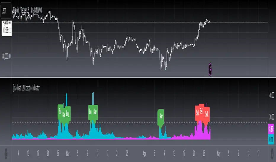
4-Year Cycles [jpkxyz]Overview of the Script
I wanted to write a script that encompasses the wide-spread macro fund manager investment thesis: "Crypto is simply and expression of macro." A thesis pioneered by the likes of Raoul Pal (EXPAAM) , Andreesen Horowitz (A16Z) , Joe McCann (ASYMETRIC) , Bob Loukas and many more.
Cycle Theory Background:
The 2007-2008 financial crisis transformed central bank monetary policy by introducing:
- Quantitative Easing (QE): Creating money to buy assets and inject liquidity
- Coordinated global monetary interventions
Proactive 4-year economic cycles characterised by:
- Expansionary periods (low rates, money creation)
- Followed by contraction/normalisation
Central banks now deliberately manipulate liquidity, interest rates, and asset prices to control economic cycles, using monetary policy as a precision tool rather than a blunt instrument.
Cycle Characteristics (based on historical cycles):
- A cycle has 4 seasons (Spring, Summer, Fall, Winter)
- Each season with a cycle lasts 365 days
- The Cycle Low happens towards the beginning of the Spring Season of each new cycle
- This is followed by a run up throughout the Spring and Summer Season
- The Cycle High happens towards the end of the Fall Season
- The Winter season is characterised by price corrections until establishing a new floor in the Spring of the next cycle
Key Functionalities
1. Cycle Tracking
- Divides market history into 4-year cycles (Spring, Summer, Fall, Winter)
- Starts tracking cycles from 2011 (first cycle after the 2007 crisis cycle)
- Identifies and marks cycle boundaries
2. Visualization
- Colors background based on current cycle season
- Draws lines connecting:
- Cycle highs and lows
- Inter-cycle price movements
- Adds labels showing:
- Percentage gains/losses between cycles
- Number of days between significant points
3. Customization Options
- Allows users to customize:
- Colors for each season
- Line and label colors
- Label size
- Background opacity
Detailed Mechanism
Cycle Identification
- Uses a modulo calculation to determine the current season in the 4-year cycle
- Preset boundary years include 2015, 2019, 2023, 2027
- Automatically tracks and marks cycle transitions
Price Analysis
- Tracks highest and lowest prices within each cycle
- Calculates percentage changes:
- Intra-cycle (low to high)
- Inter-cycle (previous high to current high/low)
Visualization Techniques
- Background color changes based on current cycle season
- Dashed and solid lines connect significant price points
- Labels provide quantitative insights about price movements
Unique Aspects
1. Predictive Cycle Framework: Provides a structured way to view market movements beyond traditional technical analysis
2. Seasonal Color Coding: Intuitive visual representation of market cycle stages
3. Comprehensive Price Tracking: Captures both intra-cycle and inter-cycle price dynamics
4. Highly Customizable: Users can adjust visual parameters to suit their preferences
Potential Use Cases
- Technical analysis for long-term investors
- Identifying market cycle patterns
- Understanding historical price movement rhythms
- Educational tool for market cycle theory
Limitations/Considerations
- Based on a predefined 4-year cycle model (Liquidity Cycles)
- Historic Cycle Structures are not an indication for future performance
- May not perfectly represent all market behavior
- Requires visual interpretation
This script is particularly interesting for investors who believe in cyclical market theories and want a visual, data-driven representation of market stages.

MicuRobert EMA Cross StrategyThis is a repost of a old strategy that cant be updated anymore, it was a request for a user made in Oct, 6, 2015
Here's a possible engaging description for the tradingview script:
**MicuRobert EMA Cross V2: A Powerful Trading Strategy**
Join the ranks of successful traders with this advanced strategy, designed to help you profit from market trends. The MicuRobert EMA Cross V2 combines two essential indicators - Exponential Moving Average (EMA) and Divergence EMA (DEMA) - to generate buy and sell signals.
**Key Features:**
* **Trading Session Filter**: Only trade during your preferred session, ensuring you're in sync with market conditions.
* **Trailing Stop**: Automatically adjust stop-loss levels to lock in profits or limit losses.
* **Customizable Trade Size**: Set the size of each trade based on your risk tolerance and trading goals.
**How it Works:**
The script uses two EMAs (5-period and 34-period) to identify trends. When the shorter EMA crosses above the longer one, a buy signal is generated. Conversely, when the shorter EMA falls below the longer one, a sell signal is triggered. The strategy also incorporates divergence analysis between price action and the EMAs.
**Visual Aids:**
* **EMA Plots**: Visualize the two EMAs on your chart to gauge market momentum.
* **Buy/Sell Signals**: See when buy or sell signals are generated, along with their corresponding entry prices.
* **Trailing Stop Lines**: Monitor stop-loss levels as they adjust based on price action.
**Get Started:**
Download this script and start trading like a pro! With its robust features and customizable settings, the MicuRobert EMA Cross V2 is an excellent addition to any trader's arsenal.
~Llama3

McRib Bull Market Indicator# McRib Bull Market Indicator
## Overview
The McRib Bull Market Indicator is a unique technical analysis tool that marks McDonald's McRib sandwich release dates on your trading charts. While seemingly unconventional, this indicator serves as a fascinating historical reference point for market analysis, particularly for studying periods of market expansion.
## Key Features
- Visual yellow labels marking verified McRib release dates from 2012 to 2024
- Clean, unobtrusive design that overlays on any chart timeframe
- Covers both U.S. and international releases (including UK and Australia)
## Historical Reference Points
The indicator includes release dates from:
- December 2012
- October-December 2014
- January 2015
- October 2016
- November 2017
- October 2018
- October 2019
- December 2020
- October 2022
- November 2023
- December 2024
## Usage Guide
1. Add the indicator to any chart by searching for "McRib Bull Market Indicator"
2. The indicator will automatically display yellow labels above price candles on McRib release dates
3. Use these reference points to:
- Analyze market conditions during McRib releases
- Study potential correlations between releases and market movements
- Compare market behavior across different McRib release periods
- Identify any patterns in market expansion phases coinciding with releases
## Trading Application
While initially created as a novelty indicator, it can be used to:
- Mark specific historical points of reference for broader market analysis
- Study potential market psychology around major promotional events
- Compare seasonal market patterns with recurring release dates
- Analyze market expansion phases that coincide with releases
Remember: While this indicator provides interesting historical reference points, it should be used as part of a comprehensive trading strategy rather than as a standalone trading signal.
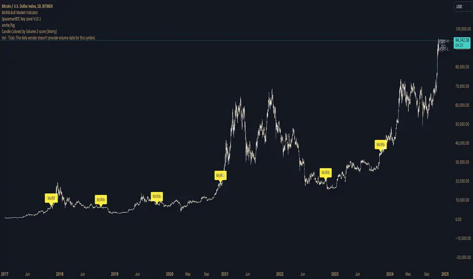
Economic Policy Uncertainty StrategyThis Pine Script strategy is designed to make trading decisions based on the Economic Policy Uncertainty Index for the United States (USEPUINDXD) using a Simple Moving Average (SMA) and a dynamic threshold. The strategy identifies opportunities by entering long positions when the SMA of the Economic Policy Uncertainty Index crosses above a user-defined threshold. An exit is triggered after a set number of bars have passed since the trade was opened. Additionally, the background is highlighted in green when a position is open to visually indicate active trades.
This strategy is intended to be used in portfolio management and trading systems where economic policy uncertainty plays a critical role in decision-making. The index provides insight into macroeconomic conditions, which can affect asset prices and investment returns.
The Economic Policy Uncertainty (EPU) Index is a significant metric used to gauge uncertainty related to economic policies in the United States. This index reflects the frequency of newspaper articles discussing economic uncertainty, government policies, and their potential impact on the economy. It has become a popular indicator for both academics and practitioners to analyze the effects of policy uncertainty on various economic and financial outcomes.
Importance of the EPU Index for Portfolio Decisions:
Economic Policy Uncertainty and Investment Decisions:
Research by Baker, Bloom, and Davis (2016) introduced the Economic Policy Uncertainty Index and explored how increased uncertainty leads to delays in investment and hiring decisions. Their study shows that heightened uncertainty, as captured by the EPU index, is associated with a contraction in economic activity and lower stock market returns. Investors tend to shift their portfolios towards safer assets during periods of high policy uncertainty .
Impact on Asset Prices:
Gulen and Ion (2016) demonstrated that policy uncertainty adversely affects corporate investment, leading to lower stock market returns. The study emphasized that firms reduce investment during periods of high policy uncertainty, which can significantly impact the pricing of risky assets. Consequently, portfolio managers need to account for policy uncertainty when making asset allocation decisions .
Global Implications:
Policy uncertainty is not only a domestic issue. Brogaard and Detzel (2015) found that U.S. economic policy uncertainty has significant spillover effects on global financial markets, affecting equity returns, bond yields, and foreign exchange rates. This suggests that global investors should incorporate U.S. policy uncertainty into their risk management strategies .
These studies underscore the importance of the Economic Policy Uncertainty Index as a tool for understanding macroeconomic risks and making informed portfolio management decisions. Strategies that incorporate the EPU index, such as the one described above, can help investors navigate periods of uncertainty by adjusting their exposure to different asset classes based on economic conditions.
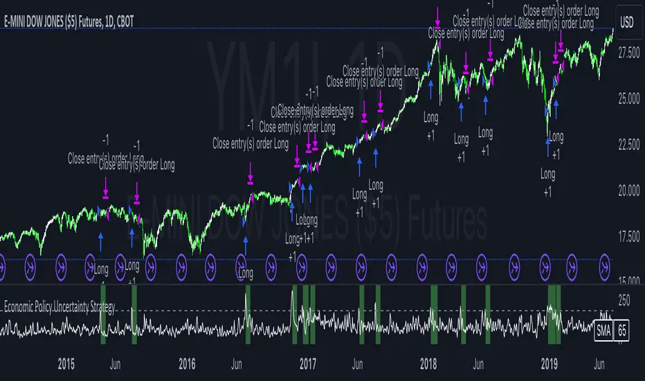
Dual Chain StrategyDual Chain Strategy - Technical Overview
How It Works:
The Dual Chain Strategy is a unique approach to trading that utilizes Exponential Moving Averages (EMAs) across different timeframes, creating two distinct "chains" of trading signals. These chains can work independently or together, capturing both long-term trends and short-term price movements.
Chain 1 (Longer-Term Focus):
Entry Signal: The entry signal for Chain 1 is generated when the closing price crosses above the EMA calculated on a weekly timeframe. This suggests the start of a bullish trend and prompts a long position.
bullishChain1 = enableChain1 and ta.crossover(src1, entryEMA1)
Exit Signal: The exit signal is triggered when the closing price crosses below the EMA on a daily timeframe, indicating a potential bearish reversal.
exitLongChain1 = enableChain1 and ta.crossunder(src1, exitEMA1)
Parameters: Chain 1's EMA length is set to 10 periods by default, with the flexibility for user adjustment to match various trading scenarios.
Chain 2 (Shorter-Term Focus):
Entry Signal: Chain 2 generates an entry signal when the closing price crosses above the EMA on a 12-hour timeframe. This setup is designed to capture quicker, shorter-term movements.
bullishChain2 = enableChain2 and ta.crossover(src2, entryEMA2)
Exit Signal: The exit signal occurs when the closing price falls below the EMA on a 9-hour timeframe, indicating the end of the shorter-term trend.
exitLongChain2 = enableChain2 and ta.crossunder(src2, exitEMA2)
Parameters: Chain 2's EMA length is set to 9 periods by default, and can be customized to better align with specific market conditions or trading strategies.
Key Features:
Dual EMA Chains: The strategy's originality shines through its dual-chain configuration, allowing traders to monitor and react to both long-term and short-term market trends. This approach is particularly powerful as it combines the strengths of trend-following with the agility of momentum trading.
Timeframe Flexibility: Users can modify the timeframes for both chains, ensuring the strategy can be tailored to different market conditions and individual trading styles. This flexibility makes it versatile for various assets and trading environments.
Independent Trade Logic: Each chain operates independently, with its own set of entry and exit rules. This allows for simultaneous or separate execution of trades based on the signals from either or both chains, providing a robust trading system that can handle different market phases.
Backtesting Period: The strategy includes a configurable backtesting period, enabling thorough performance assessment over a historical range. This feature is crucial for understanding how the strategy would have performed under different market conditions.
time_cond = time >= startDate and time <= finishDate
What It Does:
The Dual Chain Strategy offers traders a distinctive trading tool that merges two separate EMA-based systems into one cohesive framework. By integrating both long-term and short-term perspectives, the strategy enhances the ability to adapt to changing market conditions. The originality of this script lies in its innovative dual-chain design, providing traders with a unique edge by allowing them to capitalize on both significant trends and smaller, faster price movements.
Whether you aim to capture extended market trends or take advantage of more immediate price action, the Dual Chain Strategy provides a comprehensive solution with a high degree of customization and strategic depth. Its flexibility and originality make it a valuable tool for traders seeking to refine their approach to market analysis and execution.
How to Use the Dual Chain Strategy
Step 1: Access the Strategy
Add the Script: Start by adding the Dual Chain Strategy to your TradingView chart. You can do this by searching for the script by name or using the link provided.
Select the Asset: Apply the strategy to your preferred trading pair or asset, such as #BTCUSD, to see how it performs.
Step 2: Configure the Settings
Enable/Disable Chains:
The strategy is designed with two independent chains. You can choose to enable or disable each chain depending on your trading style and the market conditions.
enableChain1 = input.bool(true, title='Enable Chain 1')
enableChain2 = input.bool(true, title='Enable Chain 2')
By default, both chains are enabled. If you prefer to focus only on longer-term trends, you might disable Chain 2, or vice versa if you prefer shorter-term trades.
Set EMA Lengths:
Adjust the EMA lengths for each chain to match your trading preferences.
Chain 1: The default EMA length is 10 periods. This chain uses a weekly timeframe for entry signals and a daily timeframe for exits.
len1 = input.int(10, minval=1, title='Length Chain 1 EMA', group="Chain 1")
Chain 2: The default EMA length is 9 periods. This chain uses a 12-hour timeframe for entries and a 9-hour timeframe for exits.
len2 = input.int(9, minval=1, title='Length Chain 2 EMA', group="Chain 2")
Customize Timeframes:
You can customize the timeframes used for entry and exit signals for both chains.
Chain 1:
Entry Timeframe: Weekly
Exit Timeframe: Daily
tf1_entry = input.timeframe("W", title='Chain 1 Entry Timeframe', group="Chain 1")
tf1_exit = input.timeframe("D", title='Chain 1 Exit Timeframe', group="Chain 1")
Chain 2:
Entry Timeframe: 12 Hours
Exit Timeframe: 9 Hours
tf2_entry = input.timeframe("720", title='Chain 2 Entry Timeframe (12H)', group="Chain 2")
tf2_exit = input.timeframe("540", title='Chain 2 Exit Timeframe (9H)', group="Chain 2")
Set the Backtesting Period:
Define the period over which you want to backtest the strategy. This allows you to see how the strategy would have performed historically.
startDate = input.time(timestamp('2015-07-27'), title="StartDate")
finishDate = input.time(timestamp('2026-01-01'), title="FinishDate")
Step 3: Analyze the Signals
Understand the Entry and Exit Signals:
Buy Signals: When the price crosses above the entry EMA, the strategy generates a buy signal.
bullishChain1 = enableChain1 and ta.crossover(src1, entryEMA1)
Sell Signals: When the price crosses below the exit EMA, the strategy generates a sell signal.
bearishChain2 = enableChain2 and ta.crossunder(src2, entryEMA2)
Review the Visual Indicators:
The strategy plots buy and sell signals on the chart with labels for easy identification:
BUY C1/C2 for buy signals from Chain 1 and Chain 2.
SELL C1/C2 for sell signals from Chain 1 and Chain 2.
This visual aid helps you quickly understand when and why trades are being executed.
Step 4: Optimize the Strategy
Backtest Results:
Review the strategy’s performance over the backtesting period. Look at key metrics like net profit, drawdown, and trade statistics to evaluate its effectiveness.
Adjust the EMA lengths, timeframes, and other settings to see how changes affect the strategy’s performance.
Customize for Live Trading:
Once satisfied with the backtest results, you can apply the strategy settings to live trading. Remember to continuously monitor and adjust as needed based on market conditions.
Step 5: Implement Risk Management
Use Realistic Position Sizing:
Keep your risk exposure per trade within a comfortable range, typically between 1-2% of your trading capital.
Set Alerts:
Set up alerts for buy and sell signals, so you don’t miss trading opportunities.
Paper Trade First:
Consider running the strategy in a paper trading account to understand its behavior in real market conditions before committing real capital.
This dual-layered approach offers a distinct advantage: it enables the strategy to adapt to varying market conditions by capturing both broad trends and immediate price action without one chain's activity impacting the other's decision-making process. The independence of these chains in executing transactions adds a level of sophistication and flexibility that is rarely seen in more conventional trading systems, making the Dual Chain Strategy not just unique, but a powerful tool for traders seeking to navigate complex market environments.