FlexiMA Variance Tracker [presentTrading]🔶 Introduction and How it is Different
The FlexiMA Variance Tracker (FlexiMA-VT) represents a novel approach in technical analysis, distinctively standing out in the realm of financial market indicators. It leverages the concept of a variable Length Moving Average (MA) to create a versatile and dynamic oscillator. Unlike traditional oscillators that rely on a fixed-length MA, the FlexiMA-VT adapts to market conditions by varying the length of the MA, offering a more responsive and nuanced view of market trends. (*The achieved method took reference from SuperTrend Polyfactor Oscillator)
This innovative design allows the FlexiMA-VT to capture a broader spectrum of market movements, making it highly effective in diverse trading environments. Whether in stable or volatile markets, its adaptability ensures consistent relevance, providing traders with deeper insights into potential market swings.
The proposed oscillator accentuates several key aspects through a distinctive mesh of bars, which are derived from the differences between the price and a set of 20 Moving Averages, each altered by varying factors. The intensity of the mesh's colors serves as an indicator, with brighter hues signifying a greater convergence of Moving Average signals.
Starting Length = 5
Starting Length = 40
🔶 Strategy, How it Works: Detailed Explanation
1. Core Concept:
The FlexiMA-VT operates by comparing the price or an average value (indicator source) against a set of moving averages with varying lengths.
These lengths are dynamically adjusted through a starting factor and multiple increment factors, ensuring a comprehensive analysis over different time scales.
2. Normalization and Standard Deviation Calculation:
Once deviations are calculated, they undergo a normalization process, which can be set to 'None', 'Max-Min', or 'Absolute Sum'.
This step is crucial as it standardizes the deviations, allowing for a consistent scale of comparison.
The standard deviation of these normalized deviations is then calculated, offering insights into the market’s volatility and potential trend strength.
🔹Normalization
3. Median Value and Oscillator Creation:
The median of the normalized deviations forms the core of the FlexiMA-VT oscillator.
This median value provides a balanced central point, reflecting the consensus of various MA lengths.
The standard deviation bands plotted around the median enhance the interpretative power of the oscillator, indicating potential overbought or oversold conditions.
4. Multi-Factor Analysis:
The FlexiMA-VT uses multiple increment factors to generate a range of MAs, each factor representing a different scale of trend analysis.
By averaging the results from these different scales, the FlexiMA-VT forms a more comprehensive and reliable oscillator.
🔹Consensus
5. Practical Application:
Traders can use the FlexiMA-VT for various purposes, including identifying trend reversals, gauging market momentum, and determining overbought or oversold conditions.
Its dynamic nature makes it adaptable to different trading strategies, from short-term scalping to long-term position trading.
🔶 Settings
1. Indicator Source (indicatorSource): Determines the base data for calculations, typically a price average (HLC3).
2. Indicator Length (indicatorLength): Sets the base length for Moving Averages, influencing initial calculations.
3. Starting Factor (startingFactor): Initial multiplier for MA length, impacting the starting point of analysis.
4. Increment Factors (incrementFactor_1, incrementFactor_2, incrementFactor_3): Modulate the rate of change in MA lengths, adding variability.
5. Normalization Method (normalizeMethod): Standardizes deviations, with methods like 'Max-Min' and 'Absolute Sum' for comparability.
Cerca negli script per "indicators"

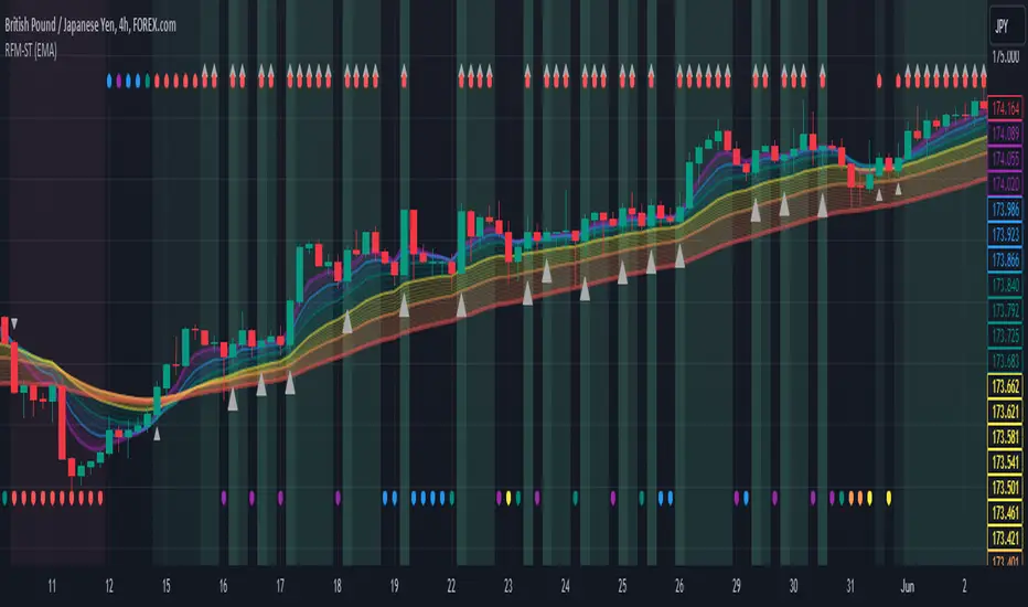
Rainbow Fibonacci Momentum - SuperTrend🌈 "Rainbow Fibonacci Momentum - SuperTrend" Indicator 🌈
IMPORTANT: as this is a complex and elaborate TREND ANALYSIS on the graph, ALL INDICATORS REPAINT.
Experience the brilliance of "Rainbow Fibonacci Momentum - SuperTrend" for your technical analysis on TradingView! This versatile indicator allows you to visualize various types of Moving Averages, including Simple Moving Averages (SMA), Exponential Moving Averages (EMA), Weighted Moving Averages (WMA), Hull Moving Averages (HMA), and Volume Weighted Moving Averages (VWMA).
Each MA displayed in a unique color to create a stunning rainbow effect. This makes it easier for you to identify trends and potential trading opportunities.
Key Features:
📊 Multiple Moving Average Types - Choose from a range of moving average types to suit your analysis.
🎨 Stunning Color Gradient - Each moving average type is displayed in a unique color, creating a beautiful rainbow effect.
📉 Overlay Compatible - Use it as an overlay on your price chart for clear trend insights.
With the "Rainbow Fibonacci Momentum - SuperTrend" indicator, you'll add a burst of color to your trading routine and gain a deeper understanding of market trends.
HOW IT WORKS
MA Lines:
MA - 5: purple lines
MA - 8: blue lines
MA - 13: green lines
MA - 21: yellow lines
MA - 34: orange lines
MA - 55: red line
Header Color Indicators:
Purple: MA-5 is in uptrend on the chart
Blue: MA-5 and MA-8 are in the uptrend on the chart
Green: MA-5, MA-8 and MA-13 are in the uptrend on the chart
Yellow: MA-5, MA-8, MA-13 and MA-21 are in the uptrend on the chart
Orange: MA-5, MA-8, MA-13, MA-21 and MA-34 are in the uptrend on the chart
Red: MA-5, MA-8, MA-13, MA-21, MA-34 and MA-55 are in the uptrend on the chart
Red + White Arrow: All MAs are correctly aligned in the uptrend on the chart
Footer Color Indicators:
Purple: MA-5 is in downtrend on the chart
Blue: MA-5 and MA-8 are in the downtrend on the chart
Green: MA-5, MA-8 and MA-13 are in the downtrend on the chart
Yellow: MA-5, MA-8, MA-13 and MA-21 are in the downtrend on the chart
Orange: MA-5, MA-8, MA-13, MA-21 and MA-34 are in the downtrend on the chart
Red: MA-5, MA-8, MA-13, MA-21, MA-34 and MA-55 are in the downtrend on the chart
Red + White Arrow: All MAs are correctly aligned in the downtrend on the chart
Background Colors:
Light Red: All MAs are on the rise!
Red: All MAs are align correctly on the rise!
Light Green: All MAs are in freefall!
Green: All MAs are align correctly in freefall!
Tiny Arrows Indicators/Alerts:
Down Arrow: All MAs are in freefall!
Up Arrow: All MAs are on the rise!
Big Arrows Indicators/Alerts:
Down Arrow: All MAs are align correctly in freefall!
Up Arrow: All MAs are align correctly on the rise!
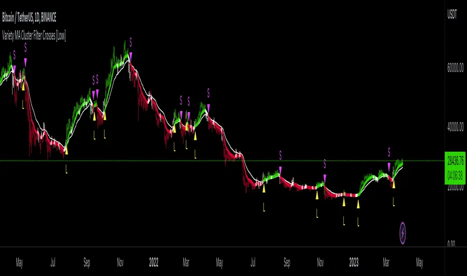
Variety MA Cluster Filter Crosses [Loxx]What is a Cluster Filter?
One of the approaches to determining a useful signal (trend) in stream data. Small filtering (smoothing) tests applied to market quotes demonstrate the potential for creating non-lagging digital filters (indicators) that are not redrawn on the last bars.
Standard Approach
This approach is based on classical time series smoothing methods. There are lots of articles devoted to this subject both on this and other websites. The results are also classical:
1. The changes in trends are displayed with latency;
2. Better indicator (digital filter) response achieved at the expense of smoothing quality decrease;
3. Attempts to implement non-lagging indicators lead to redrawing on the last samples (bars).
And whereas traders have learned to cope with these things using persistence of economic processes and other tricks, this would be unacceptable in evaluating real-time experimental data, e.g. when testing aerostructures.
The Main Problem
It is a known fact that the majority of trading systems stop performing with the course of time, and that the indicators are only indicative over certain intervals. This can easily be explained: market quotes are not stationary. The definition of a stationary process is available in Wikipedia:
A stationary process is a stochastic process whose joint probability distribution does not change when shifted in time.
Judging by this definition, methods of analysis of stationary time series are not applicable in technical analysis. And this is understandable. A skillful market-maker entering the market will mess up all the calculations we may have made prior to that with regard to parameters of a known series of market quotes.
Even though this seems obvious, a lot of indicators are based on the theory of stationary time series analysis. Examples of such indicators are moving averages and their modifications. However, there are some attempts to create adaptive indicators. They are supposed to take into account non-stationarity of market quotes to some extent, yet they do not seem to work wonders. The attempts to "punish" the market-maker using the currently known methods of analysis of non-stationary series (wavelets, empirical modes and others) are not successful either. It looks like a certain key factor is constantly being ignored or unidentified.
The main reason for this is that the methods used are not designed for working with stream data. All (or almost all) of them were developed for analysis of the already known or, speaking in terms of technical analysis, historical data. These methods are convenient, e.g., in geophysics: you feel the earthquake, get a seismogram and then analyze it for few months. In other words, these methods are appropriate where uncertainties arising at the ends of a time series in the course of filtering affect the end result.
When analyzing experimental stream data or market quotes, we are focused on the most recent data received, rather than history. These are data that cannot be dealt with using classical algorithms.
Cluster Filter
Cluster filter is a set of digital filters approximating the initial sequence. Cluster filters should not be confused with cluster indicators.
Cluster filters are convenient when analyzing non-stationary time series in real time, in other words, stream data. It means that these filters are of principal interest not for smoothing the already known time series values, but for getting the most probable smoothed values of the new data received in real time.
Unlike various decomposition methods or simply filters of desired frequency, cluster filters create a composition or a fan of probable values of initial series which are further analyzed for approximation of the initial sequence. The input sequence acts more as a reference than the target of the analysis. The main analysis concerns values calculated by a set of filters after processing the data received.
In the general case, every filter included in the cluster has its own individual characteristics and is not related to others in any way. These filters are sometimes customized for the analysis of a stationary time series of their own which describes individual properties of the initial non-stationary time series. In the simplest case, if the initial non-stationary series changes its parameters, the filters "switch" over. Thus, a cluster filter tracks real time changes in characteristics.
Cluster Filter Design Procedure
Any cluster filter can be designed in three steps:
1. The first step is usually the most difficult one but this is where probabilistic models of stream data received are formed. The number of these models can be arbitrary large. They are not always related to physical processes that affect the approximable data. The more precisely models describe the approximable sequence, the higher the probability to get a non-lagging cluster filter.
2. At the second step, one or more digital filters are created for each model. The most general condition for joining filters together in a cluster is that they belong to the models describing the approximable sequence.
3. So, we can have one or more filters in a cluster. Consequently, with each new sample we have the sample value and one or more filter values. Thus, with each sample we have a vector or artificial noise made up of several (minimum two) values. All we need to do now is to select the most appropriate value.
An Example of a Simple Cluster Filter
For illustration, we will implement a simple cluster filter corresponding to the above diagram, using market quotes as input sequence. You can simply use closing prices of any time frame.
1. Model description. We will proceed on the assumption that:
The aproximate sequence is non-stationary, i.e. its characteristics tend to change with the course of time.
The closing price of a bar is not the actual bar price. In other words, the registered closing price of a bar is one of the noise movements, like other price movements on that bar.
The actual price or the actual value of the approximable sequence is between the closing price of the current bar and the closing price of the previous bar.
The approximable sequence tends to maintain its direction. That is, if it was growing on the previous bar, it will tend to keep on growing on the current bar.
2. Selecting digital filters. For the sake of simplicity, we take two filters:
The first filter will be a variety filter calculated based on the last closing prices using the slow period. I believe this fits well in the third assumption we specified for our model.
Since we have a non-stationary filter, we will try to also use an additional filter that will hopefully facilitate to identify changes in characteristics of the time series. I've chosen a variety filter using the fast period.
3. Selecting the appropriate value for the cluster filter.
So, with each new sample we will have the sample value (closing price), as well as the value of MA and fast filter. The closing price will be ignored according to the second assumption specified for our model. Further, we select the МА or ЕМА value based on the last assumption, i.e. maintaining trend direction:
For an uptrend, i.e. CF(i-1)>CF(i-2), we select one of the following four variants:
if CF(i-1)fastfilter(i), then CF(i)=slowfilter(i);
if CF(i-1)>slowfilter(i) and CF(i-1)slowfilter(i) and CF(i-1)>fastfilter(i), then CF(i)=MAX(slowfilter(i),fastfilter(i)).
For a downtrend, i.e. CF(i-1)slowfilter(i) and CF(i-1)>fastfilter(i), then CF(i)=MAX(slowfilter(i),fastfilter(i));
if CF(i-1)>slowfilter(i) and CF(i-1)fastfilter(i), then CF(i)=fastfilter(i);
if CF(i-1)
Wavetrend in Dynamic Zones with Kumo Implied VolatilityI was asked to do one of those, so here we go...
As always free and open source as it should be. Do not pay for such indicators!
A WaveTrend Indicator or also widely known as "Market Cipher" is an Indicator that is based on Moving Averages, therefore its an "lagging indicator". Lagging indicators are best used in combination with leading indicators. In this script the "leading indicator" component are Daily, Weekly or Monthly Pivots . These Pivots can be used as dynamic Support and Resistance , Stoploss, Take Profit etc.
This indicator combination is best used in larger timeframes. For lower timeframes you might need to change settings to your liking.
The general Wavetrend settings are the same that are used in Market Cipher, Market Liberator and such popular indicators.
What are these circles?
-These are the WaveTrend Divergences. Red for Regular-Bearish. Orange for Hidden-Bearish. Green for Regular-Bullish. Aqua for Hidden-Bullish.
What are these white, orange and aqua triangles?
-These are the WaveTrend Pivots. A Pivot counter was added. Every time a pivot is lower than the previous one, an orange triangle is printed, every time a pivot is higher than the previous one an aqua triangle is printed. That mimics a very common way Wavetrend is being used for trading when using those other paid Wavetrend indicators.
What are these Orange and Aqua Zones?
-These are Dynamic Zones based on the indicator itself, they offer more information than static zones. Of course static lines are also included and can be adjusted.
What are the lines between the waves?
-This is a Kumo Cloud Implied Volatility indicator. It is color coded and can be used to indicate if a major market move/bottom/top happened.
What are those numbers on the right?
-The first number is a Bollinger Band indicator that shows if said Bollinger Band is in a state of Oversold/Overbought, the second number is the actual Bollinger Band Width that indicates if the Bollinger Band squeezes, normally that happens right before the market makes an explosive move.
Please keep in mind that this indicator is a tool and not a strategy, do not blindly trade signals, do your own research first! Use this indicator in conjunction with other indicators to get multiple confirmations.

Ehlers Autocorrelation Periodogram [Loxx]Ehlers Autocorrelation Periodogram contains two versions of Ehlers Autocorrelation Periodogram Algorithm. This indicator is meant to supplement adaptive cycle indicators that myself and others have published on Trading View, will continue to publish on Trading View. These are fast-loading, low-overhead, streamlined, exact replicas of Ehlers' work without any other adjustments or inputs.
Versions:
- 2013, Cycle Analytics for Traders Advanced Technical Trading Concepts by John F. Ehlers
- 2016, TASC September, "Measuring Market Cycles"
Description
The Ehlers Autocorrelation study is a technical indicator used in the calculation of John F. Ehlers’s Autocorrelation Periodogram. Its main purpose is to eliminate noise from the price data, reduce effects of the “spectral dilation” phenomenon, and reveal dominant cycle periods. The spectral dilation has been discussed in several studies by John F. Ehlers; for more information on this, refer to sources in the "Further Reading" section.
As the first step, Autocorrelation uses Mr. Ehlers’s previous installment, Ehlers Roofing Filter, in order to enhance the signal-to-noise ratio and neutralize the spectral dilation. This filter is based on aerospace analog filters and when applied to market data, it attempts to only pass spectral components whose periods are between 10 and 48 bars.
Autocorrelation is then applied to the filtered data: as its name implies, this function correlates the data with itself a certain period back. As with other correlation techniques, the value of +1 would signify the perfect correlation and -1, the perfect anti-correlation.
Using values of Autocorrelation in Thermo Mode may help you reveal the cycle periods within which the data is best correlated (or anti-correlated) with itself. Those periods are displayed in the extreme colors (orange) while areas of intermediate colors mark periods of less useful cycles.
What is an adaptive cycle, and what is the Autocorrelation Periodogram Algorithm?
From his Ehlers' book mentioned above, page 135:
"Adaptive filters can have several different meanings. For example, Perry Kaufman’s adaptive moving average ( KAMA ) and Tushar Chande’s variable index dynamic average ( VIDYA ) adapt to changes in volatility . By definition, these filters are reactive to price changes, and therefore they close the barn door after the horse is gone.The adaptive filters discussed in this chapter are the familiar Stochastic , relative strength index ( RSI ), commodity channel index ( CCI ), and band-pass filter.The key parameter in each case is the look-back period used to calculate the indicator.This look-back period is commonly a fixed value. However, since the measured cycle period is changing, as we have seen in previous chapters, it makes sense to adapt these indicators to the measured cycle period. When tradable market cycles are observed, they tend to persist for a short while.Therefore, by tuning the indicators to the measure cycle period they are optimized for current conditions and can even have predictive characteristics.
The dominant cycle period is measured using the Autocorrelation Periodogram Algorithm. That dominant cycle dynamically sets the look-back period for the indicators. I employ my own streamlined computation for the indicators that provide smoother and easier to interpret outputs than traditional methods. Further, the indicator codes have been modified to remove the effects of spectral dilation.This basically creates a whole new set of indicators for your trading arsenal."
How to use this indicator
The point of the Ehlers Autocorrelation Periodogram Algorithm is to dynamically set a period between a minimum and a maximum period length. While I leave the exact explanation of the mechanic to Dr. Ehlers’s book, for all practical intents and purposes, in my opinion, the punchline of this method is to attempt to remove a massive source of overfitting from trading system creation–namely specifying a look-back period. SMA of 50 days? 100 days? 200 days? Well, theoretically, this algorithm takes that possibility of overfitting out of your hands. Simply, specify an upper and lower bound for your look-back, and it does the rest. In addition, this indicator tells you when its best to use adaptive cycle inputs for your other indicators.
Usage Example 1
Let's say you're using "Adaptive Qualitative Quantitative Estimation (QQE) ". This indicator has the option of adaptive cycle inputs. When the "Ehlers Autocorrelation Periodogram " shows a period of high correlation that adaptive cycle inputs work best during that period.
Usage Example 2
Check where the dominant cycle line lines, grab that output number and inject it into your other standard indicators for the length input.
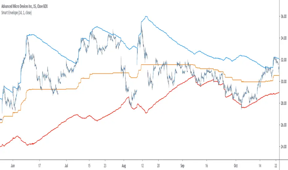
Smart Envelope - Running Away From The TrendIntroduction
Envelopes indicators consist in displaying one upper and one lower extremity on the price chart. They are most of the time built by adding/subtracting a volatility estimator (rolling stdev, atr, range...etc) to a central tendency estimator (SMA, EMA, LSMA...etc) . Their interpretation is often subject to debate amongst technical analyst, some will use a support and resistance methodology, where price will start a downtrend once it cross the upper extremity, and a down trend once it cross the lower one. Others will prefer a breakout methodology, where price will reach higher highs once it cross the upper extremity, and lower lows when it cross the lower one. Because of price non stationarity its hard to select the best methodology, the support and resistance one will mostly work on ranging markets, while the breakout methodology mostly work on trending ones.
Therefore new methods where proposed, instead of using moving averages with a high lag, faster filters where used, such as the least squares moving average or zero lag exponential moving average, other band indicators where also created using adaptive filters, but improvements remain relatively low. The most difficult task would be to make extremities with the ability to return accurate support and resistances levels, and today i want to provide a new way to construct such extremities by using the recursive bands framework that allow extremely creative and efficient indicators.
The Main Idea
With classical bands indicators, the upper and lower extremity will still be correlated with the main trend, the problem behind such method is that we can't use a support and resistance methodology with trending markets, the fact that reversals exist tells us that our extremities will always be crossed by the main trend, here is an example :
Here the support is correlated with the main trend, in order for it to be accurate we must assume the trend will go on for ever, and will only detect higher lows, this is what we expect with the orange line, but we can see that a severe down trend totally destroy our plan.
In short we need to give some headroom to our extremities, and thus one extremity can't be correlated with the main trend.
The proposed Indicator
We want to minimize the correlation between the extremities, so if the upper extremity rise, the lower one must fall. This allow to give some headroom and allow the user to anticipate larger movements, this is how bands seeking to give support and resistances points should work.
The indicator has a length setting that control the wideness of the extremities, unlike other indicators low values such as 14 can still create really wide bands, take that into account.
length = 5. Lower length values allow for more motion from the extremities, but does not necessarily involve detecting shorter terms support and resistances levels. The factor setting is not that important, but it allow to return extremities with more motion when high, and really wide bands when below 1 and greater than 0.
Central Tendency Estimator
Something fun with the recursive band framework is that the bands are no longer based on the central tendency estimator but its the central tendency estimator who is based on the bands. The central tendency estimator can also provide support and resistances points with the price, like classical moving averages, altho its lack of motion is this time a downside.
Conclusion
Altho the extremities are more accurate than other band indicators, the problem remain the same, larger trend will always break the extremities and continue creating higher/lower highs/lows, at this point our stop loss would certainly be triggered. This is a huge downsides of contrarian strategy, we sure might anticipate reversals earlier, but we are exposed to larger price movements, therefore the risk is extreme.
But the proposed methodology might still prove useful to develop more robust support and resistances levels based on envelopes indicators.
Thanks for reading !
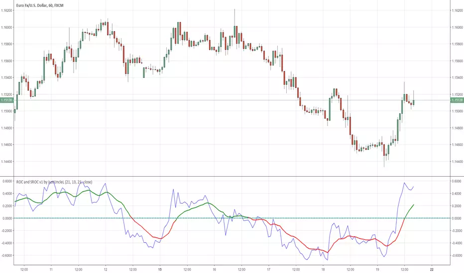
ROC and SROC v1 by JustUncleLDescription:
This study plots a combination Rate of Change Indicator (ROC) and Smoothed Rate of Change (SROC) indicators.
The ROC and SROC are momentum indicators and can be used in ranging or trending markets, please refer to the references for further details of how to use the indicators.
References:
www.incrediblecharts.com
www.incrediblecharts.com
BUY & SELL PRESSURE XeLMod V2BUY & SELL PRESSURE Oscillator
Ver. 2.0 XelMod
WHAT'S THIS?
This is an UPDATED version of a previous script already posted.
List of changes from previous script:
Separated as Column Histogram just the Regressive (Rate-Of-Change) Force of the indicator which gives a faster response of the trend.
Default period is now set to 81, as better Oscillator swing lagging.
This is an excelent momentum indicator very similar to ADX but in a candle weighting distribution rather than ranges.
For additional reference:
Karthik Marar BUY AND SELL PRESSURE INDICATORS.
Cheers!
Any feedback will be welcome...
@XeL_Arjona

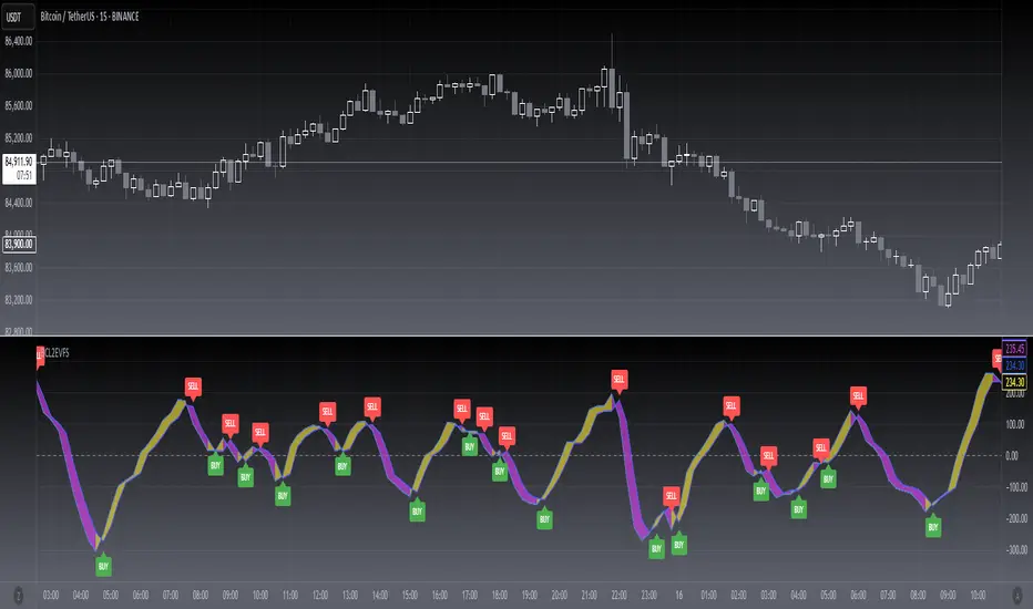
AekFreedom Trading OscillatorAekFreedom Trading Oscillator: User Guide
Overview
The AekFreedom Trading Oscillator is a comprehensive, all-in-one technical analysis tool designed for TradingView. It consolidates a powerful suite of essential indicators into a single, highly customizable indicator pane. The primary goal is to reduce chart clutter and provide traders with a multi-faceted view of the market, combining momentum, trend strength, volatility, and divergence signals in one place.
Core Features & Indicators
This script includes the following fully customizable indicators:
Relative Strength Index (RSI): A core momentum oscillator used to measure the speed and change of price movements. It features gradient fills for overbought (70-100) and oversold (0-30) zones, along with an optional smoothing moving average.
Stochastic Oscillator: Another momentum indicator that compares a particular closing price of a security to a range of its prices over a certain period of time to identify overbought and oversold conditions.
MACD (Moving Average Convergence Divergence): A trend-following momentum indicator that shows the relationship between two exponential moving averages (EMAs). It includes the MACD line, Signal line, and Histogram.
Awesome Oscillator (AO): A momentum indicator that measures the market's driving force by comparing recent momentum with general momentum over a wider timeframe.
ADX (Average Directional Index): An indicator used to quantify the strength of a trend, regardless of its direction (up or down). An ADX value over 25 typically suggests a strong trend.
ATR (Average True Range): A key indicator for measuring market volatility.
Advanced Divergence Engine
One of the most powerful features of this script is its built-in Divergence Engine. It can automatically detect and display both Regular Bullish and Regular Bearish divergences.
Supported Indicators: Divergence detection is available for RSI, Awesome Oscillator (AO), and the MACD Line.
Visual Signals: When a divergence is found, the script will:
Draw a line on the oscillator connecting the relevant pivot points.
Display a "Bull" or "Bear" label directly below or above the signal for easy identification.
Alerts: You can set up alerts in TradingView that will trigger whenever a new divergence signal appears.
How to Use: Settings Panel
The indicator is fully customizable via the settings panel.
Indicator Visibility
This is your main control panel for toggling visuals on and off to keep your chart clean.
Show...: Check or uncheck any indicator (e.g., Show RSI & MA, Show Stochastic, Show ATR) to display or hide it instantly.
Show... Divergence: Use these checkboxes (e.g., Show RSI Divergence) to control the visibility of the divergence lines and labels on the chart.
Indicator-Specific Settings
Each indicator has its own group of settings for fine-tuning its parameters.
RSI / AO / MACD Settings:
Here you can adjust standard parameters like Length, Source, etc.
IMPORTANT: Each of these has a Calculate Divergence checkbox. You must enable this checkbox for the script to perform the resource-intensive calculation for that indicator's divergence.
Stochastic Settings: Adjust the %K Length, %K Smoothing, and %D Smoothing.
ADX Settings: Adjust the ADX Smoothing and DI Length.
ATR Settings: Adjust the Length for the ATR calculation.
📌 How to Enable Divergence Signals (2 Steps):
To see divergence for an indicator (e.g., MACD), you must do two things:
Go to "MACD Settings" and check the box for Calculate Divergence.
Go to "Indicator Visibility" and ensure the box for Show MACD Divergence is also checked.

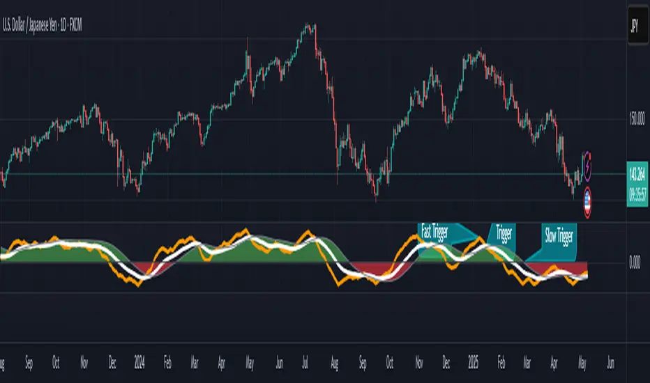
Parsifal.Swing.TrendScoreThe Parsifal.Swing.TrendScore indicator is a module within the Parsifal Swing Suite, which includes a set of swing indicators such as:
• Parsifal Swing TrendScore
• Parsifal Swing Composite
• Parsifal Swing RSI
• Parsifal Swing Flow
Each module serves as an indicator facilitating judgment of the current swing state in the underlying market.
________________________________________
Background
Market movements typically follow a time-varying trend channel within which prices oscillate. These oscillations—or swings—within the trend are inherently tradable.
They can be approached:
• One-sidedly, aligning with the trend (generally safer), or
• Two-sidedly, aiming to profit from mean reversions as well.
Note: Mean reversions in strong trends often manifest as sideways consolidations, making one-sided trades more stable.
________________________________________
The Parsifal Swing Suite
The modules aim to provide additional insights into the swing state within a trend and offer various trigger points to assist with entry decisions.
All modules in the suite act as weak oscillators, meaning they fluctuate within a range but are not bounded like true oscillators (e.g., RSI, which is constrained between 0% and 100%).
________________________________________
The Parsifal.Swing.TrendScore – Specifics
The Parsifal.Swing.TrendScore module combines short-term trend data with information about the current swing state, derived from raw price data and classical technical indicators. It provides an indication of how well the short-term trend aligns with the prevailing swing, based on recent market behavior.
________________________________________
How Swing.TrendScore Works
The Swing.TrendScore calculates a swing score by collecting data within a bin (i.e., a single candle or time bucket) that signals an upside or downside swing. These signals are then aggregated together with insights from classical swing indicators.
Additionally, it calculates a short-term trend score using core technical signals, including:
• The Z-score of the price's distance from various EMAs
• The slope of EMAs
• Other trend-strength signals from additional technical indicators
These two components—the swing score and the trend score—are then combined to form the Swing.TrendScore indicator, which evaluates the short-term trend in context with swing behavior.
________________________________________
How to Interpret Swing.TrendScore
The trend component enhances Swing.TrendScore’s ability to provide stronger signals when the short-term trend and swing state align.
It can also override the swing score; for example, even if a mean reversion appears to be forming, a dominant short-term trend may still control the market behavior.
This makes Swing.TrendScore particularly valuable for:
• Short-term trend-following strategies
• Medium-term swing trading
Unlike typical swing indicators, Swing.TrendScore is designed to respond more to medium-term swings rather than short-lived fluctuations.
________________________________________
Behavior and Chart Representation
The Swing.TrendScore indicator fluctuates within a range, as most of its components are range-bound (though Z-score components may technically extend beyond).
• Historically high or low values may suggest overbought or oversold conditions
• The chart displays:
o A fast curve (orange)
o A slow curve (white)
o A shaded background representing the market state
• Extreme values followed by curve reversals may signal a developing mean reversion
________________________________________
TrendScore Background Value
The Background Value reflects the combined state of the short-term trend and swing:
• > 0 (shaded green) → Bullish mode: swing and short-term trend both upward
• < 0 (shaded red) → Bearish mode: swing and short-term trend both downward
• The absolute value represents the confidence level in the market mode
Notably, the Background Value can remain positive during short downswings if the short-term trend remains bullish—and vice versa.
________________________________________
How to Use the Parsifal.Swing.TrendScore
Several change points can act as entry triggers or aids:
• Fast Trigger: change in slope of the fast signal curve
• Trigger: fast line crosses slow line or the slope of the slow signal changes
• Slow Trigger: change in sign of the Background Value
Examples of these trigger points are illustrated in the accompanying chart.
Additionally, market highs and lows aligning with the swing indicator values may serve as pivot points in the evolving price process.
________________________________________
As always, this indicator should be used in conjunction with other tools and market context in live trading.
While it provides valuable insight and potential entry points, it does not predict future price action.
Instead, it reflects recent tendencies and should be used judiciously.
________________________________________
Extensions
The aggregation of information—whether derived from bins or technical indicators—is currently performed via simple averaging. However, this can be modified using alternative weighting schemes, based on:
• Historical performance
• Relevance of the data
• Specific market conditions
Smoothing periods used in calculations are also modifiable. In general, the EMAs applied for smoothing can be extended to reflect expectations based on relevance-weighted probability measures.
Since EMAs inherently give more weight to recent data, this allows for adaptive smoothing.
Additionally, EMAs may be further extended to incorporate negative weights, akin to wavelet transform techniques.
Supertrend + MACD Trend Change with AlertsDetailed Guide
1. Indicator Overview
Purpose:
This script combines the Supertrend and MACD indicators to help you detect potential trend changes. It plots a Supertrend line (green for bullish, red for bearish) and marks the chart with shapes when a trend reversal is signaled by both indicators. In addition, it includes alert conditions so that you can be notified when a potential trend change occurs.
How It Works:
Supertrend: Uses the Average True Range (ATR) to determine dynamic support and resistance levels. When the price crosses these levels, it signals a possible change in trend.
MACD: Focuses on the crossover between the MACD line and the signal line. A bullish crossover (MACD line crossing above the signal line) suggests upward momentum, while a bearish crossover (MACD line crossing below the signal line) suggests downward momentum.
2. Supertrend Component
Key Parameters:
Factor:
Function: Multiplies the ATR to create an offset from the mid-price (hl2).
Adjustment Impact: Lower values make the indicator more sensitive (producing more frequent signals), while higher values result in fewer, more confirmed signals.
ATR Period:
Function: Sets the number of bars over which the ATR is calculated.
Adjustment Impact: A shorter period makes the ATR react more quickly to recent price changes (but can be noisy), whereas a longer period provides a smoother volatility measurement.
Trend Calculation:
The script compares the previous close with the dynamically calculated upper and lower bands. If the previous close is above the upper band, the trend is set to bullish (1); if it’s below the lower band, the trend is bearish (-1). The Supertrend line is then plotted in green for bullish trends and red for bearish trends.
3. MACD Component
Key Parameters:
Fast MA (Fast Moving Average):
Function: Represents a shorter-term average, making the MACD line more sensitive to recent price movements.
Slow MA (Slow Moving Average):
Function: Represents a longer-term average to smooth out the MACD line.
Signal Smoothing:
Function: Defines the period for the signal line, which is a smoothed version of the MACD line.
Crossover Logic:
The script uses the crossover() function to detect when the MACD line crosses above the signal line (bullish crossover) and crossunder() to detect when it crosses below (bearish crossover).
4. Combined Signal Logic
How Signals Are Combined:
Bullish Scenario:
When the MACD shows a bullish crossover (MACD line crosses above the signal line) and the Supertrend indicates a bullish trend (green line), a green upward triangle is plotted below the bar.
Bearish Scenario:
When the MACD shows a bearish crossover (MACD line crosses below the signal line) and the Supertrend indicates a bearish trend (red line), a red downward triangle is plotted above the bar.
Rationale:
By combining the signals from both indicators, you increase the likelihood that the detected trend change is reliable, filtering out some false signals.
5. Alert Functionality
Alert Setup in the Code:
The alertcondition() function is used to define conditions under which TradingView can trigger alerts.
There are two alert conditions:
Bullish Alert: Activated when there is a bullish MACD crossover and the Supertrend confirms an uptrend.
Bearish Alert: Activated when there is a bearish MACD crossover and the Supertrend confirms a downtrend.
What Happens When an Alert Triggers:
When one of these conditions is met, TradingView registers the alert condition. You can then create an alert in TradingView (using the alert dialog) and choose one of these alert conditions. Once set up, you’ll receive notifications (via pop-ups, email, or SMS, depending on your settings) whenever a trend change is signaled.
6. User Adjustments and Their Effects
Factor (Supertrend):
Adjustment: Lowering the factor increases sensitivity, resulting in more frequent signals; raising it will filter out some signals, making them potentially more reliable.
ATR Period (Supertrend):
Adjustment: A shorter ATR period makes the indicator more responsive to recent price movements (but can introduce noise), while a longer period smooths out the response.
MACD Parameters (Fast MA, Slow MA, and Signal Smoothing):
Adjustment:
Shortening the Fast MA increases sensitivity, generating earlier signals that might be less reliable.
Lengthening the Slow MA produces a smoother MACD line, reducing noise.
Adjusting the Signal Smoothing changes how quickly the signal line responds to changes in the MACD line.
7. Best Practices and Considerations
Multiple Confirmation:
Even if both indicators signal a trend change, consider confirming with additional analysis such as volume, price action, or other indicators.
Market Conditions:
These indicators tend to perform best in trending markets. In sideways or choppy conditions, you may experience more false alerts.
Backtesting:
Before applying the indicator in live trading, backtest your settings to ensure they suit your trading style and the market conditions.
Risk Management:
Always use proper risk management, including stop-loss orders and appropriate position sizing, as alerts may occasionally produce late or false signals.
Happy trading!

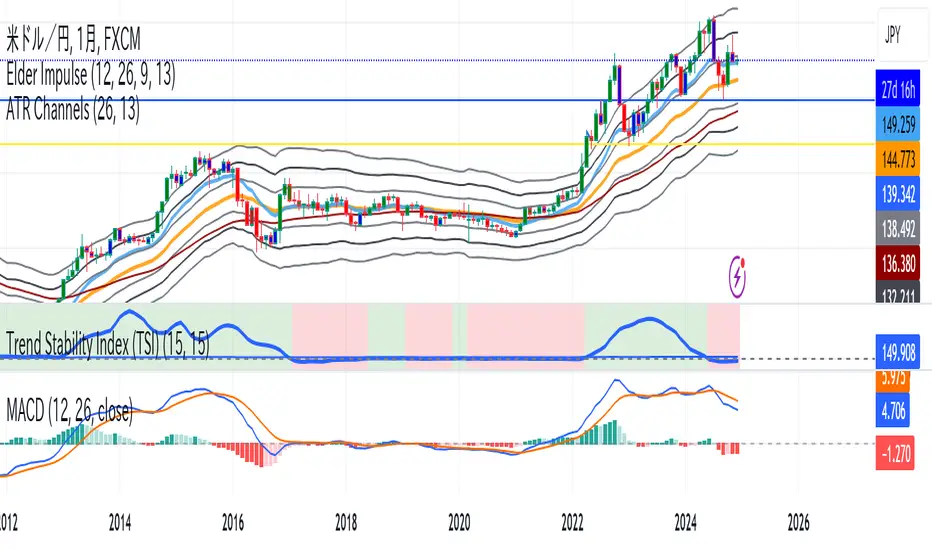
Trend Stability Index (TSI)Overview
The Trend Stability Index (TSI) is a technical analysis tool designed to evaluate the stability of a market trend by analyzing both price movements and trading volume. By combining these two crucial elements, the TSI provides traders with insights into the strength and reliability of ongoing trends, assisting in making informed trading decisions.
Key Features
• Dual Analysis: Integrates price changes and volume fluctuations to assess trend stability.
• Customizable Periods: Allows users to set evaluation periods for both trend and volume based on their trading preferences.
• Visual Indicators: Displays the Trend Stability Index as a line chart, highlights neutral zones, and uses background colors to indicate trend stability or instability.
Configuration Settings
1. Trend Length (trendLength)
• Description: Determines the number of periods over which the price stability is evaluated.
• Default Value: 15
• Usage: A longer trend length smooths out short-term volatility, providing a clearer picture of the overarching trend.
2. Volume Length (volumeLength)
• Description: Sets the number of periods over which trading volume changes are assessed.
• Default Value: 15
• Usage: Adjusting the volume length helps in capturing significant volume movements that may influence trend strength.
Calculation Methodology
The Trend Stability Index is calculated through a series of steps that analyze both price and volume changes:
1. Price Change Rate (priceChange)
• Calculation: Utilizes the Rate of Change (ROC) function on the closing prices over the specified trendLength.
• Purpose: Measures the percentage change in price over the trend evaluation period, indicating the direction and momentum of the price movement.
2. Volume Change Rate (volumeChange)
• Calculation: Applies the Rate of Change (ROC) function to the trading volume over the specified volumeLength.
• Purpose: Assesses the percentage change in trading volume, providing insight into the conviction behind price movements.
3. Trend Stability (trendStability)
• Calculation: Multiplies priceChange by volumeChange.
• Purpose: Combines price and volume changes to gauge the overall stability of the trend. A higher positive value suggests a strong and stable trend, while negative values may indicate trend weakness or reversal.
4. Trend Stability Index (TSI)
• Calculation: Applies a Simple Moving Average (SMA) to the trendStability over the trendLength period.
• Purpose: Smooths the trend stability data to create a more consistent and interpretable index.
Trend/Ranging Determination
• Stable Trend (isStable)
• Condition: When the TSI value is greater than 0.
• Interpretation: Indicates that the current trend is stable and likely to continue in its direction.
• Unstable Trend / Range-bound Market
• Condition: When the TSI value is less than or equal to 0.
• Interpretation: Suggests that the trend may be weakening, reversing, or that the market is moving sideways without a clear direction.
Visualization
The TSI indicator employs several visual elements to convey information effectively:
1. TSI Line
• Representation: Plotted as a blue line.
• Purpose: Displays the Trend Stability Index values over time, allowing traders to observe trend stability dynamics.
2. Neutral Horizontal Line
• Representation: A gray horizontal line at the 0 level.
• Purpose: Serves as a reference point to distinguish between stable and unstable trends.
3. Background Color
• Stable Trend: Green background with 80% transparency when isStable is true.
• Unstable Trend: Red background with 80% transparency when isStable is false.
• Purpose: Provides an immediate visual cue about the current trend’s stability, enhancing the interpretability of the indicator.
Usage Guidelines
• Identifying Trend Strength: Utilize the TSI to confirm the strength of existing trends. A consistently positive TSI suggests strong trend momentum, while a negative TSI may signal caution or a potential reversal.
• Volume Confirmation: The integration of volume changes helps in validating price movements. Significant price changes accompanied by corresponding volume shifts can reinforce the reliability of the trend.
• Entry and Exit Signals: Traders can use crossovers of the TSI with the neutral line (0 level) as potential entry or exit points. For instance, a crossover from below to above 0 may indicate a bullish trend initiation, while a crossover from above to below 0 could suggest bearish momentum.
• Combining with Other Indicators: To enhance trading strategies, consider using the TSI in conjunction with other technical indicators such as Moving Averages, RSI, or MACD for comprehensive market analysis.
Example Scenario
Imagine analyzing a stock with the following observations using the TSI:
• The TSI has been consistently above 0 for the past 30 periods, accompanied by increasing trading volume. This scenario indicates a strong and stable uptrend, suggesting that buying opportunities may be favorable.
• Conversely, if the TSI drops below 0 while the price remains relatively flat and volume decreases, it may imply that the current trend is losing momentum, and the market could be entering a consolidation phase or preparing for a trend reversal.
Conclusion
The Trend Stability Index is a valuable tool for traders seeking to assess the reliability and strength of market trends by integrating price and volume dynamics. Its customizable settings and clear visual indicators make it adaptable to various trading styles and market conditions. By incorporating the TSI into your trading analysis, you can enhance your ability to identify and act upon stable and profitable trends.
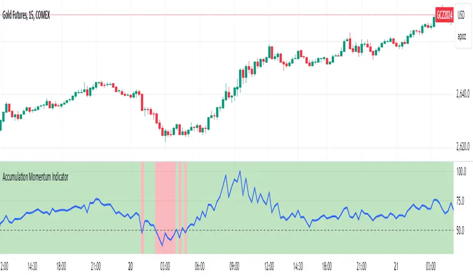
Accumulation Momentum IndicatorEveryone wants to be in a trend, I think this indicator does a great job at showing that key momentum that traders try and capitalize on everyday. I used a Stochastic Momentum Indicator (SMI) indicator. It's a lot like a slower MACD which allows me to capitalize on changing momentum. My goal was to make an indicator that was able to use a weighted mean of many accumulation/momentum indicators. This would give me a well rounded look to really see what direction the momentum and volume is heading.
I did some research on some of the best Accumulation and Momentum Indicators. I landed on 4.
The Accumulation Distribution line which measures the cumulative flow of money in or out of a security. It helps show how quickly money is going in and out of a commodity. The line moving up quickly indicates fast Accumulation while the A/C line is moving down quickly is shows falling Distribution. This can show the momentum and accumulation of a commodity in short and long term based off of Volume.
The On Balance Volume, OBV is a combination of Price Movement and Volume. If price closes higher then the previous bar volume is added while if the price closes lower volume is subtracted. This gives us an overall tally of whether volume is increasing with price or slowing down the momentum in the direction of the current trend. This gives us the ability to see if volume is supporting the price increasing (beginning/middle of a trend) or price is slowing down even though it is still heading in the direction of the current trend (signaling the end of the current trend).
The Force Index, this indicator measures the overall strength of the price movements. It does this by a calculation of price and volume. The close of the current bar subtracted by the previous multiplied by the volume. The result gives us either strong upward or downward motion. This adds magnitude to the overall movement/momentum of the indicator.
Lastly but most certainly not least is the Momentum indicator, (Price Momentum) a simple indicator that shows you the difference between the current close price and the close price from a specified period ago (Most commonly 14 periods/bars ago). Having this indicator is a must because it shows the speed at which price is accelerating or decelerating.
These 4 indicators together help round out the current volume, price movements, accumulation, and momentum of the current market. Since these indicators all have different scales and calculations I had to Normalize the Values to a 0-100 scale. This gives us 1 line and a much more readable easy to understand indicator. After they were normalized I gave them a weighted average that you can control. So lets say you cared more about the Force Index and the OBV rather then the Momentum and the Accumulation Distribution indicators, you would be able to give them more weight in the overall calculation as well as 0 out those you don't even want involved.
I hope the flexibility and the combination of 4 strong Accumulation Momentum indicators helps you better gauge the direction a commodity might head. The way it's used is when the Accumulation Momentum line is Above 50 buying pressure is stronger then selling pressure. An Accumulation Momentum line Below 50 suggests that distribution is more dominant in the current market. This indicator combines four different methods of analyzing price and volume to give you a single composite momentum score, making it easier to visualize when a commodity is being accumulated or distributed and how quickly this process is happening. It helps you track market sentiment based on both price movement and volume, with a clear, visual representation of buying and selling pressure.
Please let me know what you think and how you think I might be able to improve the script. Enjoy!
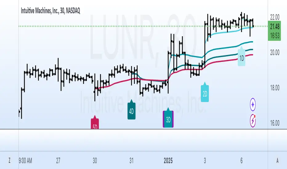
Rolling Strategic AVWAPThe Rolling Strategic AVWAP gives you the ability to have the standard AVWAP indicators applied across all charts in all timeframes. There is no manual intervention necessary to keep all the standard VWAPs up to date. This indicator is written so that all weekends and trading holidays are taken into account so you never have any gaps or days where the indicator isn't working.
Standard rolling AVWAP indicators:
Daily
2-day
3-day
Week-to-Date
Month-to-Date
Year-to-Date
Additionally I have supplied several custom labeled AVWAP indicators that the user can adjust the date themselves
Custom Fixed AVWAP indicators:
Prior Week-to-Date
Prior Month-to-Date
Prior Year-to-Date
Fed rate decision
Inflation report
GDP report
Jobs report
3 more labeled Custom1-3
These custom locations will allow the user to anchor the VWAP to meaningful dates and times in the market. Often there are large moves due to global macro events that can give the trader an edge by referencing the VWAP to the date and time.
Labels and Display
There are options to turn on and off any of the AVWAPs, as well as turning on and off the display labels below the candles.
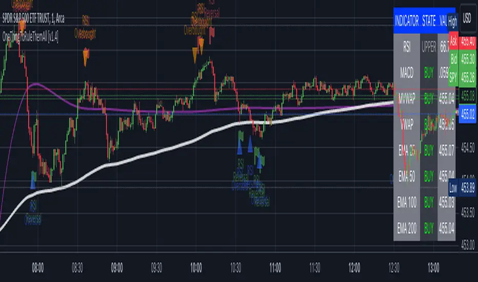
OneThingToRuleThemAll [v1.4]This script was created because I wanted to be able to display a contextual chart of commonly used indicators for scalping and swing traders, with the ability to control the visual representation on the charts as their cross-overs, cross-unders, or changes of state happen in real time. Additionally, I wanted the ability to control how or when they are displayed. While looking through other community projects, I found they lacked the ability to full customize the output controls and values used for these indicators.
The script leverages standard RSI/MACD/VWAP/MVWAP/EMA calculations to help a trader visually make more informed decisions on entering or exiting a trade, depending on their understanding on what the indicators represent. Paired with a table directly on the chart, it allows a trader to quickly reference values to make more informed decisions without having to look away from the price action or look through multiple indicator outputs.
The main functionality of the indicator is controlled within the settings directly on the chart. There a user can enable the visual representations, or disable, and configure how they are displayed on the charts by altering their values or style types.
Users have the ability to enable/disable visual representations of:
The indicator chart
RSI Cross-over and RSI Reversals
MACD Uptrends and Downtrends
VWAP Cross-overs and Cross-unders
VWAP Line
MVWAP Cross-overs and Cross-unders
MVWAP Line
EMA Cross-overs and Cross-unders
EMA Line
Some traders like to use these visual indications as thresholds to enter or exit trades. Its best to find out which ones work the best with the security you are trying to trade. Personally, I use the table as a reference in conjunction with the RSI chart indicators to help me decide a logical trailing stop if I am scalping. Some users might like the track EMA200 crossovers, and have visual representations on the chart for when that happens. However, users may use the other indicators in other methods, and this script provides the ability to be able to configure those both visually and by value.
The pine script code is open source and itself is fairly straightforward, it is mostly written to provide the ultimate level of control the the user of the various indicators. Please reach out to me directly if you would like a further understanding of the code and an explanation on anything that may be unclear.
Enjoy :)
-dead1.
Multi Trend Cross Strategy TemplateToday I am sharing with the community trend cross strategy template that incorporates any combination of over 20 built in indicators. Some of these indicators are in the Pine library, and some have been custom coded and contributed over time by the beloved Pine Coder community. Identifying a trend cross is a common trend following strategy and a common custom-code request from the community. Using this template, users can now select from over 400 different potential trend combinations and setup alerts without any custom coding required. This Multi-Trend cross template has a very inclusive library of trend calculations/indicators built-in, and will plot any of the 20+ indicators/trends that you can select in the settings.
How it works : Simple trend cross strategies go long when the fast trend crosses over the slow trend, and/or go short when the fast trend crosses under the slow trend. Options for either trend direction are built-in to this strategy template. The script is also coded in a way that allows you to enable/modify pyramid settings and scale into a position over time after a trend has crossed.
Use cases : These types of strategies can reduce the volatility of returns and can help avoid large market downswings. For instance, those running a longer term trend-cross strategy may have not realized half the down swing of the bear markets or crashes in 02', 08', 20', etc. However, in other years, they may have exited the market from time to time at unfavorable points that didn't end up being a down turn, or at times the market was ranging sideways. Some also use them to reduce volatility and then add leverage to attempt to beat buy/hold of the underlying asset within an acceptable drawdown threshold.
Special thanks to @Duyck, @everget, @KivancOzbilgic and @LazyBear for coding and contributing earlier versions of some of these custom indicators in Pine.
This script incorporates all of the following indicators. Each of them can be selected and modified from within the indicator settings:
ALMA - Arnaud Legoux Moving Average
DEMA - Double Exponential Moving Average
DSMA - Deviation Scaled Moving Average - Contributed by Everget
EMA - Exponential Moving Average
HMA - Hull Moving Average
JMA - Jurik Moving Average - Contributed by Everget
KAMA - Kaufman's Adaptive Moving Average - Contributed by Everget
LSMA - Linear Regression , Least Squares Moving Average
RMA - Relative Moving Average
SMA - Simple Moving Average
SMMA - Smoothed Moving Average
Price Source - Plotted based on source selection
TEMA - Triple Exponential Moving Average
TMA - Triangular Moving Average
VAMA - Volume Adjusted Moving Average - Contributed by Duyck
VIDYA - Variable Index Dynamic Average - Contributed by KivancOzbilgic
VMA - Variable Moving Average - Contributed by LazyBear
VWMA - Volume Weighted Moving Average
WMA - Weighted Moving Average
WWMA - Welles Wilder's Moving Average
ZLEMA - Zero Lag Exponential Moving Average - Contributed by KivancOzbilgic
Disclaimer : This is not financial advice. Open-source scripts I publish in the community are largely meant to spark ideas that can be used as building blocks for part of a more robust trade management strategy. If you would like to implement a version of any script, I would recommend making significant additions/modifications to the strategy & risk management functions. If you don’t know how to program in Pine, then hire a Pine-coder. We can help!

APA-Adaptive, Ehlers Early Onset Trend [Loxx]APA-Adaptive, Ehlers Early Onset Trend is Ehlers Early Onset Trend but with Autocorrelation Periodogram Algorithm dominant cycle period input.
What is Ehlers Early Onset Trend?
The Onset Trend Detector study is a trend analyzing technical indicator developed by John F. Ehlers , based on a non-linear quotient transform. Two of Mr. Ehlers' previous studies, the Super Smoother Filter and the Roofing Filter, were used and expanded to create this new complex technical indicator. Being a trend-following analysis technique, its main purpose is to address the problem of lag that is common among moving average type indicators.
The Onset Trend Detector first applies the EhlersRoofingFilter to the input data in order to eliminate cyclic components with periods longer than, for example, 100 bars (default value, customizable via input parameters) as those are considered spectral dilation. Filtered data is then subjected to re-filtering by the Super Smoother Filter so that the noise (cyclic components with low length) is reduced to minimum. The period of 10 bars is a default maximum value for a wave cycle to be considered noise; it can be customized via input parameters as well. Once the data is cleared of both noise and spectral dilation, the filter processes it with the automatic gain control algorithm which is widely used in digital signal processing. This algorithm registers the most recent peak value and normalizes it; the normalized value slowly decays until the next peak swing. The ratio of previously filtered value to the corresponding peak value is then quotiently transformed to provide the resulting oscillator. The quotient transform is controlled by the K coefficient: its allowed values are in the range from -1 to +1. K values close to 1 leave the ratio almost untouched, those close to -1 will translate it to around the additive inverse, and those close to zero will collapse small values of the ratio while keeping the higher values high.
Indicator values around 1 signify uptrend and those around -1, downtrend.
What is an adaptive cycle, and what is Ehlers Autocorrelation Periodogram Algorithm?
From his Ehlers' book Cycle Analytics for Traders Advanced Technical Trading Concepts by John F. Ehlers , 2013, page 135:
"Adaptive filters can have several different meanings. For example, Perry Kaufman’s adaptive moving average ( KAMA ) and Tushar Chande’s variable index dynamic average ( VIDYA ) adapt to changes in volatility . By definition, these filters are reactive to price changes, and therefore they close the barn door after the horse is gone.The adaptive filters discussed in this chapter are the familiar Stochastic , relative strength index ( RSI ), commodity channel index ( CCI ), and band-pass filter.The key parameter in each case is the look-back period used to calculate the indicator. This look-back period is commonly a fixed value. However, since the measured cycle period is changing, it makes sense to adapt these indicators to the measured cycle period. When tradable market cycles are observed, they tend to persist for a short while.Therefore, by tuning the indicators to the measure cycle period they are optimized for current conditions and can even have predictive characteristics.
The dominant cycle period is measured using the Autocorrelation Periodogram Algorithm. That dominant cycle dynamically sets the look-back period for the indicators. I employ my own streamlined computation for the indicators that provide smoother and easier to interpret outputs than traditional methods. Further, the indicator codes have been modified to remove the effects of spectral dilation.This basically creates a whole new set of indicators for your trading arsenal."

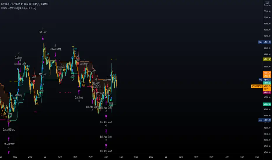
Double SupertrendThis strategy is based on a custom indicator that was created based on the Supertrend indicator. At its core, there are always 2 super trend indicators with different factors to reduce market noise (false signals).
The strategy/indicator has some parameters to improve the signals and filters.
TECHNICAL ANALYSIS
☑ Show Indicators
This option will enable/disable the Supertrend indicators on the chart.
☑ Length
The length will be used on the Supertrend Indicator to calculate its values.
☑ Dev Fast
The fast deviation or factor from one of the super trend indicators. This will be the leading indicator for entry signals, as well as for the exit signals.
☑ Dev Slow
The slow deviation or factor from one of the super trend indicators. This will be the confirmation indicator for entry and exit signals.
☑ Exit Type
It's possible to select from 4 options for the exit signals. Exit signals always take profit target.
☑ ⥹ Reversals
This option will make the strategy/indicator calculate the exit signals based on the difference between the given period's highest and lowest candle value (see Period on this list). It's displayed on the chart with the cross. As it's possible to verify in the image below, there are multiple exit spots for every entry.
☑ ⥹ ATR
Using ATR as a base indicator for exit signals will make the strategy/indicator place limit/stop orders. Candle High + ATR for longs, Candle Low - ATR for shorts. The strategy will show the ATR level for take profit and stick with it until the next signal. This way, the take profit value remains based on the candle of the entry signal.
☑ ⥹ Fast Supertrend
With this option selected, the exit signals will be based on the Fast Supertsignal value, mirrored to make a profit.
☑ ⥹ Slow Supertrend
With this option selected, the exit signals will be based on the Slow Supertsignal value, which is mirrored to take profit.
☑ Period
This will represent the number of candles used on the exit signals when Reversals is selected as Exit Type. It's also used to calculate the gradient used on the Fills and Supertrend signals.
☑ Multiplier
It's used on the take profit when the ATR option is selected on the Exit Type.
STRATEGY
☑ Use The Strategy
This will enable/disable the strategy to show the trades calculations.
☑ Show Use Long/Short Entries
Option to make the strategy show/use Long or Short signals. Available only if Use The Strategy is enabled
☑ Show Use Exit Long/Short
Option to make the strategy show/use Exit Long or Short signals (valid when Reversals option is selected on the Exit Type). Available only if Use The Strategy is enabled
☑ Show Use Add Long/Short
Option to make the strategy show/use Add Long or Short signals. With this option enabled, the strategy will place multiple trades in the same direction, almost the same concept as a pyramiding parameter. It's based on the Fast Supersignal when the candle fails to cross and reverses. Available only if Use The Strategy is enabled
☑ Trades Date Start/End
The date range that the strategy will check the market data and make the trades
HOW TO USE
It's very straightforward. A long signal will appear as a green arrow with a text Long below it. A short signal will appear as a red arrow with a text Short above it. It's ideal to wait for the candle to finish to validate the signal.
The exit signals are optional but give a good idea of the configuration used when backtesting. Each market and timeframe will have its own configuration for the best results. On average, sticking to ATR as an exit signal will have less risk than the other options.
☑ Entry Signals
Follow the arrows with Long/Short texts on them. Wait for the signal candle to close to validate the entry.
☑ Exit Signals
Use them to close your position or to trail stop your orders and maximize profits. Select the exit type suitable for each timeframe and market
☑ Add Entries
It's possible to increase the position following the add margin/contracts based on the Add signals. Not mandatory, but may work as reentries or late entries using the same signal.
☑ What about Stop Loss?
The stop-loss levels were not included as a separated signal because it's already in the chart. There are some possible ideas for the stop loss:
☑⥹ Candle High/Low (2nd recommend option)
When it's a Long signal from the entry signal candle, the stop loss can be the Low value of the same candle. Very tight stop loss in some cases, depending on the candle range
☑⥹ Local Top/Bottom
Selecting the local top/bottom as stop loss will give the strategy more room for false breakouts or reversals, keeping the trade open and minimizing noises. Increases the risk
☑⥹ Fast Supertrend (1st recommend option)
The fast supertrend can be used as stop-loss as well. making it a moving level and working close to trail stop management
☑⥹ Fixed Percentage
It's possible to use a fixed risk percentage for the trades, making the risk easier to control and project. Since the market volatility is not fixed, this may affect the accuracy of the trades
☑⥹ Based on the ATR (3rd recommend option)
When the exit type option ATR is selected, it will display the take profit level for that entry. Just mirror that value and put it as stop-loss, or multiply that amount by 1.5 to have more room for market noise.
EXAMPLE CONFIGURATIONS
Here are some configuration ideas for some markets (all of them are from crypto, especially futures markets)
BTCUSDT 15min - Default configuration
BTCUSDT 1h - Length 10 | Dev Fast 3 | Dev Slow 4 | Exit Type ATR | Period 50 | Multiplier 1
BTCUSDT 4h - Length 10 | Dev Fast 2 | Dev Slow 4 | Exit Type ATR | Period 50 | Multiplier 1
ETHUSDT 15min - Length 20 | Dev Fast 1 | Dev Slow 3 | Exit Type Fast Supertrend | Period 50 | Multiplier 1
IOTAUSDT 15min - Length 10 | Dev Fast 1 | Dev Slow 2 | Exit Type Slow Supertrend | Period 50 | Multiplier 1
OMGUSDT 15min - Length 10 | Dev Fast 1 | Dev Slow 4 | Exit Type Slow Supertrend | Period 50 | Multiplier 1
VETUSDT 15min - Length 10 | Dev Fast 3 | Dev Slow 4 | Exit Type Slow Supertrend | Period 50 | Multiplier 1
HOW TO FIND OTHER CONFIGURATIONS
Here are some steps to find suitable configurations
select a market and time frame
enable the Use This Strategy option on the strategy
open the strategy tester panel and select the performance summary
open the strategy configuration and go to properties
change the balance to the same price of the symbol (example: BTCUSDT 60.000, use 60.000 as balance)
go back to the inputs tab and keep changing the parameters until you see the net profit be positive and bigger than the absolute value of the drawdown
in case you can't find a suitable configuration, try other timeframes
Since the tester reflects what happened in the past candles, it's not guaranteed to give the same results. However, this indicator/Strategy can be used with other indicators as a leading signal or confirmation signal.
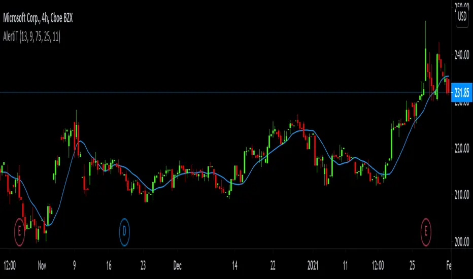
AlertiTI can't be glued to all charts on all tickers all the time. I have a life you know, lol.
So in the spirit of getting fresh air, running errands, working and having fun with family & friends, I setup this AlertiT script.
Three indicators: RSI, SMA and Momentum are used in this script alert.
The alert will be triggered if any of the indicators crosses a specified input.
The message will contain the name of the indicator and its current value.
The default is 13 SMA, 9 RSI +75:-25 and 11 Momentum.
I provided an input in the dialogue box so the variables can be adjusted to suit your needs.
Source is open, high, low, close.
Do your own due diligence, your risk is 100% your responsibility. You win some or you learn some. Consider being charitable with some of your profit to help humankind. Small incremental steps work : If you double a penny a day for a month it = $5,368,709. Good luck and happy trading friends...
*3x lucky 7s of trading*
7pt Trading compass:
Price action, entry/exit
Volume average/direction
Trend, patterns, momentum
Newsworthy current events
Revenue
Earnings
Balance sheet
7 Common mistakes:
+5% portfolio trades, risk management
Beware of analysts motives
Emotions & Opinions
FOMO : bad timing
Lack of planning & discipline
Forgetting restraint
Obdurate repetitive errors, no adaptation
7 Important tools:
Trading View app!, Brokerage UI
Accurate indicators & settings
Wide screen monitor/s
Trading log (pencil & graph paper)
Big organized desk
Reading books, playing chess
Sorted watch-list
Checkout my indicators:
Fibonacci VIP - volume
Fibonacci MA7 - price
pi RSI - trend momentum
TTC - trend channel
AlertiT - notification
www.tradingview.com
[blackcat] L2 Ehlers Voss Filter StrategyLevel: 2
Background
John F. Ehlers introuced Voss Filter Strategy in Aug, 2019.
Function
John Ehlers’ mining of the digital signal processing literature space in his article in this issue, “A Peek Into The Future,” brings us another interesting tool for seeing a bit below the noise surrounding price series to better locate turning points. In “A Peek Into The Future” in Aug, 2019, John Ehlers describes the calculation of a new filter that could help signal cyclical turning points in markets. As described by Dr. Ehlers, the filter has a negative group delay and while an indicator based on it cannot actually see into the future, it may provide the trader with signals in advance of other indicators. Noticing that the indicator accurately tracks the market’s peaks and valleys, Ehlers suggests that simple crossovers of the forward-looking Voss predictor with the two-pole band-pass filter may become the basis of a trading system. Having looked at the paper by Henning Voss, I personally appreciate Ehlers’ ability to reduce the calculus of the Voss presentation to six simple lines of code. I thought that the predictive nature of the VossPredictor would be a good candidate to use for one of the current favorite areas of exploration, self-tuning indicators.
Key Signal
Voss --> Ehlers Voss Filter fast line
Trigger --> Ehlers Voss Filter slow line
Pros and Cons
100% John F. Ehlers definition translation, even variable names are the same. This help readers who would like to use pine to read his book.
Remarks
The 93th script for Blackcat1402 John F. Ehlers Week publication.
Readme
In real life, I am a prolific inventor. I have successfully applied for more than 60 international and regional patents in the past 12 years. But in the past two years or so, I have tried to transfer my creativity to the development of trading strategies. Tradingview is the ideal platform for me. I am selecting and contributing some of the hundreds of scripts to publish in Tradingview community. Welcome everyone to interact with me to discuss these interesting pine scripts.
The scripts posted are categorized into 5 levels according to my efforts or manhours put into these works.
Level 1 : interesting script snippets or distinctive improvement from classic indicators or strategy. Level 1 scripts can usually appear in more complex indicators as a function module or element.
Level 2 : composite indicator/strategy. By selecting or combining several independent or dependent functions or sub indicators in proper way, the composite script exhibits a resonance phenomenon which can filter out noise or fake trading signal to enhance trading confidence level.
Level 3 : comprehensive indicator/strategy. They are simple trading systems based on my strategies. They are commonly containing several or all of entry signal, close signal, stop loss, take profit, re-entry, risk management, and position sizing techniques. Even some interesting fundamental and mass psychological aspects are incorporated.
Level 4 : script snippets or functions that do not disclose source code. Interesting element that can reveal market laws and work as raw material for indicators and strategies. If you find Level 1~2 scripts are helpful, Level 4 is a private version that took me far more efforts to develop.
Level 5 : indicator/strategy that do not disclose source code. private version of Level 3 script with my accumulated script processing skills or a large number of custom functions. I had a private function library built in past two years. Level 5 scripts use many of them to achieve private trading strategy.
[blackcat] L2 Ehlers Dominant Cycle Tuned Bandpass FilterLevel: 2
Background
John F. Ehlers introuced his Dominant Cycle Tuned Bandpass Filter Strategy in Mar, 2008.
Function
In "Measuring Cycle Periods", author John Ehlers presents a very interesting technique of measuring dominant market cycle periods by means of multiple bandpass filtering. By utilizing an approach similar to audio equalizers, the signal (here, the price series) is fed into a set of simple second-order infinite impulse response bandpass filters. Filters are tuned to 8,9,10,...,50 periods. The filter with the highest output represents the dominant cycle. A full-featured formula that implements a high-pass filter and a six-tap low-pass Fir filter on input, then 42 parallel Iir band-pass filters.
I've coded John Ehlers' filter bank to measure the dominant cycle (DC) and the sine and cosine filter components in pine v4 for TradingView, based on John Ehlers' article in this issue, "Measuring Cycle Periods." The CycleFilterDC function plots and returns the DC series and its components, so it's a trivial matter to make use of them in a trading strategy.
Based on John Ehlers' article, "Measuring Cycle Periods," he chose to implement the dominant cycle-tuned bandpass filter response to test Ehlers' suggestion to use the sine and cosine crossovers as buy and sell signals. If the sine closely follows the price pattern as suggested, and the cosine is an effective leading function of the sine, then it seems to make sense that a crossover implementation would work well (Personally, what I observed this is not so accurated as his claims).
What he discovered in his tests was that crossovers happened at frequent intervals, even when price has not moved significantly. This leads to a higher percentage of losing trades, particularly when spread, slippage, and commissions are accounted for. Nevertheless, the cosine crossover was quite effective at identifying reversals very early in many cases, so this indicator could prove quite effective when used alongside other indicators. In particular, the use of an indicator to confirm a certain level of recent volatility, as well as an indicator to confirm significant rate of change, could prove quite helpful.
Key Signal
CosineLine--> Ehlers Dominant Cycle Tuned Bandpass Filter Strategy fast line
SineLine--> Ehlers Dominant Cycle Tuned Bandpass Filter Strategy slow line
Pros and Cons
100% John F. Ehlers definition translation, even variable names are the same. This help readers who would like to use pine to read his book.
Remarks
The 72th script for Blackcat1402 John F. Ehlers Week publication.
NOTE: Although Dr. Ehlers think high of Cosine and Sine wave indicator and trading strategy, my study and trading experience indicated it did not work that well as many other oscillator indicators. However, I would like to keep the original code of Dr. Ehlers for anyone who want to make a deep dive into this kind of indicator or strategy with Cosine and Sine wave.
Readme
In real life, I am a prolific inventor. I have successfully applied for more than 60 international and regional patents in the past 12 years. But in the past two years or so, I have tried to transfer my creativity to the development of trading strategies. Tradingview is the ideal platform for me. I am selecting and contributing some of the hundreds of scripts to publish in Tradingview community. Welcome everyone to interact with me to discuss these interesting pine scripts.
The scripts posted are categorized into 5 levels according to my efforts or manhours put into these works.
Level 1 : interesting script snippets or distinctive improvement from classic indicators or strategy. Level 1 scripts can usually appear in more complex indicators as a function module or element.
Level 2 : composite indicator/strategy. By selecting or combining several independent or dependent functions or sub indicators in proper way, the composite script exhibits a resonance phenomenon which can filter out noise or fake trading signal to enhance trading confidence level.
Level 3 : comprehensive indicator/strategy. They are simple trading systems based on my strategies. They are commonly containing several or all of entry signal, close signal, stop loss, take profit, re-entry, risk management, and position sizing techniques. Even some interesting fundamental and mass psychological aspects are incorporated.
Level 4 : script snippets or functions that do not disclose source code. Interesting element that can reveal market laws and work as raw material for indicators and strategies. If you find Level 1~2 scripts are helpful, Level 4 is a private version that took me far more efforts to develop.
Level 5 : indicator/strategy that do not disclose source code. private version of Level 3 script with my accumulated script processing skills or a large number of custom functions. I had a private function library built in past two years. Level 5 scripts use many of them to achieve private trading strategy.
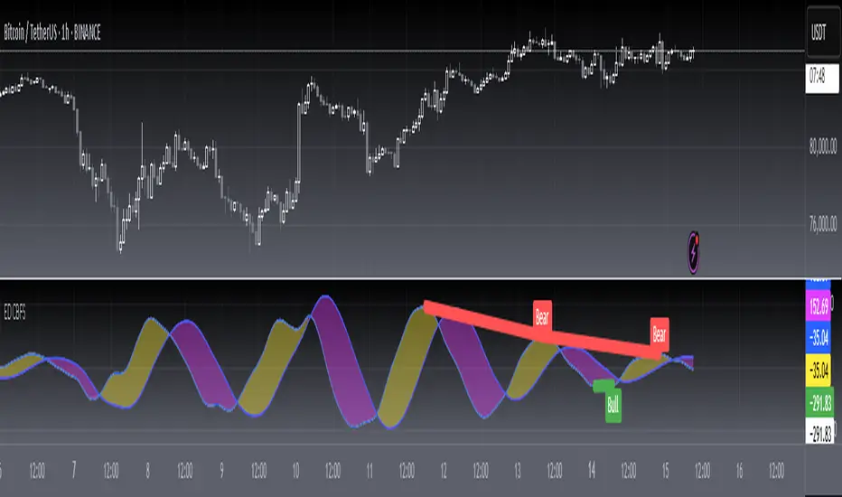
Forward Backward EMA [Repaint]Perform forward-backward filtering using exponential averaging, thus providing a zero-phase exponential moving average. The output repaint and cannot be used as input for other indicators.
Settings
Length : moving average period
Src : data input of the moving average
Plot Color : the color of the displayed plot
Line Width : width of the plotted line
Usages
The main usage of moving averages is to provide an estimate of the underlying trend in the price by removing higher term variations from it. Non-causal (repainting) indicators are limited to offline applications, as such, they are most useful for summary analyses, note that it is still possible to infer from the output of repainting indicators, however since past outputs are subject to changes, it is extremely difficult to track the effectiveness of such indicators, and in online applications they only track the price, making them equally useful for predictive applications than following the direction of an individual candle.
Non-causal filters can be useful in order to have a better view of symbols with a relatively uninformative evolution.
Details
Causal filters have lag, this is the cost of using past observations as inputs, the more past observations you use, the more lag you will obtain (assuming these past observations have non-zero weights). There are various solutions to reduce the lag of a moving average, the most simple one relying on giving higher weights to more recent observations, another one relies on introducing gain in the filter passband, that is amplifying certain variations in the input signal while attenuating/removing higher term ones, finally, we can use adaptive moving averages to avoid excessive lag.
All these previous solutions can be used causally, but they are far from being perfect, as the lag reduction is often done at the cost of smoothness, if we were to keep the original smoothness of the filter while having no lag we would need to use non-causal solutions. The most common solution is to directly use future values as inputs, such moving averages are called "two-sided" moving averages since they use past values as input (left side) as well as future input values (right side), this is equivalent to shifting the results of a moving average backward.
The advantages of two-sided moving averages is that they conserve the original amplitude response of the moving average, however, it won't be possible to compute the most recent values of the moving average (since we won't have access to future values at a certain point), an alternative method heavily used in digital signal processing is forward-backward filtering.
The method consists of applying a filter forward in time, then we apply it once again backward. In order for you to have an easier understanding of this process think about applying a moving average normally starting at time t = 0 , then apply that moving average once again using the previous results as input but start from t = N-1 , that is from the most recent point, and proceed backward, plotting the result from left to right until you get back to t = 0 .
From this, it follows that forward-backward filtering applies a filter twice, the resulting filter is thus a two-passes filter, this results in an even smoother output (more precisely the filter amplitude response is squared).
Forward-backward filtering can be done in Pinescript by using the function "line.new" inside a loop, an exponential moving average is applied forward first, then once again backward inside the loop, "line.new" is used to plot the results backward.
Notes
It is important to note that forward-backward filtering is a repainting process, all the results of the indicator you see on the chart are subject to change over time. Since the method make use of line.new you will have around only 54 visible observations, with the impossibility of using them as input for other indicators. If you see indicators in the future with the same characteristics be aware that they will repaint.
Never purchase/rent filters that appear as having no lag, they are either repainting or the results are coming from a lucky shot or from an overfitted model, it is impossible to make both zero-lag and causal moving averages with pinescript, if you have doubt don't test your luck, better safe than sorry.
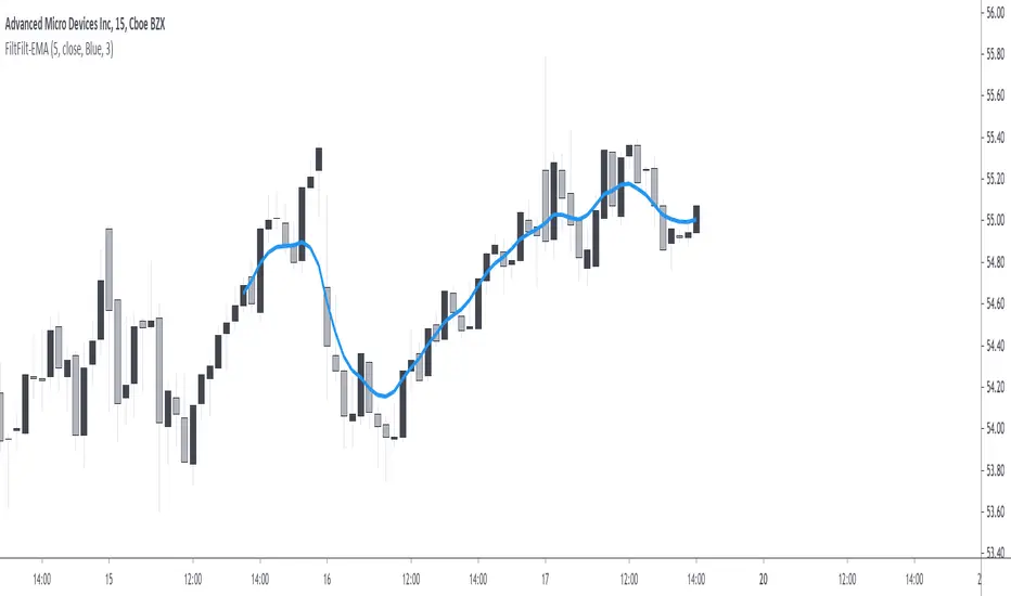
Markov Chain [3D] | FractalystWhat exactly is a Markov Chain?
This indicator uses a Markov Chain model to analyze, quantify, and visualize the transitions between market regimes (Bull, Bear, Neutral) on your chart. It dynamically detects these regimes in real-time, calculates transition probabilities, and displays them as animated 3D spheres and arrows, giving traders intuitive insight into current and future market conditions.
How does a Markov Chain work, and how should I read this spheres-and-arrows diagram?
Think of three weather modes: Sunny, Rainy, Cloudy.
Each sphere is one mode. The loop on a sphere means “stay the same next step” (e.g., Sunny again tomorrow).
The arrows leaving a sphere show where things usually go next if they change (e.g., Sunny moving to Cloudy).
Some paths matter more than others. A more prominent loop means the current mode tends to persist. A more prominent outgoing arrow means a change to that destination is the usual next step.
Direction isn’t symmetric: moving Sunny→Cloudy can behave differently than Cloudy→Sunny.
Now relabel the spheres to markets: Bull, Bear, Neutral.
Spheres: market regimes (uptrend, downtrend, range).
Self‑loop: tendency for the current regime to continue on the next bar.
Arrows: the most common next regime if a switch happens.
How to read: Start at the sphere that matches current bar state. If the loop stands out, expect continuation. If one outgoing path stands out, that switch is the typical next step. Opposite directions can differ (Bear→Neutral doesn’t have to match Neutral→Bear).
What states and transitions are shown?
The three market states visualized are:
Bullish (Bull): Upward or strong-market regime.
Bearish (Bear): Downward or weak-market regime.
Neutral: Sideways or range-bound regime.
Bidirectional animated arrows and probability labels show how likely the market is to move from one regime to another (e.g., Bull → Bear or Neutral → Bull).
How does the regime detection system work?
You can use either built-in price returns (based on adaptive Z-score normalization) or supply three custom indicators (such as volume, oscillators, etc.).
Values are statistically normalized (Z-scored) over a configurable lookback period.
The normalized outputs are classified into Bull, Bear, or Neutral zones.
If using three indicators, their regime signals are averaged and smoothed for robustness.
How are transition probabilities calculated?
On every confirmed bar, the algorithm tracks the sequence of detected market states, then builds a rolling window of transitions.
The code maintains a transition count matrix for all regime pairs (e.g., Bull → Bear).
Transition probabilities are extracted for each possible state change using Laplace smoothing for numerical stability, and frequently updated in real-time.
What is unique about the visualization?
3D animated spheres represent each regime and change visually when active.
Animated, bidirectional arrows reveal transition probabilities and allow you to see both dominant and less likely regime flows.
Particles (moving dots) animate along the arrows, enhancing the perception of regime flow direction and speed.
All elements dynamically update with each new price bar, providing a live market map in an intuitive, engaging format.
Can I use custom indicators for regime classification?
Yes! Enable the "Custom Indicators" switch and select any three chart series as inputs. These will be normalized and combined (each with equal weight), broadening the regime classification beyond just price-based movement.
What does the “Lookback Period” control?
Lookback Period (default: 100) sets how much historical data builds the probability matrix. Shorter periods adapt faster to regime changes but may be noisier. Longer periods are more stable but slower to adapt.
How is this different from a Hidden Markov Model (HMM)?
It sets the window for both regime detection and probability calculations. Lower values make the system more reactive, but potentially noisier. Higher values smooth estimates and make the system more robust.
How is this Markov Chain different from a Hidden Markov Model (HMM)?
Markov Chain (as here): All market regimes (Bull, Bear, Neutral) are directly observable on the chart. The transition matrix is built from actual detected regimes, keeping the model simple and interpretable.
Hidden Markov Model: The actual regimes are unobservable ("hidden") and must be inferred from market output or indicator "emissions" using statistical learning algorithms. HMMs are more complex, can capture more subtle structure, but are harder to visualize and require additional machine learning steps for training.
A standard Markov Chain models transitions between observable states using a simple transition matrix, while a Hidden Markov Model assumes the true states are hidden (latent) and must be inferred from observable “emissions” like price or volume data. In practical terms, a Markov Chain is transparent and easier to implement and interpret; an HMM is more expressive but requires statistical inference to estimate hidden states from data.
Markov Chain: states are observable; you directly count or estimate transition probabilities between visible states. This makes it simpler, faster, and easier to validate and tune.
HMM: states are hidden; you only observe emissions generated by those latent states. Learning involves machine learning/statistical algorithms (commonly Baum–Welch/EM for training and Viterbi for decoding) to infer both the transition dynamics and the most likely hidden state sequence from data.
How does the indicator avoid “repainting” or look-ahead bias?
All regime changes and matrix updates happen only on confirmed (closed) bars, so no future data is leaked, ensuring reliable real-time operation.
Are there practical tuning tips?
Tune the Lookback Period for your asset/timeframe: shorter for fast markets, longer for stability.
Use custom indicators if your asset has unique regime drivers.
Watch for rapid changes in transition probabilities as early warning of a possible regime shift.
Who is this indicator for?
Quants and quantitative researchers exploring probabilistic market modeling, especially those interested in regime-switching dynamics and Markov models.
Programmers and system developers who need a probabilistic regime filter for systematic and algorithmic backtesting:
The Markov Chain indicator is ideally suited for programmatic integration via its bias output (1 = Bull, 0 = Neutral, -1 = Bear).
Although the visualization is engaging, the core output is designed for automated, rules-based workflows—not for discretionary/manual trading decisions.
Developers can connect the indicator’s output directly to their Pine Script logic (using input.source()), allowing rapid and robust backtesting of regime-based strategies.
It acts as a plug-and-play regime filter: simply plug the bias output into your entry/exit logic, and you have a scientifically robust, probabilistically-derived signal for filtering, timing, position sizing, or risk regimes.
The MC's output is intentionally "trinary" (1/0/-1), focusing on clear regime states for unambiguous decision-making in code. If you require nuanced, multi-probability or soft-label state vectors, consider expanding the indicator or stacking it with a probability-weighted logic layer in your scripting.
Because it avoids subjectivity, this approach is optimal for systematic quants, algo developers building backtested, repeatable strategies based on probabilistic regime analysis.
What's the mathematical foundation behind this?
The mathematical foundation behind this Markov Chain indicator—and probabilistic regime detection in finance—draws from two principal models: the (standard) Markov Chain and the Hidden Markov Model (HMM).
How to use this indicator programmatically?
The Markov Chain indicator automatically exports a bias value (+1 for Bullish, -1 for Bearish, 0 for Neutral) as a plot visible in the Data Window. This allows you to integrate its regime signal into your own scripts and strategies for backtesting, automation, or live trading.
Step-by-Step Integration with Pine Script (input.source)
Add the Markov Chain indicator to your chart.
This must be done first, since your custom script will "pull" the bias signal from the indicator's plot.
In your strategy, create an input using input.source()
Example:
//@version=5
strategy("MC Bias Strategy Example")
mcBias = input.source(close, "MC Bias Source")
After saving, go to your script’s settings. For the “MC Bias Source” input, select the plot/output of the Markov Chain indicator (typically its bias plot).
Use the bias in your trading logic
Example (long only on Bull, flat otherwise):
if mcBias == 1
strategy.entry("Long", strategy.long)
else
strategy.close("Long")
For more advanced workflows, combine mcBias with additional filters or trailing stops.
How does this work behind-the-scenes?
TradingView’s input.source() lets you use any plot from another indicator as a real-time, “live” data feed in your own script (source).
The selected bias signal is available to your Pine code as a variable, enabling logical decisions based on regime (trend-following, mean-reversion, etc.).
This enables powerful strategy modularity : decouple regime detection from entry/exit logic, allowing fast experimentation without rewriting core signal code.
Integrating 45+ Indicators with Your Markov Chain — How & Why
The Enhanced Custom Indicators Export script exports a massive suite of over 45 technical indicators—ranging from classic momentum (RSI, MACD, Stochastic, etc.) to trend, volume, volatility, and oscillator tools—all pre-calculated, centered/scaled, and available as plots.
// Enhanced Custom Indicators Export - 45 Technical Indicators
// Comprehensive technical analysis suite for advanced market regime detection
//@version=6
indicator('Enhanced Custom Indicators Export | Fractalyst', shorttitle='Enhanced CI Export', overlay=false, scale=scale.right, max_labels_count=500, max_lines_count=500)
// |----- Input Parameters -----| //
momentum_group = "Momentum Indicators"
trend_group = "Trend Indicators"
volume_group = "Volume Indicators"
volatility_group = "Volatility Indicators"
oscillator_group = "Oscillator Indicators"
display_group = "Display Settings"
// Common lengths
length_14 = input.int(14, "Standard Length (14)", minval=1, maxval=100, group=momentum_group)
length_20 = input.int(20, "Medium Length (20)", minval=1, maxval=200, group=trend_group)
length_50 = input.int(50, "Long Length (50)", minval=1, maxval=200, group=trend_group)
// Display options
show_table = input.bool(true, "Show Values Table", group=display_group)
table_size = input.string("Small", "Table Size", options= , group=display_group)
// |----- MOMENTUM INDICATORS (15 indicators) -----| //
// 1. RSI (Relative Strength Index)
rsi_14 = ta.rsi(close, length_14)
rsi_centered = rsi_14 - 50
// 2. Stochastic Oscillator
stoch_k = ta.stoch(close, high, low, length_14)
stoch_d = ta.sma(stoch_k, 3)
stoch_centered = stoch_k - 50
// 3. Williams %R
williams_r = ta.stoch(close, high, low, length_14) - 100
// 4. MACD (Moving Average Convergence Divergence)
= ta.macd(close, 12, 26, 9)
// 5. Momentum (Rate of Change)
momentum = ta.mom(close, length_14)
momentum_pct = (momentum / close ) * 100
// 6. Rate of Change (ROC)
roc = ta.roc(close, length_14)
// 7. Commodity Channel Index (CCI)
cci = ta.cci(close, length_20)
// 8. Money Flow Index (MFI)
mfi = ta.mfi(close, length_14)
mfi_centered = mfi - 50
// 9. Awesome Oscillator (AO)
ao = ta.sma(hl2, 5) - ta.sma(hl2, 34)
// 10. Accelerator Oscillator (AC)
ac = ao - ta.sma(ao, 5)
// 11. Chande Momentum Oscillator (CMO)
cmo = ta.cmo(close, length_14)
// 12. Detrended Price Oscillator (DPO)
dpo = close - ta.sma(close, length_20)
// 13. Price Oscillator (PPO)
ppo = ta.sma(close, 12) - ta.sma(close, 26)
ppo_pct = (ppo / ta.sma(close, 26)) * 100
// 14. TRIX
trix_ema1 = ta.ema(close, length_14)
trix_ema2 = ta.ema(trix_ema1, length_14)
trix_ema3 = ta.ema(trix_ema2, length_14)
trix = ta.roc(trix_ema3, 1) * 10000
// 15. Klinger Oscillator
klinger = ta.ema(volume * (high + low + close) / 3, 34) - ta.ema(volume * (high + low + close) / 3, 55)
// 16. Fisher Transform
fisher_hl2 = 0.5 * (hl2 - ta.lowest(hl2, 10)) / (ta.highest(hl2, 10) - ta.lowest(hl2, 10)) - 0.25
fisher = 0.5 * math.log((1 + fisher_hl2) / (1 - fisher_hl2))
// 17. Stochastic RSI
stoch_rsi = ta.stoch(rsi_14, rsi_14, rsi_14, length_14)
stoch_rsi_centered = stoch_rsi - 50
// 18. Relative Vigor Index (RVI)
rvi_num = ta.swma(close - open)
rvi_den = ta.swma(high - low)
rvi = rvi_den != 0 ? rvi_num / rvi_den : 0
// 19. Balance of Power (BOP)
bop = (close - open) / (high - low)
// |----- TREND INDICATORS (10 indicators) -----| //
// 20. Simple Moving Average Momentum
sma_20 = ta.sma(close, length_20)
sma_momentum = ((close - sma_20) / sma_20) * 100
// 21. Exponential Moving Average Momentum
ema_20 = ta.ema(close, length_20)
ema_momentum = ((close - ema_20) / ema_20) * 100
// 22. Parabolic SAR
sar = ta.sar(0.02, 0.02, 0.2)
sar_trend = close > sar ? 1 : -1
// 23. Linear Regression Slope
lr_slope = ta.linreg(close, length_20, 0) - ta.linreg(close, length_20, 1)
// 24. Moving Average Convergence (MAC)
mac = ta.sma(close, 10) - ta.sma(close, 30)
// 25. Trend Intensity Index (TII)
tii_sum = 0.0
for i = 1 to length_20
tii_sum += close > close ? 1 : 0
tii = (tii_sum / length_20) * 100
// 26. Ichimoku Cloud Components
ichimoku_tenkan = (ta.highest(high, 9) + ta.lowest(low, 9)) / 2
ichimoku_kijun = (ta.highest(high, 26) + ta.lowest(low, 26)) / 2
ichimoku_signal = ichimoku_tenkan > ichimoku_kijun ? 1 : -1
// 27. MESA Adaptive Moving Average (MAMA)
mama_alpha = 2.0 / (length_20 + 1)
mama = ta.ema(close, length_20)
mama_momentum = ((close - mama) / mama) * 100
// 28. Zero Lag Exponential Moving Average (ZLEMA)
zlema_lag = math.round((length_20 - 1) / 2)
zlema_data = close + (close - close )
zlema = ta.ema(zlema_data, length_20)
zlema_momentum = ((close - zlema) / zlema) * 100
// |----- VOLUME INDICATORS (6 indicators) -----| //
// 29. On-Balance Volume (OBV)
obv = ta.obv
// 30. Volume Rate of Change (VROC)
vroc = ta.roc(volume, length_14)
// 31. Price Volume Trend (PVT)
pvt = ta.pvt
// 32. Negative Volume Index (NVI)
nvi = 0.0
nvi := volume < volume ? nvi + ((close - close ) / close ) * nvi : nvi
// 33. Positive Volume Index (PVI)
pvi = 0.0
pvi := volume > volume ? pvi + ((close - close ) / close ) * pvi : pvi
// 34. Volume Oscillator
vol_osc = ta.sma(volume, 5) - ta.sma(volume, 10)
// 35. Ease of Movement (EOM)
eom_distance = high - low
eom_box_height = volume / 1000000
eom = eom_box_height != 0 ? eom_distance / eom_box_height : 0
eom_sma = ta.sma(eom, length_14)
// 36. Force Index
force_index = volume * (close - close )
force_index_sma = ta.sma(force_index, length_14)
// |----- VOLATILITY INDICATORS (10 indicators) -----| //
// 37. Average True Range (ATR)
atr = ta.atr(length_14)
atr_pct = (atr / close) * 100
// 38. Bollinger Bands Position
bb_basis = ta.sma(close, length_20)
bb_dev = 2.0 * ta.stdev(close, length_20)
bb_upper = bb_basis + bb_dev
bb_lower = bb_basis - bb_dev
bb_position = bb_dev != 0 ? (close - bb_basis) / bb_dev : 0
bb_width = bb_dev != 0 ? (bb_upper - bb_lower) / bb_basis * 100 : 0
// 39. Keltner Channels Position
kc_basis = ta.ema(close, length_20)
kc_range = ta.ema(ta.tr, length_20)
kc_upper = kc_basis + (2.0 * kc_range)
kc_lower = kc_basis - (2.0 * kc_range)
kc_position = kc_range != 0 ? (close - kc_basis) / kc_range : 0
// 40. Donchian Channels Position
dc_upper = ta.highest(high, length_20)
dc_lower = ta.lowest(low, length_20)
dc_basis = (dc_upper + dc_lower) / 2
dc_position = (dc_upper - dc_lower) != 0 ? (close - dc_basis) / (dc_upper - dc_lower) : 0
// 41. Standard Deviation
std_dev = ta.stdev(close, length_20)
std_dev_pct = (std_dev / close) * 100
// 42. Relative Volatility Index (RVI)
rvi_up = ta.stdev(close > close ? close : 0, length_14)
rvi_down = ta.stdev(close < close ? close : 0, length_14)
rvi_total = rvi_up + rvi_down
rvi_volatility = rvi_total != 0 ? (rvi_up / rvi_total) * 100 : 50
// 43. Historical Volatility
hv_returns = math.log(close / close )
hv = ta.stdev(hv_returns, length_20) * math.sqrt(252) * 100
// 44. Garman-Klass Volatility
gk_vol = math.log(high/low) * math.log(high/low) - (2*math.log(2)-1) * math.log(close/open) * math.log(close/open)
gk_volatility = math.sqrt(ta.sma(gk_vol, length_20)) * 100
// 45. Parkinson Volatility
park_vol = math.log(high/low) * math.log(high/low)
parkinson = math.sqrt(ta.sma(park_vol, length_20) / (4 * math.log(2))) * 100
// 46. Rogers-Satchell Volatility
rs_vol = math.log(high/close) * math.log(high/open) + math.log(low/close) * math.log(low/open)
rogers_satchell = math.sqrt(ta.sma(rs_vol, length_20)) * 100
// |----- OSCILLATOR INDICATORS (5 indicators) -----| //
// 47. Elder Ray Index
elder_bull = high - ta.ema(close, 13)
elder_bear = low - ta.ema(close, 13)
elder_power = elder_bull + elder_bear
// 48. Schaff Trend Cycle (STC)
stc_macd = ta.ema(close, 23) - ta.ema(close, 50)
stc_k = ta.stoch(stc_macd, stc_macd, stc_macd, 10)
stc_d = ta.ema(stc_k, 3)
stc = ta.stoch(stc_d, stc_d, stc_d, 10)
// 49. Coppock Curve
coppock_roc1 = ta.roc(close, 14)
coppock_roc2 = ta.roc(close, 11)
coppock = ta.wma(coppock_roc1 + coppock_roc2, 10)
// 50. Know Sure Thing (KST)
kst_roc1 = ta.roc(close, 10)
kst_roc2 = ta.roc(close, 15)
kst_roc3 = ta.roc(close, 20)
kst_roc4 = ta.roc(close, 30)
kst = ta.sma(kst_roc1, 10) + 2*ta.sma(kst_roc2, 10) + 3*ta.sma(kst_roc3, 10) + 4*ta.sma(kst_roc4, 15)
// 51. Percentage Price Oscillator (PPO)
ppo_line = ((ta.ema(close, 12) - ta.ema(close, 26)) / ta.ema(close, 26)) * 100
ppo_signal = ta.ema(ppo_line, 9)
ppo_histogram = ppo_line - ppo_signal
// |----- PLOT MAIN INDICATORS -----| //
// Plot key momentum indicators
plot(rsi_centered, title="01_RSI_Centered", color=color.purple, linewidth=1)
plot(stoch_centered, title="02_Stoch_Centered", color=color.blue, linewidth=1)
plot(williams_r, title="03_Williams_R", color=color.red, linewidth=1)
plot(macd_histogram, title="04_MACD_Histogram", color=color.orange, linewidth=1)
plot(cci, title="05_CCI", color=color.green, linewidth=1)
// Plot trend indicators
plot(sma_momentum, title="06_SMA_Momentum", color=color.navy, linewidth=1)
plot(ema_momentum, title="07_EMA_Momentum", color=color.maroon, linewidth=1)
plot(sar_trend, title="08_SAR_Trend", color=color.teal, linewidth=1)
plot(lr_slope, title="09_LR_Slope", color=color.lime, linewidth=1)
plot(mac, title="10_MAC", color=color.fuchsia, linewidth=1)
// Plot volatility indicators
plot(atr_pct, title="11_ATR_Pct", color=color.yellow, linewidth=1)
plot(bb_position, title="12_BB_Position", color=color.aqua, linewidth=1)
plot(kc_position, title="13_KC_Position", color=color.olive, linewidth=1)
plot(std_dev_pct, title="14_StdDev_Pct", color=color.silver, linewidth=1)
plot(bb_width, title="15_BB_Width", color=color.gray, linewidth=1)
// Plot volume indicators
plot(vroc, title="16_VROC", color=color.blue, linewidth=1)
plot(eom_sma, title="17_EOM", color=color.red, linewidth=1)
plot(vol_osc, title="18_Vol_Osc", color=color.green, linewidth=1)
plot(force_index_sma, title="19_Force_Index", color=color.orange, linewidth=1)
plot(obv, title="20_OBV", color=color.purple, linewidth=1)
// Plot additional oscillators
plot(ao, title="21_Awesome_Osc", color=color.navy, linewidth=1)
plot(cmo, title="22_CMO", color=color.maroon, linewidth=1)
plot(dpo, title="23_DPO", color=color.teal, linewidth=1)
plot(trix, title="24_TRIX", color=color.lime, linewidth=1)
plot(fisher, title="25_Fisher", color=color.fuchsia, linewidth=1)
// Plot more momentum indicators
plot(mfi_centered, title="26_MFI_Centered", color=color.yellow, linewidth=1)
plot(ac, title="27_AC", color=color.aqua, linewidth=1)
plot(ppo_pct, title="28_PPO_Pct", color=color.olive, linewidth=1)
plot(stoch_rsi_centered, title="29_StochRSI_Centered", color=color.silver, linewidth=1)
plot(klinger, title="30_Klinger", color=color.gray, linewidth=1)
// Plot trend continuation
plot(tii, title="31_TII", color=color.blue, linewidth=1)
plot(ichimoku_signal, title="32_Ichimoku_Signal", color=color.red, linewidth=1)
plot(mama_momentum, title="33_MAMA_Momentum", color=color.green, linewidth=1)
plot(zlema_momentum, title="34_ZLEMA_Momentum", color=color.orange, linewidth=1)
plot(bop, title="35_BOP", color=color.purple, linewidth=1)
// Plot volume continuation
plot(nvi, title="36_NVI", color=color.navy, linewidth=1)
plot(pvi, title="37_PVI", color=color.maroon, linewidth=1)
plot(momentum_pct, title="38_Momentum_Pct", color=color.teal, linewidth=1)
plot(roc, title="39_ROC", color=color.lime, linewidth=1)
plot(rvi, title="40_RVI", color=color.fuchsia, linewidth=1)
// Plot volatility continuation
plot(dc_position, title="41_DC_Position", color=color.yellow, linewidth=1)
plot(rvi_volatility, title="42_RVI_Volatility", color=color.aqua, linewidth=1)
plot(hv, title="43_Historical_Vol", color=color.olive, linewidth=1)
plot(gk_volatility, title="44_GK_Volatility", color=color.silver, linewidth=1)
plot(parkinson, title="45_Parkinson_Vol", color=color.gray, linewidth=1)
// Plot final oscillators
plot(rogers_satchell, title="46_RS_Volatility", color=color.blue, linewidth=1)
plot(elder_power, title="47_Elder_Power", color=color.red, linewidth=1)
plot(stc, title="48_STC", color=color.green, linewidth=1)
plot(coppock, title="49_Coppock", color=color.orange, linewidth=1)
plot(kst, title="50_KST", color=color.purple, linewidth=1)
// Plot final indicators
plot(ppo_histogram, title="51_PPO_Histogram", color=color.navy, linewidth=1)
plot(pvt, title="52_PVT", color=color.maroon, linewidth=1)
// |----- Reference Lines -----| //
hline(0, "Zero Line", color=color.gray, linestyle=hline.style_dashed, linewidth=1)
hline(50, "Midline", color=color.gray, linestyle=hline.style_dotted, linewidth=1)
hline(-50, "Lower Midline", color=color.gray, linestyle=hline.style_dotted, linewidth=1)
hline(25, "Upper Threshold", color=color.gray, linestyle=hline.style_dotted, linewidth=1)
hline(-25, "Lower Threshold", color=color.gray, linestyle=hline.style_dotted, linewidth=1)
// |----- Enhanced Information Table -----| //
if show_table and barstate.islast
table_position = position.top_right
table_text_size = table_size == "Tiny" ? size.tiny : table_size == "Small" ? size.small : size.normal
var table info_table = table.new(table_position, 3, 18, bgcolor=color.new(color.white, 85), border_width=1, border_color=color.gray)
// Headers
table.cell(info_table, 0, 0, 'Category', text_color=color.black, text_size=table_text_size, bgcolor=color.new(color.blue, 70))
table.cell(info_table, 1, 0, 'Indicator', text_color=color.black, text_size=table_text_size, bgcolor=color.new(color.blue, 70))
table.cell(info_table, 2, 0, 'Value', text_color=color.black, text_size=table_text_size, bgcolor=color.new(color.blue, 70))
// Key Momentum Indicators
table.cell(info_table, 0, 1, 'MOMENTUM', text_color=color.purple, text_size=table_text_size, bgcolor=color.new(color.purple, 90))
table.cell(info_table, 1, 1, 'RSI Centered', text_color=color.purple, text_size=table_text_size)
table.cell(info_table, 2, 1, str.tostring(rsi_centered, '0.00'), text_color=color.purple, text_size=table_text_size)
table.cell(info_table, 0, 2, '', text_color=color.blue, text_size=table_text_size)
table.cell(info_table, 1, 2, 'Stoch Centered', text_color=color.blue, text_size=table_text_size)
table.cell(info_table, 2, 2, str.tostring(stoch_centered, '0.00'), text_color=color.blue, text_size=table_text_size)
table.cell(info_table, 0, 3, '', text_color=color.red, text_size=table_text_size)
table.cell(info_table, 1, 3, 'Williams %R', text_color=color.red, text_size=table_text_size)
table.cell(info_table, 2, 3, str.tostring(williams_r, '0.00'), text_color=color.red, text_size=table_text_size)
table.cell(info_table, 0, 4, '', text_color=color.orange, text_size=table_text_size)
table.cell(info_table, 1, 4, 'MACD Histogram', text_color=color.orange, text_size=table_text_size)
table.cell(info_table, 2, 4, str.tostring(macd_histogram, '0.000'), text_color=color.orange, text_size=table_text_size)
table.cell(info_table, 0, 5, '', text_color=color.green, text_size=table_text_size)
table.cell(info_table, 1, 5, 'CCI', text_color=color.green, text_size=table_text_size)
table.cell(info_table, 2, 5, str.tostring(cci, '0.00'), text_color=color.green, text_size=table_text_size)
// Key Trend Indicators
table.cell(info_table, 0, 6, 'TREND', text_color=color.navy, text_size=table_text_size, bgcolor=color.new(color.navy, 90))
table.cell(info_table, 1, 6, 'SMA Momentum %', text_color=color.navy, text_size=table_text_size)
table.cell(info_table, 2, 6, str.tostring(sma_momentum, '0.00'), text_color=color.navy, text_size=table_text_size)
table.cell(info_table, 0, 7, '', text_color=color.maroon, text_size=table_text_size)
table.cell(info_table, 1, 7, 'EMA Momentum %', text_color=color.maroon, text_size=table_text_size)
table.cell(info_table, 2, 7, str.tostring(ema_momentum, '0.00'), text_color=color.maroon, text_size=table_text_size)
table.cell(info_table, 0, 8, '', text_color=color.teal, text_size=table_text_size)
table.cell(info_table, 1, 8, 'SAR Trend', text_color=color.teal, text_size=table_text_size)
table.cell(info_table, 2, 8, str.tostring(sar_trend, '0'), text_color=color.teal, text_size=table_text_size)
table.cell(info_table, 0, 9, '', text_color=color.lime, text_size=table_text_size)
table.cell(info_table, 1, 9, 'Linear Regression', text_color=color.lime, text_size=table_text_size)
table.cell(info_table, 2, 9, str.tostring(lr_slope, '0.000'), text_color=color.lime, text_size=table_text_size)
// Key Volatility Indicators
table.cell(info_table, 0, 10, 'VOLATILITY', text_color=color.yellow, text_size=table_text_size, bgcolor=color.new(color.yellow, 90))
table.cell(info_table, 1, 10, 'ATR %', text_color=color.yellow, text_size=table_text_size)
table.cell(info_table, 2, 10, str.tostring(atr_pct, '0.00'), text_color=color.yellow, text_size=table_text_size)
table.cell(info_table, 0, 11, '', text_color=color.aqua, text_size=table_text_size)
table.cell(info_table, 1, 11, 'BB Position', text_color=color.aqua, text_size=table_text_size)
table.cell(info_table, 2, 11, str.tostring(bb_position, '0.00'), text_color=color.aqua, text_size=table_text_size)
table.cell(info_table, 0, 12, '', text_color=color.olive, text_size=table_text_size)
table.cell(info_table, 1, 12, 'KC Position', text_color=color.olive, text_size=table_text_size)
table.cell(info_table, 2, 12, str.tostring(kc_position, '0.00'), text_color=color.olive, text_size=table_text_size)
// Key Volume Indicators
table.cell(info_table, 0, 13, 'VOLUME', text_color=color.blue, text_size=table_text_size, bgcolor=color.new(color.blue, 90))
table.cell(info_table, 1, 13, 'Volume ROC', text_color=color.blue, text_size=table_text_size)
table.cell(info_table, 2, 13, str.tostring(vroc, '0.00'), text_color=color.blue, text_size=table_text_size)
table.cell(info_table, 0, 14, '', text_color=color.red, text_size=table_text_size)
table.cell(info_table, 1, 14, 'EOM', text_color=color.red, text_size=table_text_size)
table.cell(info_table, 2, 14, str.tostring(eom_sma, '0.000'), text_color=color.red, text_size=table_text_size)
// Key Oscillators
table.cell(info_table, 0, 15, 'OSCILLATORS', text_color=color.purple, text_size=table_text_size, bgcolor=color.new(color.purple, 90))
table.cell(info_table, 1, 15, 'Awesome Osc', text_color=color.blue, text_size=table_text_size)
table.cell(info_table, 2, 15, str.tostring(ao, '0.000'), text_color=color.blue, text_size=table_text_size)
table.cell(info_table, 0, 16, '', text_color=color.red, text_size=table_text_size)
table.cell(info_table, 1, 16, 'Fisher Transform', text_color=color.red, text_size=table_text_size)
table.cell(info_table, 2, 16, str.tostring(fisher, '0.000'), text_color=color.red, text_size=table_text_size)
// Summary Statistics
table.cell(info_table, 0, 17, 'SUMMARY', text_color=color.black, text_size=table_text_size, bgcolor=color.new(color.gray, 70))
table.cell(info_table, 1, 17, 'Total Indicators: 52', text_color=color.black, text_size=table_text_size)
regime_color = rsi_centered > 10 ? color.green : rsi_centered < -10 ? color.red : color.gray
regime_text = rsi_centered > 10 ? "BULLISH" : rsi_centered < -10 ? "BEARISH" : "NEUTRAL"
table.cell(info_table, 2, 17, regime_text, text_color=regime_color, text_size=table_text_size)
This makes it the perfect “indicator backbone” for quantitative and systematic traders who want to prototype, combine, and test new regime detection models—especially in combination with the Markov Chain indicator.
How to use this script with the Markov Chain for research and backtesting:
Add the Enhanced Indicator Export to your chart.
Every calculated indicator is available as an individual data stream.
Connect the indicator(s) you want as custom input(s) to the Markov Chain’s “Custom Indicators” option.
In the Markov Chain indicator’s settings, turn ON the custom indicator mode.
For each of the three custom indicator inputs, select the exported plot from the Enhanced Export script—the menu lists all 45+ signals by name.
This creates a powerful, modular regime-detection engine where you can mix-and-match momentum, trend, volume, or custom combinations for advanced filtering.
Backtest regime logic directly.
Once you’ve connected your chosen indicators, the Markov Chain script performs regime detection (Bull/Neutral/Bear) based on your selected features—not just price returns.
The regime detection is robust, automatically normalized (using Z-score), and outputs bias (1, -1, 0) for plug-and-play integration.
Export the regime bias for programmatic use.
As described above, use input.source() in your Pine Script strategy or system and link the bias output.
You can now filter signals, control trade direction/size, or design pairs-trading that respect true, indicator-driven market regimes.
With this framework, you’re not limited to static or simplistic regime filters. You can rigorously define, test, and refine what “market regime” means for your strategies—using the technical features that matter most to you.
Optimize your signal generation by backtesting across a universe of meaningful indicator blends.
Enhance risk management with objective, real-time regime boundaries.
Accelerate your research: iterate quickly, swap indicator components, and see results with minimal code changes.
Automate multi-asset or pairs-trading by integrating regime context directly into strategy logic.
Add both scripts to your chart, connect your preferred features, and start investigating your best regime-based trades—entirely within the TradingView ecosystem.
References & Further Reading
Ang, A., & Bekaert, G. (2002). “Regime Switches in Interest Rates.” Journal of Business & Economic Statistics, 20(2), 163–182.
Hamilton, J. D. (1989). “A New Approach to the Economic Analysis of Nonstationary Time Series and the Business Cycle.” Econometrica, 57(2), 357–384.
Markov, A. A. (1906). "Extension of the Limit Theorems of Probability Theory to a Sum of Variables Connected in a Chain." The Notes of the Imperial Academy of Sciences of St. Petersburg.
Guidolin, M., & Timmermann, A. (2007). “Asset Allocation under Multivariate Regime Switching.” Journal of Economic Dynamics and Control, 31(11), 3503–3544.
Murphy, J. J. (1999). Technical Analysis of the Financial Markets. New York Institute of Finance.
Brock, W., Lakonishok, J., & LeBaron, B. (1992). “Simple Technical Trading Rules and the Stochastic Properties of Stock Returns.” Journal of Finance, 47(5), 1731–1764.
Zucchini, W., MacDonald, I. L., & Langrock, R. (2017). Hidden Markov Models for Time Series: An Introduction Using R (2nd ed.). Chapman and Hall/CRC.
On Quantitative Finance and Markov Models:
Lo, A. W., & Hasanhodzic, J. (2009). The Heretics of Finance: Conversations with Leading Practitioners of Technical Analysis. Bloomberg Press.
Patterson, S. (2016). The Man Who Solved the Market: How Jim Simons Launched the Quant Revolution. Penguin Press.
TradingView Pine Script Documentation: www.tradingview.com
TradingView Blog: “Use an Input From Another Indicator With Your Strategy” www.tradingview.com
GeeksforGeeks: “What is the Difference Between Markov Chains and Hidden Markov Models?” www.geeksforgeeks.org
What makes this indicator original and unique?
- On‑chart, real‑time Markov. The chain is drawn directly on your chart. You see the current regime, its tendency to stay (self‑loop), and the usual next step (arrows) as bars confirm.
- Source‑agnostic by design. The engine runs on any series you select via input.source() — price, your own oscillator, a composite score, anything you compute in the script.
- Automatic normalization + regime mapping. Different inputs live on different scales. The script standardizes your chosen source and maps it into clear regimes (e.g., Bull / Bear / Neutral) without you micromanaging thresholds each time.
- Rolling, bar‑by‑bar learning. Transition tendencies are computed from a rolling window of confirmed bars. What you see is exactly what the market did in that window.
- Fast experimentation. Switch the source, adjust the window, and the Markov view updates instantly. It’s a rapid way to test ideas and feel regime persistence/switch behavior.
Integrate your own signals (using input.source())
- In settings, choose the Source . This is powered by input.source() .
- Feed it price, an indicator you compute inside the script, or a custom composite series.
- The script will automatically normalize that series and process it through the Markov engine, mapping it to regimes and updating the on‑chart spheres/arrows in real time.
Credits:
Deep gratitude to @RicardoSantos for both the foundational Markov chain processing engine and inspiring open-source contributions, which made advanced probabilistic market modeling accessible to the TradingView community.
Special thanks to @Alien_Algorithms for the innovative and visually stunning 3D sphere logic that powers the indicator’s animated, regime-based visualization.
Disclaimer
This tool summarizes recent behavior. It is not financial advice and not a guarantee of future results.
