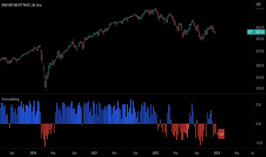
TechnicalRating█ OVERVIEW
This library is a Pine Script™ programmer’s tool for incorporating TradingView's well-known technical ratings within their scripts. The ratings produced by this library are the same as those from the speedometers in the technical analysis summary and the "Rating" indicator in the Screener , which use the aggregate biases of 26 technical indicators to calculate their results.
█ CONCEPTS
Ensemble analysis
Ensemble analysis uses multiple weaker models to produce a potentially stronger one. A common form of ensemble analysis in technical analysis is the usage of aggregate indicators together in hopes of gaining further market insight and reinforcing trading decisions.
Technical ratings
Technical ratings provide a simplified way to analyze financial markets by combining signals from an ensemble of indicators into a singular value, allowing traders to assess market sentiment more quickly and conveniently than analyzing each constituent separately. By consolidating the signals from multiple indicators into a single rating, traders can more intuitively and easily interpret the "technical health" of the market.
Calculating the rating value
Using a variety of built-in TA functions and functions from our ta library, this script calculates technical ratings for moving averages, oscillators, and their overall result within the `calcRatingAll()` function.
The function uses the script's `calcRatingMA()` function to calculate the moving average technical rating from an ensemble of 15 moving averages and filters:
• Six Simple Moving Averages and six Exponential Moving Averages with periods of 10, 20, 30, 50, 100, and 200
• A Hull Moving Average with a period of 9
• A Volume-Weighted Moving Average with a period of 20
• An Ichimoku Cloud with a conversion line length of 9, base length of 26, and leading span B length of 52
The function uses the script's `calcRating()` function to calculate the oscillator technical rating from an ensemble of 11 oscillators:
• RSI with a period of 14
• Stochastic with a %K period of 14, a smoothing period of 3, and a %D period of 3
• CCI with a period of 20
• ADX with a DI length of 14 and an ADX smoothing period of 14
• Awesome Oscillator
• Momentum with a period of 10
• MACD with fast, slow, and signal periods of 12, 26, and 9
• Stochastic RSI with an RSI period of 14, a %K period of 14, a smoothing period of 3, and a %D period of 3
• Williams %R with a period of 14
• Bull Bear Power with a period of 50
• Ultimate Oscillator with fast, middle, and slow lengths of 7, 14, and 28
Each indicator is assigned a value of +1, 0, or -1, representing a bullish, neutral, or bearish rating. The moving average rating is the mean of all ratings that use the `calcRatingMA()` function, and the oscillator rating is the mean of all ratings that use the `calcRating()` function. The overall rating is the mean of the moving average and oscillator ratings, which ranges between +1 and -1. This overall rating, along with the separate MA and oscillator ratings, can be used to gain insight into the technical strength of the market. For a more detailed breakdown of the signals and conditions used to calculate the indicators' ratings, consult our Help Center explanation.
Determining rating status
The `ratingStatus()` function produces a string representing the status of a series of ratings. The `strongBound` and `weakBound` parameters, with respective default values of 0.5 and 0.1, define the bounds for "strong" and "weak" ratings.
The rating status is determined as follows:
Rating Value Rating Status
< -strongBound Strong Sell
< -weakBound Sell
-weakBound to weakBound Neutral
> weakBound Buy
> strongBound Strong Buy
By customizing the `strongBound` and `weakBound` values, traders can tailor the `ratingStatus()` function to fit their trading style or strategy, leading to a more personalized approach to evaluating ratings.
Look first. Then leap.
█ FUNCTIONS
This library contains the following functions:
calcRatingAll()
Calculates 3 ratings (ratings total, MA ratings, indicator ratings) using the aggregate biases of 26 different technical indicators.
Returns: A 3-element tuple: ( [(float) ratingTotal, (float) ratingOther, (float) ratingMA ].
countRising(plot)
Calculates the number of times the values in the given series increase in value up to a maximum count of 5.
Parameters:
plot : (series float) The series of values to check for rising values.
Returns: (int) The number of times the values in the series increased in value.
ratingStatus(ratingValue, strongBound, weakBound)
Determines the rating status of a given series based on its values and defined bounds.
Parameters:
ratingValue : (series float) The series of values to determine the rating status for.
strongBound : (series float) The upper bound for a "strong" rating.
weakBound : (series float) The upper bound for a "weak" rating.
Returns: (string) The rating status of the given series ("Strong Buy", "Buy", "Neutral", "Sell", or "Strong Sell").
Statistics
Signal AnalyzerThis library contains functions that try to analyze trading signals performance.
Like the % of average returns after a long or short signal is provided or the number of times that signal was correct, in the inmediate 2 candles after the signal.

Hurst Exponent (Dubuc's variation method)Library "Hurst"
hurst(length, samples, hi, lo)
Estimate the Hurst Exponent using Dubuc's variation method
Parameters:
length : The length of the history window to use. Large values do not cause lag.
samples : The number of scale samples to take within the window. These samples are then used for regression. The minimum value is 2 but 3+ is recommended. Large values give more accurate results but suffer from a performance penalty.
hi : The high value of the series to analyze.
lo : The low value of the series to analyze.
The Hurst Exponent is a measure of fractal dimension, and in the context of time series it may be interpreted as indicating a mean-reverting market if the value is below 0.5 or a trending market if the value is above 0.5. A value of exactly 0.5 corresponds to a random walk.
There are many definitions of fractal dimension and many methods for its estimation. Approaches relying on calculation of an area, such as the Box Counting Method, are inappropriate for time series data, because the units of the x-axis (time) do match the units of the y-axis (price). Other approaches such as Detrended Fluctuation Analysis are useful for nonstationary time series but are not exactly equivalent to the Hurst Exponent.
This library implements Dubuc's variation method for estimating the Hurst Exponent. The technique is insensitive to x-axis units and is therefore useful for time series. It will give slightly different results to DFA, and the two methods should be compared to see which estimator fits your trading objectives best.
Original Paper:
Dubuc B, Quiniou JF, Roques-Carmes C, Tricot C. Evaluating the fractal dimension of profiles. Physical Review A. 1989;39(3):1500-1512. DOI: 10.1103/PhysRevA.39.1500
Review of various Hurst Exponent estimators for time-series data, including Dubuc's method:
www.intechopen.com

NetLiquidityLibraryLibrary "NetLiquidityLibrary"
The Net Liquidity Library provides daily values for net liquidity. Net liquidity is measured as Fed Balance Sheet - Treasury General Account - Reverse Repo. Time series for each individual component included too.
get_net_liquidity_for_date(t)
Function takes date in timestamp form and returns the Net Liquidity value for that date. If date is not present, 0 is returned.
Parameters:
t : The timestamp of the date you are requesting the Net Liquidity value for.
Returns: The Net Liquidity value for the specified date.
get_net_liquidity()
Gets the Net Liquidity time series from Dec. 2021 to current. Dates that are not present are represented as 0.
Returns: The Net Liquidity time series.

ReduceSecurityCallsLibrary "ReduceSecurityCalls"
This library allows you to reduce the number of request.security calls to 1 per symbol per timeframe. Script provides example how to use it with request.security and possible optimisation applied to htf data call.
This data can be used to calculate everything you need and more than that (for example you can calculate 4 emas with one function call on mat_out).
ParseSource(mat_outs, o)
Should be used inside request.security call. Optimise your calls using timeframe.change when htf data parsing! Supports up to 5 expressions (results of expressions must be float or int)
Parameters:
mat_outs : Matrix to be used as outputs, first value is newest
o : Please use parametres in the order they specified (o should be 1st, h should be 2nd etc..)
Returns: outs array, due to weird limitations do not try this :matrix_out = matrix.copy(ParseSource)

kNNLibrary "kNN"
Collection of experimental kNN functions. This is a work in progress, an improvement upon my original kNN script:
The script can be recreated with this library. Unlike the original script, that used multiple arrays, this has been reworked with the new Pine Script matrix features.
To make a kNN prediction, the following data should be supplied to the wrapper:
kNN : filter type. Right now either Binary or Percent . Binary works like in the original script: the system stores whether the price has increased (+1) or decreased (-1) since the previous knnStore event (called when either long or short condition is supplied). Percent works the same, but the values stored are the difference of prices in percents. That way larger differences in prices would give higher scores.
k : number k. This is how many nearest neighbors are to be selected (and summed up to get the result).
skew : kNN minimum difference. Normally, the prediction is done with a simple majority of the neighbor votes. If skew is given, then more than a simple majority is needed for a prediction. This also means that there are inputs for which no prediction would be given (if the majority votes are between -skew and +skew). Note that in Percent mode more profitable trades will have higher voting power.
depth : kNN matrix size limit. Originally, the whole available history of trades was used to make a prediction. This not only requires more computational power, but also neglects the fact that the market conditions are changing. This setting restricts the memory matrix to a finite number of past trades.
price : price series
long : long condition. True if the long conditions are met, but filters are not yet applied. For example, in my original script, trades are only made on crossings of fast and slow MAs. So, whenever it is possible to go long, this value is set true. False otherwise.
short : short condition. Same as long , but for short condition.
store : whether the inputs should be stored. Additional filters may be applied to prevent bad trades (for example, trend-based filters), so if you only need to consult kNN without storing the trade, this should be set to false.
feature1 : current value of feature 1. A feature in this case is some kind of data derived from the price. Different features may be used to analyse the price series. For example, oscillator values. Not all of them may be used for kNN prediction. As the current kNN implementation is 2-dimensional, only two features can be used.
feature2 : current value of feature 2.
The wrapper returns a tuple: [ longOK, shortOK ]. This is a pair of filters. When longOK is true, then kNN predicts a long trade may be taken. When shortOK is true, then kNN predicts a short trade may be taken. The kNN filters are returned whenever long or short conditions are met. The trade is supposed to happen when long or short conditions are met and when the kNN filter for the desired direction is true.
Exported functions :
knnStore(knn, p1, p2, src, maxrows)
Store the previous trade; buffer the current one until results are in. Results are binary: up/down
Parameters:
knn : knn matrix
p1 : feature 1 value
p2 : feature 2 value
src : current price
maxrows : limit the matrix size to this number of rows (0 of no limit)
Returns: modified knn matrix
knnStorePercent(knn, p1, p2, src, maxrows)
Store the previous trade; buffer the current one until results are in. Results are in percents
Parameters:
knn : knn matrix
p1 : feature 1 value
p2 : feature 2 value
src : current price
maxrows : limit the matrix size to this number of rows (0 of no limit)
Returns: modified knn matrix
knnGet(distance, result)
Get neighbours by getting k results with the smallest distances
Parameters:
distance : distance array
result : result array
Returns: array slice of k results
knnDistance(knn, p1, p2)
Create a distance array from the two given parameters
Parameters:
knn : knn matrix
p1 : feature 1 value
p2 : feature 2 value
Returns: distance array
knnSum(knn, p1, p2, k)
Make a prediction, finding k nearest neighbours and summing them up
Parameters:
knn : knn matrix
p1 : feature 1 value
p2 : feature 2 value
k : sum k nearest neighbors
Returns: sum of k nearest neighbors
doKNN(kNN, k, skew, depth, price, long, short, store, feature1, feature2)
execute kNN filter
Parameters:
kNN : filter type
k : number k
skew : kNN minimum difference
depth : kNN matrix size limit
price : series
long : long condition
short : short condition
store : store the supplied features (if false, only checks the results without storage)
feature1 : feature 1 value
feature2 : feature 2 value
Returns: filter output

LibIndicadoresUteisLibrary "LibIndicadoresUteis"
Collection of useful indicators. This collection does not do any type of plotting on the graph, as the methods implemented can and should be used to get the return of mathematical formulas, in a way that speeds up the development of new scripts. The current version contains methods for stochastic return, slow stochastic, IFR, leverage calculation for B3 futures market, leverage calculation for B3 stock market, bollinger bands and the range of change.
estocastico(PeriodoEstocastico)
Returns the value of stochastic
Parameters:
PeriodoEstocastico : Period for calculation basis
Returns: Float with the stochastic value of the period
estocasticoLento(PeriodoEstocastico, PeriodoMedia)
Returns the value of slow stochastic
Parameters:
PeriodoEstocastico : Stochastic period for calculation basis
PeriodoMedia : Average period for calculation basis
Returns: Float with the value of the slow stochastic of the period
ifrInvenenado(PeriodoIFR, OrigemIFR)
Returns the value of the RSI/IFR Poisoned of Guima
Parameters:
PeriodoIFR : RSI/IFR period for calculation basis
OrigemIFR : Source of RSI/IFR for calculation basis
Returns: Float with the RSI/IFR value for the period
calculoAlavancagemFuturos(margem, alavancagemMaxima)
Returns the number of contracts to work based on margin
Parameters:
margem : Margin for contract unit
alavancagemMaxima : Maximum number of contracts to work
Returns: Integer with the number of contracts suggested for trading
calculoAlavancagemAcoes(alavancagemMaxima)
Returns the number of batches to work based on the margin
Parameters:
alavancagemMaxima : Maximum number of batches to work
Returns: Integer with the amount of lots suggested for trading
bandasBollinger(periodoBB, origemBB, desvioPadrao)
Returns the value of bollinger bands
Parameters:
periodoBB : Period of bollinger bands for calculation basis
origemBB : Origin of bollinger bands for calculation basis
desvioPadrao : Standard Deviation of bollinger bands for calculation basis
Returns: Two-position array with upper and lower band values respectively
theRoc(periodoROC, origemROC)
Returns the value of Rate Of Change
Parameters:
periodoROC : Period for calculation basis
origemROC : Source of calculation basis
Returns: Float with the value of Rate Of Change
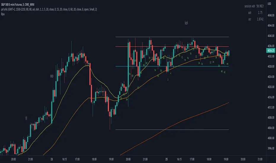
BpaLibrary "Bpa"
TODO: library of Brooks Price Action concepts
isBreakoutBar(atr, high, low, close, open, tail, size)
TODO: check if the bar is a breakout based on the specified conditions
Parameters:
atr : TODO: atr value
high : TODO: high price
low : TODO: low price
close : TODO: close price
open : TODO: open price
tail : TODO: decimal value for a percent that represent the size of the tail of the bar that cant be preceeded to be considered strong close
size : TODO: decimal value for a percent that represents by how much the breakout bar should be bigger than others to be considered one
Returns: TODO: boolean value, true if breakout bar, false otherwise
LibraryCOTLibrary "LibraryCOT"
This library provides tools to help Pine programmers fetch Commitment of Traders (COT) data for futures.
rootToCFTCCode(root)
Accepts a futures root and returns the relevant CFTC code.
Parameters:
root : Root prefix of the future's symbol, e.g. "ZC" for "ZC1!"" or "ZCU2021".
Returns: The part of a COT ticker corresponding to `root`, or "" if no CFTC code exists for the `root`.
currencyToCFTCCode(curr)
Converts a currency string to its corresponding CFTC code.
Parameters:
curr : Currency code, e.g., "USD" for US Dollar.
Returns: The corresponding to the currency, if one exists.
optionsToTicker(includeOptions)
Returns the part of a COT ticker using the `includeOptions` value supplied, which determines whether options data is to be included.
Parameters:
includeOptions : A "bool" value: 'true' if the symbol should include options and 'false' otherwise.
Returns: The part of a COT ticker: "FO" for data that includes options and "F" for data that doesn't.
metricNameAndDirectionToTicker(metricName, metricDirection)
Returns a string corresponding to a metric name and direction, which is one component required to build a valid COT ticker ID.
Parameters:
metricName : One of the metric names listed in this library's chart. Invalid values will cause a runtime error.
metricDirection : Metric direction. Possible values are: "Long", "Short", "Spreading", and "No direction". Valid values vary with metrics. Invalid values will cause a runtime error.
Returns: The part of a COT ticker ID string, e.g., "OI_OLD" for "Open Interest" and "No direction", or "TC_L" for "Traders Commercial" and "Long".
typeToTicker(metricType)
Converts a metric type into one component required to build a valid COT ticker ID. See the "Old and Other Futures" section of the CFTC's Explanatory Notes for details on types.
Parameters:
metricType : Metric type. Accepted values are: "All", "Old", "Other".
Returns: The part of a COT ticker.
convertRootToCOTCode(mode, convertToCOT)
Depending on the `mode`, returns a CFTC code using the chart's symbol or its currency information when `convertToCOT = true`. Otherwise, returns the symbol's root or currency information. If no COT data exists, a runtime error is generated.
Parameters:
mode : A string determining how the function will work. Valid values are:
"Root": the function extracts the futures symbol root (e.g. "ES" in "ESH2020") and looks for its CFTC code.
"Base currency": the function extracts the first currency in a pair (e.g. "EUR" in "EURUSD") and looks for its CFTC code.
"Currency": the function extracts the quote currency ("JPY" for "TSE:9984" or "USDJPY") and looks for its CFTC code.
"Auto": the function tries the first three modes (Root -> Base Currency -> Currency) until a match is found.
convertToCOT : "bool" value that, when `true`, causes the function to return a CFTC code. Otherwise, the root or currency information is returned. Optional. The default is `true`.
Returns: If `convertToCOT` is `true`, the part of a COT ticker ID string. If `convertToCOT` is `false`, the root or currency extracted from the current symbol.
COTTickerid(COTType, CTFCCode, includeOptions, metricName, metricDirection, metricType)
Returns a valid TradingView ticker for the COT symbol with specified parameters.
Parameters:
COTType : A string with the type of the report requested with the ticker, one of the following: "Legacy", "Disaggregated", "Financial".
CTFCCode : The for the asset, e.g., wheat futures (root "ZW") have the code "001602".
includeOptions : A boolean value. 'true' if the symbol should include options and 'false' otherwise.
metricName : One of the metric names listed in this library's chart.
metricDirection : Direction of the metric, one of the following: "Long", "Short", "Spreading", "No direction".
metricType : Type of the metric. Possible values: "All", "Old", and "Other".
Returns: A ticker ID string usable with `request.security()` to fetch the specified Commitment of Traders data.

TradingWolfLibaryLibrary "TradingWolfLibary"
getMA(int, string)
Gets a Moving Average based on type
Parameters:
int : length The MA period
string : maType The type of MA
Returns: A moving average with the given parameters
minStop(float, simple, float, string)
Calculates and returns Minimum stop loss
Parameters:
float : entry price (Close if calculating on the entry candle)
simple : int Calculate how many bars back to look at swings
float : Minimum Stop Loss allowed (Should be x 0.01) if input
string : Direciton of trade either "Long" or "Short"
Returns: Stop Loss Value

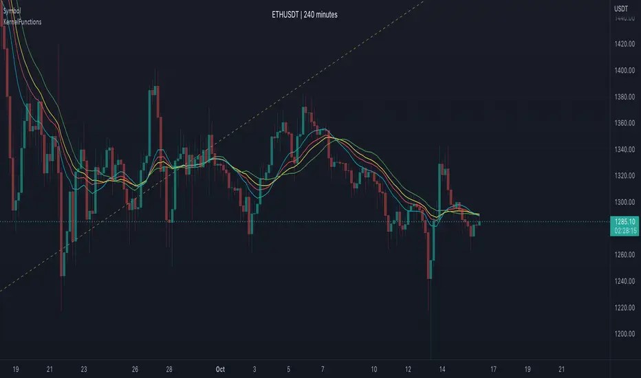
KernelFunctionsLibrary "KernelFunctions"
This library provides non-repainting kernel functions for Nadaraya-Watson estimator implementations. This allows for easy substitution/comparison of different kernel functions for one another in indicators. Furthermore, kernels can easily be combined with other kernels to create newer, more customized kernels. Compared to Moving Averages (which are really just simple kernels themselves), these kernel functions are more adaptive and afford the user an unprecedented degree of customization and flexibility.
rationalQuadratic(_src, _lookback, _relativeWeight, _startAtBar)
Rational Quadratic Kernel - An infinite sum of Gaussian Kernels of different length scales.
Parameters:
_src : The source series.
_lookback : The number of bars used for the estimation. This is a sliding value that represents the most recent historical bars.
_relativeWeight : Relative weighting of time frames. Smaller values result in a more stretched-out curve, and larger values will result in a more wiggly curve. As this value approaches zero, the longer time frames will exert more influence on the estimation. As this value approaches infinity, the behavior of the Rational Quadratic Kernel will become identical to the Gaussian kernel.
_startAtBar : Bar index on which to start regression. The first bars of a chart are often highly volatile, and omitting these initial bars often leads to a better overall fit.
Returns: yhat The estimated values according to the Rational Quadratic Kernel.
gaussian(_src, _lookback, _startAtBar)
Gaussian Kernel - A weighted average of the source series. The weights are determined by the Radial Basis Function (RBF).
Parameters:
_src : The source series.
_lookback : The number of bars used for the estimation. This is a sliding value that represents the most recent historical bars.
_startAtBar : Bar index on which to start regression. The first bars of a chart are often highly volatile, and omitting these initial bars often leads to a better overall fit.
Returns: yhat The estimated values according to the Gaussian Kernel.
periodic(_src, _lookback, _period, _startAtBar)
Periodic Kernel - The periodic kernel (derived by David Mackay) allows one to model functions that repeat themselves exactly.
Parameters:
_src : The source series.
_lookback : The number of bars used for the estimation. This is a sliding value that represents the most recent historical bars.
_period : The distance between repititions of the function.
_startAtBar : Bar index on which to start regression. The first bars of a chart are often highly volatile, and omitting these initial bars often leads to a better overall fit.
Returns: yhat The estimated values according to the Periodic Kernel.
locallyPeriodic(_src, _lookback, _period, _startAtBar)
Locally Periodic Kernel - The locally periodic kernel is a periodic function that slowly varies with time. It is the product of the Periodic Kernel and the Gaussian Kernel.
Parameters:
_src : The source series.
_lookback : The number of bars used for the estimation. This is a sliding value that represents the most recent historical bars.
_period : The distance between repititions of the function.
_startAtBar : Bar index on which to start regression. The first bars of a chart are often highly volatile, and omitting these initial bars often leads to a better overall fit.
Returns: yhat The estimated values according to the Locally Periodic Kernel.
ahpuhelperLibrary "ahpuhelper"
Helper Library for Auto Harmonic Patterns UltimateX. It is not meaningful for others. This is supposed to be private library. But, publishing it to make sure that I don't delete accidentally. Some functions may be useful for coders.
insert_open_trades_table_column(showOpenTrades, table_id, column, colors, values, intStatus, harmonicTrailingStartState, lblSizeOpenTrades)
add data to open trades table column
Parameters:
showOpenTrades : flag to show open trades table
table_id : Table Id
column : refers to pattern data
colors : backgroud and text color array
values : cell values
intStatus : status as integer
harmonicTrailingStartState : trailing Start state as per configs
lblSizeOpenTrades : text size
Returns: nextColumn
populate_closed_stats(ClosedStatsPosition, bullishCounts, bearishCounts, bullishRetouchCounts, bearishRetouchCounts, bullishSizeMatrix, bearishSizeMatrix, bullishRR, bearishRR, allPatternLabels, flags, rowMain, rowHeaders)
populate closed stats for harmonic patterns
Parameters:
ClosedStatsPosition : Table position for closed stats
bullishCounts : Matrix containing bullish trade stats
bearishCounts : Matrix containing bearish trade stats
bullishRetouchCounts : Matrix containing bullish trade stats for those which retouched entry
bearishRetouchCounts : Matrix containing bearish trade stats for those which retouched entry
bullishSizeMatrix : Matrix containing data about size of bullish patterns
bearishSizeMatrix : Matrix containing data about size of bearish patterns
bullishRR : Matrix containing Risk Reward data of bullish patterns
bearishRR : Matrix containing Risk Reward data of bearish patterns
allPatternLabels : array containing pattern labels
flags : display flags
rowMain : Pattern header data
rowHeaders : header grouping data
Returns: void
get_rr_details(patternTradeDetails, harmonicTrailingStartState, disableTrail, breakEvenTrail)
calculate and return risk reward based on targets and stops
Parameters:
patternTradeDetails : array containing stop, entry and targets
harmonicTrailingStartState : trailing point
disableTrail : If set, ignores trailing point
breakEvenTrail : If set, trailing does not go beyond breakeven.
Returns: nextColumn

normsinvLibrary "normsinv"
Description:
Returns the inverse of the standard normal cumulative distribution.
The distribution has a mean of zero and a standard deviation of one; i.e.,
normsinv seeks that value z such that a normal distribtuion of mean of zero
and standard deviation one is equal to the input probability.
Reference:
github.com
normsinv(y0)
Returns the inverse of the standard normal cumulative distribution. The distribution has a mean of zero and a standard deviation of one.
Parameters:
y0 : float, probability corresponding to the normal distribution.
Returns: float, z-score
cndevLibrary "cndev"
This function returns the inverse of cumulative normal distribution function
Reference:
The Full Monte, by Boris Moro, Union Bank of Switzerland . RISK 1995(2)
CNDEV(U)
Returns the inverse of cumulative normal distribution function
Parameters:
U : float,
Returns: float.
Strategy PnL LibraryLibrary "Strategy_PnL_Library"
TODO: This is a library that helps you learn current pnl of open position and use it to create your own dynamic take profit or stop loss rules based on current level of your profit. It should only be used with strategies.
inTrade()
inTrade: Checks if a position is currently open.
Returns: bool: true for yes, false for no.
notInTrade()
inTrade: Checks if a position is currently open. Interchangeable with inTrade but just here for simple semantics.
Returns: bool: true for yes, false for no.
pnl()
pnl: Calculates current profit or loss of position after the commission. If the strategy is not in trade it will always return na.
Returns: float: Current Profit or Loss of position, positive values for profit, negative values for loss.
entryBars()
entryBars: Checks how many bars it's been since the entry of the position.
Returns: int: Returns a int of strategy entry bars back. Minimum value is always corrected to 1 to avoid lookback errors.
pnlvelocity()
pnlvelocity: Calculates the velocity of pnl by following the change in open profit compared to previous bar. If the strategy is not in trade it will always return na.
Returns: float: Returns a float value of pnl velocity.
pnlacc()
pnlacc: Calculates the acceleration of pnl by following the change in profit velocity compared to previous bar. If the strategy is not in trade it will always return na.
Returns: float: Returns a float value of pnl acceleration.
pnljerk()
pnljerk: Calculates the jerk of pnl by following the change in profit acceleration compared to previous bar. If the strategy is not in trade it will always return na.
Returns: float: Returns a float value of pnl jerk.
pnlhigh()
pnlhigh: Calculates the highest value the pnl has reached since the start of the current position. If the strategy is not in trade it will always return na.
Returns: float: Returns a float highest value the pnl has reached.
pnllow()
pnllow: Calculates the lowest value the pnl has reached since the start of the current position. If the strategy is not in trade it will always return na.
Returns: float: Returns a float lowest value the pnl has reached.
pnldev()
pnldev: Calculates the deviance of the pnl since the start of the current position. If the strategy is not in trade it will always return na.
Returns: float: Returns a float deviance value of the pnl.
pnlvar()
pnlvar: Calculates the variance value of the pnl since the start of the current position. If the strategy is not in trade it will always return na.
Returns: float: Returns a float variance value of the pnl.
pnlstdev()
pnlstdev: Calculates the stdev value of the pnl since the start of the current position. If the strategy is not in trade it will always return na.
Returns: float: Returns a float stdev value of the pnl.
pnlmedian()
pnlmedian: Calculates the median value of the pnl since the start of the current position. If the strategy is not in trade it will always return na.
Returns: float: Returns a float median value of the pnl.
ctndLibrary "ctnd"
Description:
Double precision algorithm to compute the cumulative trivariate normal distribution
found in A.Genz, Numerical computation of rectangular bivariate and trivariate normal
and t probabilities”, Statistics and Computing, 14, (3), 2004. The cumulative trivariate
normal is needed to price window barrier options, see G.F. Armstrong, Valuation formulae
or window barrier options”, Applied Mathematical Finance, 8, 2001.
References:
link.springer.com
www.tandfonline.com
citeseerx.ist.psu.edu
The Complete Guide to Option Pricing Formulas, 2nd ed. (Espen Gaarder Haug)
CTND(LIMIT1, LIMIT2, LIMIT3, SIGMA1, SIGMA2, SIGMA3)
Returns the Cumulative Trivariate Normal Distribution
Parameters:
LIMIT1 : float,
LIMIT2 : float,
LIMIT3 : float,
SIGMA1 : float,
SIGMA2 : float,
SIGMA3 : float,
Returns: float.

combinLibrary "combin"
Description:
The combin function is a the combination function
as it calculates the number of possible combinations for two given numbers.
This function takes two arguments: the number and the number_chosen.
For example, if the number is 5 and the number chosen is 1,
there are 5 combinations, giving 5 as a result.
Reference:
ideone.com
support.microsoft.com
combin(n, kin)
Returns the number of combinations for a given number of items. Use to determine the total possible number of groups for a given number of items.
Parameters:
n : int, The number of items.
kin : int, The number of items in each combination.
Returns: int.

norminvLibrary "norminv"
Description:
An inverse normal distribution is a way to work backwards
from a known probability to find an x-value. It is an informal term and
doesn't refer to a particular probability distribution. Returns the
value of the inverse normal distribution function for a specified value,
mean, and standard deviation.
Reference:
github.com
support.microsoft.com
norminv(x, mean, stdev)
Returns the value of the inverse normal distribution function for a specified value, mean, and standard deviation.
Parameters:
x : float, The input to the normal distribution function.
mean : float, The mean (mu) of the normal distribution function
stdev : float, The standard deviation (sigma) of the normal distribution function.
Returns: float.

cbndLibrary "cbnd"
Description:
A standalone Cumulative Bivariate Normal Distribution (CBND) functions that do not require any external libraries.
This includes 3 different CBND calculations: Drezner(1978), Drezner and Wesolowsky (1990), and Genz (2004)
Comments:
The standardized cumulative normal distribution function returns the probability that one random
variable is less than a and that a second random variable is less than b when the correlation
between the two variables is p. Since no closed-form solution exists for the bivariate cumulative
normal distribution, we present three approximations. The first one is the well-known
Drezner (1978) algorithm. The second one is the more efficient Drezner and Wesolowsky (1990)
algorithm. The third is the Genz (2004) algorithm, which is the most accurate one and therefore
our recommended algorithm. West (2005b) and Agca and Chance (2003) discuss the speed and
accuracy of bivariate normal distribution approximations for use in option pricing in
ore detail.
Reference:
The Complete Guide to Option Pricing Formulas, 2nd ed. (Espen Gaarder Haug)
CBND1(A, b, rho)
Returns the Cumulative Bivariate Normal Distribution (CBND) using Drezner 1978 Algorithm
Parameters:
A : float,
b : float,
rho : float,
Returns: float.
CBND2(A, b, rho)
Returns the Cumulative Bivariate Normal Distribution (CBND) using Drezner and Wesolowsky (1990) function
Parameters:
A : float,
b : float,
rho : float,
Returns: float.
CBND3(x, y, rho)
Returns the Cumulative Bivariate Normal Distribution (CBND) using Genz (2004) algorithm (this is the preferred method)
Parameters:
x : float,
y : float,
rho : float,
Returns: float.
cndLibrary "cnd"
Cumulative Normal Distribution
CND1(x)
Returns the Cumulative Normal Distribution (CND) using the Hart (1968) method. (preferred method, 14-18 decimal accuracy)
Parameters:
x : float,
Returns: float.
CND2(x)
Returns the Cumulative Normal Distribution (CND) using the Abromowitz and Stegun (1974) Polynomial Approximation.
Parameters:
x : float,
Returns: float.
CND3(x)
Returns the Cumulative Normal Distribution (CND) using Newton-Cotes method, Boole’s rule
Parameters:
x : float,
Returns: float.
chi2InvLibrary "chi2Inv"
chi2Inv(p, n)
Returns the inverse cumulative distribution function (icdf) of the chi-square distribution with degrees of freedom nu, evaluated at the probability values in p. Goldstein approximation
Parameters:
p : float, probability
n : float, degress of freedom source.
Returns: float.
TradersCustomLibraryLibrary "TradersCustomLibrary"
TODO: add library description here
SelectOptimalTimeframeTrendlineSettings()
calculateShortStopLoss()
calculateLongStopLoss()
werdygerTrend()
trendLines()
stoch()
timeToString()
TALibrary "TA"
General technical analysis functions
div_bull(pS, iS, cp_length_after, cp_length_before, pivot_length, lookback, no_broken, pW, iW, hidW, regW)
Test for bullish divergence
Parameters:
pS : Price series (float)
iS : Indicator series (float)
cp_length_after : Bars after current (divergent) pivot low to be considered a valid pivot (optional int)
cp_length_before : Bars before current (divergent) pivot low to be considered a valid pivot (optional int)
pivot_length : Bars before and after prior pivot low to be considered valid pivot (optional int)
lookback : Bars back to search for prior pivot low (optional int)
no_broken : Flag to only consider divergence valid if the pivot-to-pivot trendline is unbroken (optional bool)
pW : Weight of change in price, used in degree of divergence calculation (optional float)
iW : Weight of change in indicator, used in degree of divergence calculation (optional float)
hidW : Weight of hidden divergence, used in degree of divergence calculation (optional float)
regW : Weight of regular divergence, used in degree of divergence calculation (optional float)
Returns:
flag = true if divergence exists (bool)
degree = degree (strength) of divergence (float)
type = 1 = regular, 2 = hidden (int)
lx1 = x coordinate 1 (int)
ly1 = y coordinate 1 (float)
lx2 = x coordinate 2 (int)
ly2 = y coordinate 2 (float)
div_bear(pS, iS, cp_length_after, cp_length_before, pivot_length, lookback, no_broken, pW, iW, hidW, regW)
Test for bearish divergence
Parameters:
pS : Price series (float)
iS : Indicator series (float)
cp_length_after : Bars after current (divergent) pivot high to be considered a valid pivot (optional int)
cp_length_before : Bars before current (divergent) pivot highto be considered a valid pivot (optional int)
pivot_length : Bars before and after prior pivot high to be considered valid pivot (optional int)
lookback : Bars back to search for prior pivot high (optional int)
no_broken : Flag to only consider divergence valid if the pivot-to-pivot trendline is unbroken (optional bool)
pW : Weight of change in price, used in degree of divergence calculation (optional float)
iW : Weight of change in indicator, used in degree of divergence calculation (optional float)
hidW : Weight of hidden divergence, used in degree of divergence calculation (optional float)
regW : Weight of regular divergence, used in degree of divergence calculation (optional float)
Returns:
flag = true if divergence exists (bool)
degree = degree (strength) of divergence (float)
type = 1 = regular, 2 = hidden (int)
lx1 = x coordinate 1 (int)
ly1 = y coordinate 1 (float)
lx2 = x coordinate 2 (int)
ly2 = y coordinate 2 (float)
