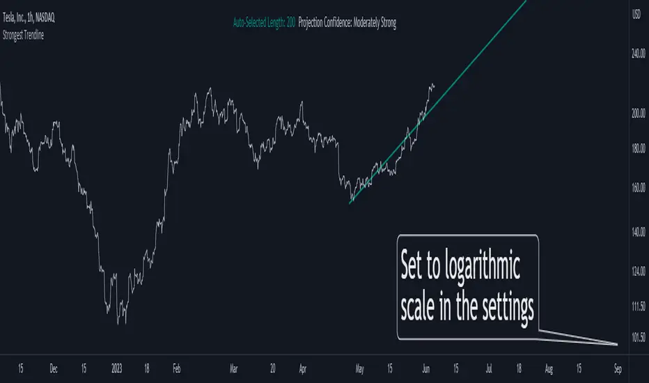
Strongest TrendlineUnleashing the Power of Trendlines with the "Strongest Trendline" Indicator.
Trendlines are an invaluable tool in technical analysis, providing traders with insights into price movements and market trends. The "Strongest Trendline" indicator offers a powerful approach to identifying robust trendlines based on various parameters and technical analysis metrics.
When using the "Strongest Trendline" indicator, it is recommended to utilize a logarithmic scale . This scale accurately represents percentage changes in price, allowing for a more comprehensive visualization of trends. Logarithmic scales highlight the proportional relationship between prices, ensuring that both large and small price movements are given due consideration.
One of the notable advantages of logarithmic scales is their ability to balance price movements on a chart. This prevents larger price changes from dominating the visual representation, providing a more balanced perspective on the overall trend. Logarithmic scales are particularly useful when analyzing assets with significant price fluctuations.
In some cases, traders may need to scroll back on the chart to view the trendlines generated by the "Strongest Trendline" indicator. By scrolling back, traders ensure they have a sufficient historical context to accurately assess the strength and reliability of the trendline. This comprehensive analysis allows for the identification of trendline patterns and correlations between historical price movements and current market conditions.
The "Strongest Trendline" indicator calculates trendlines based on historical data, requiring an adequate number of data points to identify the strongest trend. By scrolling back and considering historical patterns, traders can make more informed trading decisions and identify potential entry or exit points.
When using the "Strongest Trendline" indicator, a higher Pearson's R value signifies a stronger trendline. The closer the Pearson's R value is to 1, the more reliable and robust the trendline is considered to be.
In conclusion, the "Strongest Trendline" indicator offers traders a robust method for identifying trendlines with significant predictive power. By utilizing a logarithmic scale and considering historical data, traders can unleash the full potential of this indicator and gain valuable insights into price trends. Trendlines, when used in conjunction with other technical analysis tools, can help traders make more informed decisions in the dynamic world of financial markets.
Bands
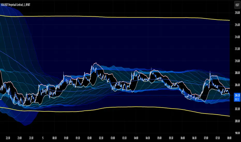
TrueLevel BandsTrueLevel Bands is a powerful trading indicator that employs linear regression and standard deviation to create dynamic, envelope-style bands around the price action of a financial instrument. These bands are designed to help traders identify potential support and resistance levels, trend direction, and volatility.
The TrueLevel Bands indicator consists of multiple envelope bands, each constructed using different timeframes or lengths, and a multiple (mult) factor. The multiple factor determines the width of the bands by adjusting the number of standard deviations from the linear regression line.
Key Features of TrueLevel Bands
1. Multi-Timeframe Analysis: Unlike traditional moving average-based indicators, TrueLevel Bands allow traders to incorporate multiple timeframes into their analysis. This helps traders capture both short-term and long-term market dynamics, offering a more comprehensive understanding of price behavior.
2. Customization: The TrueLevel Bands indicator offers a high level of customization, allowing traders to adjust the lengths and multiple factors to suit their trading style and preferences. This flexibility enables traders to fine-tune the indicator to work optimally with various instruments and market conditions.
3. Adaptive Volatility: By incorporating standard deviation, TrueLevel Bands can automatically adjust to changing market volatility. This feature enables the bands to expand during periods of high volatility and contract during periods of low volatility, providing traders with a more accurate representation of market dynamics.
4. Dynamic Support and Resistance Levels: TrueLevel Bands can help traders identify dynamic support and resistance levels, as the bands adjust in real-time according to price action. This can be particularly useful for traders looking to enter or exit positions based on support and resistance levels.
5. The "Global Trend Line" refers to the average of the bands used to indicate the overall trend.
Why TrueLevel Bands are Different from Classic Moving Averages
TrueLevel Bands differ from conventional moving averages in several ways:
1. Linear Regression: While moving averages are based on simple arithmetic means, TrueLevel Bands use linear regression to determine the centerline. This offers a more accurate representation of the trend and helps traders better assess potential entry and exit points.
2. Envelope Style Bands: Unlike moving averages, which are single lines, TrueLevel Bands form envelope-style bands around the price action. This provides traders with a visual representation of potential support and resistance levels, trend direction, and volatility.
3. Multi-Timeframe Analysis: Classic moving averages typically focus on a single timeframe. In contrast, TrueLevel Bands incorporate multiple timeframes, enabling traders to capture a broader understanding of market dynamics.
4. Adaptive Volatility: Traditional moving averages do not account for changing market volatility, whereas TrueLevel Bands automatically adjust to volatility shifts through the use of standard deviation.
The TrueLevel Bands indicator is a powerful, versatile tool that offers traders a unique approach to technical analysis. With its ability to adapt to changing market conditions, provide multi-timeframe analysis, and dynamic support and resistance levels, TrueLevel Bands can serve as an invaluable asset to both novice and experienced traders looking to gain an edge in the markets.

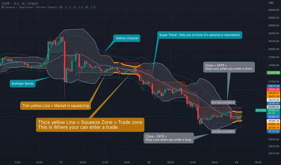
BB Squeeze + SuperTrend + Keltner ChannelBollinger Bands and Keltner Channel are two of my favorite channels. When you use them correctly, they can bring great help to your trading.
I like to use Bollinger Bands and Keltner Channels to identify when you can trade and when you can not trade, which is also known as the "squeeze".
When the opening of the Bollinger Bands is very small, it is a range that you can enter a trade, the range is called "Squeeze Zone" or "Trade zone".
When the opening of the Bollinger Bands is very large, it is a range that you cannot enter a trade, because the market fluctuates big when BB's opening is large.
I use two ways to identify when the Bollinger Bands's opening is very small or large, one is the Bollinger Bands entering Keltner Bands and one is using specific ATR ranges,. The first one allows you to identify when the market is squeezing and the second one allows you to identify when the market has entered Squeeze zone, that is, the market is already in a trading range suitable for entering a trade.(see chart.)
When the market is squeezed and you enter the trade, you can also use ATR as the stop loss price of the trade, I recommend using 2 ATR as your stop loss, and I also display them on the chart (see chart).
In addition, I also added SuperTrend to this indicator. SuperTrend is a very suitable for identifying trends. You can use SuperTrend to help you identify whether to go long or short.
This is how I use this indicator(See chart):
1.Only trade when market is in Squeeze Zone. (Thick yellow line in chart)
2.When entry a trade, use 2 ATR as stop loss. (Label in Chart)
3.Use Super trend to know to go long or short.
4.Keltner Channel helps to know when the market is squeezing. (Thin yellow line in chart.)
======== 中文說明 (Chinese Explanation) ========
Bollinger Bands(布林帶)跟 Keltner Channel(肯特納通道)是我最喜歡的兩個通道,當你正確使用它們時,它們可以替你的交易帶來非常大的幫助。
我喜歡用 Bollinger Bands 跟 Keltner Channel 來識別何時可以交易,何時不能交易,這個又稱做“擠壓操作”。當布林帶的開口很小時,便是可以交易的區間,而當布林帶的開口很大時,對我來說此時就是不可以交易的區間,因為此時市場的波動很大。
我使用兩種方式來識別當布林帶開口很小的時候,一種是布林帶進入肯特納通道,一種則使用特定的ATR範圍,前者可以讓你識別市場正在擠壓,後者則可以識別市場已經進入擠壓區間,也就是市場已經處於適合進入交易的交易區間。
當市場進入擠壓之後,而你也進入了交易,你還可以使用ATR來作為交易的止損價格,我建議使用2個ATR 來當作你的止損,而我也將他們顯示在圖表上了(見圖表)。
另外,我還在這個指標中加入了 SuperTrend(超級趨勢),SuperTrend 是一個非常適合用來辨別趨勢的指標,你可以使用 SuperTrend 來幫助你識別要做多還是做空。
這是我使用該指標的方式(見圖表):
1.僅在市場處於交易區間時進行交易。 (圖中黃色粗線)
2.入場時,使用2個ATR作為止損。 (圖表中的標籤)
3.使用超級趨勢知道做多或做空。
4.Keltner Channel 有助於了解市場何時擠壓。 (圖表中的黃色細線。)
Matrix Momentum Expansion [IkkeOmar]The indicator consists of several features:
Candlestick chart: The indicator plots a candlestick chart based on the input parameters of the user. The candlesticks are colored blue or orange depending on whether the closing price is above or below the upper and lower bands.
Support and Resistance levels: The indicator also plots support and resistance levels based on the CCI (Commodity Channel Index) of the asset's price. These levels are dynamic and change based on the user's input parameters.
Momentum: The indicator calculates the momentum of the market based on the smoothed and standard deviation of the asset's price. It uses this momentum to calculate upper and lower bands that are plotted on the chart.
Warning signals: The indicator can also be used to identify potential warning signals. When the closing price of the asset moves above the upper band, it could indicate that the market is overbought and a potential reversal could occur. Conversely, when the closing price moves below the lower band, it could indicate that the market is oversold and a potential reversal could occur.
Contractions and expansions in the bands can provide important information to traders about potential price movements.
When the bands contract, it indicates that the market is experiencing low volatility and the price is likely to move sideways. During these periods, traders may look for other signals, such as support and resistance levels or price patterns, to determine potential entry and exit points.
On the other hand, when the bands expand, it indicates that the market is experiencing high volatility and the price is likely to move in a particular direction. Traders can use this information to identify potential trend reversals or continuation patterns. When the upper and lower bands move further apart, it indicates that the trend is becoming stronger, while when they move closer together, it indicates that the trend may be weakening.
When the price moves outside of the bands, it can also provide important information to traders. If the price moves above the upper band, it could indicate that the market is overbought and a potential reversal could occur. Conversely, if the price moves below the lower band, it could indicate that the market is oversold and a potential reversal could occur.
Very important note!
When you see contractions, please understand that it's a wonderful opportunity to pivot into position to catch a good trade because we will see an expansion after!

Bollinger Bands - Breakout StrategyThe Bollinger Bands - Breakout Strategy is a trend-following optimized for short-term trading in the crypto market. This strategy employs the Bollinger Bands, a widely recognized technical indicator, as its primary instrument for pinpointing potential trades. It is capable of executing both long and short positions, depending on whether the market is in a spot or futures, and is particularly effective in trending markets.
The strategy boasts a high degree of configurability, allowing users to set the Bollinger Bands period and deviation, trend filter, volatility filter, trade direction filter, rate of change filter, and date filter. Furthermore, it offers options for Take Profit, Stop Loss, and Trailing Stop for both long and short positions, ensuring a comprehensive risk management approach. The inclusion of a maximum intraday loss feature adds another layer of protection, making this strategy a valuable tool for traders seeking a professional and adaptable trading system.
Name : Bollinger Bands - Breakout Strategy
Category : Trend Follower based on Bollinger Bands
Operating mode : Long and Short on Futures or Long on Spot
Trade duration : Intraday
Timeframe : 2H, 3H, 4H, 5H
Market : Crypto
Suggested usage : Trending Markets
Entry : When the price crosses above or below the Bollinger Bands
Exit : Opposite Cross or Profit target, Trailing stop or Stop loss
Configuration :
- Bollinger Bands period and deviation
- Trend Filter
- Volatility Filter
- Trade direction filter
- Rate of Change filter
- Date Filter (for backtesting purposes)
- Take Profit, Stop Loss and Trailing Stop for long and short positions
- Risk Management: Max Intraday Loss
Backtesting :
⁃ Exchange: BINANCE
⁃ Pair: BTCUSDT.P
⁃ Timeframe: 4H
⁃ Fee: 0.025%
⁃ Slippage: 1
- Initial Capital: 10000 USDT
- Position sizing: 10% of Equity
- Start : 2019-09-19 (Out Of Sample from 2022-12-23)
- Bar magnifier: on
Credits :
- LucF of Pine Coders for f_security function to avoid repainting using security.
- QuantNomad for Monthly Table.
Disclaimer : Risk Management is crucial, so adjust stop loss to your comfort level. A tight stop loss can help minimise potential losses. Use at your own risk.
How you or we can improve? Source code is open so share your ideas!
Leave a comment and smash the boost button!
Thanks for your attention, happy to support the TradingView community.

Bollinger Band ribbonThis indicator plots 9 upper and lower lines with increasing length. Lines are 0.618 upper and lower level of Bollinger band.
TrueLevel BandsWhat are TrueLevel Bands ?
TrueLevel Bands is a powerful trading indicator that employs linear regression and standard deviation to create dynamic, envelope-style bands around the price action of a financial instrument. These bands are designed to help traders identify potential support and resistance levels, trend direction, and volatility.
The TrueLevel Bands indicator consists of multiple envelope bands, each constructed using different timeframes or lengths, and a multiple (mult) factor. The multiple factor determines the width of the bands by adjusting the number of standard deviations from the linear regression line.
Key Features of TrueLevel Bands
1. Multi-Timeframe Analysis: Unlike traditional moving average-based indicators, TrueLevel Bands allow traders to incorporate multiple timeframes into their analysis. This helps traders capture both short-term and long-term market dynamics, offering a more comprehensive understanding of price behavior.
2. Customization: The TrueLevel Bands indicator offers a high level of customization, allowing traders to adjust the lengths and multiple factors to suit their trading style and preferences. This flexibility enables traders to fine-tune the indicator to work optimally with various instruments and market conditions.
3. Adaptive Volatility: By incorporating standard deviation, TrueLevel Bands can automatically adjust to changing market volatility. This feature enables the bands to expand during periods of high volatility and contract during periods of low volatility, providing traders with a more accurate representation of market dynamics.
4. Dynamic Support and Resistance Levels: TrueLevel Bands can help traders identify dynamic support and resistance levels, as the bands adjust in real-time according to price action. This can be particularly useful for traders looking to enter or exit positions based on support and resistance levels.
Why TrueLevel Bands are Different from Classic Moving Averages
TrueLevel Bands differ from conventional moving averages in several ways:
1. Linear Regression: While moving averages are based on simple arithmetic means, TrueLevel Bands use linear regression to determine the centerline. This offers a more accurate representation of the trend and helps traders better assess potential entry and exit points.
2. Envelope Style Bands: Unlike moving averages, which are single lines, TrueLevel Bands form envelope-style bands around the price action. This provides traders with a visual representation of potential support and resistance levels, trend direction, and volatility.
3. Multi-Timeframe Analysis: Classic moving averages typically focus on a single timeframe. In contrast, TrueLevel Bands incorporate multiple timeframes, enabling traders to capture a broader understanding of market dynamics.
4. Adaptive Volatility: Traditional moving averages do not account for changing market volatility, whereas TrueLevel Bands automatically adjust to volatility shifts through the use of standard deviation.
The TrueLevel Bands indicator is a powerful, versatile tool that offers traders a unique approach to technical analysis. With its ability to adapt to changing market conditions, provide multi-timeframe analysis, and dynamic support and resistance levels, TrueLevel Bands can serve as an invaluable asset to both novice and experienced traders looking to gain an edge in the markets.

Regression Envelope MTFThe Regression Envelope MTF indicator is a technical analysis tool that uses linear regression to identify potential price reversal points in the market. The indicator plots a linear regression line based on the selected price source over a specified length, and adds and subtracts a multiple of the standard deviation to create upper and lower bands around the line.
One advantage of using linear regression over the traditional envelope indicator is that it takes into account the slope of the trend, rather than assuming that the trend is linear. This means that the bands will adapt to the slope of the trend, which can provide more accurate signals in trending markets.
Another advantage of using linear regression over a simple moving average (SMA) is that it is less sensitive to outliers. SMAs can be heavily influenced by extreme values in the data, which can result in false signals. Linear regression, on the other hand, is more robust to outliers, which can lead to more reliable signals.
Overall, the Regression Envelope MTF indicator can be a useful tool for traders and investors looking to identify potential price reversal points and generate trading signals. However, it should be used in conjunction with other technical analysis tools and with proper risk management strategies in place.

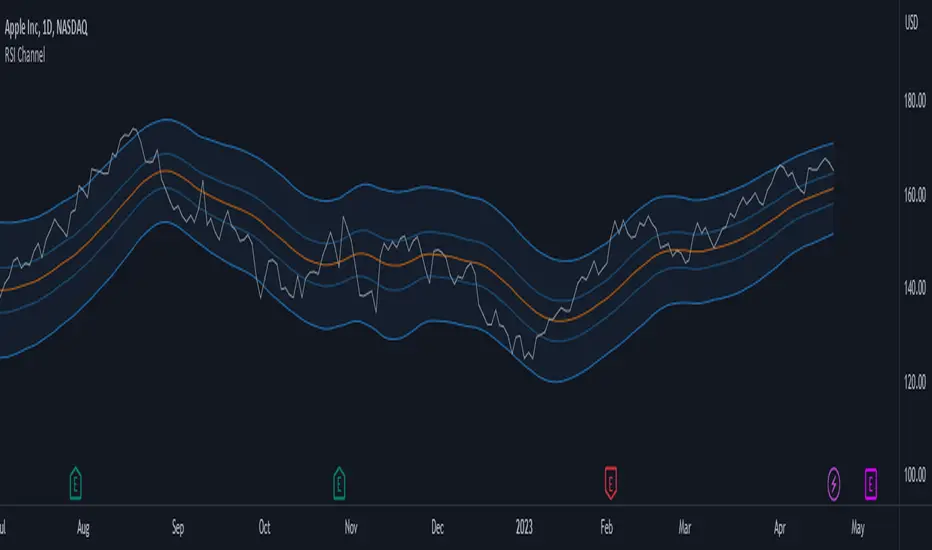
MTF RSI Channel Smoothed (Linear Regression)The "MTF RSI Channel Smoothed (Linear Regression)" indicator is a momentum oscillator that displays smoothed RSI bands across multiple timeframes.
What sets this indicator apart is that it uses linear regression to smooth the RSI bands. Linear regression is a statistical technique that helps filter out the noise in the data, resulting in smoother and more precise RSI bands. This provides traders with a more advanced and reliable tool for monitoring the RSI bands across multiple timeframes.
One of the primary advantages of using linear regression to smooth the RSI bands is that it provides a more accurate and reliable way to identify overbought and oversold levels of the asset. The linear regression method smooths out the data by reducing the impact of temporary price fluctuations, allowing traders to see the underlying trend more clearly. This helps traders to make more informed trading decisions by identifying key levels of support and resistance, and spotting potential entry and exit points.
Another advantage of the "Multi-Timeframe Smoothed RSI Bands" indicator is that it allows traders to adjust the length of the smoothing period using the "Smooth Period" parameter. This flexibility gives traders the ability to fine-tune the indicator to their specific trading style and preferences, resulting in a more personalized and effective trading tool.
Overall, the "Multi-Timeframe Smoothed RSI Bands" indicator is a powerful tool for traders looking to monitor the RSI bands across multiple timeframes. By using linear regression to smooth the data, this indicator provides traders with a more accurate and reliable way to identify potential trading opportunities, and make more informed trading decisions.
Donchian Channel Smoothed (Linear Regression)The script is an implementation of the Donchian Channel Smoothed indicator using linear regression to smooth the data. The indicator plots three curves: the middle curve, which represents the average of the upper and lower curves, and the upper and lower curves, which are the standard Donchian channels.
The smoothing is done using linear regression on the highest and lowest of the given period. This helps filter out the noise in the data and provides a smoother curve that can help traders identify trends and key levels of support and resistance. The advantages of using linear regression for smoothing are reduced data volatility, better identification of long-term trends, and improved ability to identify support and resistance levels.
Using this indicator, traders can identify potential entry and exit points in a trend, as well as key support and resistance levels. Donchian channels are also useful for measuring asset volatility and determining trading range boundaries.
In summary, using linear regression to smooth the data in the Donchian Channel Smoothed indicator presents significant advantages for traders, such as reduced data volatility and better identification of long-term trends. This allows traders to more easily identify support and resistance levels and make more informed trading decisions.

Galactic Bollinger Bands Envelope (GBBE)The Galactic Bollinger Bands Envelope (GBBE) is a technical indicator that is used to identify potential areas of support and resistance in a trading instrument's price. The GBBE indicator is similar to the traditional Bollinger Bands (BB) indicator but offers certain advantages and improvements over the standard BB indicator.
The GBBE indicator is based on a similar concept to the BB indicator, where the bands are plotted around a moving average of the price. However, the GBBE indicator uses a more sophisticated calculation that accounts for the volatility of the instrument being analyzed. The GBBE indicator is designed to adjust to changing market conditions and provide more accurate signals.
One of the key strengths of the GBBE indicator is that it offers a clearer signal for traders to identify potential buy and sell opportunities. This is because the GBBE indicator has a tighter range compared to the standard BB indicator, which can sometimes generate false signals due to the wider range.
The GBBE indicator also has the advantage of being more responsive to sudden price movements, which makes it particularly useful for short-term traders who need to make quick decisions. The GBBE indicator is able to adjust to sudden market changes, which means that traders are less likely to miss out on trading opportunities.
Another advantage of the GBBE indicator is that it can be customized to suit individual trading styles and preferences. Traders can adjust the input parameters of the GBBE indicator, such as the length of the moving average and the multiplier, to optimize the indicator for different market conditions.
In conclusion, the Galactic Bollinger Bands Envelope (GBBE) is a powerful technical indicator that offers several advantages over the standard Bollinger Bands (BB) indicator. The GBBE indicator is designed to be more responsive and accurate, which makes it particularly useful for short-term traders. The GBBE indicator also offers traders more flexibility to customize the indicator to suit individual trading styles and preferences. Overall, the GBBE indicator is a valuable tool for traders looking to identify potential buy and sell opportunities in the markets.

Range of a source displayed in thirdsThis indicator will take the value of any external source input and display how it has changed over time (the lookback period in settings). For the purposes of display here I'm using the WT1 line from Wavetrend with Crosses by LazyBear to provide a source input.
The highest and lowest value of the source over the lookback period are used to determine the highest and lowest point - the green and red lines at the top and bottom of the bands. This region is then mathematically split into three, such that the source (and its optional moving average line) can be defined as being in the top third, the middle or the bottom third.
Applications for this could be in risk management where you may wish to take on a larger position size when a certain indicator is in the top third, or decide that you want to enter / leave positions when the source crosses in / out of the extreme points.

Relative Strength Index w/ STARC Bands and PivotsThis is an old script that I use with some useful RSI strategies from "Technical Analysis for the Trading Professional" 2nd edition by Constance Brown.
The base RSI comes with the option for custom length, and has some pre-configured ranges for looking at exits and entrances. The idea is to be bullish when bounces happen in the red zone during an already bullish trend or when the indicator enters green without a rejection. Be bearish if the indicator falls through the red zone or fails to enter green during an already bearish trend.
I have added the formulas used for creating STARC bands (just think fancier volatility bands) with adjustable tolerances. The idea is to look out for when the RSI touches one of the bands and reverses. This is usually indicative of a strong reversal (though the timing will be up to the trader). Best use this on shorter time frames during a volatile time of a stock's price action.
Although a little messy, there is a small segment of the script which includes pivot points. I like to use these because they make indicating local highs/lows for finding divergences easier.
Finally, I have added a couple of customizable EMAS for the RSI itself. Useful when combined with the other features!

BD Momentum ChannelIntroducing the BD Momentum Channel, a new indicator that helps traders identify market trends and momentum through a combination of upper and lower channels, as well as fast and slow moving averages. The BD Momentum Channel can be used in standalone mode or in combination with other technical analysis tools to enhance trading strategies. We recommend using it in combination with the Wave Master indicator.
To use the indicator, simply input the desired length for the upper and lower channels, as well as the smoothing periods for the fast and slow moving averages or use the provided defaults. The Bull and Bear Levels can be set to the desired values, while the Extreme Bull and Extreme Bear Levels can be used to signal significant market movements.
The BD Momentum Channel works by calculating the highest and lowest prices over a specified period, and then finding the average of these two values, which is used as the basis for the upper and lower channels. The width of the channel is calculated as the difference between the upper and lower channels, while the position of the current price in relation to the upper and lower channels is used to determine the percentage change and which half of the channel the price is in.
The fast and slow moving averages are then calculated using a simple moving average function, and plotted as histograms on the chart. The Bull and Bear Levels are also plotted on the chart as horizontal lines, providing a quick reference for market direction.
The BD Momentum Channel also includes a range of color-coded signals, including extreme bull and bear levels, and cross-under and cross-over signals that can be used to confirm trends and changes in market momentum.
Overall, the BD Momentum Channel is a powerful tool for traders looking to identify market trends and momentum, and can be easily customized to suit individual trading strategies.
Ignition Band Angles are Bollinger Bands with numeric angleI developed Bollinger Bands that provide a numeric value indicating their strength. To achieve this, I used the degree of the angle of attack and color-coded the numbers. The top band displays the number in the upper corner of the chart, the bottom band in the bottom corner, and the Basis is in the left middle. These numbers quantify the slope of the bands, which can be difficult to discern on a chart because stretching out the x and y axis can flatten or exaggerate a slope. With my Bollinger Bands, you get a constant reading that provides an accurate measurement of the angle and strength of a trend. I hope this helps.

[TTI] Minervini Envelopes––––History & Credit
This is an indicator that I saw Mark Minervini using. Picture attached to the Session he showed it.
–––––What it does
The indicator is a Envelopes band. Envelopes represent bands that are plotted in a certain, identical relationship above and below the Moving Average. Envelopes are a very complex theme with many interpretation and trading rules. Basically, envelopes capture a significant part of price movements. Concrete trading signals are released if prices approach or move away form their envelope.
Envelopes are plotted around a Moving Average in a constant percentage distance. Hence they are added to or subtracted from this average. Both envelope lines thus define the prevailing trading range.
–––––How to use it
While several different trading rules are available, the most simple approach uses the price band as an entry and exit point. When price penetrates the upper price band, you initiate a long position or buy. If you have an existing short position, you close out shorts and go long. Conversely, when prices penetrate the lower price band, you close out long positions and go short.
–––––How to Mark Minervini uses it
He applies it to the SPY ONLY and ONLY on WEEKLY! When the price action is above the Envelope then he is in his long term portfolio (he disclaimed it is only a small portfolio for his daugther!)

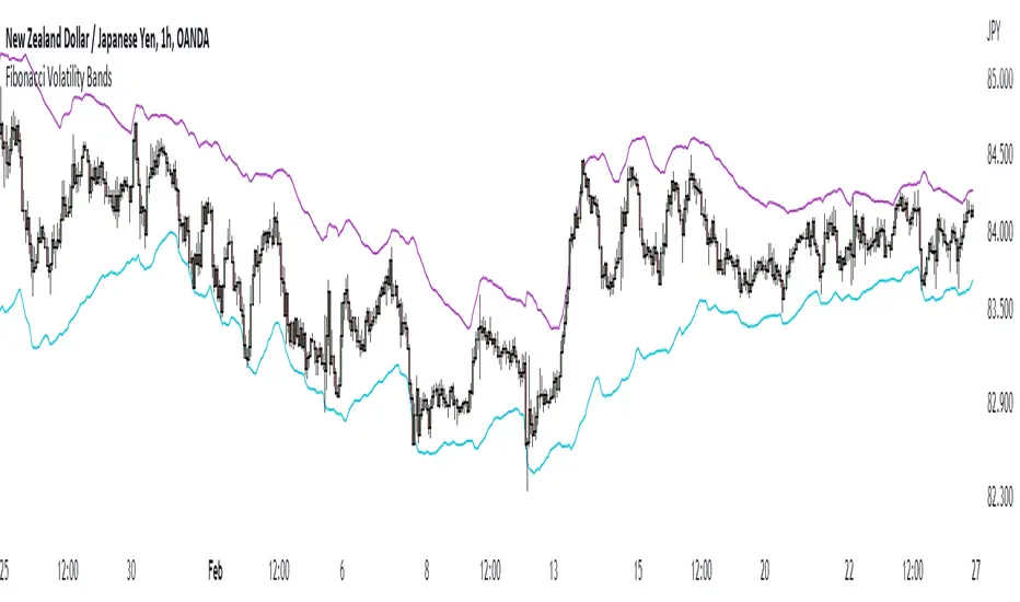
Fibonacci Volatility BandsFibonacci Volatility Bands are just an alternative that allows for more margin than regular Bollinger Bands. They are created based on an average of moving averages that use the Fibonacci sequence as lookback periods.
The use of the Fibonacci Volatility Bands is exactly the same as the Bollinger Bands.
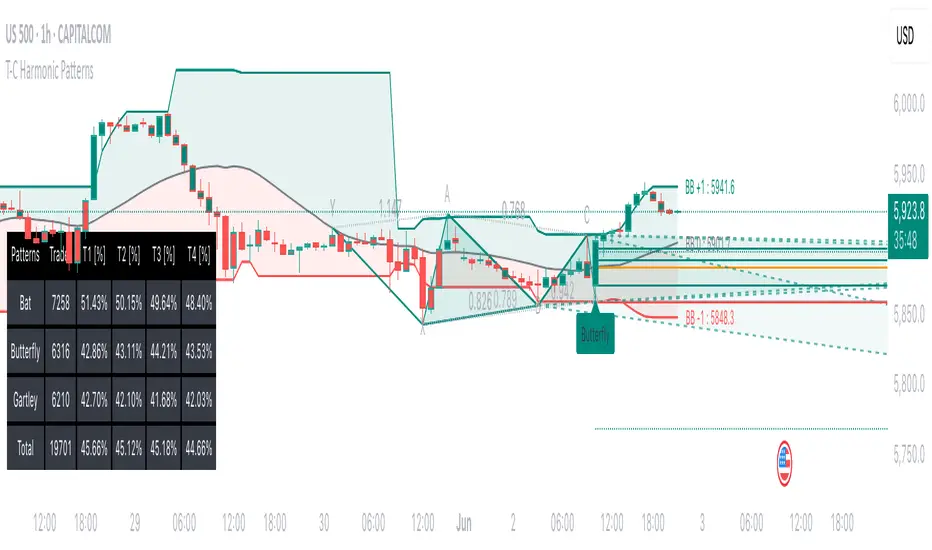
Tailored-Custom Hamonic Patterns█ OVERVIEW
We have included by default 3 known Patterns. The Bat, the Butterfly and the Gartley. But have you ever wondered how effective other,
not yet known models could be? Don't ask yourself the question anymore, it's time to find out for yourself! You have the option to customize
your own Patterns with the Backtesting tool and set Retracement Ratios and Targets for your own Patterns. In addition to this, in order to determine
the Trend at a glance and make Pattern detection more efficient, we have linked the calculation of Patterns to Bands of several types to choose
from (Bollinger, Keltner, Donchian) that you can select from a drop-down menu in the settings and play with the Multiplier
and the Adaptive Length of the Patterns to see how it affects the success rate in the Backtesting table.
█ HOW DOES IT WORK?
- Harmonic Patterns
-Pattern Names, Colors, Style etc… Everything is customizable.
-Dynamic Adaptative Length with Min/Max Length.
- XAB/ABC Ratio
-Min/Max XAB/ABC Configurable Ratio for each Pattern to create your own Patterns.
(This is really the particular option of this Indicator, because it allows you to be able to Backtest in real time
after having played at configuring your own Ratios)
- Bands
-Contrary to the original logic of the HeWhoMustNotBeNamed script, here when the price breaks out of the upper Bands
(example, Bollinger band, Keltner Channel or Donchian Channel) , with a predetermined Minimum and Maximum Length and Multiplier, we can consider
the Trend to be Bearish (and not Bullish) and similarly when the price breaks down in the lower band, we can consider the Trend
to be Bullish (not Bearish) . We have also added the middle line of the Channels (which can be useful for 'Scalper' type Traders.
-The Length of the Bands Filter is directly related to the Dynamic Length of the Patterns.
-You can use a drop-down menu to select from the following Bands Filters :
SMA, EMA, HMA, RMA, WMA, VWMA, HIGH/LOW, LINREG, MEDIAN.
-Sticky and Adaptive Bands options has been included.
- Projections
-BD/CD Projection Ratio configurable for each Pattern.
(Projections are visible as Dotted Lines which we can choose to Extend or not)
- Targets
-Target, PRZ and Stop Levels are set to optimal values based on individual Patterns. (The PRZ Level corresponds to point D
of the detected Pattern so its value should always be 0) but you can change the Targets value (defined in %) as you wish.
Again here, you have the option to fully configure the Style and Extend the Lines or not.
- Backtesting Table
-As said previously, with the possibility of testing the Success Rate of each of the 3 Customizable Patterns,
this option is part of the logic of this Indicator.
- Alerts
-We originally believe that this Indicator does not even need Alerts. But we still decided to include at least one Alert
that you can set for when a new Pattern is detected.
█ NOTES
Thanks to HeWhoMustNotBeNamed for his permission to reuse some part of his zigzag scripts.
Remember to only make a decision once you are sure of your analysis. Good trading sessions to everyone and don't forget,
risk management remains the most important!
Keltner Channels Bands (RMA)Keltner Channel Bands
These normally consist of:
Keltner Channel Upper Band = EMA + Multiplier ∗ ATR
Keltner Channel Lower Band = EMA − Multiplier ∗ ATR
However instead of using ATR we are using RMA
This gives us a much smoother take of the KCB
We are also using 2 sets of bands built on 1 Moving average, this is a common set up for mean reversion strategies.
This can often be paired with RSI for lower timeframe divergences
Divergence
This is using the RSI to calculate when price sets new lows/highs whilst the RSI movement is in the opposite direction.
The way this is calculated is slightly different to traditional divergence scripts. instead of looking for pivot highs/lows in the RSI we are logging the RSI value when price makes it pivot highs/lows.
Gradient Bands
The Gradient Colouring on the bands is measuring how long price has been either side of the MA.
As Keltner bands are commonly used as a mean reversion strategy, I thought it would be useful to see how long price has been trending in a certain direction, the stronger the colours get,
the longer price has been trending that direction which could suggest we are looking for a retrace soon.
Alerts
Alerts included let you choose whether you want to receive an alert for the inside, outside or both band touches.
To set up these alerts, simply toggle them on in the settings, then click on the 3 dots next to the indicators name, from there you click 'Add Alert'.
From there you can customise the alert settings but make sure to leave the 2 top boxes which control the alert conditions. They will be default selected onto your correct settings, the rest you may want to change.
Once you create the alert, it will then trigger as soon as price touches your chosen inside/outside band.
Suggestions
Please feel free to offer any suggestions which you think could improve the script
Disclaimer
The default settings/parameters were shared by Jimtalbott, feel free to play about with the and use this code to make your own strategies.

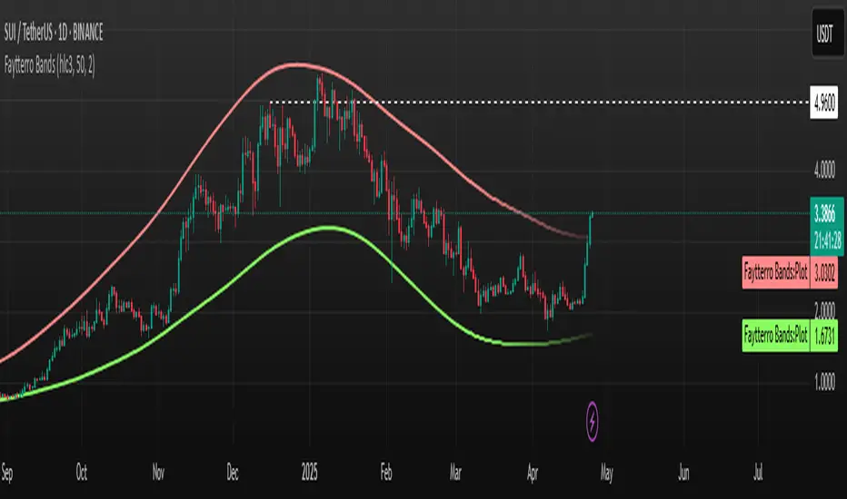
Faytterro Bandswhat is Faytterro Bands?
it is a channel indicator like "Bollinger Bands".
what it does?
creates a channel using standard deviations and means. thus giving users an idea about the expensive and cheap zones. It uses a special weighted moving average different from standard bollinger bands, it also averages not only price but also deviations.
how it does it?
it uses this formulas:
how to use it?
its usage is the same as "bollinger band".
length represents the number of candles to be taken into account, source represents the source of those candles and stdev represents the coefficient of the standard deviation.
you can use it with other indicators:
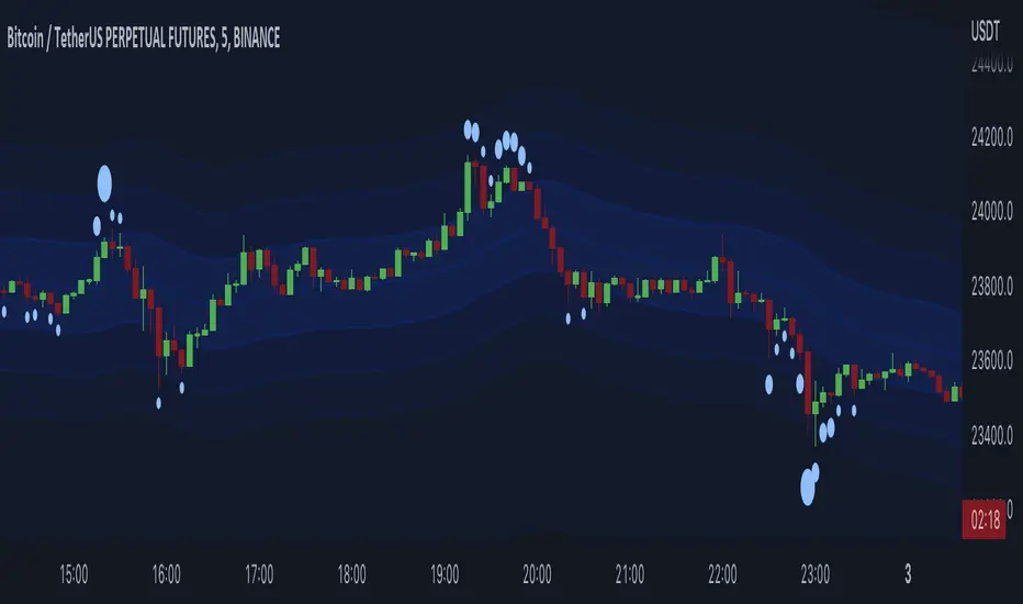
Liquidation Bands (+CVD Bubbles) - By LeviathanAlong with CVD bubbles, this script plots continuous bands that represent 100x, 75x, 50x, 25x liquidation levels. The bands can serve as support/resistance, reversal points, expected volatility range and more.
The indicator uses either the Exponential Moving Average (EMA) or the Volume Weighted Average Price (VWAP) as a base for plotting continuous lines and zones set at the approximate distance of 100x, 75x, 50x, 25x leverage liquidation prices.
These bands can help you visualize:
- Dynamic Support and Resistance levels
- Levels that the price will gravitate towards
- Expected price range (potential volatility)
- Reversal points
- ...
The "CVD Bubbles" part of this script plots circles that are based on my imitation of Cumulative Volume Delta (CVD).
CVD Bubbles will appear when buy/sell volume is increased. The larger the bubble, the more buying/selling at that candle.
"Buy Order" CVD Bubbles appear above candles and might signal:
- Late longers entering the market
- Large short liquidations (closed short=buy order)
- Large market buys getting absorbed by limit sell orders
=> Bias: potential reversal to the downside
"Sell Order" CVD Bubbles appear below candles and might signal:
- Late shorters entering the market
- Large long liquidations (closed long=sell order)
- Large market sells getting absorbed by limit buy orders
=> Bias: potential reversal to the upside
Combining Liquidation Bands and CVD Bubbles can serve you as confluence for taking a trade, but don't follow them blindly.
Settings:
"Mode" - Choose the base for Liquidation Bands (EMA or VWAP)
"EMA/CVD Length" - Choose the length (number of bars) for calculating EMA and CVD
"Level Calculation Mode" - Choose between 3 variations of calculating the distance to Liquidation Bands
"Standard Deviation Length" - Choose the length used for calculating the thresholds of CVD
"Appearance" - Choose the colors of lines, zones and CVD Bubbles
"STDEV MULT." - Multiply the thresholds used for CVD Bubble Sizes
Bollinger Bands [Anan]Hello friends,,
This is my own enhanced version of Bollinger Bands based on some backtesting,,
It's the same logic behind standard BB but instead of using length(period), I created a formula and used a "factor" to scale it up/down.
The formula is just average of averages of averages... (But it's backtested with good results)
I also added two standard deviations so that the distance between them will be the (over-bought/over-sold zones)
And finally added a squeeze indicator to identify the predicted price action movements..
You have the options to control everything like:
-Timeframe
-Source
-Calculation Method
-Length Factor
-StdDev#1
-StdDev#2
-Squeeze Factor
-Squeeze Threshold

LNL Keltner CandlesLNL Keltner Candles
This indicator plots mean reversion (reversal) arrows with custom painted candles based on the price touch or close above or below keltner channel limits (upper & lower bands). This study was created primarily for swing trading & higher time frames such as daily and weekly. Lower time frames might result in more false signals.
Mean Reversal Arrows:
1. Reversal Arrow Up - If the price drops below the lower band extremes, reversal up is the trigger for a bullish mean reversion.
2. Reversal Arrow Down - Once the price reach the higher band extremes, reversal down is the trigger for a bearish mean reversion.
The Concept of Mean Reversion:
There are just two types of moves in any market: The market is either expanding from the mean or retracing back to the mean. These reversions & epxansions are happening across all types of markets. The goal of this study is to catch the powerful mean reversion from extremes back to the mean. Once the candles light up green / red, it is time to look for the reversal (purple) arrow which triggers the mean reversion setup. Mean reversion is not about catching the next big swing turn to new highs or lows. It is all about the base hits = the mean. So the target here is always the average price. The idea here is to catch the average market ebbs & flows, not the next home run.
What Do I Mean by Mean?
Mean is usually the average price from the last 20-30 bars. Basically something like a 20 MA or Keltner Channel or Bollinger Band midline are really good visual representators of the mean (average price).
Hope it helps.
