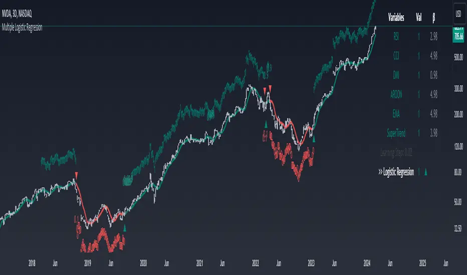
Machine Learning: Multiple Logistic Regression
Multiple Logistic Regression Indicator
The Logistic Regression Indicator for TradingView is a versatile tool that employs multiple logistic regression based on various technical indicators to generate potential buy and sell signals. By utilizing key indicators such as RSI, CCI, DMI, Aroon, EMA, and SuperTrend, the indicator aims to provide a systematic approach to decision-making in financial markets.
How It Works:
Technical Indicators:
The script uses multiple technical indicators such as RSI, CCI, DMI, Aroon, EMA, and SuperTrend as input variables for the logistic regression model.
These indicators are normalized to create categorical variables, providing a consistent scale for the model.
Logistic Regression:
The logistic regression function is applied to the normalized input variables (x1 to x6) with user-defined coefficients (b0 to b6).
The logistic regression model predicts the probability of a binary outcome, with values closer to 1 indicating a bullish signal and values closer to 0 indicating a bearish signal.
Loss Function (Cross-Entropy Loss):
The cross-entropy loss function is calculated to quantify the difference between the predicted probability and the actual outcome.
The goal is to minimize this loss, which essentially measures the model's accuracy.
// Error Function (cross-entropy loss)
loss(y, p) =>
-y * math.log(p) - (1 - y) * math.log(1 - p)
// y - depended variable
// p - multiple logistic regression
Gradient Descent:
Gradient descent is an optimization algorithm used to minimize the loss function by adjusting the weights of the logistic regression model.
The script iteratively updates the weights (b1 to b6) based on the negative gradient of the loss function with respect to each weight.
// Adjusting model weights using gradient descent
b1 -= lr * (p + loss) * x1
b2 -= lr * (p + loss) * x2
b3 -= lr * (p + loss) * x3
b4 -= lr * (p + loss) * x4
b5 -= lr * (p + loss) * x5
b6 -= lr * (p + loss) * x6
// lr - learning rate or step of learning
// p - multiple logistic regression
// x_n - variables
Learning Rate:
The learning rate (lr) determines the step size in the weight adjustment process. It prevents the algorithm from overshooting the minimum of the loss function.
Users can set the learning rate to control the speed and stability of the optimization process.
Visualization:
The script visualizes the output of the logistic regression model by coloring the SMA.
Arrows are plotted at crossover and crossunder points, indicating potential buy and sell signals.
Lables are showing logistic regression values from 1 to 0 above and below bars
Table Display:
A table is displayed on the chart, providing real-time information about the input variables, their values, and the learned coefficients.
This allows traders to monitor the model's interpretation of the technical indicators and observe how the coefficients change over time.
How to Use:
Parameter Adjustment:
Users can adjust the length of technical indicators (rsi_length, cci_length, etc.) and the Z score length based on their preference and market characteristics.
Set the initial values for the regression coefficients (b0 to b6) and the learning rate (lr) according to your trading strategy.
Signal Interpretation:
Buy signals are indicated by an upward arrow (▲), and sell signals are indicated by a downward arrow (▼).
The color-coded SMA provides a visual representation of the logistic regression output by color.
Table Information:
Monitor the table for real-time information on the input variables, their values, and the learned coefficients.
Keep an eye on the learning rate to ensure a balance between model adjustment speed and stability.
Backtesting and Validation:
Before using the script in live trading, conduct thorough backtesting to evaluate its performance under different market conditions.
Validate the model against historical data to ensure its reliability.
Forecast
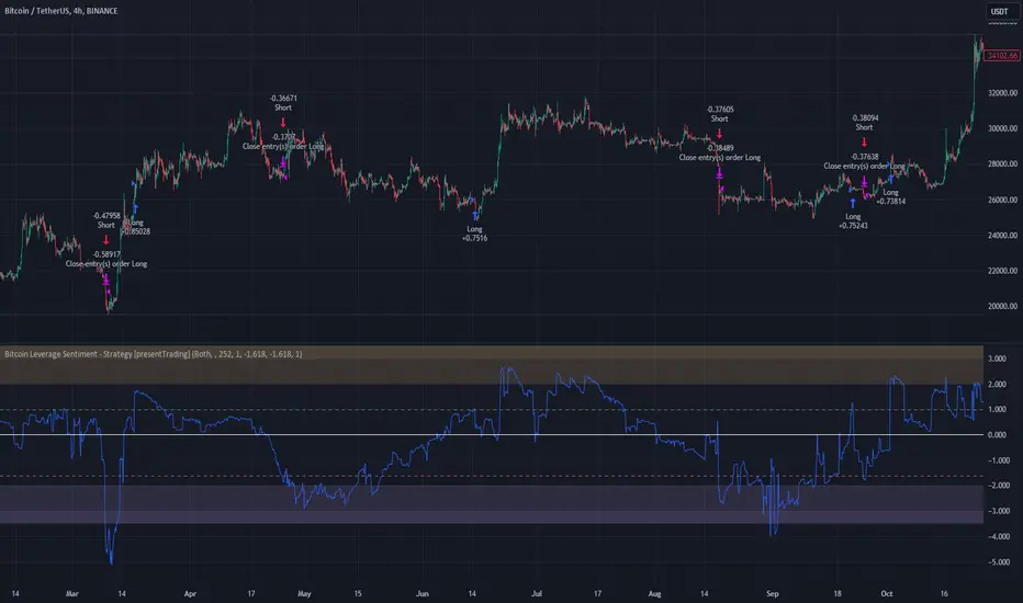
Bitcoin Leverage Sentiment - Strategy [presentTrading]█ Introduction and How it is Different
The "Bitcoin Leverage Sentiment - Strategy " represents a novel approach in the realm of cryptocurrency trading by focusing on sentiment analysis through leveraged positions in Bitcoin. Unlike traditional strategies that primarily rely on price action or technical indicators, this strategy leverages the power of Z-Score analysis to gauge market sentiment by examining the ratio of leveraged long to short positions. By assessing how far the current sentiment deviates from the historical norm, it provides a unique lens to spot potential reversals or continuation in market trends, making it an innovative tool for traders who wish to incorporate market psychology into their trading arsenal.
BTC 4h L/S Performance
local
█ Strategy, How It Works: Detailed Explanation
🔶 Data Collection and Ratio Calculation
Firstly, the strategy acquires data on leveraged long (**`priceLongs`**) and short positions (**`priceShorts`**) for Bitcoin. The primary metric of interest is the ratio of long positions relative to the total of both long and short positions:
BTC Ratio=priceLongs / (priceLongs+priceShorts)
This ratio reflects the prevailing market sentiment, where values closer to 1 indicate a bullish sentiment (dominance of long positions), and values closer to 0 suggest bearish sentiment (prevalence of short positions).
🔶 Z-Score Calculation
The Z-Score is then calculated to standardize the BTC Ratio, allowing for comparison across different time periods. The Z-Score formula is:
Z = (X - μ) / σ
Where:
- X is the current BTC Ratio.
- μ is the mean of the BTC Ratio over a specified period (**`zScoreCalculationPeriod`**).
- σ is the standard deviation of the BTC Ratio over the same period.
The Z-Score helps quantify how far the current sentiment deviates from the historical norm, with high positive values indicating extreme bullish sentiment and high negative values signaling extreme bearish sentiment.
🔶 Signal Generation: Trading signals are derived from the Z-Score as follows:
Long Entry Signal: Occurs when the BTC Ratio Z-Score crosses above the thresholdLongEntry, suggesting bullish sentiment.
- Condition for Long Entry = BTC Ratio Z-Score > thresholdLongEntry
Long Exit/Short Entry Signal: Triggered when the BTC Ratio Z-Score drops below thresholdLongExit for exiting longs or below thresholdShortEntry for entering shorts, indicating a shift to bearish sentiment.
- Condition for Long Exit/Short Entry = BTC Ratio Z-Score < thresholdLongExit or BTC Ratio Z-Score < thresholdShortEntry
Short Exit Signal: Happens when the BTC Ratio Z-Score exceeds the thresholdShortExit, hinting at reducing bearish sentiment and a potential switch to bullish conditions.
- Condition for Short Exit = BTC Ratio Z-Score > thresholdShortExit
🔶Implementation and Visualization: The strategy applies these conditions for trade management, aligning with the selected trade direction. It visualizes the BTC Ratio Z-Score with horizontal lines at entry and exit thresholds, illustrating the current sentiment against historical norms.
█ Trade Direction
The strategy offers flexibility in trade direction, allowing users to choose between long, short, or both, depending on their market outlook and risk tolerance. This adaptability ensures that traders can align the strategy with their individual trading style and market conditions.
█ Usage
To employ this strategy effectively:
1. Customization: Begin by setting the trade direction and adjusting the Z-Score calculation period and entry/exit thresholds to match your trading preferences.
2. Observation: Monitor the Z-Score and its moving average for potential trading signals. Look for crossover events relative to the predefined thresholds to identify entry and exit points.
3. Confirmation: Consider using additional analysis or indicators for signal confirmation, ensuring a comprehensive approach to decision-making.
█ Default Settings
- Trade Direction: Determines if the strategy engages in long, short, or both types of trades, impacting its adaptability to market conditions.
- Timeframe Input: Influences signal frequency and sensitivity, affecting the strategy's responsiveness to market dynamics.
- Z-Score Calculation Period: Affects the strategy’s sensitivity to market changes, with longer periods smoothing data and shorter periods increasing responsiveness.
- Entry and Exit Thresholds: Set the Z-Score levels for initiating or exiting trades, balancing between capturing opportunities and minimizing false signals.
- Impact of Default Settings: Provides a balanced approach to leverage sentiment trading, with adjustments needed to optimize performance across various market conditions.
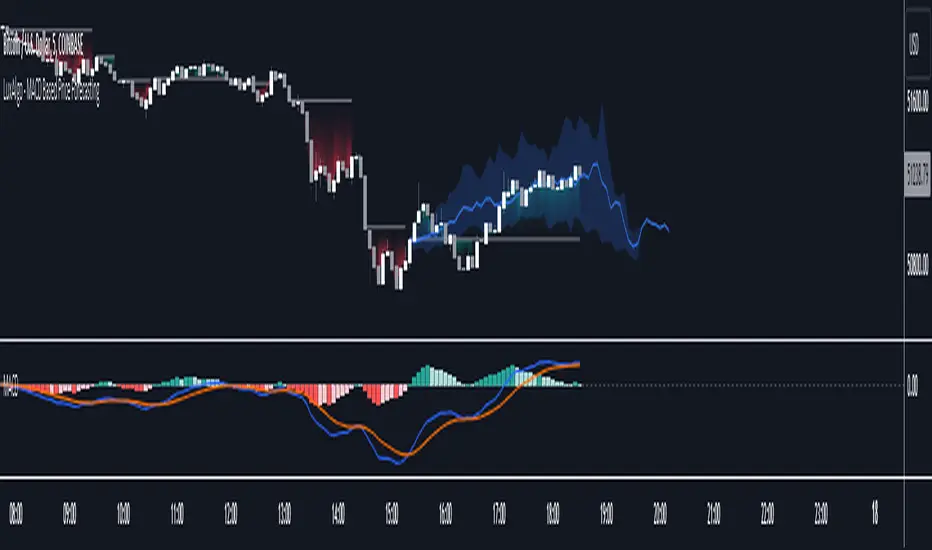
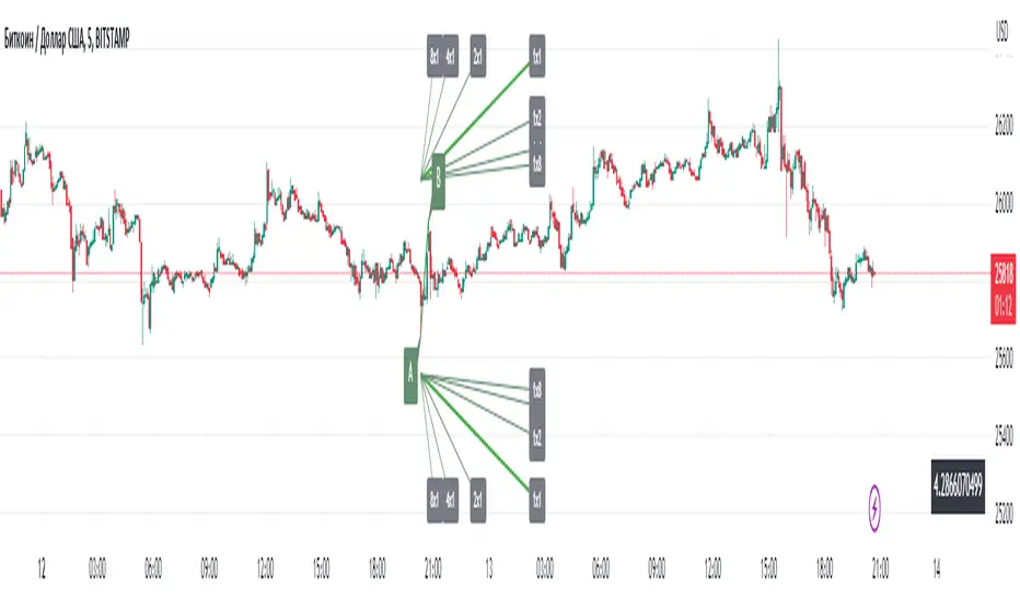
MACD Based Price Forecasting [LuxAlgo]The MACD Based Price Forecasting tool is an innovative price forecasting method based on signals generated by the MACD indicator.
The forecast includes an area which can help traders determine the area where price can develop after a MACD signal.
🔶 USAGE
The forecast returned by the tool allows users to obtain a general picture of how price tends to progress after a specific MACD signal. The forecast is constructed based on percentiles of previous price progressions done after a specific MACD signal is generated.
Users can change which condition is used to generate MACD signals from the "Trend Determination" dropdown menu, with "MACD" determining trends based on whether the MACD is positive (uptrend) or negative (downtrend) and "MACD-Signal" determining trends based on the position of the MACD relative to its signal line, with an MACD above the signal line indicating an uptrend, else a downtrend.
Users can introduce bias to the forecast by changing the "Average Percentage" setting, with values above 50% introducing bullish bias, and below bearish bias.
It can be possible for the forecast to highlight potential reversals depending on the selected forecasting horizon as long as reversals can be observed on trends detected by the MACD.
🔹 Forecasting Area
The forecasting area can help visualize the area that will likely contain price after a specific signal. The area width is based on the "Top/Bottom Percentiles" settings, with a higher "Top Percentile" value returning a higher top bound and a lower "Bottom Percentile" value returning a lower bottom bound.
These areas can also serve as potential support/resistance areas.
🔶 SETTINGS
Fast Length: Fast length of the moving average used to compute the MACD
Slow Length: Slow length of the moving average used to compute the MACD
Signal Length: Length of the MACD moving average.
Trend Determination: Method used to determine a trend direction from the MACD.
🔹 Forecast
Maximum Memory: Determines the maximum amount of prices recorded at each steps succeeding a signal. Lower values will return forecasts with a higher degree of variability.
Forecasting Length: Forecasting horizon in bars, this value only serves as a limit of the forecasting horizon and might not be reached depending on user selected MACD settings.
Top Percentile: Percentile value used to determine the upper bound of the forecasting area.
Average Percentile: Percentile value used to determine the forecast.
Lower Percentile: Percentile value used to determine the lower bound of the forecasting area.
Session breakThis indicator will show future lines before each session start. It will only show London session and US session start.
You can change the color of the lines and time as per day light savings.

AI SuperTrend x Pivot Percentile - Strategy [PresentTrading]█ Introduction and How it is Different
The AI SuperTrend x Pivot Percentile strategy is a sophisticated trading approach that integrates AI-driven analysis with traditional technical indicators. Combining the AI SuperTrend with the Pivot Percentile strategy highlights several key advantages:
1. Enhanced Accuracy in Trend Prediction: The AI SuperTrend utilizes K-Nearest Neighbors (KNN) algorithm for trend prediction, improving accuracy by considering historical data patterns. This is complemented by the Pivot Percentile analysis which provides additional context on trend strength.
2. Comprehensive Market Analysis: The integration offers a multi-faceted approach to market analysis, combining AI insights with traditional technical indicators. This dual approach captures a broader range of market dynamics.
BTC 6H L/S Performance
Local
█ Strategy: How it Works - Detailed Explanation
🔶 AI-Enhanced SuperTrend Indicators
1. SuperTrend Calculation:
- The SuperTrend indicator is calculated using a moving average and the Average True Range (ATR). The basic formula is:
- Upper Band = Moving Average + (Multiplier × ATR)
- Lower Band = Moving Average - (Multiplier × ATR)
- The moving average type (SMA, EMA, WMA, RMA, VWMA) and the length of the moving average and ATR are adjustable parameters.
- The direction of the trend is determined based on the position of the closing price in relation to these bands.
2. AI Integration with K-Nearest Neighbors (KNN):
- The KNN algorithm is applied to predict trend direction. It uses historical price data and SuperTrend values to classify the current trend as bullish or bearish.
- The algorithm calculates the 'distance' between the current data point and historical points. The 'k' nearest data points (neighbors) are identified based on this distance.
- A weighted average of these neighbors' trends (bullish or bearish) is calculated to predict the current trend.
For more please check: Multi-TF AI SuperTrend with ADX - Strategy
🔶 Pivot Percentile Analysis
1. Percentile Calculation:
- This involves calculating the percentile ranks for high and low prices over a set of predefined lengths.
- The percentile function is typically defined as:
- Percentile = Value at (P/100) × (N + 1)th position
- Where P is the desired percentile, and N is the number of data points.
2. Trend Strength Evaluation:
- The calculated percentiles for highs and lows are used to determine the strength of bullish and bearish trends.
- For instance, a high percentile rank in the high prices may indicate a strong bullish trend, and vice versa for bearish trends.
For more please check: Pivot Percentile Trend - Strategy
🔶 Strategy Integration
1. Combining SuperTrend and Pivot Percentile:
- The strategy synthesizes the insights from both AI-enhanced SuperTrend and Pivot Percentile analysis.
- It compares the trend direction indicated by the SuperTrend with the strength of the trend as suggested by the Pivot Percentile analysis.
2. Signal Generation:
- A trading signal is generated when both the AI-enhanced SuperTrend and the Pivot Percentile analysis agree on the trend direction.
- For instance, a bullish signal is generated when both the SuperTrend is bullish, and the Pivot Percentile analysis shows strength in bullish trends.
🔶 Risk Management and Filters
- ADX and DMI Filter: The strategy uses the Average Directional Index (ADX) and the Directional Movement Index (DMI) as filters to assess the trend's strength and direction.
- Dynamic Trailing Stop Loss: Based on the SuperTrend indicator, the strategy dynamically adjusts stop-loss levels to manage risk effectively.
This strategy stands out for its ability to combine real-time AI analysis with established technical indicators, offering traders a nuanced and responsive tool for navigating complex market conditions. The equations and algorithms involved are pivotal in accurately identifying market trends and potential trade opportunities.
█ Usage
To effectively use this strategy, traders should:
1. Understand the AI and Pivot Percentile Indicators: A clear grasp of how these indicators work will enable traders to make informed decisions.
2. Interpret the Signals Accurately: The strategy provides bullish, bearish, and neutral signals. Traders should align these signals with their market analysis and trading goals.
3. Monitor Market Conditions: Given that this strategy is sensitive to market dynamics, continuous monitoring is crucial for timely decision-making.
4. Adjust Settings as Needed: Traders should feel free to tweak the input parameters to suit their trading preferences and to respond to changing market conditions.
█Default Settings and Their Impact on Performance
1. Trading Direction (Default: "Both")
Effect: Determines whether the strategy will take long positions, short positions, or both. Adjusting this setting can align the strategy with the trader's market outlook or risk preference.
2. AI Settings (Neighbors: 3, Data Points: 24)
Neighbors: The number of nearest neighbors in the KNN algorithm. A higher number might smooth out noise but could miss subtle, recent changes. A lower number makes the model more sensitive to recent data but may increase noise.
Data Points: Defines the amount of historical data considered. More data points provide a broader context but may dilute recent trends' impact.
3. SuperTrend Settings (Length: 10, Factor: 3.0, MA Source: "WMA")
Length: Affects the sensitivity of the SuperTrend indicator. A longer length results in a smoother, less sensitive indicator, ideal for long-term trends.
Factor: Determines the bandwidth of the SuperTrend. A higher factor creates wider bands, capturing larger price movements but potentially missing short-term signals.
MA Source: The type of moving average used (e.g., WMA - Weighted Moving Average). Different MA types can affect the trend indicator's responsiveness and smoothness.
4. AI Trend Prediction Settings (Price Trend: 10, Prediction Trend: 80)
Price Trend and Prediction Trend Lengths: These settings define the lengths of weighted moving averages for price and SuperTrend, impacting the responsiveness and smoothness of the AI's trend predictions.
5. Pivot Percentile Settings (Length: 10)
Length: Influences the calculation of pivot percentiles. A shorter length makes the percentile more responsive to recent price changes, while a longer length offers a broader view of price trends.
6. ADX and DMI Settings (ADX Length: 14, Time Frame: 'D')
ADX Length: Defines the period for the Average Directional Index calculation. A longer period results in a smoother ADX line.
Time Frame: Sets the time frame for the ADX and DMI calculations, affecting the sensitivity to market changes.
7. Commission, Slippage, and Initial Capital
These settings relate to transaction costs and initial investment, directly impacting net profitability and strategy feasibility.

ATH Gain PotentialThe indicator quantifies the relative position of a symbol's current closing price in relation to its historical all-time high (ATH).
By evaluating the ratio between the ATH and the present closing price, it provides an analytical framework to estimate the potential gains that could accrue if the symbol were to revert to its ATH from a specified reference point. The ratio serves as a quantitative measure for assessing the distance between the current market value and the symbol's historical peak, enabling investors to gauge the prospective profitability of a return to the ATH.

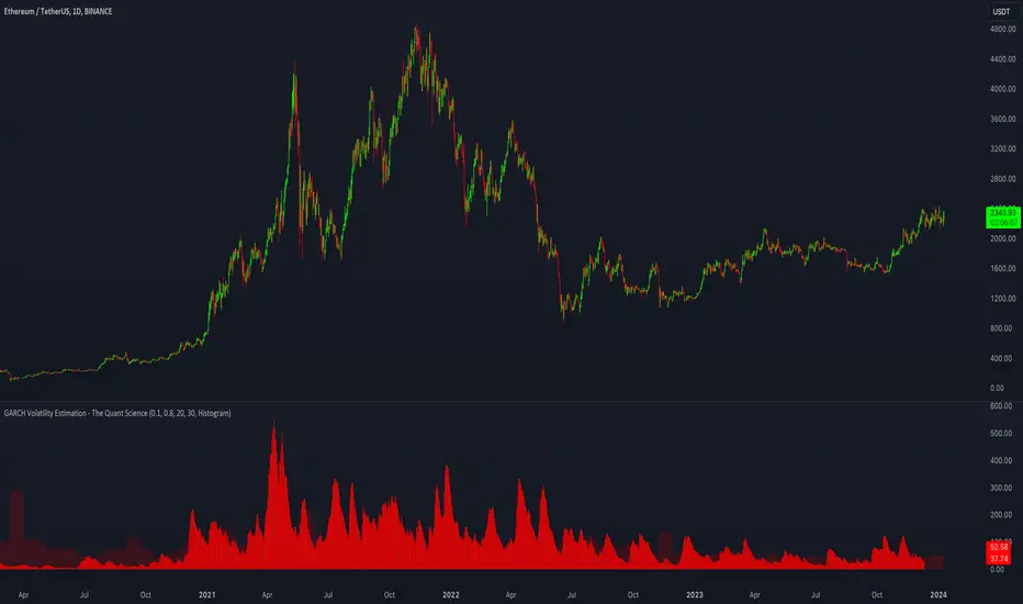
GARCH Volatility Estimation - The Quant ScienceThe GARCH (Generalized Autoregressive Conditional Heteroskedasticity) model is a statistical model used to forecast the volatility of a financial asset. This model takes into account the fluctuations in volatility over time, recognizing that volatility can vary in a heteroskedastic (i.e., non-constant variance) manner and can be influenced by past events.
The general formula of the GARCH model is:
σ²(t) = ω + α * ε²(t-1) + β * σ²(t-1)
where:
σ²(t) is the conditional variance at time t (i.e., squared volatility)
ω is the constant term (intercept) representing the baseline level of volatility
α is the coefficient representing the impact of the squared lagged error term on the conditional variance
ε²(t-1) is the squared lagged error term at the previous time period
β is the coefficient representing the impact of the lagged conditional variance on the current conditional variance
In the context of financial forecasting, the GARCH model is used to estimate the future volatility of the asset.
HOW TO USE
This quantitative indicator is capable of estimating the probable future movements of volatility. When the GARCH increases in value, it means that the volatility of the asset will likely increase as well, and vice versa. The indicator displays the relationship of the GARCH (bright red) with the trend of historical volatility (dark red).
USER INTERFACE
Alpha: select the starting value of Alpha (default value is 0.10).
Beta: select the starting value of Beta (default value is 0.80).
Lenght: select the period for calculating values within the model such as EMA (Exponential Moving Average) and Historical Volatility (default set to 20).
Forecasting: select the forecasting period, the number of bars you want to visualize data ahead (default set to 30).
Design: customize the indicator with your preferred color and choose from different types of charts, managing the design settings.
Forecast: PastFluxDelta PredictionThe theory is that time periods and the conditions during these periods repeat themselves. Especially if it is the same day of the week in the past, there is a high probability that price fluctuations will roughly repeat themselves.
Eternal return (or eternal recurrence) is a philosophical concept which states that time repeats itself in an infinite loop, and that exactly the same events will continue to occur in exactly the same way, over and over again, for eternity.
History does repeat itself.
The stock market is a manifest example.
Chief market strategist at Miller Tabak + Co. Matt Maley pointed out the strong resemblance between the stock market recently and that in the past.
Various scientific studies and articles show that there could be something to this theory
Most of the investors are ignoring the parallels between stocks today and "heady" years 1929, 1999 and 2007…
Post Labor Day sees investors returning to the S&P 500 near all-time highs and some dark economic shadows lurking …
So how should we regard these inescapable results?
Nietzsche said we should embrace them, accept them, and love them. Once they stop, expect them to start again.
But remember that the future is fundamentally uncertain and that past results are by no means a guarantee of future performance.
Based on this, this indicator uses historical trading data from a year, a week or a day ago and compares price fluctuations in the past with current conditions.
"Bars to predict" can be used to indicate how far into the future the indicator is looking.
"Amount of bars to show" determines how many bars are generally displayed. A high value allows you to see how accurate the method was in the past.

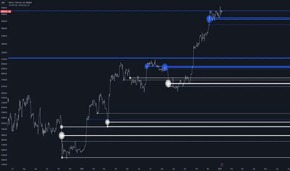
Whalemap [BigBeluga]The Whalemap indicator aims to spot big buying and selling activity represented as big orders for a possible bottom or top formation on the chart.
🔶 CALCULATION
The indicator uses volume to spot big volume activity represented as big orders in the market.
for i = 0 to len - 1
blV.vol += (close > close ? volume : 0)
brV.vol += (close < close ? volume : 0)
When volume exceeds its own threshold, it is a sign that volume is exceeding its normal value and is considered as a "Whale order" or "Whale activity," which is then plotted on the chart as circles.
🔶 DETAILS
The indicator plots Bubbles on the chart with different sizes indicating the buying or selling activity. The bigger the circle, the more impact it will have on the market.
On each circle is also plotted a line, and its own weight is also determined by the strength of its own circle; the bigger the circle, the bigger the line.
Old buying/selling activity can also be used for future support and resistance to spot interesting areas.
The more price enters old buying/selling activity and starts producing orders of the same direction, it might be an interesting point to take a closer look.
🔶 EXAMPLES
The chart above is showing us price reacting to big orders, finding good bottoms in price and good tops in confluence with old activity.
🔶 SETTINGS
Users will have the options to:
Filter options to adjust buying and selling sensitivity.
Display/Hide Lines
Display/Hide Bubbles
Choose which orders to display (from smallest to biggest)
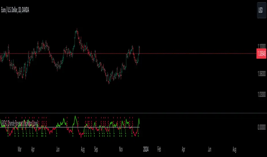
GKD-C Chande Forecast Oscillator [Loxx]The Giga Kaleidoscope GKD-C Chande Forecast Oscillator is a confirmation module included in Loxx's "Giga Kaleidoscope Modularized Trading System."
█ GKD-C Chande Forecast Oscillator
The Chande Forecast Oscillator (CFO) is a technical analysis tool developed by Tushar Chande. It operates by plotting the percentage difference between the closing price and a linear regression forecasted price over a specified number of periods, often referred to as 'n-periods' or 'x-periods'. The essence of this oscillator is to compare actual prices with forecasted ones, thereby providing insights into the momentum and potential trend direction of a financial instrument.
The calculation involves taking the current closing price, subtracting it from the n-period simple moving average, and then dividing this number by the total of the absolute differences between the closing price and the moving average over the same period. The CFO value is positive (above zero) when the forecast price is greater than the closing price, indicating a potential upward trend. Conversely, it is negative (below zero) when the forecast price is less than the closing price, suggesting a downward trend.
█ Giga Kaleidoscope Modularized Trading System
Core components of an NNFX algorithmic trading strategy
The NNFX algorithm is built on the principles of trend, momentum, and volatility. There are six core components in the NNFX trading algorithm:
1. Volatility - price volatility; e.g., Average True Range, True Range Double, Close-to-Close, etc.
2. Baseline - a moving average to identify price trend
3. Confirmation 1 - a technical indicator used to identify trends
4. Confirmation 2 - a technical indicator used to identify trends
5. Continuation - a technical indicator used to identify trends
6. Volatility/Volume - a technical indicator used to identify volatility/volume breakouts/breakdown
7. Exit - a technical indicator used to determine when a trend is exhausted
8. Metamorphosis - a technical indicator that produces a compound signal from the combination of other GKD indicators*
*(not part of the NNFX algorithm)
What is Volatility in the NNFX trading system?
In the NNFX (No Nonsense Forex) trading system, ATR (Average True Range) is typically used to measure the volatility of an asset. It is used as a part of the system to help determine the appropriate stop loss and take profit levels for a trade. ATR is calculated by taking the average of the true range values over a specified period.
True range is calculated as the maximum of the following values:
-Current high minus the current low
-Absolute value of the current high minus the previous close
-Absolute value of the current low minus the previous close
ATR is a dynamic indicator that changes with changes in volatility. As volatility increases, the value of ATR increases, and as volatility decreases, the value of ATR decreases. By using ATR in NNFX system, traders can adjust their stop loss and take profit levels according to the volatility of the asset being traded. This helps to ensure that the trade is given enough room to move, while also minimizing potential losses.
Other types of volatility include True Range Double (TRD), Close-to-Close, and Garman-Klass
What is a Baseline indicator?
The baseline is essentially a moving average, and is used to determine the overall direction of the market.
The baseline in the NNFX system is used to filter out trades that are not in line with the long-term trend of the market. The baseline is plotted on the chart along with other indicators, such as the Moving Average (MA), the Relative Strength Index (RSI), and the Average True Range (ATR).
Trades are only taken when the price is in the same direction as the baseline. For example, if the baseline is sloping upwards, only long trades are taken, and if the baseline is sloping downwards, only short trades are taken. This approach helps to ensure that trades are in line with the overall trend of the market, and reduces the risk of entering trades that are likely to fail.
By using a baseline in the NNFX system, traders can have a clear reference point for determining the overall trend of the market, and can make more informed trading decisions. The baseline helps to filter out noise and false signals, and ensures that trades are taken in the direction of the long-term trend.
What is a Confirmation indicator?
Confirmation indicators are technical indicators that are used to confirm the signals generated by primary indicators. Primary indicators are the core indicators used in the NNFX system, such as the Average True Range (ATR), the Moving Average (MA), and the Relative Strength Index (RSI).
The purpose of the confirmation indicators is to reduce false signals and improve the accuracy of the trading system. They are designed to confirm the signals generated by the primary indicators by providing additional information about the strength and direction of the trend.
Some examples of confirmation indicators that may be used in the NNFX system include the Bollinger Bands, the MACD (Moving Average Convergence Divergence), and the MACD Oscillator. These indicators can provide information about the volatility, momentum, and trend strength of the market, and can be used to confirm the signals generated by the primary indicators.
In the NNFX system, confirmation indicators are used in combination with primary indicators and other filters to create a trading system that is robust and reliable. By using multiple indicators to confirm trading signals, the system aims to reduce the risk of false signals and improve the overall profitability of the trades.
What is a Continuation indicator?
In the NNFX (No Nonsense Forex) trading system, a continuation indicator is a technical indicator that is used to confirm a current trend and predict that the trend is likely to continue in the same direction. A continuation indicator is typically used in conjunction with other indicators in the system, such as a baseline indicator, to provide a comprehensive trading strategy.
What is a Volatility/Volume indicator?
Volume indicators, such as the On Balance Volume (OBV), the Chaikin Money Flow (CMF), or the Volume Price Trend (VPT), are used to measure the amount of buying and selling activity in a market. They are based on the trading volume of the market, and can provide information about the strength of the trend. In the NNFX system, volume indicators are used to confirm trading signals generated by the Moving Average and the Relative Strength Index. Volatility indicators include Average Direction Index, Waddah Attar, and Volatility Ratio. In the NNFX trading system, volatility is a proxy for volume and vice versa.
By using volume indicators as confirmation tools, the NNFX trading system aims to reduce the risk of false signals and improve the overall profitability of trades. These indicators can provide additional information about the market that is not captured by the primary indicators, and can help traders to make more informed trading decisions. In addition, volume indicators can be used to identify potential changes in market trends and to confirm the strength of price movements.
What is an Exit indicator?
The exit indicator is used in conjunction with other indicators in the system, such as the Moving Average (MA), the Relative Strength Index (RSI), and the Average True Range (ATR), to provide a comprehensive trading strategy.
The exit indicator in the NNFX system can be any technical indicator that is deemed effective at identifying optimal exit points. Examples of exit indicators that are commonly used include the Parabolic SAR, the Average Directional Index (ADX), and the Chande Forecast Oscillator.
The purpose of the exit indicator is to identify when a trend is likely to reverse or when the market conditions have changed, signaling the need to exit a trade. By using an exit indicator, traders can manage their risk and prevent significant losses.
In the NNFX system, the exit indicator is used in conjunction with a stop loss and a take profit order to maximize profits and minimize losses. The stop loss order is used to limit the amount of loss that can be incurred if the trade goes against the trader, while the take profit order is used to lock in profits when the trade is moving in the trader's favor.
Overall, the use of an exit indicator in the NNFX trading system is an important component of a comprehensive trading strategy. It allows traders to manage their risk effectively and improve the profitability of their trades by exiting at the right time.
What is an Metamorphosis indicator?
The concept of a metamorphosis indicator involves the integration of two or more GKD indicators to generate a compound signal. This is achieved by evaluating the accuracy of each indicator and selecting the signal from the indicator with the highest accuracy. As an illustration, let's consider a scenario where we calculate the accuracy of 10 indicators and choose the signal from the indicator that demonstrates the highest accuracy.
The resulting output from the metamorphosis indicator can then be utilized in a GKD-BT backtest by occupying a slot that aligns with the purpose of the metamorphosis indicator. The slot can be a GKD-B, GKD-C, or GKD-E slot, depending on the specific requirements and objectives of the indicator. This allows for seamless integration and utilization of the compound signal within the GKD-BT framework.
How does Loxx's GKD (Giga Kaleidoscope Modularized Trading System) implement the NNFX algorithm outlined above?
Loxx's GKD v2.0 system has five types of modules (indicators/strategies). These modules are:
1. GKD-BT - Backtesting module (Volatility, Number 1 in the NNFX algorithm)
2. GKD-B - Baseline module (Baseline and Volatility/Volume, Numbers 1 and 2 in the NNFX algorithm)
3. GKD-C - Confirmation 1/2 and Continuation module (Confirmation 1/2 and Continuation, Numbers 3, 4, and 5 in the NNFX algorithm)
4. GKD-V - Volatility/Volume module (Confirmation 1/2, Number 6 in the NNFX algorithm)
5. GKD-E - Exit module (Exit, Number 7 in the NNFX algorithm)
6. GKD-M - Metamorphosis module (Metamorphosis, Number 8 in the NNFX algorithm, but not part of the NNFX algorithm)
(additional module types will added in future releases)
Each module interacts with every module by passing data to A backtest module wherein the various components of the GKD system are combined to create a trading signal.
That is, the Baseline indicator passes its data to Volatility/Volume. The Volatility/Volume indicator passes its values to the Confirmation 1 indicator. The Confirmation 1 indicator passes its values to the Confirmation 2 indicator. The Confirmation 2 indicator passes its values to the Continuation indicator. The Continuation indicator passes its values to the Exit indicator, and finally, the Exit indicator passes its values to the Backtest strategy.
This chaining of indicators requires that each module conform to Loxx's GKD protocol, therefore allowing for the testing of every possible combination of technical indicators that make up the six components of the NNFX algorithm.
What does the application of the GKD trading system look like?
Example trading system:
Backtest: Multi-Ticker CC Backtest
Baseline: Hull Moving Average
Volatility/Volume: Hurst Exponent
Confirmation 1: Advance Trend Pressure as shown on the chart above
Confirmation 2: uf2018
Continuation: Coppock Curve
Exit: Rex Oscillator
Metamorphosis: Baseline Optimizer
Each GKD indicator is denoted with a module identifier of either: GKD-BT, GKD-B, GKD-C, GKD-V, GKD-M, or GKD-E. This allows traders to understand to which module each indicator belongs and where each indicator fits into the GKD system.
? Giga Kaleidoscope Modularized Trading System Signals
Standard Entry
1. GKD-C Confirmation gives signal
2. Baseline agrees
3. Price inside Goldie Locks Zone Minimum
4. Price inside Goldie Locks Zone Maximum
5. Confirmation 2 agrees
6. Volatility/Volume agrees
1-Candle Standard Entry
1a. GKD-C Confirmation gives signal
2a. Baseline agrees
3a. Price inside Goldie Locks Zone Minimum
4a. Price inside Goldie Locks Zone Maximum
Next Candle
1b. Price retraced
2b. Baseline agrees
3b. Confirmation 1 agrees
4b. Confirmation 2 agrees
5b. Volatility/Volume agrees
Baseline Entry
1. GKD-B Baseline gives signal
2. Confirmation 1 agrees
3. Price inside Goldie Locks Zone Minimum
4. Price inside Goldie Locks Zone Maximum
5. Confirmation 2 agrees
6. Volatility/Volume agrees
7. Confirmation 1 signal was less than 'Maximum Allowable PSBC Bars Back' prior
1-Candle Baseline Entry
1a. GKD-B Baseline gives signal
2a. Confirmation 1 agrees
3a. Price inside Goldie Locks Zone Minimum
4a. Price inside Goldie Locks Zone Maximum
5a. Confirmation 1 signal was less than 'Maximum Allowable PSBC Bars Back' prior
Next Candle
1b. Price retraced
2b. Baseline agrees
3b. Confirmation 1 agrees
4b. Confirmation 2 agrees
5b. Volatility/Volume agrees
Volatility/Volume Entry
1. GKD-V Volatility/Volume gives signal
2. Confirmation 1 agrees
3. Price inside Goldie Locks Zone Minimum
4. Price inside Goldie Locks Zone Maximum
5. Confirmation 2 agrees
6. Baseline agrees
7. Confirmation 1 signal was less than 7 candles prior
1-Candle Volatility/Volume Entry
1a. GKD-V Volatility/Volume gives signal
2a. Confirmation 1 agrees
3a. Price inside Goldie Locks Zone Minimum
4a. Price inside Goldie Locks Zone Maximum
5a. Confirmation 1 signal was less than 'Maximum Allowable PSVVC Bars Back' prior
Next Candle
1b. Price retraced
2b. Volatility/Volume agrees
3b. Confirmation 1 agrees
4b. Confirmation 2 agrees
5b. Baseline agrees
Confirmation 2 Entry
1. GKD-C Confirmation 2 gives signal
2. Confirmation 1 agrees
3. Price inside Goldie Locks Zone Minimum
4. Price inside Goldie Locks Zone Maximum
5. Volatility/Volume agrees
6. Baseline agrees
7. Confirmation 1 signal was less than 7 candles prior
1-Candle Confirmation 2 Entry
1a. GKD-C Confirmation 2 gives signal
2a. Confirmation 1 agrees
3a. Price inside Goldie Locks Zone Minimum
4a. Price inside Goldie Locks Zone Maximum
5a. Confirmation 1 signal was less than 'Maximum Allowable PSC2C Bars Back' prior
Next Candle
1b. Price retraced
2b. Confirmation 2 agrees
3b. Confirmation 1 agrees
4b. Volatility/Volume agrees
5b. Baseline agrees
PullBack Entry
1a. GKD-B Baseline gives signal
2a. Confirmation 1 agrees
3a. Price is beyond 1.0x Volatility of Baseline
Next Candle
1b. Price inside Goldie Locks Zone Minimum
2b. Price inside Goldie Locks Zone Maximum
3b. Confirmation 1 agrees
4b. Confirmation 2 agrees
5b. Volatility/Volume agrees
Continuation Entry
1. Standard Entry, 1-Candle Standard Entry, Baseline Entry, 1-Candle Baseline Entry, Volatility/Volume Entry, 1-Candle Volatility/Volume Entry, Confirmation 2 Entry, 1-Candle Confirmation 2 Entry, or Pullback entry triggered previously
2. Baseline hasn't crossed since entry signal trigger
4. Confirmation 1 agrees
5. Baseline agrees
6. Confirmation 2 agrees
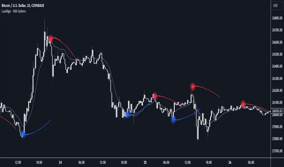
MA Sabres [LuxAlgo]The "MA Sabres" indicator highlights potential trend reversals based on a moving average direction. Detected reversals are accompanied by an extrapolated "Sabre" looking shape that can be used as support/resistance and as a source of breakouts.
🔶 USAGE
If a selected moving average (MA) continues in the same direction for a certain time, a change in that direction could signify a potential reversal.
In this publication, when a trend change occurs, a sabre-shaped figure is drawn which can be used as support/resistance:
A sabre can be indicative of a direction, however, it can also act as a stop-loss when the price should go in the opposite direction:
Or show potential areas of interest:
🔶 DETAILS
This publication will look for a change in direction after the MA went in the same direction during x consecutive bars (settings: " Reversal after x bars in the same direction ").
Then a circle-shaped drawing will be drawn 1 bar back, at the previous high/low, dependable of the previous direction.
From there originates a sabre-shaped figure where the tip lies as far as the user-set MA length.
The angle of the "sabre" relies on the ATR of the previous 14 bars.
Less volatility will create a flatter sabre while the opposite is true when there is more volatility in the previous 14 bars.
The sabre is created by the latest feature, polylines , which enables us to connect several 'points', resulting in a polyline.new() object.
Do note that sabres are offset by one bar to the past to align their locations.
🔶 SETTINGS
MA Type: SMA, EMA, SMMA (RMA), HullMA, WMA, VWMA, DEMA, TEMA, NONE (off)
Length: this sets the length of MA, and the length of the sabre shape
Previous Trend Duration: After the MA direction is the same for x consecutive bars, the first time the direction changes, a sabre is drawn
Machine Learning: Gaussian Process Regression [LuxAlgo]We provide an implementation of the Gaussian Process Regression (GPR), a popular machine-learning method capable of estimating underlying trends in prices as well as forecasting them.
While this implementation is adapted to real-time usage, do remember that forecasting trends in the market is challenging, do not use this tool as a standalone for your trading decisions.
🔶 USAGE
The main goal of our implementation of GPR is to forecast trends. The method is applied to a subset of the most recent prices, with the Training Window determining the size of this subset.
Two user settings controlling the trend estimate are available, Smooth and Sigma . Smooth determines the smoothness of our estimate, with higher values returning smoother results suitable for longer-term trend estimates.
Sigma controls the amplitude of the forecast, with values closer to 0 returning results with a higher amplitude. Do note that due to the calculation of the method, lower values of sigma can return errors with higher values of the training window.
🔹 Updating Mechanisms
The script includes three methods to update a forecast. By default a forecast will not update for new bars (Lock Forecast).
The forecast can be re-estimated once the price reaches the end of the forecasting window when using the "Update Once Reached" method.
Finally "Continuously Update" will update the whole forecast on any new bar.
🔹 Estimating Trends
Gaussian Process Regression can be used to estimate past underlying local trends in the price, allowing for a noise-free interpretation of trends.
This can be useful for performing descriptive analysis, such as highlighting patterns more easily.
🔶 SETTINGS
Training Window: Number of most recent price observations used to fit the model
Forecasting Length: Forecasting horizon, determines how many bars in the future are forecasted.
Smooth: Controls the degree of smoothness of the model fit.
Sigma: Noise variance. Controls the amplitude of the forecast, lower values will make it more sensitive to outliers.
Update: Determines when the forecast is updated, by default the forecast is not updated for new bars.

Rug Pull DetectorOverview
Have you ever wondered why tickers have such erratic movements that seemingly come from nowhere? These "rug pull" events happen quite often and can catch even the most seasoned traders off-guard.
Unlike most other indicators which rely on historical data to make inferences about future price movements, the Rug Pull Detector (RPD) enables you to take a glimpse into market makers' delta-neutral hedging in real-time.
Market makers by nature must be delta-neutral which means that they cannot position themselves to profit from providing liquidity (either long or short). Liquidity provided to the short or long side must end up in a stock purchase or sale to neutralize the trade.
Volatile movements in a ticker's price movement most often result directly after a period of extremely low volatility. These volatile movements are very often "rug pulled" which ends up reverting the ticker back to the price at which the event first occurred. RPD shows these events in real-time. This knowledge can be used to help determine the most probable near-future direction a ticker will gravitate towards after a rug pull event occurs.
Usage
RPD works on any ticker and on any timeframe and can be used as a tool in determining an exit price for a trade. Vertical shading on the chart indicates a warning signal that a rug pull event may be about to kick-off. Once a rug pull event has occurred and is confirmed, a blue label will appear on the chart with a price. A line is then drawn from the bar at which the event occurred and is extended to each subsequent bar until the price is reached once more; thus concluding the event. Furthermore, red or green shading will be present to easily visually identify rug pull events on the chart and whether they are risks to the downside (red) or upside (green). RPD is broken down into 2 main types of events:
Active Event - These events are characterized by a red or green shading and a blue price line.
Dormant Event - These events do not have shading but are still identifiable via a blue price line. Active events that are superseded by newer events will become dormant.
Active events tend to have a higher chance to return to the initial price point and tend to arrive there quicker.
Dormant events have a slightly lower chance to return to the initial price point and may take longer to arrive there.
Please note:
This indicator has no way of telling the exact amount of time that will pass before the ticker returns to the identified price; however, in more cases than not - the ticker will return to that price within a reasonable amount of time relative to the timeframe you are viewing.
There is a small chance any single event will never conclude. These are anomalies and do occur on occasion.
Using RPD alongside tools such as the RSI, Anchored VWAP, or other trend-based indicators will help determine when the ticker's price might be about to pivot and head back towards the identified price point.
Seeing is Believing:
SPY 1D downside rug-pull
----------------------------------------------
AAPL 15s downside and upside rug-pulls
----------------------------------------------
AMD 2D downside rug-pull
----------------------------------------------
VIX 1h downside and upside rug-pulls
Want to see more? Check out my recent Ideas for more examples of the Rug Pull Detector in action.
Disclaimer:
Any information in relation to the Rug Pull Detector does not constitute any financial, investment, or trading advice. Trade or invest at your own risk.

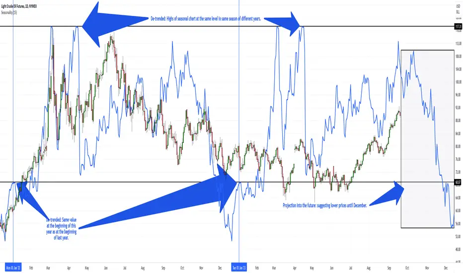
Kaschko's Seasonal TrendThis script calculates the average price moves (using each bar's close minus the previous bar's close) for the trading days, weeks or months (depending on the timeframe it is applied to) of a number of past calendar years (up to 30) to construct a seasonal trend which is then drawn as a seasonal chart (overlay) onto the price chart. Supported are the 1D,1W,1M timeframes.
The seasonal chart is adjusted to the price chart (so that both occupy the same height on the overall chart) and it is also de-trended, which means that the seasonal chart's starting value is the same in each year and the progression during the year is adjusted so that no abrupt gap occurs between years and the highs and lows of consecutive years of the seasonal chart (if projected over more than one year) are also at the same level. Of course, this also means that the absolute value of the seasonal chart has no meaning at all.
You can configure the number of bars the seasonal chart is drawn into the future. This projection shows how price could move in the future if the market shows the same seasonal tendencies like in the past. On the daily chart, the trading week of year (TWOY), trading day of month (TDOM) and trading day of year (TDOY) are shown in the status line.
Caution is advised as seasonality is based on the past. It is not a reliable prediction of the future. But it can still be used as an additional confirmation or contradiction of an otherwise recognized possible impending trend.
I have used a virtually identical indicator for a long time in a commercial software package popular among futures traders, but have not found anything comparable here. Therefore I implemented it myself. I hope you find it useful.
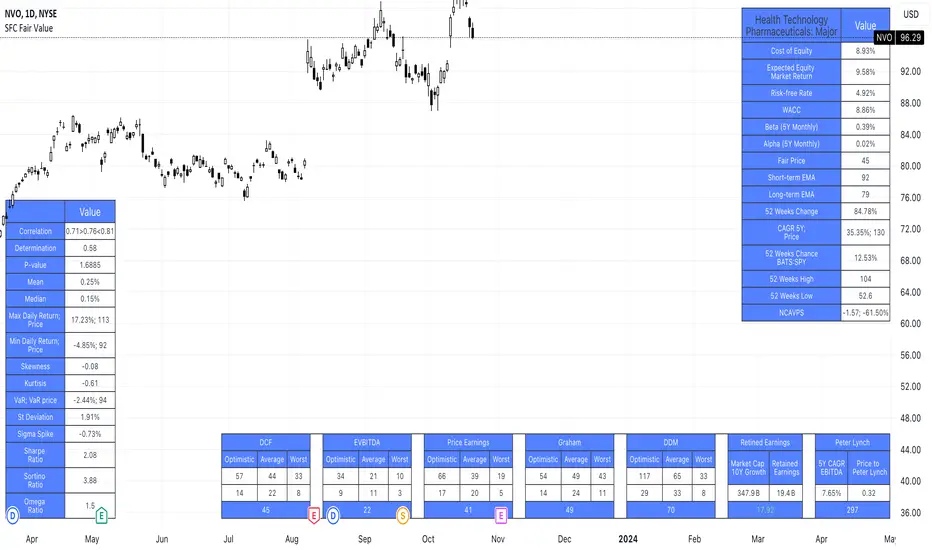
SFC Valuation Model - Fair ValueValuation is the analytical process of determining the current (or projected) worth of an asset or a company. There are many techniques used for doing a valuation. An analyst placing a value on a company looks at the business's management, the composition of its capital structure, the prospect of future earnings, and the market value of its assets, among other metrics.
Fundamental analysis is often employed in valuation, although several other methods may be employed such as the capital asset pricing model (CAPM) or the dividend discount model (DDM), Discounted Cash Flow (DCF) and many others.
A valuation can be useful when trying to determine the fair value of a security, which is determined by what a buyer is willing to pay a seller, assuming both parties enter the transaction willingly. When a security trades on an exchange, buyers and sellers determine the market value of a stock or bond.
There is no universal standard for calculating the intrinsic value of a company or stock. Financial analysts attempt to determine an asset's intrinsic value by using fundamental and technical analyses to gauge its actual financial performance.
Intrinsic value is useful because it can help an investor understand whether a potential investment is overvalued or undervalued.
This indicator allows investors to simulate different scenarios depending on their view of the stock's value. It calculates different models automatically, but users can define the fair value manually by changing the settings.
For example: change the weight of the model; choose how conservatively want to evaluate the stock; use different growth rate or discount rate and so on.
The indicator shows other useful metrics in order to help investors to evaluate the stock.
This indicator can save users hours of searching financial data and calculating fair value.
There are few valuation methods/steps
- Macroeconomics - analyse the current economic;
- Define how the sector is performing;
- Relative valuation method - compare few stocks and find the Outlier;
- Absolute valuation method historically- define how the stock performed in the past;
- Absolute valuation method - define how the stock is performed now and find the fair value;
- Technical analysis
How to use:
1. Once you have completed the initial evaluation steps, simply load the indicator.
2. Check the default settings and see if they suit you.
3. Find the fair value and wait for the stock to reach it.
Machine Learning Regression Trend [LuxAlgo]The Machine Learning Regression Trend tool uses random sample consensus (RANSAC) to fit and extrapolate a linear model by discarding potential outliers, resulting in a more robust fit.
🔶 USAGE
The proposed tool can be used like a regular linear regression, providing support/resistance as well as forecasting an estimated underlying trend.
Using RANSAC allows filtering out outliers from the input data of our final fit, by outliers we are referring to values deviating from the underlying trend whose influence on a fitted model is undesired. For financial prices and under the assumptions of segmented linear trends, these outliers can be caused by volatile moves and/or periodic variations within an underlying trend.
Adjusting the "Allowed Error" numerical setting will determine how sensitive the model is to outliers, with higher values returning a more sensitive model. The blue margin displayed shows the allowed error area.
The number of outliers in the calculation window (represented by red dots) can also be indicative of the amount of noise added to an underlying linear trend in the price, with more outliers suggesting more noise.
Compared to a regular linear regression which does not discriminate against any point in the calculation window, we see that the model using RANSAC is more conservative, giving more importance to detecting a higher number of inliners.
🔶 DETAILS
RANSAC is a general approach to fitting more robust models in the presence of outliers in a dataset and as such does not limit itself to a linear regression model.
This iterative approach can be summarized as follow for the case of our script:
Step 1: Obtain a subset of our dataset by randomly selecting 2 unique samples
Step 2: Fit a linear regression to our subset
Step 3: Get the error between the value within our dataset and the fitted model at time t , if the absolute error is lower than our tolerance threshold then that value is an inlier
Step 4: If the amount of detected inliers is greater than a user-set amount save the model
Repeat steps 1 to 4 until the set number of iterations is reached and use the model that maximizes the number of inliers
🔶 SETTINGS
Length: Calculation window of the linear regression.
Width: Linear regression channel width.
Source: Input data for the linear regression calculation.
🔹 RANSAC
Minimum Inliers: Minimum number of inliers required to return an appropriate model.
Allowed Error: Determine the tolerance threshold used to detect potential inliers. "Auto" will automatically determine the tolerance threshold and will allow the user to multiply it through the numerical input setting at the side. "Fixed" will use the user-set value as the tolerance threshold.
Maximum Iterations Steps: Maximum number of allowed iterations.

Gann Angles EnterpriseThe Gann Angles indicator is a tool based on the methods developed by William Delbert Gann. It is designed to analyze and forecast price movements in financial markets. The indicator automatically calculates the angle scale using Gann, Herzhik, Heliker, and Borovski methods. Additionally, users have the option to manually input their own angle scale.
The Gann methods and those of his followers are based on representing price movements as geometric shapes such as triangles, squares, and circles. Gann believed that price movements adhere to certain patterns and that future changes can be predicted based on these geometric forms.
The Gann Angle indicator allows users to identify the angles of trend and their strength. It plots template lines with different angles of inclination on the price chart, representing support and resistance levels. These levels can be used to determine entry and exit points in the market, as well as to set stop-loss and profit levels.
When automatically calculating the angle scale, the indicator takes into account various factors such as the current trend, market volatility, and the period of analyzed data. It applies relevant formulas and algorithms to determine optimal angles of inclination and create a fan-like pattern of angles.
However, the indicator also provides the option for users to manually input their own angle scale. This allows analysts or traders to customize the indicator according to their own preferences and strategies.
Overall, the Gann Angle indicator is a powerful tool for technical analysis in financial markets. It helps identify key support and resistance levels and provides information about the trend and its strength. Combining the automatic calculation of the angle scale with the option to input a manual scale gives users flexibility and adaptability in using the indicator. They can consider their own preferences, experience, and unique market conditions when determining angles of inclination and support/resistance levels.
It is important to note that the effectiveness of the Gann Angle indicator, whether using an automatic or manual scale, depends on proper analysis and interpretation of the results. Users should have knowledge and understanding of Gann's methods to make informed decisions based on the data provided by the indicator.
In conclusion, the Gann Angle indicator with automatic and manual angle scale calculation provides users with a powerful tool for analyzing and forecasting price movements in financial markets. It combines the fundamental principles of William Delbert Gann's methods with flexibility and customization to meet the needs of various traders and analysts.
The different methods of calculating the scale give traders the flexibility to choose the follower's school they prefer.
The features of the indicator include:
Mandatory knowledge of Gann's methods.
Use as a template for drawing angles and fan patterns.
Selection of scale calculation options:
Heliker
Herzhik
Gann
Borovski
Manual input of the scale
Working principle:
The indicator is used as a template.
After installing the indicator and configuring it, the trader needs to draw a trend line (or a pre-drawn fan) along the desired angle(s).
Without changing the inclination, the trader simply moves this line to the desired extreme for further analysis.
Autocorrelation - The Quant ScienceAutocorrelation - The Quant Science it is an indicator developed to quickly calculate the autocorrelation of a historical series. The objective of this indicator is to plot the autocorrelation values and highlight market moments where the value is positive and exceeds the attention threshold.
This indicator can be used for manual analysis when a trader needs to search for new price patterns within the historical series or to create complex formulas in estimating future prices.
What is autocorrelation?
Autocorrelation in trading is a statistical measure used to determine the presence of a relationship or pattern of dependence between values in a financial time series over time. It represents the correlation of past values in a series with its future values. In other words, autocorrelation in trading aims to identify if there are systematic relationships between the past prices or returns of a security or market and its future prices or returns. This analysis can be helpful in identifying patterns or trends that can be leveraged for informed trading decisions. The presence of autocorrelation may suggest that market prices or returns follow a certain pattern or trend over time.
Limitations of the model
It is important to note that autocorrelation does not necessarily imply a causal relationship between past and future values. Other variables or market factors may influence the dynamics of prices or returns, and therefore autocorrelation could be merely a random coincidence. Therefore, it is essential to carefully evaluate the results of autocorrelation analysis along with other information and trading strategies to make informed decisions.
How to use
The usage is very simple, you just need to add it to the current chart to activate the indicator.
From the user interface, you can manage two important features:
1. Lenght: the delay period applied to the historical series during the autocorrelation calculation can be managed from the user interface. By default, it is set to 20, which means that the autocorrelation ratio within the historical series is calculated with a delay of 20 bars.
2. Threshold: the threshold value that the autocorrelation level must meet can be managed from the user interface. By default, it is set to 0.50, which means that the autocorrelation value must be higher than this threshold to be considered valid and displayed on the chart.
3. Bar color: the color used to display the autocorrelation data and highlight the bars when autocorrelation is valid can be managed from the user interface.
To set up the chart
We recommend disabling the 'wick' and 'border' of the candlesticks from the chart settings for a high-quality user experience.

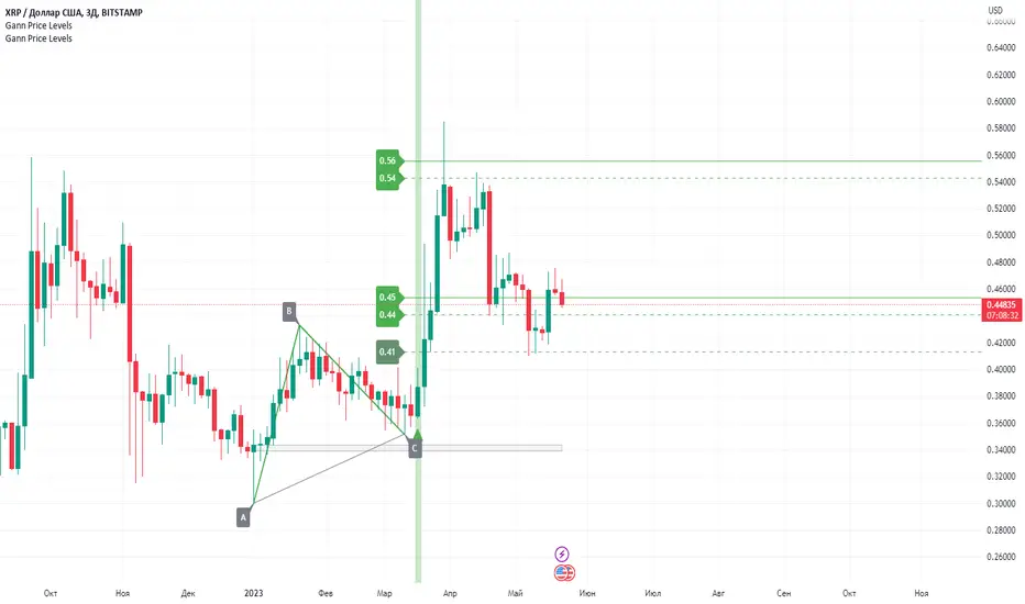
Gann Price LevelsGann Price Level is a powerful indicator based on the methods of the legendary trader William D. Gann. It provides traders with the ability to forecast future targets, both trending and retracement, based on just three anchor points and generates clear entry signals in the form of arrows. This indicator offers broad capabilities that assist traders in making informed decisions and optimizing their trading strategies. Here are a few key features of this indicator:
Calculation of future targets: Gann Price Level allows traders to determine potential price levels that may be reached in the future. It is based on the concept of geometric levels and numerical relationships, making it an effective tool for forecasting future price movements. Its algorithm incorporates geometry, mathematics, and Gann's angular relationships.
Three-point approach: One of the main advantages of Gann Price Level is its ability to work with only three anchor points. Traders need to specify three (ABC) points forming a triangle, and the indicator automatically calculates the target price levels. This simplifies the analysis process and makes it more intuitive.
Entry signals: In addition to forecasting target levels, Gann Price Level provides clear entry signals in the form of arrows. This helps traders identify optimal moments to enter positions, improving the accuracy of their trades.
Timeframes: Gann Price Level can be applied to various time intervals, including both short-term and long-term charts. This allows traders to adapt the indicator to their trading strategies and trade across different markets.
Versatility: Gann Price Level can be used to analyze various financial instruments, including stocks, forex, commodities, cryptocurrencies, and more. This makes it a versatile tool for traders operating in different market segments.
Another key feature of this indicator is the additional level calculation algorithm, which, when working with a trend, forms an optimal gray zone for forming point C, while when calculating retracement levels, it adds an additional magnetic target in the form of a gray zone.
Additionally, traders can combine this indicator with other indicators or chart patterns to obtain more accurate signals and confirmations. Moreover, Gann Price Level works effectively in both upward and downward trends, making it a flexible tool for traders of different trading styles. It can be used to determine potential support and resistance levels, as well as entry and exit points for positions.
Working with this indicator is straightforward. The user needs to select three (ABC) points forming a triangle, and the indicator will automatically calculate the future price targets. An entry arrow will also appear, enabling the user to enter the trade in a timely manner. The stop loss is placed slightly below point C (at the spread distance) for buy trades and above point C (at the spread distance) for sell trades. The first target is represented by a dashed line. Once this target is reached, a portion of the position (usually 50%) is closed, and the stop loss is moved to breakeven. The remaining part of the position is held until subsequent price levels based on personal preferences.
Construction rules:
When calculating targets in an upward trend, point A is below points BC, and point C is always between points AB.
When calculating targets in a downward trend, point A is above points BC, and point C is always between points AB.
When calculating retracement targets in an upward trend, point B is above points AC, point A is always between points BC, and point C is below AB.
When calculating retracement targets in a downward trend, point B is below points AC, point A is always between points BC, and point C is above AB.
This indicator relies entirely on the manual construction of the ABC points by the user.
Inverted ProjectionThe "Inverted Projection" indicator calculates the Simple Moving Average (SMA) and draws lines representing an inverted projection. The indicator swaps the highs and lows of the projection to provide a unique perspective on price movement.
This indicator is a simple study that should not be taken seriously as a tool for predicting future price movements; it is purely intended for exploratory purposes.

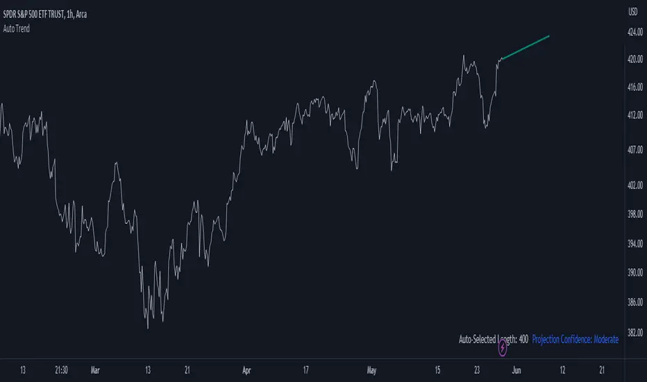
Auto Trend ProjectionAuto Trend Projection is an indicator designed to automatically project the short-term trend based on historical price data. It utilizes a dynamic calculation method to determine the slope of the linear regression line, which represents the trend direction. The indicator takes into account multiple length inputs and calculates the deviation and Pearson's R values for each length.
Using the highest Pearson's R value, Auto Trend Projection identifies the optimal length for the trend projection. This ensures that the projected trend aligns closely with the historical price data.
The indicator visually displays the projected trend using trendlines. These trendlines extend into the future, providing a visual representation of the potential price movement in the short term. The color and style of the trendlines can be customized according to user preferences.
Auto Trend Projection simplifies the process of trend analysis by automating the projection of short-term trends. Traders and investors can use this indicator to gain insights into potential price movements and make informed trading decisions.
Please note that Auto Trend Projection is not a standalone trading strategy but a tool to assist in trend analysis. It is recommended to combine it with other technical analysis tools and indicators for comprehensive market analysis.
Overall, Auto Trend Projection offers a convenient and automated approach to projecting short-term trends, empowering traders with valuable insights into the potential price direction.
Ultimate Trend LineThe "Ultimate Trend Line" indicator, designed for overlay on financial charts, calculates and plots a global trend line. It works by first allowing users to input several parameters such as different lengths for up to 21 groups, a multiplier that defines the deviation from the linear regression line for calculating the upper and lower bands, and a color for the fill.
Using these inputs, it calculates the upper and lower bands for each length group based on a multiple of the standard deviation from the linear regression line. It then averages these bands to define the global trend line, which is plotted on the graph.
Although the code includes commented-out lines for plotting each individual upper and lower band, the indicator as it stands only displays the overall average trend line. The line's color and linewidth can be adjusted according to user preferences.
This indicator can be effectively used on both logarithmic and linear scales. This versatility allows it to be adaptable to various types of financial charts and trading styles, providing a flexible tool for users to assess and visualize trend patterns across different market conditions and time frames. It maintains its accuracy and relevance, regardless of the scale used, thus making it a comprehensive solution for trend line analysis in diverse scenarios.
It's important to note that the "Ultimate Trend Line" indicator requires a substantial amount of historical data to function properly. If insufficient historical data is available, the indicator may not display accurately or at all. This issue is particularly prevalent when using larger time units, such as weekly or monthly charts, where the available data may not stretch back far enough to satisfy the requirements of the indicator. As such, users should ensure they are operating on a time scale and data set that provides adequate historical depth for the reliable operation of this indicator.

TrueLevel BandsTrueLevel Bands is a powerful trading indicator that employs linear regression and standard deviation to create dynamic, envelope-style bands around the price action of a financial instrument. These bands are designed to help traders identify potential support and resistance levels, trend direction, and volatility.
The TrueLevel Bands indicator consists of multiple envelope bands, each constructed using different timeframes or lengths, and a multiple (mult) factor. The multiple factor determines the width of the bands by adjusting the number of standard deviations from the linear regression line.
Key Features of TrueLevel Bands
1. Multi-Timeframe Analysis: Unlike traditional moving average-based indicators, TrueLevel Bands allow traders to incorporate multiple timeframes into their analysis. This helps traders capture both short-term and long-term market dynamics, offering a more comprehensive understanding of price behavior.
2. Customization: The TrueLevel Bands indicator offers a high level of customization, allowing traders to adjust the lengths and multiple factors to suit their trading style and preferences. This flexibility enables traders to fine-tune the indicator to work optimally with various instruments and market conditions.
3. Adaptive Volatility: By incorporating standard deviation, TrueLevel Bands can automatically adjust to changing market volatility. This feature enables the bands to expand during periods of high volatility and contract during periods of low volatility, providing traders with a more accurate representation of market dynamics.
4. Dynamic Support and Resistance Levels: TrueLevel Bands can help traders identify dynamic support and resistance levels, as the bands adjust in real-time according to price action. This can be particularly useful for traders looking to enter or exit positions based on support and resistance levels.
5. The "Global Trend Line" refers to the average of the bands used to indicate the overall trend.
Why TrueLevel Bands are Different from Classic Moving Averages
TrueLevel Bands differ from conventional moving averages in several ways:
1. Linear Regression: While moving averages are based on simple arithmetic means, TrueLevel Bands use linear regression to determine the centerline. This offers a more accurate representation of the trend and helps traders better assess potential entry and exit points.
2. Envelope Style Bands: Unlike moving averages, which are single lines, TrueLevel Bands form envelope-style bands around the price action. This provides traders with a visual representation of potential support and resistance levels, trend direction, and volatility.
3. Multi-Timeframe Analysis: Classic moving averages typically focus on a single timeframe. In contrast, TrueLevel Bands incorporate multiple timeframes, enabling traders to capture a broader understanding of market dynamics.
4. Adaptive Volatility: Traditional moving averages do not account for changing market volatility, whereas TrueLevel Bands automatically adjust to volatility shifts through the use of standard deviation.
The TrueLevel Bands indicator is a powerful, versatile tool that offers traders a unique approach to technical analysis. With its ability to adapt to changing market conditions, provide multi-timeframe analysis, and dynamic support and resistance levels, TrueLevel Bands can serve as an invaluable asset to both novice and experienced traders looking to gain an edge in the markets.
