Position resetThe "Position Reset" indicator
The Position Reset indicator is a sophisticated technical analysis tool designed to identify possible entry points into short positions based on an analysis of market volatility and the behavior of various groups of bidders. The main purpose of this indicator is to provide traders with information about the current state of the market and help them decide whether to open short positions depending on the level of volatility and the mood of the main players.
The main components of the indicator:
1. Parameters for the RSI (Relative Strength Index):
The indicator uses two sets of parameters to calculate the RSI: one for bankers ("Banker"), the other for hot money ("Hot Money").
RSI for Bankers:
RSIBaseBanker: The baseline for calculating bankers' RSI. The default value is 50.
RSIPeriodBanker: The period for calculating the RSI for bankers. The default period is 14.
RSI for hot money:
RSIBaseHotMoney: The baseline for calculating the RSI of hot money. The default value is 30.
RSIPeriodHotMoney: The period for calculating the RSI for hot money. The default period is 21.
These parameters allow you to adjust the sensitivity of the indicator to the actions of different groups of market participants.
2. Sensitivity:
Sensitivity determines how strongly changes in the RSI will affect the final result of calculations. It is configured separately for bankers and hot money:
SensitivityBanker: Sensitivity for bankers' RSI. It is set to 2.0 by default.
SensitivityHotMoney: Sensitivity for hot money RSI. It is set to 1.0 by default.
Changing these parameters allows you to adapt the indicator to different market conditions and trader preferences.
3. Volatility Analysis:
Volatility is measured based on the length of the period, which is set by the volLength parameter. The default length is 30 candles. The indicator calculates the difference between the highest and lowest value for the specified period and divides this difference by the lowest value, thus obtaining the volatility coefficient.
Based on this coefficient, four levels of volatility are distinguished.:
Extreme volatility: The coefficient is greater than or equal to 0.25.
High volatility: The coefficient ranges from 0.125 to 0.2499.
Normal volatility: The coefficient ranges from 0.05 to 0.1249.
Low volatility: The coefficient is less than 0.0499.
Each level of volatility has its own significance for making decisions about entering a position.
4. Calculation functions:
The indicator uses several functions to process the RSI and volatility data.:
rsi_function: This function applies to every type of RSI (bankers and hot money). It adjusts the RSI value according to the set sensitivity and baseline, limiting the range of values from 0 to 20.
Moving Averages: Simple moving averages (SMA), exponential moving averages (EMA), and weighted moving averages (RMA) are used to smooth fluctuations. They are applied to different time intervals to obtain the average values of the RSI.
Thus, the indicator creates a comprehensive picture of market behavior, taking into account both short-term and long-term dynamics.
5. Bearish signals:
Bearish signals are considered situations when the RSI crosses certain levels simultaneously with a drop in indicators for both types of market participants (bankers and hot money).:
The bankers' RSI crossing is below the level of 8.5.
The current hot money RSI is less than 18.
The moving averages for banks and hot money are below their signal lines.
The RSI values for bankers are less than 5.
These conditions indicate a possible beginning of a downtrend.
6. Signal generation:
Depending on the current level of volatility and the presence of bearish signals, the indicator generates three types of signals:
Orange circle: Extremely high volatility and the presence of a bearish signal.
Yellow circle: High volatility and the presence of a bearish signal.
Green circle: Low volatility and the presence of a bearish signal.
These visual markers help the trader to quickly understand what level of risk accompanies each specific signal.
7. Notifications:
The indicator supports the function of sending notifications when one of the three types of signals occurs. The notification contains a brief description of the conditions under which the signal was generated, which allows the trader to respond promptly to a change in the market situation.
Advantages of using the "Position Reset" indicator:
Multi-level analysis: The indicator combines technical analysis (RSI) and volatility assessment, providing a comprehensive view of the current market situation.
Flexibility of settings: The ability to adjust the sensitivity parameters and the RSI baselines allows you to adapt the indicator to any market conditions and personal preferences of the trader.
Clear visualization: The use of colored labels on the chart simplifies the perception of information and helps to quickly identify key points for entering a trade.
Notification support: The notification sending feature makes it much easier to monitor the market, allowing you to respond to important events in time.
Cerca negli script per "averages"

Waldo's RSI Color Trend Candles
TradingView Description for Waldo's RSI Color Trend Candles
Title: Waldo's RSI Color Trend Candles
Short Title: Waldo RSI CTC
Overview:
Waldo's RSI Color Trend Candles is a visually intuitive indicator designed to enhance your trading experience by color-coding candlesticks based on the integration of Relative Strength Index (RSI) momentum and moving average trend analysis. This innovative tool overlays directly on your price chart, providing a clear, color-based representation of market sentiment and trend direction.
What is it?
This indicator combines the power of RSI with the simplicity of moving averages to offer traders a unique way to visualize market conditions:
RSI Integration: The RSI is computed with customizable parameters, allowing traders to adjust how momentum is interpreted. The RSI values influence the primary color of the candles, indicating overbought or oversold market states.
Moving Averages: Utilizing two Simple Moving Averages (SMAs) with user-defined lengths, the indicator helps in identifying trend directions through their crossovers. The fast MA and slow MA can be toggled on/off for visual clarity.
Color Trend Candles: The 'Color Trend Candles' feature uses a dynamic color scheme to reflect different market conditions:
Purple for overbought conditions when RSI exceeds the set threshold (default 70).
Blue for oversold conditions when RSI falls below the set threshold (default 44).
Green indicates a bullish trend, confirmed by both price action and RSI being bullish (fast MA crossing above slow MA, with price above the slow MA).
Red signals a bearish trend, when both price and RSI are bearish (fast MA crossing below slow MA, with price below the slow MA).
Gray for neutral or mixed market sentiment, where signals are less clear or contradictory.
How to Use It:
Waldo's RSI Color Trend Candles is tailored for traders who appreciate visual cues in their trading strategy:
Trend and Momentum Insight: The color of each candle gives an immediate visual representation of both the trend (via MA crossovers) and momentum (via RSI). Green and red candles align with bullish or bearish trends, respectively, providing a quick reference for market direction.
Identifying Extreme Conditions: Purple and blue candles highlight potential reversal zones or areas where the market might be overstretched, offering opportunities for contrarian trades or to anticipate market corrections.
Customization: Users can adjust the RSI length, overbought/oversold levels, and the lengths of the moving averages to align with their trading style or the specific characteristics of the asset they're trading.
This customization ensures the indicator can be tailored to various market conditions.
Simplified Decision Making: Designed for traders who prefer a visual approach, this indicator simplifies the decision-making process by encoding complex market data into an easy-to-understand color system.
However, for a robust trading strategy, it's recommended to use it alongside other analytical tools.
Control Over Display: The option to show or hide moving averages and to enable or disable the color-coding of candles provides users with control over how information is presented, allowing for a cleaner chart or more detailed analysis as preferred.
Conclusion:
Waldo's RSI Color Trend Candles offers a fresh, visually appealing method to interpret market trends and momentum through the color of candlesticks. It's ideal for traders looking for a straightforward way to gauge market sentiment at a glance. While this indicator can significantly enhance your trading setup, remember to incorporate it within a broader strategy, using additional confirmation from other indicators or analysis methods to manage risk and validate trading decisions. Dive into the colorful world of trading with Waldo's RSI Color Trend Candles and let the market's mood guide your trades with clarity and ease.
Volume ComparisonThis indicator is designed to visually compare the current day's trading volume against the average trading volumes of 3, 5, and 10 days. It highlights certain conditions based on the comparison and provides alerts.
Inputs for Customization:
1. The user can toggle visibility for the 3-day, 5-day, and 10-day average volumes using boolean inputs.
2. Average Volume Calculation:
This indicator calculate simple moving averages of the trading volume for 3, 5, and 10-day periods.
3.Conditions:
The indicator checks whether the current day's volume is greater than the respective moving averages for 3, 5, and 10 days.
4. Background Color for Visual Indicators:
If the current day's volume is greater than any of the averages and the corresponding option is enabled, the background color is adjusted:
* Green if the volume is greater than the 3-day average.
* Blue if the volume is greater than the 5-day average.
* Red if the volume is greater than the 10-day average.
5. Plotting the Averages:
The moving averages are plotted on the chart, with different colors for each (green for 3-day, blue for 5-day, and red for 10-day).
6. This indicator can be used to help visually track whether today's volume is above the moving average, which can signal increased market activity or interest.

Dashboard MTF profile volume Indicator Description
This indicator, titled "Swing Points and Liquidity & Profile Volume," combines multiple features to provide a comprehensive market analysis:
Volume Profile: Displays buy and sell volumes across multiple timeframes (1 minute, 5 minutes, 15 minutes, 1 hour, 4 hours, 1 day).
Volume Moving Averages: Plots two moving averages (short and long) to analyze volume trends.
Dashboard: A summary dashboard shows buy and sell volumes for each timeframe, with distinct colors for better visualization.
Swing Points: Identifies liquidity levels and swing points to help pinpoint key entry and exit zones.
How to Use
1. Indicator Installation
Go to TradingView.
Open the Pine Script Editor.
Copy and paste the provided code.
Click on "Add to Chart."
2. Indicator Settings
The indicator offers several customizable parameters:
Display Volume (1 minute, 5 minutes, 15 minutes, 1 hour, 4 hours, 1 day): Enable or disable volume display for each timeframe.
Short Moving Average Length (MA): Set the short moving average period (default: 5).
Long Moving Average Length (MA): Set the long moving average period (default: 14).
Dashboard Position: Choose where to display the dashboard (bottom-right, bottom-left, top-right, top-left).
Text Color: Customize the text color in the dashboard.
Text Size: Choose text size (small, normal, large).
3. Using the Indicator
Volume Analysis
The dashboard displays buy (Buy Volume) and sell (Sell Volume) volumes for each timeframe.
Buy Volume: Volume of trades where the closing price is higher than the opening price (aggressive buying).
Sell Volume: Volume of trades where the closing price is equal to or lower than the opening price (aggressive selling).
Volumes are displayed in real-time and update with each new candle.
Volume Moving Averages
Two moving averages are plotted on the chart:
MA Volume (Short): Short moving average (blue) to identify short-term volume trends.
MA Volume (Long): Long moving average (red) to identify long-term volume trends.
Use these moving averages to spot accumulation or distribution periods.
Swing Points and Liquidity
Swing points are identified based on price levels where volumes are highest.
These levels can act as support/resistance zones or liquidity areas to plan entries and exits.
Usage Guidelines
1. Entering a Position
Buy (Long):
When Buy Volume is significantly higher than Sell Volume across multiple timeframes.
When the short moving average (blue) crosses above the long moving average (red).
Sell (Short):
When Sell Volume is significantly higher than Buy Volume across multiple timeframes.
When the short moving average (blue) crosses below the long moving average (red).
2. Exiting a Position
Use liquidity levels (swing points) to set profit targets or stop-loss levels.
Monitor volume changes to anticipate trend reversals.
3. Risk Management
Use stop-loss orders to limit losses.
Avoid trading during low-volume periods to reduce false signals.
Compliance with Trading View Guidelines
Intellectual Property:
The code is provided for educational and personal use. You may modify and use it but cannot resell or distribute it as your own work.
Responsible Use:
Trading View encourages responsible use of indicators. Test the indicator on a demo account before using it in live trading.
Transparency:
The code is fully transparent and can be reviewed in the Pine Script Editor. You may modify it to suit your needs.
Practical Examples
Scenario 1: Bullish Trend
Buy Volume is high on 1-hour and 4-hour time frames.
The short moving average (blue) is above the long moving average (red).
Action: Open a long position (Buy) and set a stop-loss below the last swing low.
Scenario 2: Bearish Trend
Sell Volume is high on 1-hour and 4-hour time frames.
The short moving average (blue) is below the long moving average (red).
Action: Open a short position (Sell) and set a stop-loss above the last swing high.

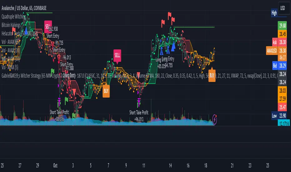
Gabriel's Witcher Strategy [65 Minute Trading Bot]Strategy Description: Gabriel's Witcher Strategy
Author: Gabriel
Platform: TradingView Pine Script (Version 5)
Backtested Asset: Avalanche (Coinbase Brokage for Volume adjustment)
Timeframe: 65 Minutes
Strategy Type: Comprehensive Trend-Following and Momentum Strategy with Scalping and Risk Management Features
Overview
Gabriel's Witcher Strategy is an advanced trading bot designed for the Avalanche pair on a 65-minute timeframe. This strategy integrates a multitude of technical indicators to identify and execute high-probability trading opportunities. By combining trend-following, momentum, volume analysis, and range filtering, the strategy aims to capitalize on both long and short market movements. Additionally, it incorporates scalping mechanisms and robust risk management features, including take-profit (TP) levels and commission considerations, to optimize trade performance and profitability.
====Key Components====
Source Selection:
Custom Source Flexibility: Allows traders to select from a wide range of price and volume sources (e.g., Close, Open, High, Low, HL2, HLC3, OHLC4, VWAP, On-Balance Volume, etc.) for indicator calculations, enhancing adaptability to various trading styles.
Various curves of Volume Analysis are employed:
Tick Volume Calculation: Utilizes tick volume as a fallback when actual volume data is unavailable, ensuring consistency across different data feeds.
Volume Indicators: Incorporates multiple volume-based indicators such as On-Balance Volume (OBV), Accumulation/Distribution (AccDist), Negative Volume Index (NVI), Positive Volume Index (PVI), and Price Volume Trend (PVT) for comprehensive market analysis.
Trend Indicators:
ADX (Average Directional Index): Measures trend strength using either the Classic or Masanakamura method, with customizable length and threshold settings. It's used to open positions when the mesured trend is strong, or exit when its weak.
Jurik Moving Average (JMA): A smooth moving average that reduces lag, configurable with various parameters including source, resolution, and repainting options.
Parabolic SAR: Identifies potential reversals in market trends with adjustable start, increment, and maximum settings.
Custom Trend Indicator: Utilizes highest and lowest price points over a specified timeframe to determine current and previous trend bases, visually represented with color-filled areas.
Momentum Indicators:
Relative Strength Index (RSI): Evaluates the speed and change of price movements, smoothed with a custom length and source. It's used to not enter the market for shorts in oversold or longs for overbought conditions, and to enter for long in oversold or shorts for overboughts.
Momentum-Based Calculations: Employs both Double Exponential Moving Averages (DEMA) on a MACD-based RSI to enhance momentum signal accuracy which is then further accelerated by a Hull MA. This is the technical analysis tool that determines bearish or bullish momentum.
OBV-Based Momentum Conditions: Uses two exponential moving averages of OBV to determine bullish or bearish momentum shifts, anomalities, breakouts where banks flow their funds in or Smart Money Concepts trade.
Moving Averages (MA):
Multiple MA Types: Includes Simple Moving Average (SMA), Exponential Moving Average (EMA), Weighted Moving Average (WMA), Hull Moving Average (HMA), and Volume-Weighted Moving Average (VWMA), selectable via input parameters.
MA Speed Calculation: Measures the percentage change in MA values to determine the direction and speed of the trend.
Range Filtering:
Variance-Based Filter: Utilizes variance and moving averages to filter out trades during low-volatility periods, enhancing trade quality.
Color-Coded Range Indicators: Visualizes range filtering with color changes on the chart for quick assessment.
Scalping Mechanism:
Heikin-Ashi Candles: Optionally uses Heikin-Ashi candles for smoother price action analysis.
EMA-Based Trend Detection: Employs fast, medium, and slow EMAs to determine trend direction and potential entry points.
Fractal-Based Filtering: Detects regular or BW (Black & White) fractals to confirm trade signals.
Take Profit (TP) Management:
Dynamic TP Levels: Calculates TP levels based on the number of consecutive long or short entries, adjusting targets to maximize profits.
TP Signals and Re-Entry: Plots TP signals on the chart and allows for automatic re-entry upon TP hit, maintaining continuous trade flow.
Risk Management:
Commission Integration: Accounts for trading commissions to ensure net profitability.
Position Sizing: Configured to use a percentage of equity for each trade, adjustable via input parameters.
Pyramiding: Allows up to one additional position per direction to enhance gains during strong trends.
Alerts and Visual Indicators:
Buy/Sell Signals: Plots visual indicators (triangles and flags) on the chart to signify entry and TP points.
Bar Coloring: Changes bar colors based on ADX and trend conditions for immediate visual cues.
Price Levels: Marks significant price levels related to TP and position entries with cross styles.
Input Parameters
Source Settings:
Custom Sources (srcinput): Choose from various price and volume sources to tailor indicator calculations.
ADX Settings:
ADX Type (ADX_options): Select between 'CLASSIC' and 'MASANAKAMURA' methods.
ADX Length (ADX_len): Defines the period for ADX calculation.
ADX Threshold (th): Sets the minimum ADX value to consider a strong trend.
RSI Settings:
RSI Length (len_3): Period for RSI calculation.
RSI Source (src_3): Source data for RSI.
Trend Strength Settings:
Channel Length (n1): Period for trend channel calculation.
Average Length (n2): Period for smoothing trend strength.
Jurik Moving Average (JMA) Settings:
JMA Source (inp): Source data for JMA.
JMA Resolution (reso): Timeframe for JMA calculation.
JMA Repainting (rep): Option to allow JMA to repaint.
JMA Length (lengths): Period for JMA.
Parabolic SAR Settings:
SAR Start (start): Initial acceleration factor.
SAR Increment (increment): Acceleration factor increment.
SAR Maximum (maximum): Maximum acceleration factor.
SAR Point Width (width): Visual width of SAR points.
Trend Indicator Settings:
Trend Timeframe (timeframe): Period for trend indicator calculations.
Momentum Settings:
Source Type (srcType): Select between 'Price' and 'VWAP'.
Momentum Source (srcPrice): Source data for momentum calculations.
RSI Length (rsiLen): Period for momentum RSI.
Smooth Length (sLen): Smoothing period for momentum RSI.
OBV Settings:
OBV Line 1 (e1): EMA period for OBV line 1.
OBV Line 2 (e2): EMA period for OBV line 2.
Moving Average (MA) Settings:
MA Length (length): Period for MA calculations.
MA Type (matype): Select MA type (1: SMA, 2: EMA, 3: HMA, 4: WMA, 5: VWMA).
Range Filter Settings:
Range Filter Length (length0): Period for range filtering.
Range Filter Multiplier (mult): Multiplier for range variance.
Take Profit (TP) Settings:
TP Long (tp_long0): Percentage for long TP.
TP Short (tp_short0): Percentage for short TP.
Scalping Settings:
Scalping Activation (ACT_SCLP): Enable or disable scalping.
Scalping Length (HiLoLen): Period for scalping indicators.
Fast EMA Length (fastEMAlength): Period for fast EMA in scalping.
Medium EMA Length (mediumEMAlength): Period for medium EMA in scalping.
Slow EMA Length (slowEMAlength): Period for slow EMA in scalping.
Filter (filterBW): Enable or disable additional fractal filtering.
Pullback Lookback (Lookback): Number of bars for pullback consideration.
Use Heikin-Ashi Candles (UseHAcandles): Option to use Heikin-Ashi candles for smoother trend analysis.
Strategy Logic
Indicator Calculations:
Volume and Source Selection: Determines the primary data source based on user input, ensuring flexibility and adaptability.
ADX Calculation: Computes ADX using either the Classic or Masanakamura method to assess trend strength.
RSI Calculation: Evaluates market momentum using RSI, further smoothed with custom periods.
Trend Strength Assessment: Utilizes trend channel and average lengths to gauge the robustness of current trends.
Jurik Moving Average (JMA): Smooths price data to reduce lag and enhance trend detection.
Parabolic SAR: Identifies potential trend reversals with adjustable parameters for sensitivity.
Momentum Analysis: Combines RSI with DEMA and OBV-based conditions to confirm bullish or bearish momentum.
Moving Averages: Employs multiple MA types to determine trend direction and speed.
Range Filtering: Filters out low-volatility periods to focus on high-probability trades.
Trade Conditions:
Long Entry Conditions:
ADX Confirmation: ADX must be above the threshold, indicating a strong uptrend.
RSI and Momentum: RSI below 70 and positive momentum signals.
JMA and SAR: JMA indicates an uptrend, and Parabolic SAR is below the price.
Trend Indicator: Confirms the current trend direction.
Range Filter: Ensures market is in an upward range.
Scalping Option: If enabled, additional scalping conditions must be met.
Short Entry Conditions:
ADX Confirmation: ADX must be above the threshold, indicating a strong downtrend.
RSI and Momentum: RSI above 30 and negative momentum signals.
JMA and SAR: JMA indicates a downtrend, and Parabolic SAR is above the price.
Trend Indicator: Confirms the current trend direction.
Range Filter: Ensures market is in a downward range.
Scalping Option: If enabled, additional scalping conditions must be met.
Position Management:
Entry Execution: Places long or short orders based on the identified conditions and user-selected position types (Longs, Shorts, or Both).
Take Profit (TP): Automatically sets TP levels based on predefined percentages, adjusting dynamically with consecutive trades.
Re-Entry Mechanism: Allows for automatic re-entry upon TP hit, maintaining active trading positions.
Exit Conditions: Closes positions when TP levels are reached or when opposing trend signals are detected.
Visual Indicators:
Bar Coloring: Highlights bars in green for bullish conditions, red for bearish, and orange for neutral.
Plotting Price Levels: Marks significant price levels related to TP and trade entries with cross symbols.
Signal Shapes: Displays triangle and flag shapes on the chart to indicate trade entries and TP hits.
Alerts:
Custom Alerts: Configured to notify traders of long entries, short entries, and TP hits, enabling timely trade management and execution.
Usage Instructions
Setup:
Apply the Strategy: Add the script to your TradingView chart set to BTCUSDT with a 65-minute timeframe.
Configure Inputs: Adjust the input parameters under their respective groups (e.g., Source Settings, ADX, RSI, Trend Strength, etc.) to match your trading preferences and risk tolerance.
Position Selection:
Choose Position Type: Use the Position input to select Longs, Shorts, or Both based on your market outlook.
Execution: The strategy will automatically execute and manage positions according to the selected type, ensuring targeted trading actions.
Signal Interpretation:
Buy Signals: Blue triangles below the bars indicate potential long entry points.
Sell Signals: Red triangles above the bars indicate potential short entry points.
Take Profit Signals: Flags above or below the bars signify TP hits for long and short positions, respectively.
Bar Colors: Green bars suggest bullish conditions, red bars indicate bearish conditions, and orange bars represent neutral or consolidating markets.
Risk Management:
Default Position Size: Set to 100% of equity. Adjust the default_qty_value as needed for your risk management strategy.
Commission: Accounts for a 0.1% commission per trade. Adjust the commission_value to match your broker's fees.
Pyramiding: Allows up to one additional position per direction to enhance gains during strong trends.
Backtesting and Optimization:
Historical Testing: Utilize TradingView's backtesting features to evaluate the strategy's performance over historical data.
Parameter Tuning: Optimize input parameters to align the strategy with current market dynamics and personal trading objectives.
Alerts Configuration:
Set Up Alerts: Enable and configure alerts based on the predefined alertcondition statements to receive real-time notifications of trade signals and TP hits.
Additional Features
Comprehensive Indicator Integration: Combines multiple technical indicators to provide a holistic view of market conditions, enhancing trade signal accuracy.
Scalping Options: Offers an optional scalping mechanism to capitalize on short-term price movements, increasing trading flexibility.
Dynamic Take Profit Levels: Adjusts TP targets based on the number of consecutive trades, maximizing profit potential during favorable trends.
Advanced Volume Analysis: Utilizes various volume indicators to confirm trend strength and validate trade signals.
Customizable Range Filtering: Filters trades based on market volatility, ensuring trades are taken during optimal conditions.
Heikin-Ashi Candle Support: Optionally uses Heikin-Ashi candles for smoother price action analysis and reduced noise.
====Recommendations====
Thorough Backtesting:
Historical Performance: Before deploying the strategy in a live trading environment, perform comprehensive backtesting to understand its performance under various market conditions. These are the premium settings for Avalanche Coinbase.
Optimization: Regularly review and adjust input parameters to ensure the strategy remains effective amidst changing market volatility and trends. Backtest the strategy for each crypto and make sure you are in the right brokage when using the volume sources as it will affect the overall outcome of the trading strategy.
Risk Management:
Position Sizing: Adjust the default_qty_value to align with your risk tolerance and account size.
Stop-Loss Implementation: Although the strategy includes TP levels, they're also consided to be a stop-loss mechanisms to protect against adverse market movements.
Commission Adjustment: Ensure the commission_value accurately reflects your broker's fees to maintain realistic backtesting results. Generally, 0.1~0.3% are most of the average broker's comission fees.
Slipage: The slip comssion is 1 Tick, since the strategy is adjusted to only enter/exit on bar close where most positions are available.
Continuous Monitoring:
Strategy Performance: Regularly monitor the strategy's performance to ensure it operates as expected and make adjustments as needed. A max-drawndown hit has been added to operate in case the premium Avalanche settings go wrong, but you can turn it off an adjust the equity percentage to 50% if you are confortable with the high volatile max-drown or even 100% if your account allows you to borrow cash.
Customization:
Indicator Parameters: Tailor indicator settings (e.g., ADX length, RSI period, MA types) to better fit your specific trading style and market conditions.
Scalping Options: Enable or disable scalping based on your trading preferences and risk appetite.
Conclusion
Gabriel's Witcher Strategy is a robust and versatile trading solution designed to navigate the complexities of the Crypto market. By integrating a wide array of technical indicators and providing extensive customization options, this strategy empowers traders to execute informed and strategic trades. Its comprehensive approach, combining trend analysis, momentum detection, volume evaluation, and range filtering, ensures that trades are taken during optimal market conditions. Additionally, the inclusion of scalping features and dynamic take-profit management enhances the strategy's adaptability and profitability potential. Unlike any trading strategy, with both diligent testing and continuous monitoring under the strategy tester, it's possible to achieve sustained success by adjusting the settings to the individual Crypto that need it, for example this one is preset for Avalanche Coinbase 65 Miinutes but it can be adjust for BTCUSD or Etherium if you backtest and search for the right settings.
MVSF 6.0[ELPANO]The "MVSF 6.0 " indicator, which stands for Multi-Variable Strategy Framework, overlays on price charts to aid in trading decisions. It combines various moving averages and volume data to generate buy and sell signals based on predefined conditions.
Key features of the indicator include:
Moving Averages: It uses three exponential moving averages (EMAs) with lengths of 200, 100, and 50, and two simple moving averages (SMAs) with lengths of 14 and 9. These averages are combined into a single average line to detect trends.
Volume Analysis: The volume is assessed over a specified period (default is 2 bars) to determine its trend relative to its average, influencing the color and interpretation of signals.
Price Source and VWAP: Users can select the price (close, low, or high) used for calculations. The volume-weighted average price (VWAP) serves as a potential benchmark or condition in signal generation.
Signal Generation: Buy and sell signals are based on the relationship of the price to the average line and VWAP, the direction of the last candle, and the trend direction of the average line. These signals are visually represented on the chart.
Customization: Traders can toggle the visibility of signals, entry points, the average line, and even use these elements as conditions for filtering signals.
This script is designed to be flexible, allowing traders to modify settings according to their strategy needs. The description and implementation aim to provide clarity on how each component works together to assist in trading decisions, adhering to best practices for creating and publishing trading scripts.
*************************************
Der Indikator "MVSF 6.0 ", der für Multi-Variable Strategy Framework steht, wird über Preisdiagramme gelegt, um bei Handelsentscheidungen zu helfen. Er kombiniert verschiedene gleitende Durchschnitte und Volumendaten, um Kauf- und Verkaufssignale basierend auf vordefinierten Bedingungen zu generieren.
Wesentliche Merkmale des Indikators umfassen:
Gleitende Durchschnitte: Es werden drei exponentielle gleitende Durchschnitte (EMAs) mit Längen von 200, 100 und 50 sowie zwei einfache gleitende Durchschnitte (SMAs) mit Längen von 14 und 9 verwendet. Diese Durchschnitte werden zu einer einzelnen Durchschnittslinie kombiniert, um Trends zu erkennen.
Volumenanalyse: Das Volumen wird über einen festgelegten Zeitraum (standardmäßig 2 Balken) bewertet, um seinen Trend im Vergleich zum Durchschnitt zu bestimmen, was die Farbe und Interpretation der Signale beeinflusst.
Preisquelle und VWAP: Benutzer können den für Berechnungen verwendeten Preis (Schluss-, Tief- oder Hochkurs) auswählen. Der volumengewichtete Durchschnittspreis (VWAP) dient als mögliche Benchmark oder Bedingung bei der Generierung von Signalen.
Signalgenerierung: Kauf- und Verkaufssignale basieren auf dem Verhältnis des Preises zur Durchschnittslinie und zum VWAP, der Richtung der letzten Kerze und der Trendrichtung der Durchschnittslinie. Diese Signale werden visuell auf dem Diagramm dargestellt.
Anpassung: Händler können die Sichtbarkeit von Signalen, Einstiegspunkten, der Durchschnittslinie und sogar deren Verwendung als Bedingungen für die Filterung von Signalen ein- und ausschalten.
Dieses Skript ist so konzipiert, dass es flexibel ist und Händlern erlaubt, die Einstellungen gemäß ihren Strategiebedürfnissen zu modifizieren. Die Beschreibung und Implementierung zielen darauf ab, Klarheit darüber zu schaffen, wie jede Komponente zusammenarbeitet, um bei Handelsentscheidungen zu helfen, und halten sich an die besten Praktiken für die Erstellung und Veröffentlichung von Handelsskripten.

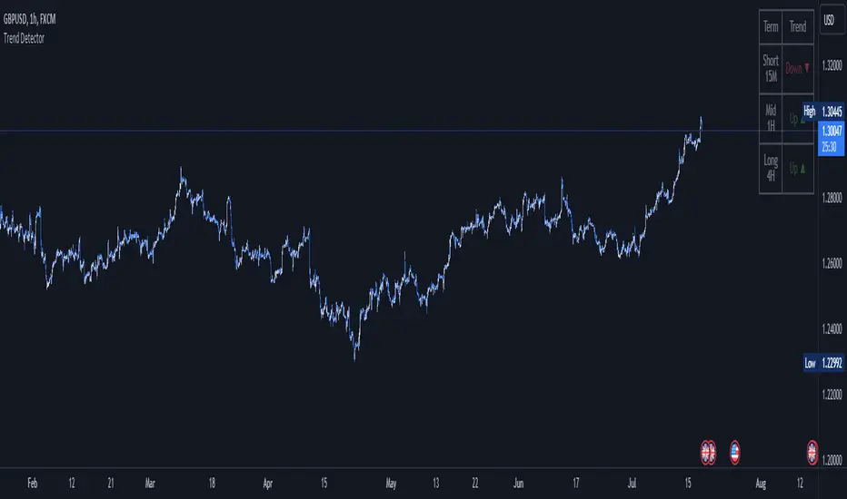
Trend DetectorThe Trend Detector indicator is a powerful tool to help traders identify and visualize market trends with ease. This indicator uses multiple moving averages (MAs) of different timeframes to provide a comprehensive view of market trends, making it suitable for traders of all experience levels.
█ USAGE
This indicator will automatically plot the chosen moving averages (MAs) on your chart, allowing you to visually assess the trend direction. Additionally, a table displaying the trend data for each selected MA timeframe is included to provide a quick overview.
█ FEATURES
1. Customizable Moving Averages: The indicator supports various types of moving averages, including Simple (SMA) , Exponential (EMA) , Smoothed (RMA) , Weighted (WMA) , and Volume-Weighted (VWMA) . You can select the type and length for each MA.
2. Multiple Timeframes: Plot moving averages for different timeframes on a single chart, including fast (short-term) , mid (medium-term) , and slow (long-term) MAs.
3. Trend Detector Table: A customizable table displays the trend direction (Up or Down) for each selected MA timeframe, providing a quick and easy way to assess the market's overall trend.
4. Customizable Appearance: Adjust the colors, frame, border, and text of the Trend Detector Table to match your chart's style and preferences.
5. Wait for Timeframe Close: Option to wait until the selected timeframe closes to plot the MA, which will remove the gaps.
█ CONCLUSION
The Trend Detector indicator is a versatile and user-friendly tool designed to enhance your trading strategy. By providing a clear visualization of market trends across multiple timeframes, this indicator helps you make informed trading decisions with confidence and trade with the market trend. Whether you're a day trader or a long-term investor, this indicator is an essential addition to your trading toolkit.
█ IMPORTANT
This indicator is a tool to aid in your analysis and should not be used as the sole basis for trading decisions. It is recommended to use this indicator in conjunction with other tools and perform comprehensive market analysis before making any trades.
Happy trading!
Uptrick: MultiMA_VolumePurpose:
The "Uptrick: MultiMA_Volume" indicator, identified by its abbreviated title 'MMAV,' is meticulously designed to provide traders with a comprehensive view of market dynamics by incorporating multiple moving averages (MAs) and volume analysis. With adjustable inputs and customizable visibility options, traders can tailor the indicator to their specific trading preferences and strategies, thereby enhancing its utility and usability.
Explanation:
Input Variables and Customization:
Traders have the flexibility to adjust various parameters, including the lengths of different moving averages (SMA, EMA, WMA, HMA, and KAMA), as well as the option to show or hide each moving average and volume-related components.
Customization options empower traders to fine-tune the indicator according to their trading styles and market preferences, enhancing its adaptability across different market conditions.
Moving Averages and Trend Identification:
The script computes multiple types of moving averages, including Simple (SMA), Exponential (EMA), Weighted (WMA), Hull (HMA), and Kaufman's Adaptive (KAMA), allowing traders to assess trend directionality and strength from various perspectives.
Traders can determine potential price movements by observing the relationship between the current price and the plotted moving averages. For example, prices above the moving averages may suggest bullish sentiment, while prices below could indicate bearish sentiment.
Volume Analysis:
Volume analysis is integrated into the indicator, enabling traders to evaluate volume dynamics alongside trend analysis.
Traders can identify significant volume spikes using a customizable threshold, with bars exceeding the threshold highlighted to signify potential shifts in market activity and liquidity.
Determining Potential Price Movements:
By analyzing the relationship between price and the plotted moving averages, traders can infer potential price movements.
Bullish biases may be suggested when prices are above the moving averages, accompanied by rising volume, while bearish biases may be indicated when prices are below the moving averages, with declining volume reinforcing the potential for downward price movements.
Utility and Potential Usage:
The "Uptrick: MultiMA_Volume" indicator serves as a comprehensive tool for traders, offering insights into trend directionality, strength, and volume dynamics.
Traders can utilize the indicator to identify potential trading opportunities, confirm trend signals, and manage risk effectively.
By consolidating multiple indicators into a single chart, the indicator streamlines the analytical process, providing traders with a concise overview of market conditions and facilitating informed decision-making.
Through its customizable features and comprehensive analysis, the "Uptrick: MultiMA_Volume" indicator equips traders with actionable insights into market trends and volume dynamics. By integrating trend analysis and volume assessment into their trading strategies, traders can navigate the markets with confidence and precision, thereby enhancing their trading outcomes.

S__Trader's Portfolio ManagementThis custom TradingView script is a powerful tool designed to help investors effectively manage their portfolios. This script allows you to monitor, analyze, and optimize your portfolio performance using moving averages in technical analysis. This script is for the traders who want to manage his portfolio by moving averages which is powered by using 4 of them together.
Timeframe is based on Daily as default but you can prefer to see weekly, monthly or else depends on your trading character
This script uses 4 customizable moving averages to decide cash/stocks ratio. Each moving average has %25 power of decide. If price is above the moving average, each moving average adds %25 to stock total percentage, else below they add %25 to cash. So you can decide your cash stock ratio by that moving averages.
For example if price is above all of that moving averages, script table shows you %100 total for stocks but if price is above for example 2 of that moving averages, script table shows you %50 for stocks and get remaining %50 cash.
For example if price is above only 1 of that moving averages, script table shows %25 for that stocks and that means %75 cash.
If price is below all that moving averages, script table shows %0, means that sell all stocks and stay cash %100
You can choose to plot moving averages or not
Or you can choose just track them by line
You can hide table also and decide table size and place at graph
By using this script, you can monitor your portfolio's performance, manage risk, and optimize your investment strategies. However, please remember that this script is just a tool and should not be used as a sole decision-making tool for investments. Always use it in conjunction with risk management and other analytical methods.
Hopefully, this script will help you enhance your investment process. Best of luck!

VCC SmtmWorks better for Cryptos (1W and greater than) timeframes.
This strategy incorporates multiple indicators to make informed trading signals. It leverages the Stochastic indicator to assess price momentum, utilizes the Bollinger Band to identify potential oversold and overbought conditions, and closely monitors Moving Averages to gauge the trend's bullish or bearish nature.
A long signal will be displayed if the following conditions are met:
The Stochastic D and Stochastic K both indicate an oversold condition, with Stochastic K being lower than Stochastic D.
The current Price Low is below the Bollinger Lower Band.
The Price Close is currently below all Moving Averages.
A Death Cross pattern has formed among the Moving Averages.
A short signal will be displayed if the opposite of the long conditions are true:
The Stochastic D and Stochastic K both indicate an overbought condition, with Stochastic K being higher than Stochastic D.
The current Price High is above the Bollinger Upper Band.
The Price Close is currently above all Moving Averages.
A Golden Cross pattern has formed among the Moving Averages.

T3 JMA KAMA VWMAEnhancing Trading Performance with T3 JMA KAMA VWMA Indicator
Introduction
In the dynamic world of trading, staying ahead of market trends and capitalizing on volume-driven opportunities can greatly influence trading performance. To address this, we have developed the T3 JMA KAMA VWMA Indicator, an innovative tool that modifies the traditional Volume Weighted Moving Average (VWMA) formula to increase responsiveness and exploit high-volume market conditions for optimal position entry. This article delves into the idea behind this modification and how it can benefit traders seeking to gain an edge in the market.
The Idea Behind the Modification
The core concept behind modifying the VWMA formula is to leverage more responsive moving averages (MAs) that align with high-volume market activity. Traditional VWMA utilizes the Simple Moving Average (SMA) as the basis for calculating the weighted average. While the SMA is effective in providing a smoothed perspective of price movements, it may lack the desired responsiveness to capitalize on short-term volume-driven opportunities.
To address this limitation, our T3 JMA KAMA VWMA Indicator incorporates three advanced moving averages: T3, JMA, and KAMA. These MAs offer enhanced responsiveness, allowing traders to react swiftly to changing market conditions influenced by volume.
T3 (T3 New and T3 Normal):
The T3 moving average, one of the components of our indicator, applies a proprietary algorithm that provides smoother and more responsive trend signals. By utilizing T3, we ensure that the VWMA calculation aligns with the dynamic nature of high-volume markets, enabling traders to capture price movements accurately.
JMA (Jurik Moving Average):
The JMA component further enhances the indicator's responsiveness by incorporating phase shifting and power adjustment. This adaptive approach ensures that the moving average remains sensitive to changes in volume and price dynamics. As a result, traders can identify turning points and anticipate potential trend reversals, precisely timing their position entries.
KAMA (Kaufman's Adaptive Moving Average):
KAMA is an adaptive moving average designed to dynamically adjust its sensitivity based on market conditions. By incorporating KAMA into our VWMA modification, we ensure that the moving average adapts to varying volume levels and captures the essence of volume-driven price movements. Traders can confidently enter positions during periods of high trading volume, aligning their strategies with market activity.
Benefits and Usage
The modified T3 JMA KAMA VWMA Indicator offers several advantages to traders looking to exploit high-volume market conditions for position entry:
Increased Responsiveness: By incorporating more responsive moving averages, the indicator enables traders to react quickly to changes in volume and capture short-term opportunities more effectively.
Enhanced Entry Timing: The modified VWMA aligns with high-volume periods, allowing traders to enter positions precisely during price movements influenced by significant trading activity.
Improved Accuracy: The combination of T3, JMA, and KAMA within the VWMA formula enhances the accuracy of trend identification, reversals, and overall market analysis.
Comprehensive Market Insights: The T3 JMA KAMA VWMA Indicator provides a holistic view of market conditions by considering both price and volume dynamics. This comprehensive perspective helps traders make informed decisions.
Analysis and Interpretation
The modified VWMA formula with T3, JMA, and KAMA offers traders a valuable tool for analyzing volume-driven market conditions. By incorporating these advanced moving averages into the VWMA calculation, the indicator becomes more responsive to changes in volume, potentially providing deeper insights into price movements.
When analyzing the modified VWMA, it is essential to consider the following points:
Identifying High-Volume Periods:
The modified VWMA is designed to capture price movements during high-volume periods. Traders can use this indicator to identify potential market trends and determine whether significant trading activity is driving price action. By focusing on these periods, traders may gain a better understanding of the market sentiment and adjust their strategies accordingly.
Confirmation of Trend Strength:
The modified VWMA can serve as a confirmation tool for assessing the strength of a trend. When the VWMA line aligns with the overall trend direction, it suggests that the current price movement is supported by volume. This confirmation can provide traders with additional confidence in their analysis and help them make more informed trading decisions.
Potential Entry and Exit Points:
One of the primary purposes of the modified VWMA is to assist traders in identifying potential entry and exit points. By capturing volume-driven price movements, the indicator can highlight areas where market participants are actively participating, indicating potential opportunities for opening or closing positions. Traders can use this information in conjunction with other technical analysis tools to develop comprehensive trading strategies.
Interpretation of Angle and Gradient:
The modified VWMA incorporates an angle calculation and color gradient to further enhance interpretation. The angle of the VWMA line represents the slope of the indicator, providing insights into the momentum of price movements. A steep angle indicates strong momentum, while a shallow angle suggests a slowdown. The color gradient helps visualize this angle, with green indicating bullish momentum and purple indicating bearish momentum.
Conclusion
By modifying the VWMA formula to incorporate the T3, JMA, and KAMA moving averages, the T3 JMA KAMA VWMA Indicator offers traders an innovative tool to exploit high-volume market conditions for optimal position entry. This modification enhances responsiveness, improves timing, and provides comprehensive market insights.
Enjoy checking it out!
---
Credits to:
◾ @cheatcountry – Hann Window Smoothing
◾ @loxx – T3
◾ @everget – JMA
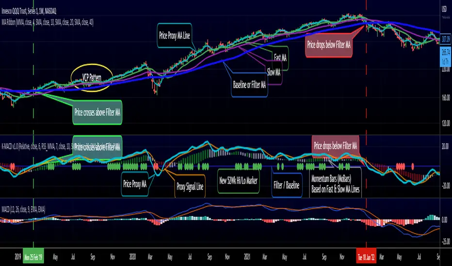
RedK K-MACD : a MACD with some more musclesMoving Averages are probably the most commonly used analysis tools, and MACD is possibly the first charting indicator a trader gets to learn about.
MACD Basic concept
----------------------------
Without repeating all the tons of documentation about what MACD does, let's quickly re-visit the MACD concept from a 10-mile altitude (note we're keen on simplifying here rather than being technically accurate - so please forgive the use of any "common lingos")
- MACD goal is to represent the distance between 2 Moving Averages (MAs) - one fast and one slow, relatively - as an unrestricted zero-based oscillator.
- The value of the main MACD line is the distance, or the displacement between the 2 MA's
- usually a signal line is used (which is another MA of that distance value) to enable better visualization of the change (and rate of change, since this is all depicted on a time axis) of that displacement - this represents price momentum (price movement in the recent period versus movements for a relatively longer period).
- the difference between the main MACD line and its signal is then represented as a histogram above and below the zero line. in this case, that histogram is really redundant, since it shows a value that is already represented visually by the main line and its signal line.
How K-MACD is different
---------------------------------
K-MACD takes that simple concept of the classic MACD and expands around it - the idea is to use the same simple approach to representing price momentum while bringing in more insight to price moves in the short, medium and long terms, ability to represent more than 2 MA's and to enable better identification of tradeable patterns (like Volatility Contraction and others) - while still keeping things simple and visually clean.
K-MACD is an indicator that allows us to view how price moves against 3 moving averages: a fast / slow pair, and a "market" Filter or Baseline (very long) that will be used as a flag for Bear/Bull market mode. Many traders and trading literature use the 200 day (40 week) SMA as that key filter
so in total, there are 4 MA lines in K-MACD (excluding the "orange" signal line):
* Price Proxy: Which is a very fast moving average that will represent the price itself - let's use a WMA(3) or something close to that here - there will be a signal line to enable better visualization of this similar to a classic MACD - that's the orange line
* Fast & Slow MA's : Use whatever represents the "medium term" momentum for your trading - Some traders use 20 and 50, others use 10 and 20 .. if on your price chart, you keep using a pair of MA's for this, use the same settings in K-MACD - these will be represented by the 3-color Momentum Bars that fluctuate above and below the baseline
* Filter/Baseline MA: Should be your long (Bullish/Bearish Mode) MA. so 100 or 200 or any other value you consider your market to be bearish below and bullish above. on K-MACD this is actually the blue zero line - everything else is "relative" to it
Review the sample chart which explains various elements and the "price chart" setup that K-MACD represents. With K-MACD you can clean up your chart from those various Moving Averages - or use a different set than the ones you already have K-MACD represent - or other indicators (like ATR channels..etc)
Other "muscles" in the K-MACD
---------------------------------------------
- Relative vs Classic Calculation Mode
A key issue with the classic MACD is that the displacement between the 2 moving averages is represented as "absolute or direct" values - as the price of the underlying increases with time, you can't really use these values to make useful comparison between the past and now (see below example) - also you can't use them to compare 2 different instruments.
- The "Relative" calculation option in K-MACD addresses that issue by relating all "distances" to the Baseline MA as percentage (above or below) - you can see this clear when you look at the above chart the far left versus the far right and compare K-MACD with the classic MACD - the Classic option is still available
- More MA "type" options for all MA lines: choose between SMA, EMA, WMA, and RSS_WMA (which i use a lot in my trading and is my default for the Price Proxy)
- More Alerts: a total or 9 alerts (in 3 groups) are available with K-MACD (Momentum above or below baseline, Price Proxy crossing signal line, and Price Proxy crossing baseline)
- New 52 week High / Low markers: These will show as Green/red circles on the zero line in K-MACD. this will only work for 1D timeframe and above, i'm just using a simple approach and would like to keep it that way.
- i know i added some more features not covered above :) -- if you have questions about any of the settings, feel free to ask below
Closing thoughts
-------------------------
K-MACD is a combination of couple of indicators i published in the past (xMACD and Mo_Bars) - so you can go back and read about them if needed - I then added improvements to accommodate ideas from swing trading literature and common practices that i plan to focus on in future. So K-MACD is really part of my own trading setup.
I assume here that most traders are familiar with what a MACD is - so kept this post short - if you thing we should expand more about the concepts covered here let me know in the comments - i can make some separate posts with examples and more details.
I hope many fellow traders find this work useful - and feel free let me know in comments below if you do.
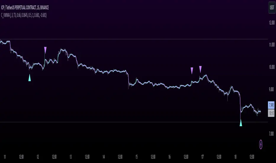
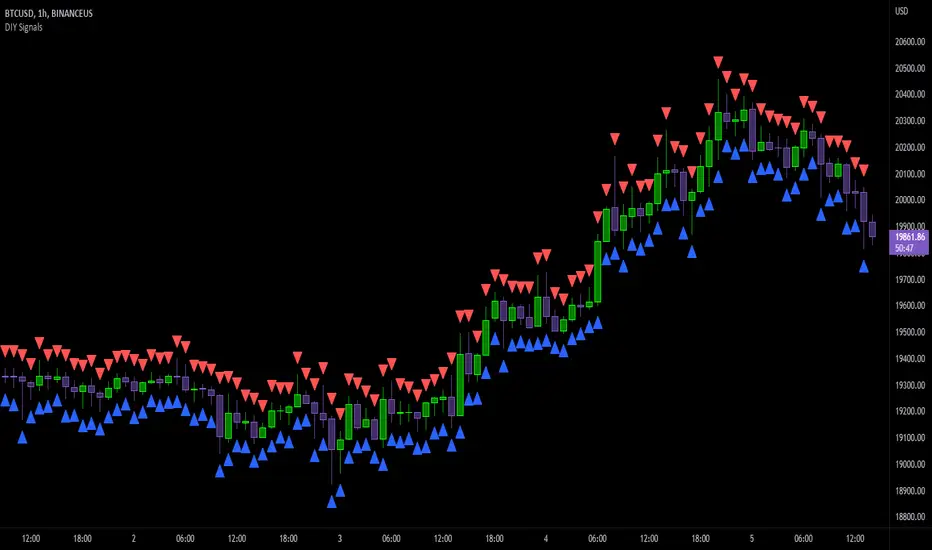
DIY Entry SignalsThis indicator allows you to set up entry signals based on your own conditions.
Note that this indicator DOES NOT give any information about exits. It is not intended to be a signal indicator that someone could blindly follow. It is intended for use in backtesting to help spot entry points more easily.
Also note that this indicator DOES NOT plot anything other than moving averages and entry signals. The other indicators referenced will need to be added on their own to be visible on the chart.
Credit to The_Caretaker for both BBWP and PMARP indicators. For more information on how those work, see their descriptions. Big thanks to him for making them open source, as well.
Instructions for use:
Signal Types:
This section allows you to choose whether you want long, short, or both types of signals.
Moving Averages:
Configure up to 4 moving averages to be plotted on the chart. Options include show/hide, color, length, and type.
RSI:
Choose the period and source used for the Relative Strength Index indicator, a very commonly used momentum oscillator.
Stochastic:
Choose the K, D, smoothing, and source for the Stochastic indicator, a very commonly used momentum oscillator.
BBWP:
Choose settings for the Bollinger Band Width Percentile indicator. This measures volatility based on Bollinger Bands and was created by The_Caretaker. The indicator is free and open source, so definitely check it out.
This section allows the user to choose the price source, basis type ( SMA , EMA , or VWMA ), length, and lookback. It also includes a threshold setting to determine the BBWP requirement used for entry signals.
PMARP:
Choose settings for the Price Moving Average Ratio & Percentile. This calculates the ratio between a source price and moving average over a lookback period. This was also created by The_Caretaker, and it is a free and open source indicator.
This section allows the user to choose price source, lookback, PMAR length, and moving average type.
DMI/ADX:
Choose settings for the Directional Movement Index and the Average Directional Index. This shows which direction the price is moving by comparing prior highs and lows and calculating a positive directional movement and a negative directional movement. The average of the positive and negative movements is used to plot the ADX line.
Long/Short Conditions:
Choose which indicators will be used to determine entry signals, as well as some options for each indicator that is included.
Note: A signal will only be plotted if ALL selected conditions are met.
Options in these sections include:
Faster moving averages above or below slower moving averages (implying a trend direction)
RSI thresholds (separate for long and short)
Stochastic thresholds (separate for long and short)
Whether K should be above or below D (implying trend direction of the Stochastic indicator)
Whether a signal should only be generated on the bar when the Stochastic first crosses the threshold.
BBWP on/off (The threshold for this is determined in the BBWP section of the settings)
PMARP thresholds (separate for long and short)
STD-Adaptive T3 [Loxx]STD-Adaptive T3 is a standard deviation adaptive T3 moving average filter. This indicator acts more like a trend overlay indicator with gradient coloring.
What is the T3 moving average?
Better Moving Averages Tim Tillson
November 1, 1998
Tim Tillson is a software project manager at Hewlett-Packard, with degrees in Mathematics and Computer Science. He has privately traded options and equities for 15 years.
Introduction
"Digital filtering includes the process of smoothing, predicting, differentiating, integrating, separation of signals, and removal of noise from a signal. Thus many people who do such things are actually using digital filters without realizing that they are; being unacquainted with the theory, they neither understand what they have done nor the possibilities of what they might have done."
This quote from R. W. Hamming applies to the vast majority of indicators in technical analysis . Moving averages, be they simple, weighted, or exponential, are lowpass filters; low frequency components in the signal pass through with little attenuation, while high frequencies are severely reduced.
"Oscillator" type indicators (such as MACD , Momentum, Relative Strength Index ) are another type of digital filter called a differentiator.
Tushar Chande has observed that many popular oscillators are highly correlated, which is sensible because they are trying to measure the rate of change of the underlying time series, i.e., are trying to be the first and second derivatives we all learned about in Calculus.
We use moving averages (lowpass filters) in technical analysis to remove the random noise from a time series, to discern the underlying trend or to determine prices at which we will take action. A perfect moving average would have two attributes:
It would be smooth, not sensitive to random noise in the underlying time series. Another way of saying this is that its derivative would not spuriously alternate between positive and negative values.
It would not lag behind the time series it is computed from. Lag, of course, produces late buy or sell signals that kill profits.
The only way one can compute a perfect moving average is to have knowledge of the future, and if we had that, we would buy one lottery ticket a week rather than trade!
Having said this, we can still improve on the conventional simple, weighted, or exponential moving averages. Here's how:
Two Interesting Moving Averages
We will examine two benchmark moving averages based on Linear Regression analysis.
In both cases, a Linear Regression line of length n is fitted to price data.
I call the first moving average ILRS, which stands for Integral of Linear Regression Slope. One simply integrates the slope of a linear regression line as it is successively fitted in a moving window of length n across the data, with the constant of integration being a simple moving average of the first n points. Put another way, the derivative of ILRS is the linear regression slope. Note that ILRS is not the same as a SMA ( simple moving average ) of length n, which is actually the midpoint of the linear regression line as it moves across the data.
We can measure the lag of moving averages with respect to a linear trend by computing how they behave when the input is a line with unit slope. Both SMA (n) and ILRS(n) have lag of n/2, but ILRS is much smoother than SMA .
Our second benchmark moving average is well known, called EPMA or End Point Moving Average. It is the endpoint of the linear regression line of length n as it is fitted across the data. EPMA hugs the data more closely than a simple or exponential moving average of the same length. The price we pay for this is that it is much noisier (less smooth) than ILRS, and it also has the annoying property that it overshoots the data when linear trends are present.
However, EPMA has a lag of 0 with respect to linear input! This makes sense because a linear regression line will fit linear input perfectly, and the endpoint of the LR line will be on the input line.
These two moving averages frame the tradeoffs that we are facing. On one extreme we have ILRS, which is very smooth and has considerable phase lag. EPMA has 0 phase lag, but is too noisy and overshoots. We would like to construct a better moving average which is as smooth as ILRS, but runs closer to where EPMA lies, without the overshoot.
A easy way to attempt this is to split the difference, i.e. use (ILRS(n)+EPMA(n))/2. This will give us a moving average (call it IE /2) which runs in between the two, has phase lag of n/4 but still inherits considerable noise from EPMA. IE /2 is inspirational, however. Can we build something that is comparable, but smoother? Figure 1 shows ILRS, EPMA, and IE /2.
Filter Techniques
Any thoughtful student of filter theory (or resolute experimenter) will have noticed that you can improve the smoothness of a filter by running it through itself multiple times, at the cost of increasing phase lag.
There is a complementary technique (called twicing by J.W. Tukey) which can be used to improve phase lag. If L stands for the operation of running data through a low pass filter, then twicing can be described by:
L' = L(time series) + L(time series - L(time series))
That is, we add a moving average of the difference between the input and the moving average to the moving average. This is algebraically equivalent to:
2L-L(L)
This is the Double Exponential Moving Average or DEMA , popularized by Patrick Mulloy in TASAC (January/February 1994).
In our taxonomy, DEMA has some phase lag (although it exponentially approaches 0) and is somewhat noisy, comparable to IE /2 indicator.
We will use these two techniques to construct our better moving average, after we explore the first one a little more closely.
Fixing Overshoot
An n-day EMA has smoothing constant alpha=2/(n+1) and a lag of (n-1)/2.
Thus EMA (3) has lag 1, and EMA (11) has lag 5. Figure 2 shows that, if I am willing to incur 5 days of lag, I get a smoother moving average if I run EMA (3) through itself 5 times than if I just take EMA (11) once.
This suggests that if EPMA and DEMA have 0 or low lag, why not run fast versions (eg DEMA (3)) through themselves many times to achieve a smooth result? The problem is that multiple runs though these filters increase their tendency to overshoot the data, giving an unusable result. This is because the amplitude response of DEMA and EPMA is greater than 1 at certain frequencies, giving a gain of much greater than 1 at these frequencies when run though themselves multiple times. Figure 3 shows DEMA (7) and EPMA(7) run through themselves 3 times. DEMA^3 has serious overshoot, and EPMA^3 is terrible.
The solution to the overshoot problem is to recall what we are doing with twicing:
DEMA (n) = EMA (n) + EMA (time series - EMA (n))
The second term is adding, in effect, a smooth version of the derivative to the EMA to achieve DEMA . The derivative term determines how hot the moving average's response to linear trends will be. We need to simply turn down the volume to achieve our basic building block:
EMA (n) + EMA (time series - EMA (n))*.7;
This is algebraically the same as:
EMA (n)*1.7-EMA( EMA (n))*.7;
I have chosen .7 as my volume factor, but the general formula (which I call "Generalized Dema") is:
GD (n,v) = EMA (n)*(1+v)-EMA( EMA (n))*v,
Where v ranges between 0 and 1. When v=0, GD is just an EMA , and when v=1, GD is DEMA . In between, GD is a cooler DEMA . By using a value for v less than 1 (I like .7), we cure the multiple DEMA overshoot problem, at the cost of accepting some additional phase delay. Now we can run GD through itself multiple times to define a new, smoother moving average T3 that does not overshoot the data:
T3(n) = GD ( GD ( GD (n)))
In filter theory parlance, T3 is a six-pole non-linear Kalman filter. Kalman filters are ones which use the error (in this case (time series - EMA (n)) to correct themselves. In Technical Analysis , these are called Adaptive Moving Averages; they track the time series more aggressively when it is making large moves.
Included
Bar coloring
Loxx's Expanded Source Types

Softmax Normalized T3 Histogram [Loxx]Softmax Normalized T3 Histogram is a T3 moving average that is morphed into a normalized oscillator from -1 to 1.
What is the Softmax function?
The softmax function, also known as softargmax: or normalized exponential function, converts a vector of K real numbers into a probability distribution of K possible outcomes. It is a generalization of the logistic function to multiple dimensions, and used in multinomial logistic regression. The softmax function is often used as the last activation function of a neural network to normalize the output of a network to a probability distribution over predicted output classes, based on Luce's choice axiom.
What is the T3 moving average?
Better Moving Averages Tim Tillson
November 1, 1998
Tim Tillson is a software project manager at Hewlett-Packard, with degrees in Mathematics and Computer Science. He has privately traded options and equities for 15 years.
Introduction
"Digital filtering includes the process of smoothing, predicting, differentiating, integrating, separation of signals, and removal of noise from a signal. Thus many people who do such things are actually using digital filters without realizing that they are; being unacquainted with the theory, they neither understand what they have done nor the possibilities of what they might have done."
This quote from R. W. Hamming applies to the vast majority of indicators in technical analysis . Moving averages, be they simple, weighted, or exponential, are lowpass filters; low frequency components in the signal pass through with little attenuation, while high frequencies are severely reduced.
"Oscillator" type indicators (such as MACD , Momentum, Relative Strength Index ) are another type of digital filter called a differentiator.
Tushar Chande has observed that many popular oscillators are highly correlated, which is sensible because they are trying to measure the rate of change of the underlying time series, i.e., are trying to be the first and second derivatives we all learned about in Calculus.
We use moving averages (lowpass filters) in technical analysis to remove the random noise from a time series, to discern the underlying trend or to determine prices at which we will take action. A perfect moving average would have two attributes:
It would be smooth, not sensitive to random noise in the underlying time series. Another way of saying this is that its derivative would not spuriously alternate between positive and negative values.
It would not lag behind the time series it is computed from. Lag, of course, produces late buy or sell signals that kill profits.
The only way one can compute a perfect moving average is to have knowledge of the future, and if we had that, we would buy one lottery ticket a week rather than trade!
Having said this, we can still improve on the conventional simple, weighted, or exponential moving averages. Here's how:
Two Interesting Moving Averages
We will examine two benchmark moving averages based on Linear Regression analysis.
In both cases, a Linear Regression line of length n is fitted to price data.
I call the first moving average ILRS, which stands for Integral of Linear Regression Slope. One simply integrates the slope of a linear regression line as it is successively fitted in a moving window of length n across the data, with the constant of integration being a simple moving average of the first n points. Put another way, the derivative of ILRS is the linear regression slope. Note that ILRS is not the same as a SMA ( simple moving average ) of length n, which is actually the midpoint of the linear regression line as it moves across the data.
We can measure the lag of moving averages with respect to a linear trend by computing how they behave when the input is a line with unit slope. Both SMA (n) and ILRS(n) have lag of n/2, but ILRS is much smoother than SMA .
Our second benchmark moving average is well known, called EPMA or End Point Moving Average. It is the endpoint of the linear regression line of length n as it is fitted across the data. EPMA hugs the data more closely than a simple or exponential moving average of the same length. The price we pay for this is that it is much noisier (less smooth) than ILRS, and it also has the annoying property that it overshoots the data when linear trends are present.
However, EPMA has a lag of 0 with respect to linear input! This makes sense because a linear regression line will fit linear input perfectly, and the endpoint of the LR line will be on the input line.
These two moving averages frame the tradeoffs that we are facing. On one extreme we have ILRS, which is very smooth and has considerable phase lag. EPMA has 0 phase lag, but is too noisy and overshoots. We would like to construct a better moving average which is as smooth as ILRS, but runs closer to where EPMA lies, without the overshoot.
A easy way to attempt this is to split the difference, i.e. use (ILRS(n)+EPMA(n))/2. This will give us a moving average (call it IE /2) which runs in between the two, has phase lag of n/4 but still inherits considerable noise from EPMA. IE /2 is inspirational, however. Can we build something that is comparable, but smoother? Figure 1 shows ILRS, EPMA, and IE /2.
Filter Techniques
Any thoughtful student of filter theory (or resolute experimenter) will have noticed that you can improve the smoothness of a filter by running it through itself multiple times, at the cost of increasing phase lag.
There is a complementary technique (called twicing by J.W. Tukey) which can be used to improve phase lag. If L stands for the operation of running data through a low pass filter, then twicing can be described by:
L' = L(time series) + L(time series - L(time series))
That is, we add a moving average of the difference between the input and the moving average to the moving average. This is algebraically equivalent to:
2L-L(L)
This is the Double Exponential Moving Average or DEMA , popularized by Patrick Mulloy in TASAC (January/February 1994).
In our taxonomy, DEMA has some phase lag (although it exponentially approaches 0) and is somewhat noisy, comparable to IE /2 indicator.
We will use these two techniques to construct our better moving average, after we explore the first one a little more closely.
Fixing Overshoot
An n-day EMA has smoothing constant alpha=2/(n+1) and a lag of (n-1)/2.
Thus EMA (3) has lag 1, and EMA (11) has lag 5. Figure 2 shows that, if I am willing to incur 5 days of lag, I get a smoother moving average if I run EMA (3) through itself 5 times than if I just take EMA (11) once.
This suggests that if EPMA and DEMA have 0 or low lag, why not run fast versions (eg DEMA (3)) through themselves many times to achieve a smooth result? The problem is that multiple runs though these filters increase their tendency to overshoot the data, giving an unusable result. This is because the amplitude response of DEMA and EPMA is greater than 1 at certain frequencies, giving a gain of much greater than 1 at these frequencies when run though themselves multiple times. Figure 3 shows DEMA (7) and EPMA(7) run through themselves 3 times. DEMA^3 has serious overshoot, and EPMA^3 is terrible.
The solution to the overshoot problem is to recall what we are doing with twicing:
DEMA (n) = EMA (n) + EMA (time series - EMA (n))
The second term is adding, in effect, a smooth version of the derivative to the EMA to achieve DEMA . The derivative term determines how hot the moving average's response to linear trends will be. We need to simply turn down the volume to achieve our basic building block:
EMA (n) + EMA (time series - EMA (n))*.7;
This is algebraically the same as:
EMA (n)*1.7-EMA( EMA (n))*.7;
I have chosen .7 as my volume factor, but the general formula (which I call "Generalized Dema") is:
GD (n,v) = EMA (n)*(1+v)-EMA( EMA (n))*v,
Where v ranges between 0 and 1. When v=0, GD is just an EMA , and when v=1, GD is DEMA . In between, GD is a cooler DEMA . By using a value for v less than 1 (I like .7), we cure the multiple DEMA overshoot problem, at the cost of accepting some additional phase delay. Now we can run GD through itself multiple times to define a new, smoother moving average T3 that does not overshoot the data:
T3(n) = GD ( GD ( GD (n)))
In filter theory parlance, T3 is a six-pole non-linear Kalman filter. Kalman filters are ones which use the error (in this case (time series - EMA (n)) to correct themselves. In Technical Analysis , these are called Adaptive Moving Averages; they track the time series more aggressively when it is making large moves.
Included:
Bar coloring
Signals
Alerts
Loxx's Expanded Source Types
T3 Velocity Candles [Loxx]T3 Velocity Candles is a candle coloring overlay that calculates its gradient coloring using T3 velocity.
What is the T3 moving average?
Better Moving Averages Tim Tillson
November 1, 1998
Tim Tillson is a software project manager at Hewlett-Packard, with degrees in Mathematics and Computer Science. He has privately traded options and equities for 15 years.
Introduction
"Digital filtering includes the process of smoothing, predicting, differentiating, integrating, separation of signals, and removal of noise from a signal. Thus many people who do such things are actually using digital filters without realizing that they are; being unacquainted with the theory, they neither understand what they have done nor the possibilities of what they might have done."
This quote from R. W. Hamming applies to the vast majority of indicators in technical analysis . Moving averages, be they simple, weighted, or exponential, are lowpass filters; low frequency components in the signal pass through with little attenuation, while high frequencies are severely reduced.
"Oscillator" type indicators (such as MACD , Momentum, Relative Strength Index ) are another type of digital filter called a differentiator.
Tushar Chande has observed that many popular oscillators are highly correlated, which is sensible because they are trying to measure the rate of change of the underlying time series, i.e., are trying to be the first and second derivatives we all learned about in Calculus.
We use moving averages (lowpass filters) in technical analysis to remove the random noise from a time series, to discern the underlying trend or to determine prices at which we will take action. A perfect moving average would have two attributes:
It would be smooth, not sensitive to random noise in the underlying time series. Another way of saying this is that its derivative would not spuriously alternate between positive and negative values.
It would not lag behind the time series it is computed from. Lag, of course, produces late buy or sell signals that kill profits.
The only way one can compute a perfect moving average is to have knowledge of the future, and if we had that, we would buy one lottery ticket a week rather than trade!
Having said this, we can still improve on the conventional simple, weighted, or exponential moving averages. Here's how:
Two Interesting Moving Averages
We will examine two benchmark moving averages based on Linear Regression analysis.
In both cases, a Linear Regression line of length n is fitted to price data.
I call the first moving average ILRS, which stands for Integral of Linear Regression Slope. One simply integrates the slope of a linear regression line as it is successively fitted in a moving window of length n across the data, with the constant of integration being a simple moving average of the first n points. Put another way, the derivative of ILRS is the linear regression slope. Note that ILRS is not the same as a SMA ( simple moving average ) of length n, which is actually the midpoint of the linear regression line as it moves across the data.
We can measure the lag of moving averages with respect to a linear trend by computing how they behave when the input is a line with unit slope. Both SMA (n) and ILRS(n) have lag of n/2, but ILRS is much smoother than SMA .
Our second benchmark moving average is well known, called EPMA or End Point Moving Average. It is the endpoint of the linear regression line of length n as it is fitted across the data. EPMA hugs the data more closely than a simple or exponential moving average of the same length. The price we pay for this is that it is much noisier (less smooth) than ILRS, and it also has the annoying property that it overshoots the data when linear trends are present.
However, EPMA has a lag of 0 with respect to linear input! This makes sense because a linear regression line will fit linear input perfectly, and the endpoint of the LR line will be on the input line.
These two moving averages frame the tradeoffs that we are facing. On one extreme we have ILRS, which is very smooth and has considerable phase lag. EPMA has 0 phase lag, but is too noisy and overshoots. We would like to construct a better moving average which is as smooth as ILRS, but runs closer to where EPMA lies, without the overshoot.
A easy way to attempt this is to split the difference, i.e. use (ILRS(n)+EPMA(n))/2. This will give us a moving average (call it IE /2) which runs in between the two, has phase lag of n/4 but still inherits considerable noise from EPMA. IE /2 is inspirational, however. Can we build something that is comparable, but smoother? Figure 1 shows ILRS, EPMA, and IE /2.
Filter Techniques
Any thoughtful student of filter theory (or resolute experimenter) will have noticed that you can improve the smoothness of a filter by running it through itself multiple times, at the cost of increasing phase lag.
There is a complementary technique (called twicing by J.W. Tukey) which can be used to improve phase lag. If L stands for the operation of running data through a low pass filter, then twicing can be described by:
L' = L(time series) + L(time series - L(time series))
That is, we add a moving average of the difference between the input and the moving average to the moving average. This is algebraically equivalent to:
2L-L(L)
This is the Double Exponential Moving Average or DEMA , popularized by Patrick Mulloy in TASAC (January/February 1994).
In our taxonomy, DEMA has some phase lag (although it exponentially approaches 0) and is somewhat noisy, comparable to IE /2 indicator.
We will use these two techniques to construct our better moving average, after we explore the first one a little more closely.
Fixing Overshoot
An n-day EMA has smoothing constant alpha=2/(n+1) and a lag of (n-1)/2.
Thus EMA (3) has lag 1, and EMA (11) has lag 5. Figure 2 shows that, if I am willing to incur 5 days of lag, I get a smoother moving average if I run EMA (3) through itself 5 times than if I just take EMA (11) once.
This suggests that if EPMA and DEMA have 0 or low lag, why not run fast versions (eg DEMA (3)) through themselves many times to achieve a smooth result? The problem is that multiple runs though these filters increase their tendency to overshoot the data, giving an unusable result. This is because the amplitude response of DEMA and EPMA is greater than 1 at certain frequencies, giving a gain of much greater than 1 at these frequencies when run though themselves multiple times. Figure 3 shows DEMA (7) and EPMA(7) run through themselves 3 times. DEMA^3 has serious overshoot, and EPMA^3 is terrible.
The solution to the overshoot problem is to recall what we are doing with twicing:
DEMA (n) = EMA (n) + EMA (time series - EMA (n))
The second term is adding, in effect, a smooth version of the derivative to the EMA to achieve DEMA . The derivative term determines how hot the moving average's response to linear trends will be. We need to simply turn down the volume to achieve our basic building block:
EMA (n) + EMA (time series - EMA (n))*.7;
This is algebraically the same as:
EMA (n)*1.7-EMA( EMA (n))*.7;
I have chosen .7 as my volume factor, but the general formula (which I call "Generalized Dema") is:
GD (n,v) = EMA (n)*(1+v)-EMA( EMA (n))*v,
Where v ranges between 0 and 1. When v=0, GD is just an EMA , and when v=1, GD is DEMA . In between, GD is a cooler DEMA . By using a value for v less than 1 (I like .7), we cure the multiple DEMA overshoot problem, at the cost of accepting some additional phase delay. Now we can run GD through itself multiple times to define a new, smoother moving average T3 that does not overshoot the data:
T3(n) = GD ( GD ( GD (n)))
In filter theory parlance, T3 is a six-pole non-linear Kalman filter. Kalman filters are ones which use the error (in this case (time series - EMA (n)) to correct themselves. In Technical Analysis , these are called Adaptive Moving Averages; they track the time series more aggressively when it is making large moves.

T3 Striped [Loxx]Theory:
Although T3 is widely used, some of the details on how it is calculated are less known. T3 has, internally, 6 "levels" or "steps" that it uses for its calculation.
This version:
Instead of showing the final T3 value, this indicator shows those intermediate steps. This shows the "building steps" of T3 and can be used for trend assessment as well as for possible support / resistance values.
What is the T3 moving average?
Better Moving Averages Tim Tillson
November 1, 1998
Tim Tillson is a software project manager at Hewlett-Packard, with degrees in Mathematics and Computer Science. He has privately traded options and equities for 15 years.
Introduction
"Digital filtering includes the process of smoothing, predicting, differentiating, integrating, separation of signals, and removal of noise from a signal. Thus many people who do such things are actually using digital filters without realizing that they are; being unacquainted with the theory, they neither understand what they have done nor the possibilities of what they might have done."
This quote from R. W. Hamming applies to the vast majority of indicators in technical analysis . Moving averages, be they simple, weighted, or exponential, are lowpass filters; low frequency components in the signal pass through with little attenuation, while high frequencies are severely reduced.
"Oscillator" type indicators (such as MACD , Momentum, Relative Strength Index ) are another type of digital filter called a differentiator.
Tushar Chande has observed that many popular oscillators are highly correlated, which is sensible because they are trying to measure the rate of change of the underlying time series, i.e., are trying to be the first and second derivatives we all learned about in Calculus.
We use moving averages (lowpass filters) in technical analysis to remove the random noise from a time series, to discern the underlying trend or to determine prices at which we will take action. A perfect moving average would have two attributes:
It would be smooth, not sensitive to random noise in the underlying time series. Another way of saying this is that its derivative would not spuriously alternate between positive and negative values.
It would not lag behind the time series it is computed from. Lag, of course, produces late buy or sell signals that kill profits.
The only way one can compute a perfect moving average is to have knowledge of the future, and if we had that, we would buy one lottery ticket a week rather than trade!
Having said this, we can still improve on the conventional simple, weighted, or exponential moving averages. Here's how:
Two Interesting Moving Averages
We will examine two benchmark moving averages based on Linear Regression analysis.
In both cases, a Linear Regression line of length n is fitted to price data.
I call the first moving average ILRS, which stands for Integral of Linear Regression Slope. One simply integrates the slope of a linear regression line as it is successively fitted in a moving window of length n across the data, with the constant of integration being a simple moving average of the first n points. Put another way, the derivative of ILRS is the linear regression slope. Note that ILRS is not the same as a SMA ( simple moving average ) of length n, which is actually the midpoint of the linear regression line as it moves across the data.
We can measure the lag of moving averages with respect to a linear trend by computing how they behave when the input is a line with unit slope. Both SMA (n) and ILRS(n) have lag of n/2, but ILRS is much smoother than SMA .
Our second benchmark moving average is well known, called EPMA or End Point Moving Average. It is the endpoint of the linear regression line of length n as it is fitted across the data. EPMA hugs the data more closely than a simple or exponential moving average of the same length. The price we pay for this is that it is much noisier (less smooth) than ILRS, and it also has the annoying property that it overshoots the data when linear trends are present.
However, EPMA has a lag of 0 with respect to linear input! This makes sense because a linear regression line will fit linear input perfectly, and the endpoint of the LR line will be on the input line.
These two moving averages frame the tradeoffs that we are facing. On one extreme we have ILRS, which is very smooth and has considerable phase lag. EPMA has 0 phase lag, but is too noisy and overshoots. We would like to construct a better moving average which is as smooth as ILRS, but runs closer to where EPMA lies, without the overshoot.
A easy way to attempt this is to split the difference, i.e. use (ILRS(n)+EPMA(n))/2. This will give us a moving average (call it IE /2) which runs in between the two, has phase lag of n/4 but still inherits considerable noise from EPMA. IE /2 is inspirational, however. Can we build something that is comparable, but smoother? Figure 1 shows ILRS, EPMA, and IE /2.
Filter Techniques
Any thoughtful student of filter theory (or resolute experimenter) will have noticed that you can improve the smoothness of a filter by running it through itself multiple times, at the cost of increasing phase lag.
There is a complementary technique (called twicing by J.W. Tukey) which can be used to improve phase lag. If L stands for the operation of running data through a low pass filter, then twicing can be described by:
L' = L(time series) + L(time series - L(time series))
That is, we add a moving average of the difference between the input and the moving average to the moving average. This is algebraically equivalent to:
2L-L(L)
This is the Double Exponential Moving Average or DEMA , popularized by Patrick Mulloy in TASAC (January/February 1994).
In our taxonomy, DEMA has some phase lag (although it exponentially approaches 0) and is somewhat noisy, comparable to IE /2 indicator.
We will use these two techniques to construct our better moving average, after we explore the first one a little more closely.
Fixing Overshoot
An n-day EMA has smoothing constant alpha=2/(n+1) and a lag of (n-1)/2.
Thus EMA (3) has lag 1, and EMA (11) has lag 5. Figure 2 shows that, if I am willing to incur 5 days of lag, I get a smoother moving average if I run EMA (3) through itself 5 times than if I just take EMA (11) once.
This suggests that if EPMA and DEMA have 0 or low lag, why not run fast versions (eg DEMA (3)) through themselves many times to achieve a smooth result? The problem is that multiple runs though these filters increase their tendency to overshoot the data, giving an unusable result. This is because the amplitude response of DEMA and EPMA is greater than 1 at certain frequencies, giving a gain of much greater than 1 at these frequencies when run though themselves multiple times. Figure 3 shows DEMA (7) and EPMA(7) run through themselves 3 times. DEMA^3 has serious overshoot, and EPMA^3 is terrible.
The solution to the overshoot problem is to recall what we are doing with twicing:
DEMA (n) = EMA (n) + EMA (time series - EMA (n))
The second term is adding, in effect, a smooth version of the derivative to the EMA to achieve DEMA . The derivative term determines how hot the moving average's response to linear trends will be. We need to simply turn down the volume to achieve our basic building block:
EMA (n) + EMA (time series - EMA (n))*.7;
This is algebraically the same as:
EMA (n)*1.7-EMA( EMA (n))*.7;
I have chosen .7 as my volume factor, but the general formula (which I call "Generalized Dema") is:
GD (n,v) = EMA (n)*(1+v)-EMA( EMA (n))*v,
Where v ranges between 0 and 1. When v=0, GD is just an EMA , and when v=1, GD is DEMA . In between, GD is a cooler DEMA . By using a value for v less than 1 (I like .7), we cure the multiple DEMA overshoot problem, at the cost of accepting some additional phase delay. Now we can run GD through itself multiple times to define a new, smoother moving average T3 that does not overshoot the data:
T3(n) = GD ( GD ( GD (n)))
In filter theory parlance, T3 is a six-pole non-linear Kalman filter. Kalman filters are ones which use the error (in this case (time series - EMA (n)) to correct themselves. In Technical Analysis , these are called Adaptive Moving Averages; they track the time series more aggressively when it is making large moves.
Included
Alerts
Signals
Bar coloring
Loxx's Expanded Source Types
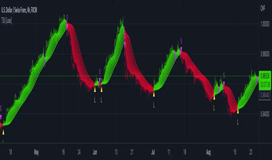
R-squared Adaptive T3 Ribbon Filled Simple [Loxx]R-squared Adaptive T3 Ribbon Filled Simple is a T3 ribbons indicator that uses a special implementation of T3 that is R-squared adaptive.
What is the T3 moving average?
Better Moving Averages Tim Tillson
November 1, 1998
Tim Tillson is a software project manager at Hewlett-Packard, with degrees in Mathematics and Computer Science. He has privately traded options and equities for 15 years.
Introduction
"Digital filtering includes the process of smoothing, predicting, differentiating, integrating, separation of signals, and removal of noise from a signal. Thus many people who do such things are actually using digital filters without realizing that they are; being unacquainted with the theory, they neither understand what they have done nor the possibilities of what they might have done."
This quote from R. W. Hamming applies to the vast majority of indicators in technical analysis . Moving averages, be they simple, weighted, or exponential, are lowpass filters; low frequency components in the signal pass through with little attenuation, while high frequencies are severely reduced.
"Oscillator" type indicators (such as MACD , Momentum, Relative Strength Index ) are another type of digital filter called a differentiator.
Tushar Chande has observed that many popular oscillators are highly correlated, which is sensible because they are trying to measure the rate of change of the underlying time series, i.e., are trying to be the first and second derivatives we all learned about in Calculus.
We use moving averages (lowpass filters) in technical analysis to remove the random noise from a time series, to discern the underlying trend or to determine prices at which we will take action. A perfect moving average would have two attributes:
It would be smooth, not sensitive to random noise in the underlying time series. Another way of saying this is that its derivative would not spuriously alternate between positive and negative values.
It would not lag behind the time series it is computed from. Lag, of course, produces late buy or sell signals that kill profits.
The only way one can compute a perfect moving average is to have knowledge of the future, and if we had that, we would buy one lottery ticket a week rather than trade!
Having said this, we can still improve on the conventional simple, weighted, or exponential moving averages. Here's how:
Two Interesting Moving Averages
We will examine two benchmark moving averages based on Linear Regression analysis.
In both cases, a Linear Regression line of length n is fitted to price data.
I call the first moving average ILRS, which stands for Integral of Linear Regression Slope. One simply integrates the slope of a linear regression line as it is successively fitted in a moving window of length n across the data, with the constant of integration being a simple moving average of the first n points. Put another way, the derivative of ILRS is the linear regression slope. Note that ILRS is not the same as a SMA ( simple moving average ) of length n, which is actually the midpoint of the linear regression line as it moves across the data.
We can measure the lag of moving averages with respect to a linear trend by computing how they behave when the input is a line with unit slope. Both SMA (n) and ILRS(n) have lag of n/2, but ILRS is much smoother than SMA .
Our second benchmark moving average is well known, called EPMA or End Point Moving Average. It is the endpoint of the linear regression line of length n as it is fitted across the data. EPMA hugs the data more closely than a simple or exponential moving average of the same length. The price we pay for this is that it is much noisier (less smooth) than ILRS, and it also has the annoying property that it overshoots the data when linear trends are present.
However, EPMA has a lag of 0 with respect to linear input! This makes sense because a linear regression line will fit linear input perfectly, and the endpoint of the LR line will be on the input line.
These two moving averages frame the tradeoffs that we are facing. On one extreme we have ILRS, which is very smooth and has considerable phase lag. EPMA has 0 phase lag, but is too noisy and overshoots. We would like to construct a better moving average which is as smooth as ILRS, but runs closer to where EPMA lies, without the overshoot.
A easy way to attempt this is to split the difference, i.e. use (ILRS(n)+EPMA(n))/2. This will give us a moving average (call it IE /2) which runs in between the two, has phase lag of n/4 but still inherits considerable noise from EPMA. IE /2 is inspirational, however. Can we build something that is comparable, but smoother? Figure 1 shows ILRS, EPMA, and IE /2.
Filter Techniques
Any thoughtful student of filter theory (or resolute experimenter) will have noticed that you can improve the smoothness of a filter by running it through itself multiple times, at the cost of increasing phase lag.
There is a complementary technique (called twicing by J.W. Tukey) which can be used to improve phase lag. If L stands for the operation of running data through a low pass filter, then twicing can be described by:
L' = L(time series) + L(time series - L(time series))
That is, we add a moving average of the difference between the input and the moving average to the moving average. This is algebraically equivalent to:
2L-L(L)
This is the Double Exponential Moving Average or DEMA , popularized by Patrick Mulloy in TASAC (January/February 1994).
In our taxonomy, DEMA has some phase lag (although it exponentially approaches 0) and is somewhat noisy, comparable to IE /2 indicator.
We will use these two techniques to construct our better moving average, after we explore the first one a little more closely.
Fixing Overshoot
An n-day EMA has smoothing constant alpha=2/(n+1) and a lag of (n-1)/2.
Thus EMA (3) has lag 1, and EMA (11) has lag 5. Figure 2 shows that, if I am willing to incur 5 days of lag, I get a smoother moving average if I run EMA (3) through itself 5 times than if I just take EMA (11) once.
This suggests that if EPMA and DEMA have 0 or low lag, why not run fast versions (eg DEMA (3)) through themselves many times to achieve a smooth result? The problem is that multiple runs though these filters increase their tendency to overshoot the data, giving an unusable result. This is because the amplitude response of DEMA and EPMA is greater than 1 at certain frequencies, giving a gain of much greater than 1 at these frequencies when run though themselves multiple times. Figure 3 shows DEMA (7) and EPMA(7) run through themselves 3 times. DEMA^3 has serious overshoot, and EPMA^3 is terrible.
The solution to the overshoot problem is to recall what we are doing with twicing:
DEMA (n) = EMA (n) + EMA (time series - EMA (n))
The second term is adding, in effect, a smooth version of the derivative to the EMA to achieve DEMA . The derivative term determines how hot the moving average's response to linear trends will be. We need to simply turn down the volume to achieve our basic building block:
EMA (n) + EMA (time series - EMA (n))*.7;
This is algebraically the same as:
EMA (n)*1.7-EMA( EMA (n))*.7;
I have chosen .7 as my volume factor, but the general formula (which I call "Generalized Dema") is:
GD (n,v) = EMA (n)*(1+v)-EMA( EMA (n))*v,
Where v ranges between 0 and 1. When v=0, GD is just an EMA , and when v=1, GD is DEMA . In between, GD is a cooler DEMA . By using a value for v less than 1 (I like .7), we cure the multiple DEMA overshoot problem, at the cost of accepting some additional phase delay. Now we can run GD through itself multiple times to define a new, smoother moving average T3 that does not overshoot the data:
T3(n) = GD ( GD ( GD (n)))
In filter theory parlance, T3 is a six-pole non-linear Kalman filter. Kalman filters are ones which use the error (in this case (time series - EMA (n)) to correct themselves. In Technical Analysis , these are called Adaptive Moving Averages; they track the time series more aggressively when it is making large moves.
What is R-squared Adaptive?
One tool available in forecasting the trendiness of the breakout is the coefficient of determination ( R-squared ), a statistical measurement.
The R-squared indicates linear strength between the security's price (the Y - axis) and time (the X - axis). The R-squared is the percentage of squared error that the linear regression can eliminate if it were used as the predictor instead of the mean value. If the R-squared were 0.99, then the linear regression would eliminate 99% of the error for prediction versus predicting closing prices using a simple moving average .
R-squared is used here to derive a T3 factor used to modify price before passing price through a six-pole non-linear Kalman filter.
Included:
Alerts
Signals
Loxx's Expanded Source Types
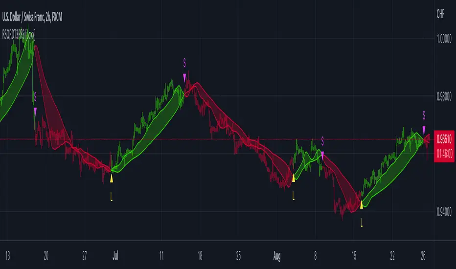
T3 Slope Variation [Loxx]T3 Slope Variation is an indicator that uses T3 moving average to calculate a slope that is then weighted to derive a signal.
The center line
The center line changes color depending on the value of the:
Slope
Signal line
Threshold
If the value is above a signal line (it is not visible on the chart) and the threshold is greater than the required, then the main trend becomes up. And reversed for the trend down.
Colors and style of the histogram
The colors and style of the histogram will be drawn if the value is at the right side, if the above described trend "agrees" with the value (above is green or below zero is red) and if the High is higher than the previous High or Low is lower than the previous low, then the according type of histogram is drawn.
What is the T3 moving average?
Better Moving Averages Tim Tillson
November 1, 1998
Tim Tillson is a software project manager at Hewlett-Packard, with degrees in Mathematics and Computer Science. He has privately traded options and equities for 15 years.
Introduction
"Digital filtering includes the process of smoothing, predicting, differentiating, integrating, separation of signals, and removal of noise from a signal. Thus many people who do such things are actually using digital filters without realizing that they are; being unacquainted with the theory, they neither understand what they have done nor the possibilities of what they might have done."
This quote from R. W. Hamming applies to the vast majority of indicators in technical analysis . Moving averages, be they simple, weighted, or exponential, are lowpass filters; low frequency components in the signal pass through with little attenuation, while high frequencies are severely reduced.
"Oscillator" type indicators (such as MACD , Momentum, Relative Strength Index ) are another type of digital filter called a differentiator.
Tushar Chande has observed that many popular oscillators are highly correlated, which is sensible because they are trying to measure the rate of change of the underlying time series, i.e., are trying to be the first and second derivatives we all learned about in Calculus.
We use moving averages (lowpass filters) in technical analysis to remove the random noise from a time series, to discern the underlying trend or to determine prices at which we will take action. A perfect moving average would have two attributes:
It would be smooth, not sensitive to random noise in the underlying time series. Another way of saying this is that its derivative would not spuriously alternate between positive and negative values.
It would not lag behind the time series it is computed from. Lag, of course, produces late buy or sell signals that kill profits.
The only way one can compute a perfect moving average is to have knowledge of the future, and if we had that, we would buy one lottery ticket a week rather than trade!
Having said this, we can still improve on the conventional simple, weighted, or exponential moving averages. Here's how:
Two Interesting Moving Averages
We will examine two benchmark moving averages based on Linear Regression analysis.
In both cases, a Linear Regression line of length n is fitted to price data.
I call the first moving average ILRS, which stands for Integral of Linear Regression Slope. One simply integrates the slope of a linear regression line as it is successively fitted in a moving window of length n across the data, with the constant of integration being a simple moving average of the first n points. Put another way, the derivative of ILRS is the linear regression slope. Note that ILRS is not the same as a SMA ( simple moving average ) of length n, which is actually the midpoint of the linear regression line as it moves across the data.
We can measure the lag of moving averages with respect to a linear trend by computing how they behave when the input is a line with unit slope. Both SMA (n) and ILRS(n) have lag of n/2, but ILRS is much smoother than SMA .
Our second benchmark moving average is well known, called EPMA or End Point Moving Average. It is the endpoint of the linear regression line of length n as it is fitted across the data. EPMA hugs the data more closely than a simple or exponential moving average of the same length. The price we pay for this is that it is much noisier (less smooth) than ILRS, and it also has the annoying property that it overshoots the data when linear trends are present.
However, EPMA has a lag of 0 with respect to linear input! This makes sense because a linear regression line will fit linear input perfectly, and the endpoint of the LR line will be on the input line.
These two moving averages frame the tradeoffs that we are facing. On one extreme we have ILRS, which is very smooth and has considerable phase lag. EPMA has 0 phase lag, but is too noisy and overshoots. We would like to construct a better moving average which is as smooth as ILRS, but runs closer to where EPMA lies, without the overshoot.
A easy way to attempt this is to split the difference, i.e. use (ILRS(n)+EPMA(n))/2. This will give us a moving average (call it IE /2) which runs in between the two, has phase lag of n/4 but still inherits considerable noise from EPMA. IE /2 is inspirational, however. Can we build something that is comparable, but smoother? Figure 1 shows ILRS, EPMA, and IE /2.
Filter Techniques
Any thoughtful student of filter theory (or resolute experimenter) will have noticed that you can improve the smoothness of a filter by running it through itself multiple times, at the cost of increasing phase lag.
There is a complementary technique (called twicing by J.W. Tukey) which can be used to improve phase lag. If L stands for the operation of running data through a low pass filter, then twicing can be described by:
L' = L(time series) + L(time series - L(time series))
That is, we add a moving average of the difference between the input and the moving average to the moving average. This is algebraically equivalent to:
2L-L(L)
This is the Double Exponential Moving Average or DEMA , popularized by Patrick Mulloy in TASAC (January/February 1994).
In our taxonomy, DEMA has some phase lag (although it exponentially approaches 0) and is somewhat noisy, comparable to IE /2 indicator.
We will use these two techniques to construct our better moving average, after we explore the first one a little more closely.
Fixing Overshoot
An n-day EMA has smoothing constant alpha=2/(n+1) and a lag of (n-1)/2.
Thus EMA (3) has lag 1, and EMA (11) has lag 5. Figure 2 shows that, if I am willing to incur 5 days of lag, I get a smoother moving average if I run EMA (3) through itself 5 times than if I just take EMA (11) once.
This suggests that if EPMA and DEMA have 0 or low lag, why not run fast versions (eg DEMA (3)) through themselves many times to achieve a smooth result? The problem is that multiple runs though these filters increase their tendency to overshoot the data, giving an unusable result. This is because the amplitude response of DEMA and EPMA is greater than 1 at certain frequencies, giving a gain of much greater than 1 at these frequencies when run though themselves multiple times. Figure 3 shows DEMA (7) and EPMA(7) run through themselves 3 times. DEMA^3 has serious overshoot, and EPMA^3 is terrible.
The solution to the overshoot problem is to recall what we are doing with twicing:
DEMA (n) = EMA (n) + EMA (time series - EMA (n))
The second term is adding, in effect, a smooth version of the derivative to the EMA to achieve DEMA . The derivative term determines how hot the moving average's response to linear trends will be. We need to simply turn down the volume to achieve our basic building block:
EMA (n) + EMA (time series - EMA (n))*.7;
This is algebraically the same as:
EMA (n)*1.7-EMA( EMA (n))*.7;
I have chosen .7 as my volume factor, but the general formula (which I call "Generalized Dema") is:
GD (n,v) = EMA (n)*(1+v)-EMA( EMA (n))*v,
Where v ranges between 0 and 1. When v=0, GD is just an EMA , and when v=1, GD is DEMA . In between, GD is a cooler DEMA . By using a value for v less than 1 (I like .7), we cure the multiple DEMA overshoot problem, at the cost of accepting some additional phase delay. Now we can run GD through itself multiple times to define a new, smoother moving average T3 that does not overshoot the data:
T3(n) = GD ( GD ( GD (n)))
In filter theory parlance, T3 is a six-pole non-linear Kalman filter. Kalman filters are ones which use the error (in this case (time series - EMA (n)) to correct themselves. In Technical Analysis , these are called Adaptive Moving Averages; they track the time series more aggressively when it is making large moves.
Included
Alets
Signals
Bar coloring
Loxx's Expanded Source Types
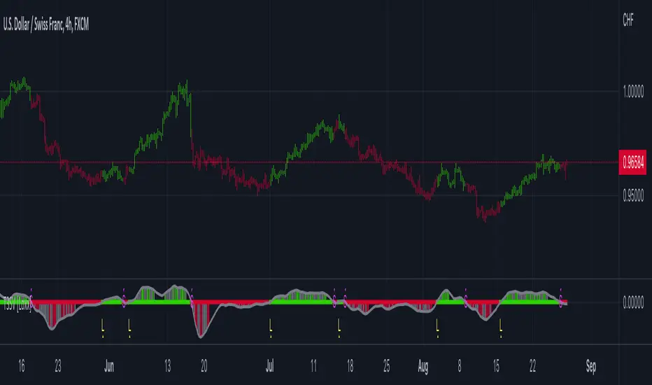
T3 Volatility Quality Index (VQI) w/ DSL & Pips Filtering [Loxx]T3 Volatility Quality Index (VQI) w/ DSL & Pips Filtering is a VQI indicator that uses T3 smoothing and discontinued signal lines to determine breakouts and breakdowns. This also allows filtering by pips.***
What is the Volatility Quality Index ( VQI )?
The idea behind the volatility quality index is to point out the difference between bad and good volatility in order to identify better trade opportunities in the market. This forex indicator works using the True Range algorithm in combination with the open, close, high and low prices.
What are DSL Discontinued Signal Line?
A lot of indicators are using signal lines in order to determine the trend (or some desired state of the indicator) easier. The idea of the signal line is easy : comparing the value to it's smoothed (slightly lagging) state, the idea of current momentum/state is made.
Discontinued signal line is inheriting that simple signal line idea and it is extending it : instead of having one signal line, more lines depending on the current value of the indicator.
"Signal" line is calculated the following way :
When a certain level is crossed into the desired direction, the EMA of that value is calculated for the desired signal line
When that level is crossed into the opposite direction, the previous "signal" line value is simply "inherited" and it becomes a kind of a level
This way it becomes a combination of signal lines and levels that are trying to combine both the good from both methods.
In simple terms, DSL uses the concept of a signal line and betters it by inheriting the previous signal line's value & makes it a level.
What is the T3 moving average?
Better Moving Averages Tim Tillson
November 1, 1998
Tim Tillson is a software project manager at Hewlett-Packard, with degrees in Mathematics and Computer Science. He has privately traded options and equities for 15 years.
Introduction
"Digital filtering includes the process of smoothing, predicting, differentiating, integrating, separation of signals, and removal of noise from a signal. Thus many people who do such things are actually using digital filters without realizing that they are; being unacquainted with the theory, they neither understand what they have done nor the possibilities of what they might have done."
This quote from R. W. Hamming applies to the vast majority of indicators in technical analysis . Moving averages, be they simple, weighted, or exponential, are lowpass filters; low frequency components in the signal pass through with little attenuation, while high frequencies are severely reduced.
"Oscillator" type indicators (such as MACD , Momentum, Relative Strength Index ) are another type of digital filter called a differentiator.
Tushar Chande has observed that many popular oscillators are highly correlated, which is sensible because they are trying to measure the rate of change of the underlying time series, i.e., are trying to be the first and second derivatives we all learned about in Calculus.
We use moving averages (lowpass filters) in technical analysis to remove the random noise from a time series, to discern the underlying trend or to determine prices at which we will take action. A perfect moving average would have two attributes:
It would be smooth, not sensitive to random noise in the underlying time series. Another way of saying this is that its derivative would not spuriously alternate between positive and negative values.
It would not lag behind the time series it is computed from. Lag, of course, produces late buy or sell signals that kill profits.
The only way one can compute a perfect moving average is to have knowledge of the future, and if we had that, we would buy one lottery ticket a week rather than trade!
Having said this, we can still improve on the conventional simple, weighted, or exponential moving averages. Here's how:
Two Interesting Moving Averages
We will examine two benchmark moving averages based on Linear Regression analysis.
In both cases, a Linear Regression line of length n is fitted to price data.
I call the first moving average ILRS, which stands for Integral of Linear Regression Slope. One simply integrates the slope of a linear regression line as it is successively fitted in a moving window of length n across the data, with the constant of integration being a simple moving average of the first n points. Put another way, the derivative of ILRS is the linear regression slope. Note that ILRS is not the same as a SMA ( simple moving average ) of length n, which is actually the midpoint of the linear regression line as it moves across the data.
We can measure the lag of moving averages with respect to a linear trend by computing how they behave when the input is a line with unit slope. Both SMA (n) and ILRS(n) have lag of n/2, but ILRS is much smoother than SMA .
Our second benchmark moving average is well known, called EPMA or End Point Moving Average. It is the endpoint of the linear regression line of length n as it is fitted across the data. EPMA hugs the data more closely than a simple or exponential moving average of the same length. The price we pay for this is that it is much noisier (less smooth) than ILRS, and it also has the annoying property that it overshoots the data when linear trends are present.
However, EPMA has a lag of 0 with respect to linear input! This makes sense because a linear regression line will fit linear input perfectly, and the endpoint of the LR line will be on the input line.
These two moving averages frame the tradeoffs that we are facing. On one extreme we have ILRS, which is very smooth and has considerable phase lag. EPMA has 0 phase lag, but is too noisy and overshoots. We would like to construct a better moving average which is as smooth as ILRS, but runs closer to where EPMA lies, without the overshoot.
A easy way to attempt this is to split the difference, i.e. use (ILRS(n)+EPMA(n))/2. This will give us a moving average (call it IE /2) which runs in between the two, has phase lag of n/4 but still inherits considerable noise from EPMA. IE /2 is inspirational, however. Can we build something that is comparable, but smoother? Figure 1 shows ILRS, EPMA, and IE /2.
Filter Techniques
Any thoughtful student of filter theory (or resolute experimenter) will have noticed that you can improve the smoothness of a filter by running it through itself multiple times, at the cost of increasing phase lag.
There is a complementary technique (called twicing by J.W. Tukey) which can be used to improve phase lag. If L stands for the operation of running data through a low pass filter, then twicing can be described by:
L' = L(time series) + L(time series - L(time series))
That is, we add a moving average of the difference between the input and the moving average to the moving average. This is algebraically equivalent to:
2L-L(L)
This is the Double Exponential Moving Average or DEMA , popularized by Patrick Mulloy in TASAC (January/February 1994).
In our taxonomy, DEMA has some phase lag (although it exponentially approaches 0) and is somewhat noisy, comparable to IE /2 indicator.
We will use these two techniques to construct our better moving average, after we explore the first one a little more closely.
Fixing Overshoot
An n-day EMA has smoothing constant alpha=2/(n+1) and a lag of (n-1)/2.
Thus EMA (3) has lag 1, and EMA (11) has lag 5. Figure 2 shows that, if I am willing to incur 5 days of lag, I get a smoother moving average if I run EMA (3) through itself 5 times than if I just take EMA (11) once.
This suggests that if EPMA and DEMA have 0 or low lag, why not run fast versions (eg DEMA (3)) through themselves many times to achieve a smooth result? The problem is that multiple runs though these filters increase their tendency to overshoot the data, giving an unusable result. This is because the amplitude response of DEMA and EPMA is greater than 1 at certain frequencies, giving a gain of much greater than 1 at these frequencies when run though themselves multiple times. Figure 3 shows DEMA (7) and EPMA(7) run through themselves 3 times. DEMA^3 has serious overshoot, and EPMA^3 is terrible.
The solution to the overshoot problem is to recall what we are doing with twicing:
DEMA (n) = EMA (n) + EMA (time series - EMA (n))
The second term is adding, in effect, a smooth version of the derivative to the EMA to achieve DEMA . The derivative term determines how hot the moving average's response to linear trends will be. We need to simply turn down the volume to achieve our basic building block:
EMA (n) + EMA (time series - EMA (n))*.7;
This is algebraically the same as:
EMA (n)*1.7-EMA( EMA (n))*.7;
I have chosen .7 as my volume factor, but the general formula (which I call "Generalized Dema") is:
GD (n,v) = EMA (n)*(1+v)-EMA( EMA (n))*v,
Where v ranges between 0 and 1. When v=0, GD is just an EMA , and when v=1, GD is DEMA . In between, GD is a cooler DEMA . By using a value for v less than 1 (I like .7), we cure the multiple DEMA overshoot problem, at the cost of accepting some additional phase delay. Now we can run GD through itself multiple times to define a new, smoother moving average T3 that does not overshoot the data:
T3(n) = GD ( GD ( GD (n)))
In filter theory parlance, T3 is a six-pole non-linear Kalman filter. Kalman filters are ones which use the error (in this case (time series - EMA (n)) to correct themselves. In Technical Analysis , these are called Adaptive Moving Averages; they track the time series more aggressively when it is making large moves.
Included
Signals
Alerts
Related indicators
Zero-line Volatility Quality Index (VQI)
Volatility Quality Index w/ Pips Filtering
Variety Moving Average Waddah Attar Explosion (WAE)
***This indicator is tuned to Forex. If you want to make it useful for other tickers, you must change the pip filtering value to match the asset. This means that for BTC, for example, you likely need to use a value of 10,000 or more for pips filter.

Gators Oscillator - Bitcoin Scalp Trader(T&M/e V3!!)Gator's Oscillator:
**For reference, all numbers, and settings displayed on the input screen are only what I HAVE FOUND to be profitable for my own strategy, Yours will differ. This is not financial advice and I am not a financial advisor. Please do your due diligence and own research before considering taking entries based on this strategy and indicator. I am not advertising investing, trading, or skills untaught, this is simply to help incorporate into your own strategy and improve your trading journey!**
INPUTS:
EV: This is an integer value set to default at 55. This value is equated to the lead value, volatility measurement, and standard deviation between averages
EV 2: This integer is used as the base value and is meant to always be GREATER THEN EV, the default is set at 163. There should be at least a 90+ integer difference between EVs for data accuracy.
EV TYPE & EV TYPE 2: This option only affects the output for the moving average histograms. (and data inserted for strategy)
Volatility Smoothing: This is the smoothness of the custom-made volatility oscillator. I have this default at 1 to show time-worthy-term (3.9%+) moves or significant trends to correspond with the standard deviation declination between EVMA and EVMA2.
Directional Length: This is the amount of data observed per candle in the bull versus bear indicator.
Take Profit: Pre-set takes profit level that is set to 4 but can be adjusted for user experience.
Style:
Base Length: Columns equated using a custom-made statistical equation derived from EV TYPE 2+EV2 to determine a range of differential in historic averages to a micro-scale.
Lead Length: Columns equated using a custom-made statistical equation derived from EV TYPE+EV to determine a range of differential in historic averages to a micro-scale.
Weighted EMA Differential: Equation expressing the differences between exponential and simple averages derived from EV+EV Type 2. Default is displaying none, but optional for use if found helpful.
Volatility: Represents volatility from multiple data sets spanning from Bollinger bands to HPV and translated through smoothing.
Bull Strength: The strength of Bulls in the current trend is derived from a DMI+RSI+MACD equation to represent where the trend lies.
Bear Strength: The strength of Bears in the current trend is derived from a DMI+RSI+MACD equation to represent where the trend lies.
(NEW) Standard Deviation between Moving Averages: Use this logarithmic indicator depicted as circles to help determine whether a move is a fake out or not. Compare the circles with the volatility line, if you see them deviating away, it is either a bull/bear trap or trend continuation is imminent until they correlate back together.
CHEAT CODE'S NOTES:
Do not use this indicator on high leverage. I have personally used this indicator for a week and faced a max of 8% drawdown, albeit painful I was on low leverage and still closed on my take profit level.
85% is not 100% do not overtrade using this indicator's entry conditions if you have made 4 consecutive profitable trades.
Mess around with the input values and let me know if you find an even BETTER hit rate, 30+ entries, and a good drawdown!!
V2 UPGRADES:
*Increased Opacity on Bull Bear Columns
*Removed the Stop Loss Input option
*Decreased EV2 to a default of 143 for accuracy
*Added additional disclaimers in the description
* Removed Bull/Bear offset values for accuracy
V3 UPGRADES:
*ADDED THE EMA DIFFERENTIAL FROM SMA STANDARD DEVIATION INDICATOR. REPRESENTED BY PURPLE BARS THAT PLOT BRIGHT AT EXTREME LEVELS (Translate this to the EMA's and SMA's are very far apart) This is a fantastic way to resolve volatility and momentum in one indicator!!
*Line Width increased for volatility
*plot's for Oversold Alma reduced to 3, also adjusted the plot shape to arrows corresponding to 'overbought/oversold values. Look for a cross-over from green/red plot to transparent for best signals.
*Histograms for bull/bear strength correspond to an increase or decrease in value
*Input screen converted into groups, with bull/bear color inline
*Converted base/lead length value's into areas with breaks. IF YOU SEE WHITE (Short/Lead Length), IT IS A SHORT TERM MOVE AND SCALPING OPPORTUNITY. IF YOU SEE BLUE(Long/Base Length) IT MEANS IT IS A MACRO MOVE, WHICH MAY LAST LONGER
-Cheat Code
BINANCE:BTCUSDT BYBIT:BTCUSDT COINBASE:BTCUSD

VHF-Adaptive T3 iTrend [Loxx]VHF-Adaptive T3 iTrend is an iTrend indicator with T3 smoothing and Vertical Horizontal Filter Adaptive period input. iTrend is used to determine where the trend starts and ends. You'll notice that the noise filter on this one is extreme. Adjust the period inputs accordingly to suit your take and your backtest requirements. This is also useful for scalping lower timeframes. Enjoy!
What is VHF Adaptive Period?
Vertical Horizontal Filter (VHF) was created by Adam White to identify trending and ranging markets. VHF measures the level of trend activity, similar to ADX DI. Vertical Horizontal Filter does not, itself, generate trading signals, but determines whether signals are taken from trend or momentum indicators. Using this trend information, one is then able to derive an average cycle length.
What is the T3 moving average?
Better Moving Averages Tim Tillson
November 1, 1998
Tim Tillson is a software project manager at Hewlett-Packard, with degrees in Mathematics and Computer Science. He has privately traded options and equities for 15 years.
Introduction
"Digital filtering includes the process of smoothing, predicting, differentiating, integrating, separation of signals, and removal of noise from a signal. Thus many people who do such things are actually using digital filters without realizing that they are; being unacquainted with the theory, they neither understand what they have done nor the possibilities of what they might have done."
This quote from R. W. Hamming applies to the vast majority of indicators in technical analysis . Moving averages, be they simple, weighted, or exponential, are lowpass filters; low frequency components in the signal pass through with little attenuation, while high frequencies are severely reduced.
"Oscillator" type indicators (such as MACD , Momentum, Relative Strength Index ) are another type of digital filter called a differentiator.
Tushar Chande has observed that many popular oscillators are highly correlated, which is sensible because they are trying to measure the rate of change of the underlying time series, i.e., are trying to be the first and second derivatives we all learned about in Calculus.
We use moving averages (lowpass filters) in technical analysis to remove the random noise from a time series, to discern the underlying trend or to determine prices at which we will take action. A perfect moving average would have two attributes:
It would be smooth, not sensitive to random noise in the underlying time series. Another way of saying this is that its derivative would not spuriously alternate between positive and negative values.
It would not lag behind the time series it is computed from. Lag, of course, produces late buy or sell signals that kill profits.
The only way one can compute a perfect moving average is to have knowledge of the future, and if we had that, we would buy one lottery ticket a week rather than trade!
Having said this, we can still improve on the conventional simple, weighted, or exponential moving averages. Here's how:
Two Interesting Moving Averages
We will examine two benchmark moving averages based on Linear Regression analysis.
In both cases, a Linear Regression line of length n is fitted to price data.
I call the first moving average ILRS, which stands for Integral of Linear Regression Slope. One simply integrates the slope of a linear regression line as it is successively fitted in a moving window of length n across the data, with the constant of integration being a simple moving average of the first n points. Put another way, the derivative of ILRS is the linear regression slope. Note that ILRS is not the same as a SMA ( simple moving average ) of length n, which is actually the midpoint of the linear regression line as it moves across the data.
We can measure the lag of moving averages with respect to a linear trend by computing how they behave when the input is a line with unit slope. Both SMA (n) and ILRS(n) have lag of n/2, but ILRS is much smoother than SMA .
Our second benchmark moving average is well known, called EPMA or End Point Moving Average. It is the endpoint of the linear regression line of length n as it is fitted across the data. EPMA hugs the data more closely than a simple or exponential moving average of the same length. The price we pay for this is that it is much noisier (less smooth) than ILRS, and it also has the annoying property that it overshoots the data when linear trends are present.
However, EPMA has a lag of 0 with respect to linear input! This makes sense because a linear regression line will fit linear input perfectly, and the endpoint of the LR line will be on the input line.
These two moving averages frame the tradeoffs that we are facing. On one extreme we have ILRS, which is very smooth and has considerable phase lag. EPMA has 0 phase lag, but is too noisy and overshoots. We would like to construct a better moving average which is as smooth as ILRS, but runs closer to where EPMA lies, without the overshoot.
A easy way to attempt this is to split the difference, i.e. use (ILRS(n)+EPMA(n))/2. This will give us a moving average (call it IE /2) which runs in between the two, has phase lag of n/4 but still inherits considerable noise from EPMA. IE /2 is inspirational, however. Can we build something that is comparable, but smoother? Figure 1 shows ILRS, EPMA, and IE /2.
Filter Techniques
Any thoughtful student of filter theory (or resolute experimenter) will have noticed that you can improve the smoothness of a filter by running it through itself multiple times, at the cost of increasing phase lag.
There is a complementary technique (called twicing by J.W. Tukey) which can be used to improve phase lag. If L stands for the operation of running data through a low pass filter, then twicing can be described by:
L' = L(time series) + L(time series - L(time series))
That is, we add a moving average of the difference between the input and the moving average to the moving average. This is algebraically equivalent to:
2L-L(L)
This is the Double Exponential Moving Average or DEMA , popularized by Patrick Mulloy in TASAC (January/February 1994).
In our taxonomy, DEMA has some phase lag (although it exponentially approaches 0) and is somewhat noisy, comparable to IE /2 indicator.
We will use these two techniques to construct our better moving average, after we explore the first one a little more closely.
Fixing Overshoot
An n-day EMA has smoothing constant alpha=2/(n+1) and a lag of (n-1)/2.
Thus EMA (3) has lag 1, and EMA (11) has lag 5. Figure 2 shows that, if I am willing to incur 5 days of lag, I get a smoother moving average if I run EMA (3) through itself 5 times than if I just take EMA (11) once.
This suggests that if EPMA and DEMA have 0 or low lag, why not run fast versions (eg DEMA (3)) through themselves many times to achieve a smooth result? The problem is that multiple runs though these filters increase their tendency to overshoot the data, giving an unusable result. This is because the amplitude response of DEMA and EPMA is greater than 1 at certain frequencies, giving a gain of much greater than 1 at these frequencies when run though themselves multiple times. Figure 3 shows DEMA (7) and EPMA(7) run through themselves 3 times. DEMA^3 has serious overshoot, and EPMA^3 is terrible.
The solution to the overshoot problem is to recall what we are doing with twicing:
DEMA (n) = EMA (n) + EMA (time series - EMA (n))
The second term is adding, in effect, a smooth version of the derivative to the EMA to achieve DEMA . The derivative term determines how hot the moving average's response to linear trends will be. We need to simply turn down the volume to achieve our basic building block:
EMA (n) + EMA (time series - EMA (n))*.7;
This is algebraically the same as:
EMA (n)*1.7-EMA( EMA (n))*.7;
I have chosen .7 as my volume factor, but the general formula (which I call "Generalized Dema") is:
GD (n,v) = EMA (n)*(1+v)-EMA( EMA (n))*v,
Where v ranges between 0 and 1. When v=0, GD is just an EMA , and when v=1, GD is DEMA . In between, GD is a cooler DEMA . By using a value for v less than 1 (I like .7), we cure the multiple DEMA overshoot problem, at the cost of accepting some additional phase delay. Now we can run GD through itself multiple times to define a new, smoother moving average T3 that does not overshoot the data:
T3(n) = GD ( GD ( GD (n)))
In filter theory parlance, T3 is a six-pole non-linear Kalman filter. Kalman filters are ones which use the error (in this case (time series - EMA (n)) to correct themselves. In Technical Analysis , these are called Adaptive Moving Averages; they track the time series more aggressively when it is making large moves.
Included
Bar coloring
Alerts
Signals
Loxx's Expanded Source Types
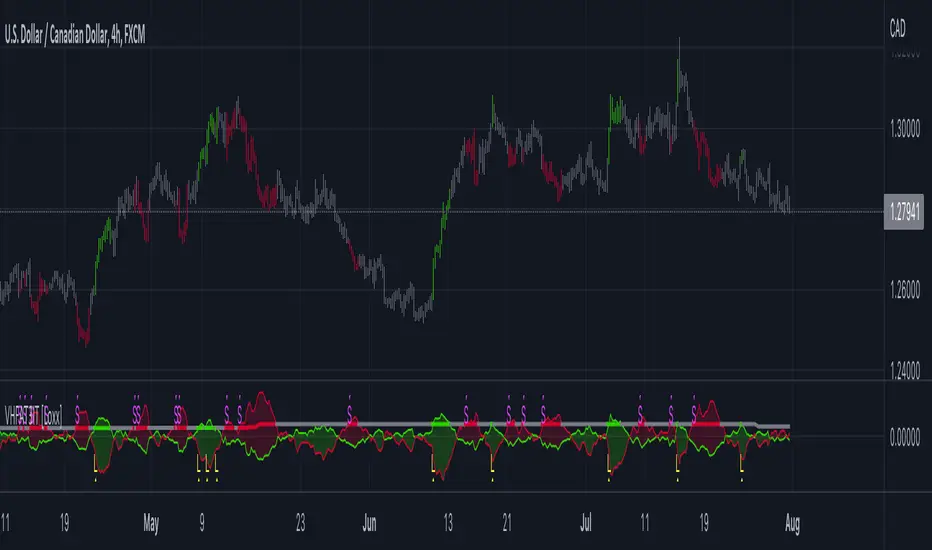
STD-Adaptive T3 Channel w/ Ehlers Swiss Army Knife Mod. [Loxx]STD-Adaptive T3 Channel w/ Ehlers Swiss Army Knife Mod. is an adaptive T3 indicator using standard deviation adaptivity and Ehlers Swiss Army Knife indicator to adjust the alpha value of the T3 calculation. This helps identify trends and reduce noise. In addition. I've included a Keltner Channel to show reversal/exhaustion zones.
What is the Swiss Army Knife Indicator?
John Ehlers explains the calculation here: www.mesasoftware.com
What is the T3 moving average?
Better Moving Averages Tim Tillson
November 1, 1998
Tim Tillson is a software project manager at Hewlett-Packard, with degrees in Mathematics and Computer Science. He has privately traded options and equities for 15 years.
Introduction
"Digital filtering includes the process of smoothing, predicting, differentiating, integrating, separation of signals, and removal of noise from a signal. Thus many people who do such things are actually using digital filters without realizing that they are; being unacquainted with the theory, they neither understand what they have done nor the possibilities of what they might have done."
This quote from R. W. Hamming applies to the vast majority of indicators in technical analysis . Moving averages, be they simple, weighted, or exponential, are lowpass filters; low frequency components in the signal pass through with little attenuation, while high frequencies are severely reduced.
"Oscillator" type indicators (such as MACD , Momentum, Relative Strength Index ) are another type of digital filter called a differentiator.
Tushar Chande has observed that many popular oscillators are highly correlated, which is sensible because they are trying to measure the rate of change of the underlying time series, i.e., are trying to be the first and second derivatives we all learned about in Calculus.
We use moving averages (lowpass filters) in technical analysis to remove the random noise from a time series, to discern the underlying trend or to determine prices at which we will take action. A perfect moving average would have two attributes:
It would be smooth, not sensitive to random noise in the underlying time series. Another way of saying this is that its derivative would not spuriously alternate between positive and negative values.
It would not lag behind the time series it is computed from. Lag, of course, produces late buy or sell signals that kill profits.
The only way one can compute a perfect moving average is to have knowledge of the future, and if we had that, we would buy one lottery ticket a week rather than trade!
Having said this, we can still improve on the conventional simple, weighted, or exponential moving averages. Here's how:
Two Interesting Moving Averages
We will examine two benchmark moving averages based on Linear Regression analysis.
In both cases, a Linear Regression line of length n is fitted to price data.
I call the first moving average ILRS, which stands for Integral of Linear Regression Slope. One simply integrates the slope of a linear regression line as it is successively fitted in a moving window of length n across the data, with the constant of integration being a simple moving average of the first n points. Put another way, the derivative of ILRS is the linear regression slope. Note that ILRS is not the same as a SMA ( simple moving average ) of length n, which is actually the midpoint of the linear regression line as it moves across the data.
We can measure the lag of moving averages with respect to a linear trend by computing how they behave when the input is a line with unit slope. Both SMA (n) and ILRS(n) have lag of n/2, but ILRS is much smoother than SMA .
Our second benchmark moving average is well known, called EPMA or End Point Moving Average. It is the endpoint of the linear regression line of length n as it is fitted across the data. EPMA hugs the data more closely than a simple or exponential moving average of the same length. The price we pay for this is that it is much noisier (less smooth) than ILRS, and it also has the annoying property that it overshoots the data when linear trends are present.
However, EPMA has a lag of 0 with respect to linear input! This makes sense because a linear regression line will fit linear input perfectly, and the endpoint of the LR line will be on the input line.
These two moving averages frame the tradeoffs that we are facing. On one extreme we have ILRS, which is very smooth and has considerable phase lag. EPMA has 0 phase lag, but is too noisy and overshoots. We would like to construct a better moving average which is as smooth as ILRS, but runs closer to where EPMA lies, without the overshoot.
A easy way to attempt this is to split the difference, i.e. use (ILRS(n)+EPMA(n))/2. This will give us a moving average (call it IE /2) which runs in between the two, has phase lag of n/4 but still inherits considerable noise from EPMA. IE /2 is inspirational, however. Can we build something that is comparable, but smoother? Figure 1 shows ILRS, EPMA, and IE /2.
Filter Techniques
Any thoughtful student of filter theory (or resolute experimenter) will have noticed that you can improve the smoothness of a filter by running it through itself multiple times, at the cost of increasing phase lag.
There is a complementary technique (called twicing by J.W. Tukey) which can be used to improve phase lag. If L stands for the operation of running data through a low pass filter, then twicing can be described by:
L' = L(time series) + L(time series - L(time series))
That is, we add a moving average of the difference between the input and the moving average to the moving average. This is algebraically equivalent to:
2L-L(L)
This is the Double Exponential Moving Average or DEMA , popularized by Patrick Mulloy in TASAC (January/February 1994).
In our taxonomy, DEMA has some phase lag (although it exponentially approaches 0) and is somewhat noisy, comparable to IE /2 indicator.
We will use these two techniques to construct our better moving average, after we explore the first one a little more closely.
Fixing Overshoot
An n-day EMA has smoothing constant alpha=2/(n+1) and a lag of (n-1)/2.
Thus EMA (3) has lag 1, and EMA (11) has lag 5. Figure 2 shows that, if I am willing to incur 5 days of lag, I get a smoother moving average if I run EMA (3) through itself 5 times than if I just take EMA (11) once.
This suggests that if EPMA and DEMA have 0 or low lag, why not run fast versions (eg DEMA (3)) through themselves many times to achieve a smooth result? The problem is that multiple runs though these filters increase their tendency to overshoot the data, giving an unusable result. This is because the amplitude response of DEMA and EPMA is greater than 1 at certain frequencies, giving a gain of much greater than 1 at these frequencies when run though themselves multiple times. Figure 3 shows DEMA (7) and EPMA(7) run through themselves 3 times. DEMA^3 has serious overshoot, and EPMA^3 is terrible.
The solution to the overshoot problem is to recall what we are doing with twicing:
DEMA (n) = EMA (n) + EMA (time series - EMA (n))
The second term is adding, in effect, a smooth version of the derivative to the EMA to achieve DEMA . The derivative term determines how hot the moving average's response to linear trends will be. We need to simply turn down the volume to achieve our basic building block:
EMA (n) + EMA (time series - EMA (n))*.7;
This is algebraically the same as:
EMA (n)*1.7-EMA( EMA (n))*.7;
I have chosen .7 as my volume factor, but the general formula (which I call "Generalized Dema") is:
GD (n,v) = EMA (n)*(1+v)-EMA( EMA (n))*v,
Where v ranges between 0 and 1. When v=0, GD is just an EMA , and when v=1, GD is DEMA . In between, GD is a cooler DEMA . By using a value for v less than 1 (I like .7), we cure the multiple DEMA overshoot problem, at the cost of accepting some additional phase delay. Now we can run GD through itself multiple times to define a new, smoother moving average T3 that does not overshoot the data:
T3(n) = GD ( GD ( GD (n)))
In filter theory parlance, T3 is a six-pole non-linear Kalman filter. Kalman filters are ones which use the error (in this case (time series - EMA (n)) to correct themselves. In Technical Analysis , these are called Adaptive Moving Averages; they track the time series more aggressively when it is making large moves.
Included:
Bar coloring
Signals
Alerts
Loxx's Expanded Source Types