HTCTS - Session & Time LiquidityHTCTS - Session & Time Liquidity
1. ภาพรวมการทำงาน (Overview)
อินดิเคเตอร์ตัวนี้ทำหน้าที่ 4 อย่างหลักพร้อมกัน:
Auto DST (ปรับเวลาตามฤดูอัตโนมัติ): คุณไม่ต้องมานั่งแก้เวลาเมื่อตลาดต่างประเทศเปลี่ยนเวลา (Daylight Saving Time) เพราะโค้ดอ้างอิง Timezone ของตลาดนั้นๆ โดยตรง (เช่น NY ใช้ America/New_York)
Session Bars: แสดงแถบสีเล็กๆ ด้านล่างจอเพื่อบอกว่าตอนนี้อยู่ใน Session ไหน (Asia, London, NY AM, NY PM, Thai) แทนการถมสีพื้นหลังซึ่งอาจจะรกตา
High/Low Levels & Sweeps: เมื่อจบ Session โปรแกรมจะตีเส้น High และ Low ของช่วงเวลานั้นทิ้งไว้ ถ้ากราฟวิ่งไปชนเส้นเหล่านั้น (Breakout/Sweep) เส้นจะเปลี่ยนเป็นเส้นประและขึ้นข้อความว่า "(Swept)"
1. Indicator Overview and Purpose (ICT/SMC Framework)
This custom Pine Script indicator is designed specifically for traders utilizing ICT (Inner Circle Trader) or SMC (Smart Money Concepts) methodologies. Its primary function is to simplify the analysis of Time & Price by automatically defining and tracking key market sessions, their resulting liquidity levels (High/Low), and detecting liquidity sweeps (Stop Hunts).
The indicator is designed to be Zero-Maintenance regarding time zones, as it automatically adjusts for Daylight Saving Time (DST) changes in major financial centers (London, New York).
2. Key Features and Logic
A. Automatic DST Handling (Auto-DST)
The script uses specific, location-based time zones for global markets instead of a fixed GMT/UTC offset.
Asia: Uses Asia/Tokyo.
London: Uses Europe/London (Automatically adjusts for BST).
New York (AM/PM): Uses America/New_York (Automatically adjusts for EST/EDT).
This guarantees that the session times displayed on your chart (regardless of your local time, e.g., Thailand GMT+7) always align with the actual opening and closing moments of the corresponding financial market.
Cicli

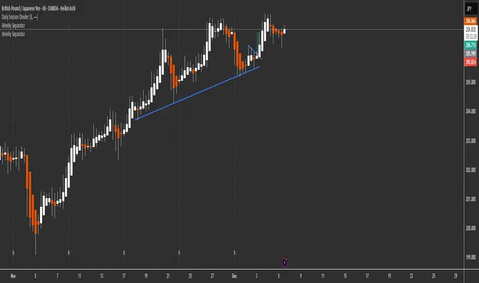
Weekly Separator - JammalWeekly Separator - Jammal
This script draws a clean and minimal weekly separator for better chart structure and visual clarity.
Every time a new trading week begins, the script automatically places a vertical dotted gray line extending across the entire chart.
Features:
Automatic weekly detection
Clean dotted vertical line
Light gray color to avoid clutter
Works on all timeframes
Helps identify weekly structure & price flow
Designed for traders who want a simple, non-intrusive weekly separator.
Enjoy and happy trading!
BTC STH Proxy vs Realized Price (RP) Ratio | STH : LTH📊 REALIZED PRICE MARKET SIGNAL
Indicator that builds a Short-Term Holder (STH) price proxy using a configurable moving average of Bitcoin’s market price and compares it to Bitcoin’s Realized Price (RP) derived from on-chain data.
Realized Price (RP) is calculated from CoinMetrics Realized Market Cap divided by Glassnode circulating supply.
STH Proxy is a user-defined moving average (EMA/SMA/WMA) of BTC price, designed to mimic the behavior of the true STH Realized Price.
Users can adjust the MA type, length, and RP smoothing to closely replicate the STH curve seen on Glassnode, Bitbo, and Bitcoin Magazine Pro.
Optionally, the indicator can display the STH/RP ratio, which highlights transitions between market phases.
This tool provides a simple but effective way to visualize short-term vs long-term holder cost-basis dynamics using only publicly accessible on-chain aggregates and price data.
----------
💡TLDR: An alt take on the Short-Term Holder Realized Price / Long-Term Holder Realized Price cross model | (STH/LTH cross)
- A mix of MAs are used to mimic STH.
- RP here used as a proxy for the long-term holder (LTH) cost basis.
- Bull/Bear signals are generated when the STH proxy crosses above or below RP.
⭐ Free to use • Leave feedback • Happy trading!

TMT Sessions - Hitesh NimjeTMT Sessions - Hitesh Nimje Indicator
Overview
The TMT Sessions indicator is a comprehensive trading tool designed to visualize and analyze the four major global trading sessions. It provides session-based technical analysis including ranges, trends, averages, and statistical metrics for each trading session.
Key Features
Four Global Trading Sessions
1. Session A - New York (13:00-22:00 UTC)
Color: Blue (#0000FF)
Default timeframe: US/Eastern market hours
2. Session B - London (07:00-16:00 UTC)
Color: Black (#000000)
Default timeframe: European market hours
3. Session C - Tokyo (00:00-09:00 UTC)
Color: Red (#FF0000)
Default timeframe: Asian market hours
4. Session D - Sydney (21:00-06:00 UTC)
Color: Orange (#FFA500)
Default timeframe: Australian market hours
Technical Analysis Tools
Range Analysis:
* Visual range boxes showing session high/low boundaries
* Transparent background areas with configurable transparency
* Range outline borders
* Session labels with customizable text display
Trend Analysis:
* Linear regression trendlines for each session
* Statistical metrics including:
R-squared values for trend strength
Standard deviation calculations
Correlation measurements
Statistical Indicators:
* Session Averages: Simple Moving Averages (SMA) calculated within each session
* VWAP: Volume Weighted Average Price for session-based intraday analysis
* Max/Min Lines: Highest and lowest prices recorded during each session
Visual Elements
Session Dividers:
* Visual markers showing session start/end points
* Session identification symbols (NYE, LDN, TYO, SYD)
* Configurable divider display options
Dashboard Features:
* Basic Dashboard: Session status (Active/Inactive) with color-coded indicators
* Advanced Dashboard: Additional metrics including:
Session trend strength (R-squared values)
Volume data
Standard deviation statistics
* Multiple dashboard positions (Top Right, Bottom Right, Bottom Left)
* Configurable text sizes (Tiny, Small, Normal)
Customization Options
Timezone Management:
* UTC offset adjustment (+/- hours)
* Exchange timezone option for automatic adjustment
* Session time customization
Display Settings:
* Individual session enable/disable
* Color customization for each session
* Range area transparency control
* Line description display toggle
* Session text label configuration
Use Cases
1. Session-Based Trading: Identify optimal trading times for each global session
2. Range Trading: Use session ranges as support/resistance levels
3. Trend Analysis: Track session-specific trends and momentum
4. Statistical Analysis: Monitor session volatility and trend strength
5. Market Structure: Understand how price moves across different trading sessions
Technical Specifications
* Pine Script Version: 6
* Overlays: True (displays on price chart)
* Performance: Optimized for up to 500 bars back
* Multi-element Support: Handles up to 500 lines, boxes, and labels
* Data Source: Compatible with all trading instruments and timeframes
Benefits for Traders
1. Global Market Awareness: Visual representation of all major trading sessions
2. Session Analysis: Automated calculation of key session statistics
3. Trading Strategy Development: Session-based entry and exit signals
4. Risk Management: Session ranges for stop-loss and take-profit levels
5. Market Timing: Optimal trading session identification
This indicator is particularly valuable for forex traders, day traders, and anyone who needs to understand price behavior across different global market sessions. It combines multiple technical analysis concepts into a unified, session-focused trading tool.
TRADING DISCLAIMER
RISK WARNING
Trading involves substantial risk of loss and is not suitable for all investors. Past performance is not indicative of future results. You should carefully consider whether trading is suitable for you in light of your circumstances, knowledge, and financial resources.
NO FINANCIAL ADVICE
This indicator is provided for educational and informational purposes only. It does not constitute:
* Financial advice or investment recommendations
* Buy/sell signals or trading signals
* Professional investment advice
* Legal, tax, or accounting guidance
LIMITATIONS AND DISCLAIMERS
Technical Analysis Limitations
* Pivot points are mathematical calculations based on historical price data
* No guarantee of accuracy of price levels or calculations
* Markets can and do behave irrationally for extended periods
* Past performance does not guarantee future results
* Technical analysis should be used in conjunction with fundamental analysis
Data and Calculation Disclaimers
* Calculations are based on available price data at the time of calculation
* Data quality and availability may affect accuracy
* Pivot levels may differ when calculated on different timeframes
* Gaps and irregular market conditions may cause level failures
* Extended hours trading may affect intraday pivot calculations
Market Risks
* Extreme market volatility can invalidate all technical levels
* News events, economic announcements, and market manipulation can cause gaps
* Liquidity issues may prevent execution at calculated levels
* Currency fluctuations, inflation, and interest rate changes affect all levels
* Black swan events and market crashes cannot be predicted by technical analysis
USER RESPONSIBILITIES
Due Diligence
* You are solely responsible for your trading decisions
* Conduct your own research before using this indicator
* Verify calculations with multiple sources before trading
* Consider multiple timeframes and confirm levels with other technical tools
* Never rely solely on one indicator for trading decisions
Risk Management
* Always use proper risk management and position sizing
* Set appropriate stop-losses for all positions
* Never risk more than you can afford to lose
* Consider the inherent risks of leverage and margin trading
* Diversify your portfolio and trading strategies
Professional Consultation
* Consult with qualified financial advisors before trading
* Consider your tax obligations and legal requirements
* Understand the regulations in your jurisdiction
* Seek professional advice for complex trading strategies
LIMITATION OF LIABILITY
Indemnification
The creator and distributor of this indicator shall not be liable for:
* Any trading losses, whether direct or indirect
* Inaccurate or delayed price data
* System failures or technical malfunctions
* Loss of data or profits
* Interruption of service or connectivity issues
No Warranty
This indicator is provided "as is" without warranties of any kind:
* No guarantee of accuracy or completeness
* No warranty of uninterrupted or error-free operation
* No warranty of merchantability or fitness for a particular purpose
* The software may contain bugs or errors
Maximum Liability
In no event shall the liability exceed the purchase price (if any) paid for this indicator. This limitation applies regardless of the theory of liability, whether contract, tort, negligence, or otherwise.
REGULATORY COMPLIANCE
Jurisdiction-Specific Risks
* Regulations vary by country and region
* Some jurisdictions prohibit or restrict certain trading strategies
* Tax implications differ based on your location and trading frequency
* Commodity futures and options trading may have additional requirements
* Currency trading may be regulated differently than stock trading
Professional Trading
* If you are a professional trader, ensure compliance with all applicable regulations
* Adhere to fiduciary duties and best execution requirements
* Maintain required records and reporting
* Follow market abuse regulations and insider trading laws
TECHNICAL SPECIFICATIONS
Data Sources
* Calculations based on TradingView data feeds
* Data accuracy depends on broker and exchange reporting
* Historical data may be subject to adjustments and corrections
* Real-time data may have delays depending on data providers
Software Limitations
* Internet connectivity required for proper operation
* Software updates may change calculations or functionality
* TradingView platform dependencies may affect performance
* Third-party integrations may introduce additional risks
MONEY MANAGEMENT RECOMMENDATIONS
Conservative Approach
* Risk only 1-2% of capital per trade
* Use position sizing based on volatility
* Maintain adequate cash reserves
* Avoid over-leveraging accounts
Portfolio Management
* Diversify across multiple strategies
* Don't put all capital into one approach
* Regularly review and adjust trading strategies
* Maintain detailed trading records
FINAL LEGAL NOTICES
Acceptance of Terms
* By using this indicator, you acknowledge that you have read and understood this disclaimer
* You agree to assume all risks associated with trading
* You confirm that you are legally permitted to trade in your jurisdiction
Updates and Changes
* This disclaimer may be updated without notice
* Continued use constitutes acceptance of any changes
* It is your responsibility to stay informed of updates
Governing Law
* This disclaimer shall be governed by the laws of the jurisdiction where the indicator was created
* Any disputes shall be resolved in the appropriate courts
* Severability clause: If any part of this disclaimer is invalid, the remainder remains enforceable
REMEMBER: THERE ARE NO GUARANTEES IN TRADING. THE MAJORITY OF RETAIL TRADERS LOSE MONEY. TRADE AT YOUR OWN RISK.
Contact Information:
* Creator: Hitesh_Nimje
* Phone: Contact@8087192915
* Source: Thought Magic Trading
© HiteshNimje - All Rights Reserved
This disclaimer should be prominently displayed whenever the indicator is shared, sold, or distributed to ensure users are fully aware of the risks and limitations involved in trading.

10% and 23.6% support bandsWhen a share is in momentum and showing lot of strength that relative strength it takes breather at 10% band from new 52 week high and and tends to consolidate at 23.6% from new 52 week high. This forms a higher low and gives opportunity to get in the rally. The volume bars should be taken into consideration as low volume and dry up at the bottom indicate reversal is coming. The stoploss for all entry is 1% below recent base low and entry pont is crossing of weekly high with greater than 20 days volume average.


The Floyd Sniper indicator1. tren; uses 200 EMA to decide bullish or bearish zone.
2. momentum; uses the 21EMA to confirm direction..
3. RSI filter; long only when oversold, Short only went overbought.
4. Signals; Prince long only when trend + momentum + RSI all Agree.
5. Background tent; green for long setups. red for short setups.

Altcoin Relative Macro StrengthAltcoin Relative Macro Strength
Overview
The Altcoin Relative Macro Strength indicator measures the altcoin market's price performance relative to global macroeconomic conditions. By comparing TOTAL3ES (total altcoin market capitalization excluding Bitcoin, Ethereum and stable coins) against a composite macro trend, the indicator identifies periods of relative overvaluation and undervaluation.
Methodology
Global Macro Trend Calculation:
The macro trend synthesizes three primary components:
- ISM PMI – A proxy for the business cycle phase
- Global Liquidity – An aggregate measure of major central bank balance sheets and broad money supply
- IWM (Russell 2000) – Small-cap equity exposure, reflecting risk-on/risk-off market sentiment
Global Liquidity is calculated as:
Fed Balance Sheet - Reverse Repo - Treasury General Account + U.S. M2 + China M2
The final Global Macro Trend is:
ISM PMI × Global Liquidity × IWM
Theoretical Framework:
The global macro trend integrates liquidity expansion/contraction with business cycle dynamics and small-cap equity performance. The inclusion of IWM reflects altcoins' tendency to behave as high-beta risk assets, exhibiting sensitivity similar to small-cap equities. This composite exhibits strong directional correlation with altcoin market movements, capturing the risk-on/risk-off dynamics that drive altcoin performance.
Interpretation
Primary Signal:
The histogram displays the rolling percentage change of TOTAL3ES relative to the global macro trend (default: 21-period average). Positive divergence indicates altcoins are outperforming macro conditions; negative divergence suggests underperformance relative to the underlying economic and risk environment.
Data Tables:
Alts/Macro Change – Percentage deviation of the altcoin market's average value from the Global Macro Trend's average over the specified period
Macro Trend – Directional assessment of the macro trend based on slope and trend agreement:
🔵 BULLISH ▲ – Positive slope with upward trend
⚪ NEUTRAL → – Slope and trend direction disagree
🟣 BEARISH ▼ – Negative slope with downward trend
Macro Slope – Percentage rate of change in the global macro trend
Altcoin Valuation – Relative valuation category based on TOTAL3/Macro deviation:
🟢 Extreme Discount / Deep Discount / Discount
🟡 Fair Value
🔴 Premium / Large Premium / Extreme Premium
TOTAL3ES Mcap – Current total altcoin market capitalization (in billions)
Visual Components:
📊 Histogram: Alts/Macro Change
🟢 Green = Positive deviation (altcoins outperforming)
🔴 Red = Negative deviation (altcoins underperforming)
📈 Macro Slope Line
Color-coded to match trend assessment
Scaled for visibility (adjustable in settings)
Application
This indicator is designed to identify mean reversion opportunities by highlighting periods when the altcoin market materially diverges from fundamental macro and risk conditions. Extreme positive values may indicate overvaluation; extreme negative values may signal undervaluation relative to the prevailing economic and risk appetite backdrop.
Strategy Considerations:
- Identify extremes: Look for periods when the histogram reaches elevated positive or negative levels
- Assess valuation: Use the Altcoin Valuation reading to gauge relative over/undervaluation
Confirm with risk sentiment: Check whether macro conditions and risk appetite support or contradict current price levels
- Mean reversion: Consider that significant deviations from trend historically tend to revert
Note: This indicator identifies relative valuation based on macro conditions and risk sentiment—it does not predict price direction or timing.
Settings
Lookback Period – 21 bars (default) – Number of bars for calculating rolling averages
Macro Slope Scale – 3.0 (default) – Multiplier for macro slope line visibility

Composite Market Momentum Indicator//@version=5
indicator("Composite Market Momentum Indicator", shorttitle="CMMI", overlay=false)
// Define Inputs
lenRSI = input.int(14, title="RSI Length")
lenMom = input.int(9, title="Momentum Length")
lenShortRSI = input.int(3, title="Short RSI Length")
lenShortRSISma = input.int(3, title="Short RSI SMA Length")
lenSMA1 = input.int(9, title="Composite SMA 1 Length")
lenSMA2 = input.int(34, title="Composite SMA 2 Length")
// Step 1: Create a 9-period momentum indicator of the 14-period RSI
rsiValue = ta.rsi(close, lenRSI)
momRSI = ta.mom(rsiValue, lenMom)
// Step 2: Create a 3-period RSI and a 3-period SMA of that RSI
shortRSI = ta.rsi(close, lenShortRSI)
shortRSISmoothed = ta.sma(shortRSI, lenShortRSISma)
// Step 3: Add Step 1 and Step 2 together to create the Composite Index
compositeIndex = momRSI + shortRSISmoothed
// Step 4: Create two simple moving averages of the Composite Index
sma1 = ta.sma(compositeIndex, lenSMA1)
sma2 = ta.sma(compositeIndex, lenSMA2)
// Step 5: Plot the composite index and its two simple moving averages
plot(compositeIndex, title="Composite Index", color=color.new(#f7cf05, 0), linewidth=2)
plot(sma1, title="SMA 13", color=color.new(#f32121, 0), linewidth=1, style=plot.style_line)
plot(sma2, title="SMA 33", color=color.new(#105eef, 0), linewidth=1, style=plot.style_line)
// Add horizontal lines for reference
hline(0, "Zero Line", color.new(color.gray, 50))

XAUUSD Liquidity Sweep + Engulfing (4H/2H/15m)Key Features in This Script:
4H Bias (Trend): We use RSI on 4H to determine if the market is in a bullish or bearish trend.
2H Setup: When price sweeps below previous lows or above previous highs (liquidity sweep), we confirm it with RSI and an engulfing candle.
15m Entry: After the liquidity sweep is confirmed on the 15m chart, we check for a bullish engulfing (for buys) or bearish engulfing (for sells) with RSI confirmation.
How to Use It:
Add the Script: Copy-paste the code above into TradingView’s Pine Editor.
Apply it to the 15-minute chart for XAUUSD (Gold).
Alerts: Set up alerts when a Buy or Sell signal appears based on the conditions.
Alerts Example:
When a liquidity sweep and RSI flip happens with an engulfing candle, TradingView will notify you, helping you enter at the right time.
🚀 Next Steps:
Try it out and let me know how the alerts and signals are working for you.
If you'd like to add custom stop-loss or take-profit calculations, or include Fibonacci levels, let me know!

Baba-pro EMA Break Sniper This indicator is designed to provide high-precision entries based on the interaction between EMAs, momentum, and clean price breaks.
Instead of relying on traditional EMA crossovers — which are often too slow — this tool focuses on direct EMA breakouts, allowing you to catch moves before most traders even react.

SPX Breadth – Stocks Above 200-day SMA//@version=6
indicator("SPX Breadth – Stocks Above 200-day SMA",
overlay = false,
max_lines_count = 500,
max_labels_count = 500)
//–––––––––––––––––––––––––––––––––––––––––––––––––––––––––––––––––––––––––––––
// Inputs
group_source = "Source"
breadthSymbol = input.symbol("SPXA200R", "Breadth symbol", group = group_source)
breadthTf = input.timeframe("", "Timeframe (blank = chart)", group = group_source)
group_params = "Parameters"
totalStocks = input.int(500, "Total stocks in index", minval = 1, group = group_params)
smoothingLen = input.int(10, "SMA length", minval = 1, group = group_params)
//–––––––––––––––––––––––––––––––––––––––––––––––––––––––––––––––––––––––––––––
// Breadth series (symbol assumed to be percent 0–100)
string tf = breadthTf == "" ? timeframe.period : breadthTf
float rawPct = request.security(breadthSymbol, tf, close) // 0–100 %
float breadthN = rawPct / 100.0 * totalStocks // convert to count
float breadthSma = ta.sma(breadthN, smoothingLen)
//–––––––––––––––––––––––––––––––––––––––––––––––––––––––––––––––––––––––––––––
// Regime levels (0–20 %, 20–40 %, 40–60 %, 60–80 %, 80–100 %)
float lvl0 = 0.0
float lvl20 = totalStocks * 0.20
float lvl40 = totalStocks * 0.40
float lvl60 = totalStocks * 0.60
float lvl80 = totalStocks * 0.80
float lvl100 = totalStocks * 1.0
p0 = plot(lvl0, "0%", color = color.new(color.black, 100))
p20 = plot(lvl20, "20%", color = color.new(color.red, 0))
p40 = plot(lvl40, "40%", color = color.new(color.orange, 0))
p60 = plot(lvl60, "60%", color = color.new(color.yellow, 0))
p80 = plot(lvl80, "80%", color = color.new(color.green, 0))
p100 = plot(lvl100, "100%", color = color.new(color.green, 100))
// Colored zones
fill(p0, p20, color = color.new(color.maroon, 80)) // very oversold
fill(p20, p40, color = color.new(color.red, 80)) // oversold
fill(p40, p60, color = color.new(color.gold, 80)) // neutral
fill(p60, p80, color = color.new(color.green, 80)) // bullish
fill(p80, p100, color = color.new(color.teal, 80)) // very strong
//–––––––––––––––––––––––––––––––––––––––––––––––––––––––––––––––––––––––––––––
// Plots
plot(breadthN, "Stocks above 200-day", color = color.orange, linewidth = 2)
plot(breadthSma, "Breadth SMA", color = color.white, linewidth = 2)
// Optional label showing live value
var label infoLabel = na
if barstate.islast
label.delete(infoLabel)
string txt = "Breadth: " +
str.tostring(breadthN, format.mintick) + " / " +
str.tostring(totalStocks) + " (" +
str.tostring(rawPct, format.mintick) + "%)"
infoLabel := label.new(bar_index, breadthN, txt,
style = label.style_label_left,
color = color.new(color.white, 20),
textcolor = color.black)

Z-score RegimeThis indicator compares equity behaviour and credit behaviour by converting both into z-scores. It calculates the z-score of SPX and the z-score of a credit proxy based on the HYG divided by LQD ratio.
SPX z-score shows how far the S&P 500 is from its rolling average.
Credit z-score shows how risk-seeking or risk-averse credit markets are by comparing high-yield bonds to investment-grade bonds.
When both z-scores move together, the market is aligned in either risk-on or risk-off conditions.
When SPX z-score is strong but credit z-score is weak, this may signal equity strength that is not supported by credit markets.
When credit z-score is stronger than SPX z-score, credit markets may be leading risk appetite.
The indicator plots the two z-scores as simple lines for clear regime comparison.

CCI TIME COUNT//@version=6
indicator("CCI Multi‑TF", overlay=true)
// === Inputs ===
// CCI Inputs
cciLength = input.int(20, "CCI Length", minval=1)
src = input.source(hlc3, "Source")
// Timeframes
timeframes = array.from("1", "3", "5", "10", "15", "30", "60", "1D", "1W")
labels = array.from("1m", "3m", "5m", "10m", "15m", "30m", "60m", "Daily", "Weekly")
// === Table Settings ===
tblPos = input.string('Top Right', 'Table Position', options = , group = 'Table Settings')
i_textSize = input.string('Small', 'Text Size', options = , group = 'Table Settings')
textSize = i_textSize == 'Small' ? size.small : i_textSize == 'Normal' ? size.normal : i_textSize == 'Large' ? size.large : size.tiny
textColor = color.white
// Resolve table position
var pos = switch tblPos
'Top Left' => position.top_left
'Top Right' => position.top_right
'Bottom Left' => position.bottom_left
'Bottom Right' => position.bottom_right
'Middle Left' => position.middle_left
'Middle Right' => position.middle_right
=> position.top_right
// === Custom CCI Function ===
customCCI(source, length) =>
sma = ta.sma(source, length)
dev = ta.dev(source, length)
(source - sma) / (0.015 * dev)
// === CCI Values for All Timeframes ===
var float cciVals = array.new_float(array.size(timeframes))
for i = 0 to array.size(timeframes) - 1
tf = array.get(timeframes, i)
cciVal = request.security(syminfo.tickerid, tf, customCCI(src, cciLength))
array.set(cciVals, i, cciVal)
// === Countdown Timers ===
var string countdowns = array.new_string(array.size(timeframes))
for i = 0 to array.size(timeframes) - 1
tf = array.get(timeframes, i)
closeTime = request.security(syminfo.tickerid, tf, time_close)
sec_left = barstate.isrealtime and not na(closeTime) ? math.max(0, (closeTime - timenow) / 1000) : na
min_left = sec_left >= 0 ? math.floor(sec_left / 60) : na
sec_mod = sec_left >= 0 ? math.floor(sec_left % 60) : na
timer_text = barstate.isrealtime and not na(sec_left) ? str.format("{0,number,00}:{1,number,00}", min_left, sec_mod) : "–"
array.set(countdowns, i, timer_text)
// === Build Table ===
if barstate.islast
rows = array.size(timeframes) + 1
var table t = table.new(pos, 3, rows, frame_color=color.rgb(252, 250, 250), border_color=color.rgb(243, 243, 243))
// Headers
table.cell(t, 0, 0, "Timeframe", text_color=textColor, bgcolor=color.rgb(238, 240, 242), text_size=textSize)
table.cell(t, 1, 0, "CCI (" + str.tostring(cciLength) + ")", text_color=textColor, bgcolor=color.rgb(239, 243, 246), text_size=textSize)
table.cell(t, 2, 0, "Time to Close", text_color=textColor, bgcolor=color.rgb(239, 244, 248), text_size=textSize)
// Data Rows
for i = 0 to array.size(timeframes) - 1
row = i + 1
label = array.get(labels, i)
cciVal = array.get(cciVals, i)
countdown = array.get(countdowns, i)
// Color CCI: Green if < -100, Red if > 100
cciColor = cciVal < -100 ? color.green : cciVal > 100 ? color.red : color.rgb(236, 237, 240)
// Background warning if <60 seconds to close
tf = array.get(timeframes, i)
closeTime = request.security(syminfo.tickerid, tf, time_close)
sec_left = barstate.isrealtime and not na(closeTime) ? math.max(0, (closeTime - timenow) / 1000) : na
countdownBg = sec_left < 60 ? color.rgb(255, 220, 220, 90) : na
// Table cells
table.cell(t, 0, row, label, text_color=color.rgb(239, 240, 244), text_size=textSize)
table.cell(t, 1, row, str.tostring(cciVal, "#.##"), text_color=cciColor, text_size=textSize)
table.cell(t, 2, row, countdown, text_color=color.rgb(232, 235, 243), bgcolor=countdownBg, text_size=textSize)

Jon Secret SauceJon Secret Sauce — Advanced Trend + Momentum Entry Signals
A premium trade-timing engine that combines MA trend confirmation, volatility filters, RSI momentum, and smart volume validation to identify high-probability long & short entries on your preferred timeframe.
Includes auto-managed exits (TP / SL / technical breakdown), professional visuals, and alert notifications so you catch the move and protect profits — without overcrowding your chart.

Momentum Structural AnalysisMomentum Structural Analysis (MSA‑style Oscillator)
This indicator implements a simple, MSA‑style momentum oscillator that measures how far price has moved above or below its own long‑term trend on the active timeframe, expressed in percentage terms. Instead of looking at raw price, it "oscillates" price around a timeframe‑appropriate simple moving average (SMA) and plots the percentage distance from that SMA as an orange line around a zero baseline. Zero means price is exactly at its structural trend; positive values mean price is extended above trend; negative values mean it is trading below trend.
The script automatically selects the SMA length based on the chart timeframe:
On daily charts it uses the configurable Daily SMA Length (default 252 trading days, roughly 1 year).
On weekly charts it uses Weekly SMA Length (default 208 weeks).
On monthly charts it uses Monthly SMA Length (default 120 months).
This approach is inspired by the ideas behind Momentum Structural Analysis (MSA), which studies where a market trades relative to long‑term moving averages and then treats the momentum line (the oscillator) as the primary object of analysis. The goal is to highlight structural overbought/oversold conditions and regime changes that are often clearer on momentum than on the raw price chart.
--------------------------------------------------
What the script computes and how it works
For each bar, the indicator:
Chooses an SMA length based on the current timeframe (daily/weekly/monthly).
Calculates the SMA of the close.
Computes the percentage distance:
\text{Diff %} = \frac{\text{Close} - \text{SMA}}{\text{SMA}} \times 100
Plots this Diff % as an orange line, with a dashed horizontal zero line as the base.
This produces a momentum oscillator that oscillates around zero and reflects the "structural" position of price versus its own long‑term mean.
--------------------------------------------------
How to use it on index charts (e.g., NIFTY50)
On indices like NIFTY50, use the indicator to see how stretched the index is versus its structural trend.
Typical uses:
Identify extremes: a). Historically high positive readings can signal euphoric, late‑stage conditions where risk is elevated. b). Deep negative readings can highlight panic/capitulation zones where downside may be exhausted.
Draw structural levels: a). Mark horizontal bands on the oscillator where past turns have occurred (e.g., +15%, −10%, etc. specific to NIFTY50). b). Watch how price behaves when the oscillator revisits these zones: repeated rejections can validate them as structural bounds; clean breaks can indicate a change of regime.
This is not a buy/sell signal generator by itself; it is a framework to understand where the index sits within its long‑term momentum structure and to support risk‑management decisions.
--------------------------------------------------
How to use it on ratio charts
Apply the same indicator to ratio symbols such as NIFTY50/GOLD, BANKNIFTY/NIFTY50, sector vs index, or any spread you plot as a ratio.
On a ratio chart:
The oscillator now measures relative momentum: how far that ratio is above or below its own long‑term mean.
High positive readings = strong outperformance of the numerator vs the denominator (e.g., equities strongly outperforming gold).
Deep negative readings = strong underperformance (e.g., equities structurally lagging gold).
This is very much in the spirit of MSA’s work on spreads between asset classes: it helps visualize major rotations (equities → gold, financials → commodities, etc.) and whether a relative‑performance trend is stretched, reverting, or breaking into a new phase.
--------------------------------------------------
Using multiple timeframes for better decisions
You can stack information across timeframes to get a more robust view:
Monthly : a). Use monthly charts to see secular/structural phases. b). Long multi‑year stretches above or below zero, and large bases or trendline breaks on the monthly oscillator, can mark major bull or bear cycles and big rotations between asset classes.
Weekly : a). Use weekly charts for the primary trend. b). Weekly structures (multi‑month highs/lows, channels, or trendlines on the oscillator) are useful for medium‑term positioning and for confirming or rejecting signals seen on the monthly view.
Daily : a). Use daily charts mainly for timing entries/exits once the higher‑timeframe direction is clear. b). Short‑term extremes on the daily oscillator that align with the larger weekly/monthly structure can offer better‑timed opportunities, while signals that contradict higher‑timeframe momentum are more likely to be noise.
--------------------------------------------------

Advanced ICC Multi-Timeframe 1.0Advanced ICC Multi-Timeframe Trading System
A comprehensive implementation and interpretation of the Indication, Correction, Continuation (ICC) trading methodology made popular by Trades by Sci, enhanced with advanced multi-timeframe analysis and automation features.
⚠️ CRITICAL TRADING WARNINGS:
DO NOT blindly follow BUY/SELL signals from this indicator
This indicator shows potential entry points but YOU must validate each trade
PAPER TRADE EXTENSIVELY before risking real capital
BACKTEST THOROUGHLY on your chosen instruments and timeframes
The ICC methodology requires understanding and discretion - automated signals are guidance only
This tool aids analysis but does not replace proper trade planning, risk management, or trader judgment
⚠️ Important Disclaimers:
This indicator is not endorsed by or affiliated with Trades by Sci
This is an early implementation and interpretation of the ICC methodology
May not work exactly as Trades by Sci executes his trades and entries
Requires further debugging, backtesting, and real-world validation
Completely free to use - no purchase required
I'm just one person obsessed with this method and wanted some better visualization of the chart/entries
About ICC:
The ICC method identifies complete market cycles through three phases: Indication (breakout), Correction (pullback), and Continuation (entry). This indicator automates the identification of these phases and adds powerful features for modern traders.
Key Features:
Multi-Timeframe Capabilities:
Automatic timeframe detection with optimized settings for 5m, 15m, 30m, 1H, 4H, and Daily charts
Higher timeframe overlay to view HTF ICC levels on lower timeframe charts for precise entry timing
Smart defaults that adjust swing length and consolidation detection based on your timeframe
Advanced Phase Tracking:
Complete ICC cycle tracking: Indication, Correction, Consolidation, Continuation, and No Setup phases
Live structure detection shows potential peaks/troughs before full confirmation
Intelligent invalidation logic detects failed setups when market structure reverses
Dynamic phase backgrounds for instant visual confirmation
Three Types of Entry Signals:
Traditional Entries - Price crosses back through the original indication level (strongest signals)
"BUY" (green) / "SELL" (red)
Breakout Entries - Price breaks out of consolidation range in the same direction
"BUY" (green) / "SELL" (red)
Reversal Entries (Optional, can be toggled off) - Price breaks consolidation in opposite direction, indicating failed setup
"⚠ BUY" (yellow) / "⚠ SELL" (orange)
More aggressive, counter-trend signals
Can be disabled for more conservative trading
Professional Features:
Volatility-based support/resistance zones (ATR-adjusted) that adapt to market conditions
Historical zone tracking (0-3 configurable) with visual hierarchy
Comprehensive real-time info table displaying all key metrics
Full alert system for entries, indications, and consolidation detection
Visual distinction between high-confidence trend entries and cautionary reversal entries
📖 USAGE GUIDE
Entry Signal Types:
The indicator provides three types of entry signals with visual distinction:
Strong Entries (High Confidence):
"BUY" (bright green) / "SELL" (bright red)
Includes traditional entries (crossing back through indication level) and breakout entries (breaking consolidation in trend direction)
These are trend continuation or breakout signals with higher probability
Recommended for all traders
Reversal Entries (Caution - Counter-Trend):
"⚠ BUY" (yellow) / "⚠ SELL" (orange)
Triggered when price breaks out of correction/consolidation in the OPPOSITE direction
Indicates a failed setup and potential trend reversal
More aggressive, counter-trend plays
Can be toggled off in settings for more conservative trading
Recommended only for experienced traders or after thorough backtesting
Swing Length Settings:
The swing length determines how many bars on each side are needed to confirm a swing high/low. This is the most important setting for tuning the indicator to your style.
Auto Mode (Recommended for beginners): Toggle "Use Auto Timeframe Settings" ON
5-minute: 30 bars
15-minute: 20 bars
30-minute: 12 bars
1-hour: 7 bars
4-hour: 5 bars
Daily: 3 bars
Manual Mode: Toggle "Use Auto Timeframe Settings" OFF
Lower values (3-7): More aggressive, detects smaller swings
Pros: More signals, faster entries, catches smaller moves
Cons: More noise, more false signals, requires tighter stops
Best for: Scalping, active day trading, volatile markets
Higher values (12-20): More conservative, only major swings
Pros: More reliable signals, fewer false breakouts, clearer structure
Cons: Fewer signals, delayed entries, might miss smaller opportunities
Best for: Swing trading, position trading, trending markets
Default Manual Setting: 7 bars (balanced for 1H charts)
Minimum: 3 bars
Consolidation Bars Setting:
Determines how many bars without new structure are needed before flagging consolidation.
Lower values (3-10): Faster detection, catches brief pauses, more sensitive
Best for: Lower timeframes, volatile markets, avoiding any chop
Higher values (20-40): More reliable, only flags true extended consolidation
Best for: Higher timeframes, trending markets, patient traders
Current defaults scale with timeframe (more bars needed on shorter timeframes)
Historical S/R Zones:
Shows previous support and resistance levels to provide context.
Default: 2 historical zones (shows current + 2 previous)
Range: 0-3 zones
Visual Hierarchy: Older zones are more transparent with dashed borders
Usage: Higher numbers (2-3) show more historical context but can clutter the chart. Start with 2 and adjust based on your preference.
Live Structure Feature (Yellow Warning ⚠):
Provides early warning of potential structure changes before full confirmation.
What it does: Detects potential swing highs/lows after just 2 bars instead of waiting for full swing_length confirmation
Live Peak: Shows when a high is followed by 2 lower closes (potential top forming)
Live Trough: Shows when a low is followed by 2 higher closes (potential bottom forming)
Important: These are UNCONFIRMED - they may be invalidated if price reverses
Use case: Get early awareness of potential reversals while waiting for confirmation
Displayed in: Info table only (no visual markers on chart to reduce clutter)
Only shows: Peaks higher than last swing high, or troughs lower than last swing low (filters out noise)
Higher Timeframe (HTF) Analysis:
View higher timeframe ICC structure while trading on lower timeframes.
How to enable: Toggle "Show Higher Timeframe ICC" ON
Setup: Set "Higher Timeframe" to your reference timeframe
Example: Trading on 15-minute? Set HTF to 240 (4-hour) or 60 (1-hour)
Example: Trading on 5-minute? Set HTF to 60 (1-hour) or 15 (15-minute)
What it shows:
HTF indication levels displayed as dashed lines
Blue = HTF Bullish Indication
Purple = HTF Bearish Indication
HTF phase and levels shown in info table
Trading workflow:
Check HTF phase for overall market direction
Wait for HTF correction phase
Drop to lower timeframe to find precise entries
Enter when lower TF shows continuation in alignment with HTF
Best practice: HTF should be 3-4x your trading timeframe for best results
Reversal Entries Toggle:
Default: ON (shows all signal types)
Toggle OFF for more conservative trading (only trend continuation signals)
Recommended: Backtest with both settings to see which works better for your style
New traders should consider disabling reversal entries initially
Volatility-Based Zones:
When enabled, support/resistance zones automatically adjust their height based on ATR (Average True Range).
More volatile = wider zones
Less volatile = tighter zones
Toggle OFF for fixed-width zones
Community Feedback Welcome:
This is an evolving project and your input is valuable! Please share:
Bug reports and issues you encounter
Feature requests and suggestions for improvement
Results from your backtesting and live trading experience
Feedback on the reversal entry feature (too aggressive? working well?)
Ideas for better aligning with the ICC methodology
Perfect for traders learning or implementing the ICC methodology with the benefit of modern automation, multi-timeframe analysis, and flexible entry signal options.

BTC – LEVR: Leverage Efficiency & Volume RatioLEVR: Leverage Efficiency & Volume Ratio
Observation-only. Data: IntoTheBlock.
Overview
The Leverage Efficiency & Volume Ratio (LEVR) is a market structure oscillator designed to detect "Paper Bubbles" and "Organic Bottoms" by separating speculative greed from network utility. While most indicators analyze price action, LEVR analyzes market fragility. It operates on the thesis that Sustainable Rallies are driven by Spot/Network Activity, while Fragile Rallies are driven by Derivatives Leverage.
Synergy
How it works with VERI
LEVR is designed to be the tactical counterpart to the fundamental VERI Indicator (Valuation & Entity Ratio Index).
Use VERI for Strategy: To identify Value. (Is Bitcoin cheap? Are Whales buying?)
Use LEVR for Risk: To identify Structure. (Is the current price move real, or is it a leverage bubble about to pop?)
The "Perfect Setup"
The strongest buy signals occur when VERI is in the Accumulation Zone (Whales buying) AND LEVR is in the Organic Zone (Leverage is flushed out) (as it was the case in the Dec 2022 Bear Market Bottom).
Why LEVR is Unique
Standard indicators often fail to contextualize Open Interest:
vs. Raw Open Interest: Raw OI always trends up over time as the market grows. LEVR solves this by normalizing OI against Active Addresses. This reveals when leverage is outpacing actual adoption.
vs. ELR (Estimated Leverage Ratio): Classic ELR divides Open Interest by Exchange Reserves. However, Exchange Reserves are notoriously difficult to track accurately. LEVR uses Active Addresses (Network Utility) as a cleaner, more reliable denominator for network health.
Methodology
The Mathematics: The indicator calculates a normalized Z-Score ratio between two IntoTheBlock datasets:
The Numerator (Greed): Perpetual Open Interest. The total dollar value of all open futures contracts. This represents the "Gambling" capital.
The Denominator (Utility): Active Addresses. The number of unique addresses transacting on-chain. This represents the "Real" user base.
The Formula : LEVR = Z-Score ( Perpetual Open Interest / Active Addresses )
How to Interpret the Visuals
The line color changes dynamically to reflect the current risk regime:
🟥 Speculative Premium (Red Line > 2.0) :
Signal: "Leverage Bubble."
Context: Open Interest is rising significantly faster than User Growth. The rally is fueled by debt.
Risk: High probability of a "Long Squeeze" or liquidation cascade.
🟦 Organic Base (Blue Line < -1.5) :
Signal: "Spot Driven Market."
Context: Speculators have been flushed out, but active network usage remains high. The line turns Blue to signal a healthy opportunity zone.
Risk: Low. Historically marks robust bottoms where hands are strong.
🟧 Neutral (Orange Line) :
The market is in a transition phase between organic growth and speculation.
Settings & Inputs
Users can customize the sensitivity of the Z-Score to fit their trading style (in brackets their current standard value):
Lookback Period (365) : The rolling window used to establish the "Baseline." A 365-day window captures the yearly trend.
Signal Smoothing (7) : A short moving average to reduce daily data noise.
Bubble Zone Top/Bottom (3.0 / 2.0) : The thresholds for the Red Zone. Raising the "Top" value will only show the most extreme, generational leverage bubbles.
Organic Zone Top/Bottom (-1.5 / -2.5) : The thresholds for the Green Zone. Lowering these values requires a deeper "flush" to trigger a signal.
Optimization
This indicator is mathematically optimized for the Daily (1D) timeframe. Using it on lower timeframes may result in noise due to the daily resolution of on-chain data.
Important Note on Historical Data
Please be aware that aggregated global Perpetual Open Interest data only becomes reliable and widely available starting around 2020-2021.
Pre-2021: The indicator will show a flat line or empty values. This is not a bug; it reflects the lack of historical derivatives market data for that period.
2021-Present: The indicator functions fully as intended.
Credits
Concept inspired by the "Estimated Leverage Ratio" (ELR) popularised by CryptoQuant and analysts like Willy Woo. LEVR adapts this concept for TradingView by substituting Exchange Reserves with Network Activity for better reliability.
Disclaimer
This tool is for research purposes only. It visualizes market structure data and does not constitute financial advice.
Tags
bitcoin, btc, open interest, leverage, on-chain, intotheblock, risk, derivatives, levr, veri

One for AllOne for All (OFA) - Complete ICT Analysis Suite
Version 3.3.0 by theCodeman
📊 Overview
One for All (OFA) is a comprehensive TradingView indicator designed for traders who follow Inner Circle Trader (ICT) concepts. This all-in-one tool combines essential ICT analysis features—sessions, kill zones, previous period levels, and higher timeframe candles with Fair Value Gaps (FVGs) and Volume Imbalances (VIs)—into a single, highly customizable indicator. Whether you're a beginner learning ICT concepts or an experienced trader refining your edge, OFA provides the visual structure needed for precise market analysis and execution.
✨ Key Features
- 🏷️ Customizable Watermark**: Display your trading identity with customizable titles, subtitles, symbol info, and full style control
- 🌍 Trading Sessions**: Visualize Asian, London, and New York sessions with high/low lines, range boxes, and open/close markers
- 🎯 Kill Zones**: Highlight 5 critical ICT kill zones with precise timing and visual boxes
- 📈 Previous Period H/L**: Track Daily, Weekly, and Monthly highs/lows with customizable styles and lookback periods
- 🕐 Higher Timeframe Candles**: Display up to 5 HTF timeframes with OHLC trace lines, timers, and interval labels
- 🔍 FVG & VI Detection**: Automatically detect and visualize Fair Value Gaps and Volume Imbalances on HTF candles
- ⚙️ Universal Timezone Support**: Works globally with GMT-12 to GMT+14 timezone selection
- 🎨 Full Customization**: Control colors, styles, visibility, and layout for every feature
🚀 How to Use
Watermark Setup
The watermark overlay helps you identify your charts and maintain focus on your trading principles:
1. Enable/disable watermark via "Show Watermark" toggle
2. Customize the title (default: "Name") to display your trading name or account identifier
3. Set up to 3 subtitles (default: "Patience", "Confidence", "Execution") as trading reminders
4. Choose position (9 locations available), size, color, and transparency
5. Toggle symbol and timeframe display as needed
Use Case: Display your trading principles or account name for multi-monitor setups or content creation.
Trading Sessions Analysis
Sessions define market character and liquidity availability:
1. Enable "Show All Sessions" to visualize all three sessions
2. Adjust timezone to match your local market (default: UTC-5 for EST)
3. Customize session times if needed (defaults cover standard hours)
4. Enable session range boxes to see consolidation zones
5. Use session high/low lines to identify key levels for the current session
6. Enable open/close markers to track session transitions
Use Case: Identify which session you're trading in, track session highs/lows for liquidity, and anticipate session transition volatility.
Kill Zones Trading
Kill zones are ICT's high-probability trading windows:
1. Enable individual kill zones or use "Show All Kill Zones"
2. **Asian Kill Zone** (2000-0000 GMT): Early positioning and smart money accumulation
3. **London Kill Zone** (0300-0500 GMT): European market opening volatility
4. **NY AM Kill Zone** (0930-1100 EST): Post-NYSE open expansion
5. **NY Lunch Kill Zone** (1200-1300 EST): Midday consolidation or manipulation
6. **NY PM Kill Zone** (1330-1600 EST): Afternoon positioning and closes
7. Customize colors and times to match your trading style
8. Set max days display to control historical visibility (default: 30 days)
Use Case: Focus entries during high-probability windows. Watch for liquidity sweeps at kill zone openings and institutional positioning.
Previous Period High/Low Levels
Previous period levels act as magnetic price targets and support/resistance:
1. Enable Daily (PDH/PDL), Weekly (PWH/PWL), or Monthly (PMH/PML) levels individually
2. Set lookback period (how many previous periods to display)
3. Choose line style: Solid (current emphasis), Dashed (standard), or Dotted (subtle)
4. Customize colors per timeframe for visual hierarchy
5. Adjust line width (1-5) for visibility preference
6. Enable gradient effect to fade older periods
7. Position labels left or right based on chart layout
8. Customize label text for your preferred notation
Use Case: Identify key levels where price is likely to react. Daily levels work on intraday timeframes, Weekly on daily charts, Monthly for swing trading.
Higher Timeframe (HTF) Candles
HTF candles reveal the larger market context while trading lower timeframes:
1. Enable up to 5 HTF slots simultaneously (default: 5m, 15m, 1H, 4H, Daily)
2. Choose display mode: "Below Chart" (stacked rows) or "Right Side" (compact column)
3. Customize timeframe, colors (bull/bear), and titles for each slot
4. **OHLC Trace Lines**: Visual lines connecting HTF candle levels to chart bars
5. **HTF Timer**: Countdown showing time remaining until HTF candle close
6. **Interval Labels**: Display day of week (Daily+) or time (intraday) on each candle
7. For Daily candles: Choose open time (Midnight, 8:30, 9:30) to match your market structure preference
Use Case: Trade lower timeframes while respecting higher timeframe structure. Watch for HTF candle closes to confirm directional bias.
FVG & VI Detection
Fair Value Gaps and Volume Imbalances highlight inefficiencies that price often revisits:
1. **Fair Value Gaps (FVGs)**: Detected when HTF candle wicks don't overlap between 3 consecutive candles
- Bullish FVG: Gap between candle 1 high and candle 3 low (green box by default)
- Bearish FVG: Gap between candle 1 low and candle 3 high (red box by default)
2. **Volume Imbalances (VIs)**: Similar detection but focuses on body gaps
- Bullish VI: Gap between candle 1 close and candle 3 open
- Bearish VI: Gap between candle 1 open and candle 3 close
3. Enable FVG/VI detection per HTF slot individually
4. Customize colors and transparency for each imbalance type
5. Boxes appear on chart at formation and remain visible as retracement targets
**Use Case**: Identify high-probability retracement zones. Price often returns to fill FVGs and VIs before continuing the trend. Use as entry zones or profit targets.
🎨 Customization
OFA is built for flexibility. Every feature includes extensive customization options:
Visual Customization
- **Colors**: Independent color control for every element (sessions, kill zones, lines, labels, FVGs, VIs)
- **Transparency**: Adjust box and label transparency (0-100%) for clean charts
- **Line Styles**: Choose Solid, Dashed, or Dotted for previous period lines
- **Sizes**: Control text size, line width, and box borders
- **Positions**: Place watermark in 9 positions, labels left/right
Layout Control
- **HTF Display Mode**: "Below Chart" for detailed analysis, "Right Side" for space efficiency
- **Drawing Limits**: Set max days for sessions/kill zones to manage chart clutter
- **Lookback Periods**: Control how many previous periods to display (1-10)
- **Gradient Effects**: Enable fading for older previous period lines
Timing Adjustments
- **Timezone**: Universal GMT offset selector (-12 to +14) for global markets
- **Session Times**: Customize each session's start/end times
- **Kill Zone Times**: Adjust kill zone windows to match your market's characteristics
- **Daily Open**: Choose Midnight, 8:30, or 9:30 for Daily HTF candle open time
💡 Best Practices
1. Start Simple: Enable one feature at a time to learn how each element affects your analysis
2. Match Your Timeframe: Use Daily levels on intraday charts, Weekly on daily charts, HTF candles one or two levels above your trading timeframe
3. Kill Zone Focus: Concentrate your trading activity during kill zones for higher probability setups
4. HTF Confirmation: Wait for HTF candle closes before committing to directional bias
5. FVG/VI Entries: Look for price to return to unfilled FVGs/VIs for entry opportunities with favorable risk/reward
6. Customize Colors: Use a consistent color scheme that matches your chart theme and reduces visual fatigue
7. Reduce Clutter: Disable features you're not actively using in your current trading plan
8. Session Context: Understand which session controls the market—trade with session direction or anticipate reversals at session transitions
⚙️ Settings Guide
OFA organizes settings into logical groups for easy navigation:
- **═══ WATERMARK ═══**: Title, subtitles, position, style, symbol/timeframe display
- **═══ SESSIONS ═══**: Enable/disable sessions, times, colors, high/low lines, boxes, markers
- **═══ KILL ZONES ═══**: Individual kill zone toggles, times, colors, max days display
- **═══ PREVIOUS H/L - DAILY ═══**: Daily high/low lines, style, color, lookback, labels
- **═══ PREVIOUS H/L - WEEKLY ═══**: Weekly high/low lines, style, color, lookback, labels
- **═══ PREVIOUS H/L - MONTHLY ═══**: Monthly high/low lines, style, color, lookback, labels
- **═══ HTF CANDLES ═══**: Global display mode, layout settings
- **═══ HTF SLOT 1-5 ═══**: Individual HTF configuration (timeframe, colors, title, FVG/VI detection, trace lines, timer, interval labels)
Each setting includes tooltips explaining its function. Hover over any input for detailed guidance.
📝 Final Notes
One for All (OFA) represents a complete ICT analysis toolkit in a single indicator. By combining watermark customization, session visualization, kill zone highlighting, previous period levels, and higher timeframe candles with FVG/VI detection, OFA eliminates the need for multiple indicators cluttering your chart.
**Version**: 3.3.0
**Author**: theCodeman
**Pine Script**: v6
**License**: Mozilla Public License 2.0
Start with default settings to learn the indicator's structure, then customize extensively to match your personal trading style. Remember: tools provide information, but your edge comes from disciplined execution of a proven strategy.
Happy Trading! 📈

BTC - VERI - Valuation & Entity Ratio IndexVERI: Valuation & Entity Ratio IndexObservation-only.
Data: IntoTheBlock.
Overview & Philosophy
The name VERI is derived from the Latin Veritas (Truth). In a crypto market often driven by deceptive speculative noise, this indicator seeks to establish the "On-Chain Truth" of a price trend.
It operates on the thesis that price action is only sustainable when verified by high-conviction capital flows.VERI is a fundamental composite oscillator that fuses Entity Behavior (Who is holding?) with Network Valuation (Is the price fair?) to identify Bitcoin market cycle extremes.
The "Alpha"
Why this Composite stands out: on-chain metrics often tell only half the story.
MVRV tells you if the price is cheap, but not if anyone is actually buying.
Whale Activity tells you if large players are moving, but not if they are accumulating at a value discount.
VERI fuses these two dimensions into a single Z-Score. It identifies the rare, high-probability moments where Smart Money Conviction intersects with Deep Value.
Methodology
The Mathematics of VERI: The indicator constructs a composite index using three fundamental metrics from IntoTheBlock:
The "Who" (Entity Ratio) : We calculate the flow ratio between Whales (>1% supply holders) and Retail (<0.1% supply holders). A rising ratio indicates supply is transferring from weak hands to strong hands.
The "Why" (Valuation Multiplier) : We utilize the MVRV (Market Value to Realized Value) ratio. To isolate value opportunities, we use the inverse (1 / MVRV).
The Fusion : These factors are multiplied to create the raw VERI index.
Normalization & Inversion
We apply a rolling Z-Score (standard deviation from the mean) and invert the result.
How to Interpret the Indicator
Because the output is inverted, the visual logic matches price action intuitively:
🟥 Distribution Zone (High Values > 1.5):
The Signal: "Low Conviction Overvaluation."
Context: The price is historically expensive relative to the cost basis (High MVRV), and Whales are distributing coins to Retail.Implication: Historically precedes macro tops or deep corrections.
🟩 Accumulation Zone (Low Values < -1.5):
The Signal: "High Conviction Undervaluation."Context: The price is historically cheap (Low MVRV), and Whales are aggressively accumulating relative to Retail.
Implication: Historically precedes macro bottoms and generational entry points.
Zero Line : Represents the historical baseline. A crossover of the zero line often confirms a regime shift (e.g., from Bear to Bull).
Visual Guide & Features
Dynamic Coloring: The line turns Red in the Distribution Zone, Blue in the Accumulation Zone, and Orange during neutral trends.
Zone Labels: Static labels are pinned to the left side of the chart for immediate context.
The "Data Check" Monitor (Status Table): Since this indicator relies on third-party fundamental data, we have included a diagnostic table in the bottom-right corner.
Data Check Monitor Guide
STATUS: LIVE (Green): The indicator is functioning correctly. All data feeds (Whales, Retail, MVRV) are being retrieved successfully.
STATUS: WAIT (Red): The indicator cannot retrieve data. This might happen for some reasons, e.g. your TradingView plan may not support IntoTheBlock integration.
Settings
Lookback Period (Default: 365): The window used for Z-Score normalization. We use a full year to smooth out seasonal volatility.
Smoothing (Default: 7): A 7-day smoothing is applied to the signal to filter out daily noise.
Zone Thresholds: Users can customize the specific Z-Score levels for the Distribution and Accumulation bands.
Disclaimer
This script is for research and educational purposes only. It uses historical on-chain data to visualize market structure and does not constitute financial advice. Past performance of whale entities does not guarantee future results.
Tags
bitcoin, btc, on-chain, mvrv, whales, valuation, fundamentals, cycle, oscillator, veri

