Scalp System# Scalp System
A premium scalping system designed specifically for 2-minute charts, combining multiple timeframe analysis with trend-based trading decisions. This indicator helps identify high-probability scalping opportunities through color-coded moving averages and their crossovers.
## Strategy Overview
### Entry Signals
- ONLY trade LONG when price is above RED line
- ONLY trade SHORT when price is below RED line
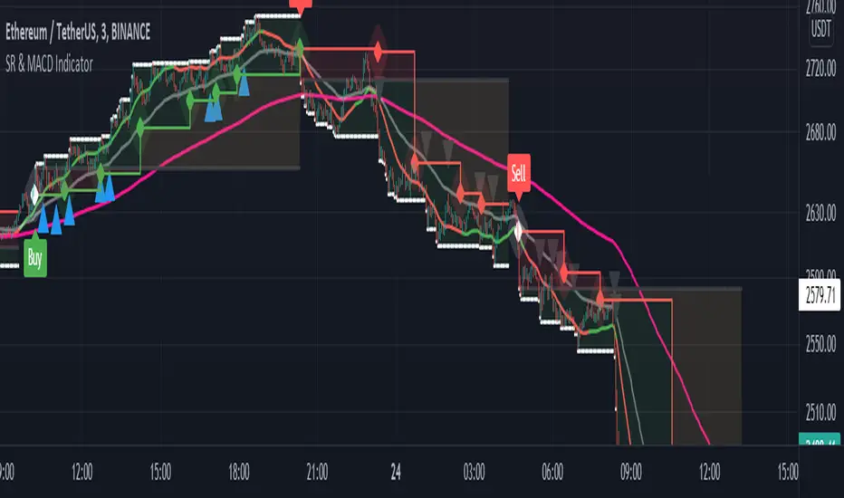
- Primary entry: BLUE/GREEN crosses
- Strong trend confirmation: YELLOW/PURPLE crosses
### Best Practices
1. Trade with the trend (follow RED line direction)
2. Wait for price pullbacks of faster lines
3. Combine crosses with support/resistance levels
4. Use smaller targets
5. Quick exits on failed breakouts
6. Monitor volume for confirmation
### Color Guide
- YELLOW: Fast trend identifier
- BLUE: Very short-term momentum (1min)
- GREEN: Short-term momentum (3min)
- RED: Trend filter
- PURPLE: Strong trend baseline
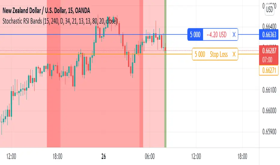
### Risk Management
- Place stops beyond the RED line
- Scale out at key levels
- Use 1:1.5 minimum risk/reward
- Avoid trading during major news
- Reduce position size in choppy markets
### Best Trading Hours
- Most effective during first 2 hours after market open
- Good opportunities during power hour (last hour)
- Avoid lunch hour chop (11:30-1:30 EST)
## Tips
- Less is more - wait for clean setups
- Respect the RED line as your trend filter
- Multiple timeframe confirmation increases success rate
- Use crosses as triggers, not absolute signals
- Practice in simulator before live trading
Indicatore Pine Script®