AMT CVD [hardiman]█ OVERVIEW
AMT CVD is a Cumulative Volume Delta indicator with a unique numeric labeling system designed for the Auction Market Theory (AMT) methodology by Fabio Valentino.
Instead of just showing CVD as a line, this indicator displays numeric labels (+3, +2, +1, 0, -1, -2, -3) and "A" for Absorption, making it easy to identify the current phase of the AMT workflow at a glance.
█ KEY FEATURES
• CVD with numeric aggression labels (+3 to -3)
• "A" label for Absorption detection (high volume + price stagnation)
• Automatic Exhaustion detection (aggression fading)
• Entry signal markers (L for Long, S for Short)
• Real-time workflow dashboard
• Compact Mode for mobile users
• Customizable thresholds and colors
• Built-in alerts for each phase
█ THE NUMERIC LABEL SYSTEM
BUYER AGGRESSION:
• +3 = Extremely aggressive buying (delta > 3.5x average)
• +2 = Strong buying pressure (delta > 2.5x average)
• +1 = Mild buying pressure (delta > 1.5x average)
SELLER AGGRESSION:
• -1 = Mild selling pressure (delta > 1.5x average)
• -2 = Strong selling pressure (delta > 2.5x average)
• -3 = Extremely aggressive selling (delta > 3.5x average)
SPECIAL LABELS:
• 0 = Neutral / Exhaustion (no significant aggression)
• A = Absorption (high volume but price doesn't move)
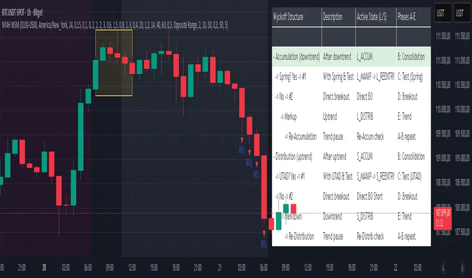
█ AMT WORKFLOW
The indicator tracks the complete AMT entry workflow:
1️⃣ AGGRESSION → Look for +2/+3 or -2/-3 labels
2️⃣ ABSORPTION → Wait for "A" label (price held despite aggression)
3️⃣ EXHAUSTION → Watch labels decrease toward 0
4️⃣ ENTRY → Reversal label appears (direction change)
SHORT SETUP EXAMPLE (at resistance):
+1 → +2 → +3 → A → A → +1 → 0 → -1 → ENTRY SHORT
LONG SETUP EXAMPLE (at support):
-1 → -2 → -3 → A → A → -1 → 0 → +1 → ENTRY LONG
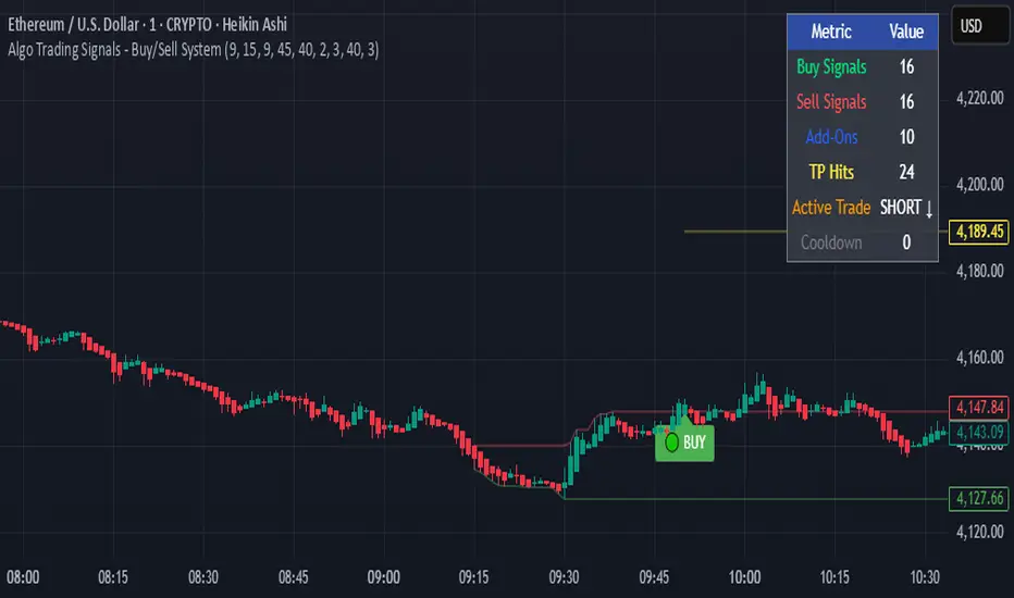
█ DASHBOARD
The dashboard shows real-time status:
• Stage: Current workflow phase (1-5)
• Aggression: Current numeric level
• Absorption: ✓ NOW / ○ RECENT / ✗ NONE
• Exhaustion: ✓ YES / ○ NO
• Signal: WAIT / WATCH / READY / LONG / SHORT
█ HOW TO USE
1. Add this indicator to a separate pane below your chart
2. Use TradingView's built-in SVP HD for key levels (POC/VAH/VAL)
3. Add AMT VWAP for bias determination
4. Wait for price to reach a key level
5. Watch the CVD labels for the AMT sequence
6. Enter when the dashboard shows "READY" or entry signal appears
█ RECOMMENDED SETUP
Complete AMT toolkit:
• Main Chart: SVP HD (built-in) + AMT VWAP
• Lower Pane: AMT CVD (this indicator)
Timeframes:
• Higher TF (H1/H4): Identify structure and key levels
• Entry TF (15m): Execute using this CVD indicator
█ SETTINGS
Display:
• Compact Mode - Simplified view for mobile
• Show Numeric Labels - Toggle the +3/-3 labels
• Label Size - Adjust for your preference
• Dashboard Position - Move to any corner
CVD Settings:
• Relative Length - Period for threshold calculation (default: 20)
• Threshold 1/2/3 - Multipliers for aggression levels
Absorption:
• Volume Multiplier - How much above average = high volume (default: 1.5x)
• Price Threshold - Max price change % for absorption (default: 0.1%)
Colors:
• Fully customizable for buyer/seller/absorption
█ ALERTS
• Absorption Detected - "A" label appears
• Exhaustion Detected - Aggression fading to 0
• Long Entry Signal - Full sequence complete for long
• Short Entry Signal - Full sequence complete for short
█ IMPORTANT NOTES
⚠️ CVD APPROXIMATION: This indicator approximates volume delta from OHLC data. For more accurate CVD, consider using exchange-native order flow tools or Volume Suite by Leviathan as a reference.
⚠️ CONFIRMATION REQUIRED: Signals should be confirmed with:
• Price at key level (VAH/VAL/POC)
• Visual rejection (wicks)
• Higher timeframe bias alignment
█ METHODOLOGY
Based on Auction Market Theory by Fabio Valentino:
"Don't predict, READ the market. Wait for evidence: Aggression → Absorption → Exhaustion → then Execute."
Core principles:
• Location is more important than technique
• Be wrong immediately (tight stops at invalidation)
• Evidence-based entries only
█ CREDITS
Based on Auction Market Theory methodology by Fabio Valentino.
Designed for traders who want a systematic, evidence-based approach.
If this helps your trading, please leave a like! 👍
Questions? Drop a comment below.
```
---
## TAGS (for TradingView)
```
cvd, cumulative-volume-delta, volume-delta, order-flow, auction-market-theory, amt, fabio-valentino, absorption, exhaustion, aggression, entry-signal, day-trading, intraday, volume-analysis, delta
```
---
## CATEGORY
```
Volume
```
Indicatore Pine Script®