Wyckoff Trend Following, Wyckoff Trend Tracking Trading SystemWyckoff Trend Following by Wyckoff Trend Tracking Trading System
Cerca negli script per "track"

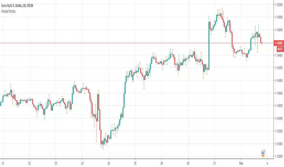
Pivotal Points, Wyckoff Trend Tracking Trading SystemPivotal Points by Wyckoff Trend Tracking Trading System
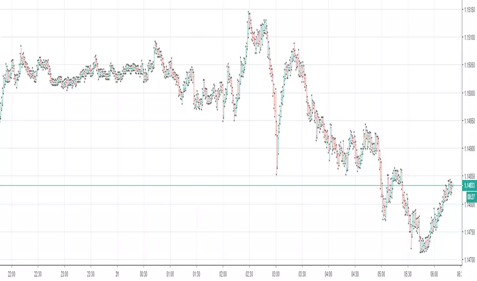
High Volatility Bar, Wyckoff Trend Tracking Trading SystemHigh Volatility Bar by Wyckoff Trend Tracking Trading System

Wyckoff Trend Tracking Momentum IndicatorWyckoff Trend Tracking Momentum Indicator该指标结合量价,让您感受到来自市场的冷热。

Wyckoff Trend Tracking Channel OscillatorWyckoff Trend Tracking Channel Oscillator该指标让您感受到市场传递来的心跳声,随时随地把握市场脉搏。

Wyckoff Trend Tracking Volume TransferWyckoff Trend Tracking Volume Transfer该指标通过对交易量的分析,时刻呈现给您市场的情绪,让您随时感知市场的温度。


Trend Strength Indicator, Wyckoff Trend Tracking Trading SystemTrend Strength Indicator by Wyckoff Trend Tracking Trading System

Wyckoff Trend Following, Wyckoff Trend Tracking Trading SystemWyckoff Trend Following by Wyckoff Trend Tracking Trading System

High Volatility Bar, Wyckoff Trend Tracking Trading SystemHigh Volatility Bar by Wyckoff Trend Tracking Trading System
Pivotal Points, Wyckoff Trend Tracking Trading SystemPivotal Points by Wyckoff Trend Tracking Trading System
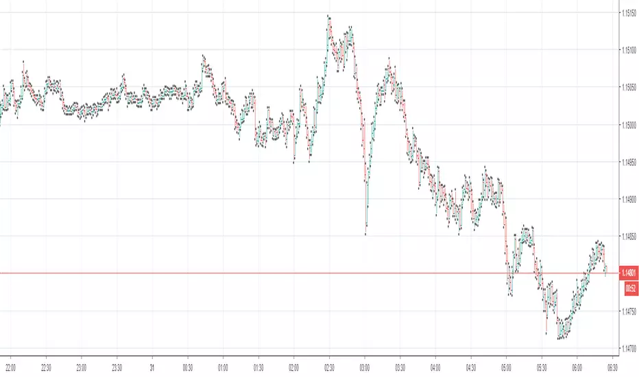
Volume Warning, Wyckoff Trend Tracking Trading SystemVolume Warning by Wyckoff Trend Tracking Trading System
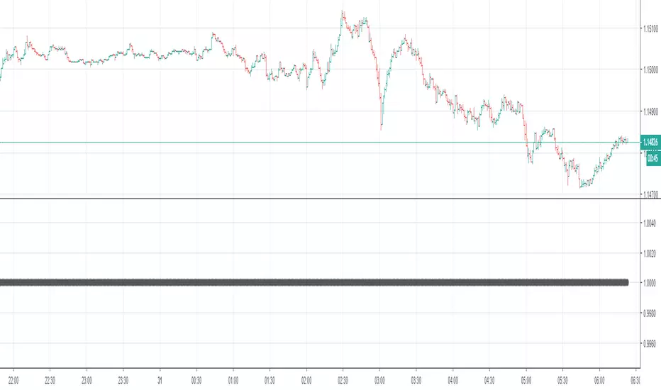
Wyckoff Volume, Wyckoff Trend Tracking Trading SystemWyckoff Volume by Wyckoff Trend Tracking Trading System

Wyckoff Volume on Price, Wyckoff Trend Tracking Trading SystemWyckoff Volume on Price by Wyckoff Trend Tracking Trading System

Wyckoff Trend Tracking Trade SystemWyckoff Trend Tracking Trading System威科夫趋势跟踪交易指标工具为非结构化的市场增添了结构,它有一套明确一致的交易规则,让您专注于具有最高回报和最低风险的交易机会,无论您是刚刚开始从事交易还是经验丰富的交易员,它对您来说绝对是一种竞争优势。


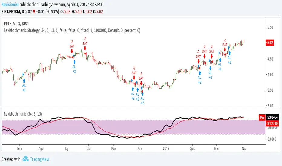
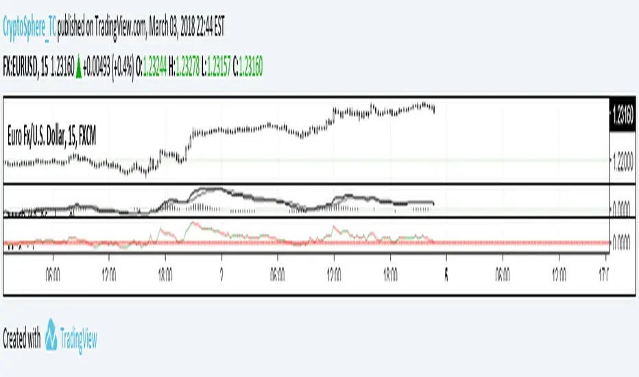
Revistochmanic StrategyRevistochmanic Wave is a stock tracking trends indicator & strategy for medium & long term investing.
Delta price table, BTC Status (track bitcoin price change)If you are trading alt coins which are affected with Bitcoin price movements then this indicator may be useful. It allows you to trade altcoin and track bitcoin price changes simultaneously.
It shows the price change (delta price) for last 60 seconds, 5 minutes, 15 minutes, 30 minutes, 1 hour, 4 hours, 1 day.
If you want any updates, just feel free to write me :)

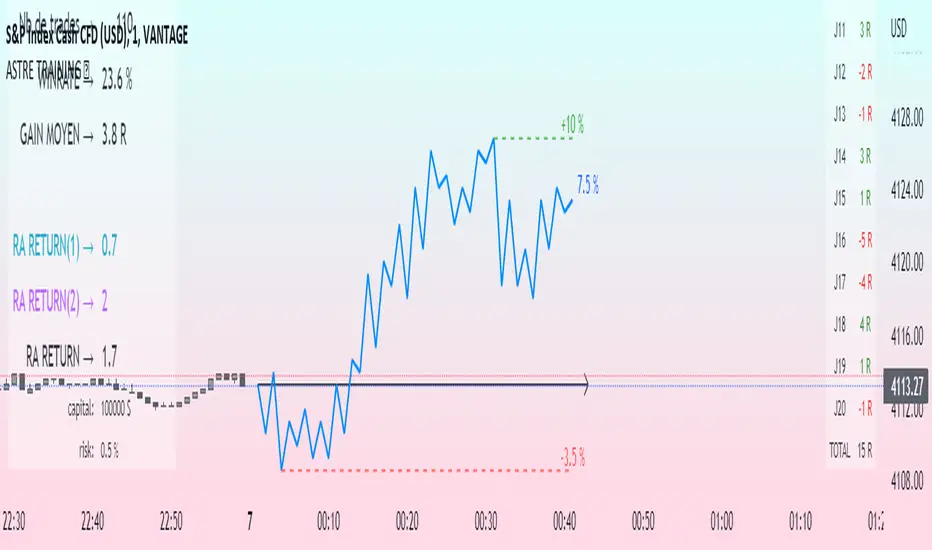
Challenge training (journal)Dynamic trading journal with equity curve display. Detailed results with prop firm objectives, editable, $/month estimation, possibility to compare two strategies.
one line in parameter = one trading day. 20 days max.
For each trading day, specify : The number of trades, the number of SL, the number of total winning RR.
A table at the bottom right summarizes the days and performances during the backtest in order to have an idea of the current performance.
The bottom left table summarizes the overall performance with some key information.
Depending on the number of days traded, a monthly "salary" is deducted, taking into account the prop firm commission.
there is the possibility to define a "Type" for each trading day, 1 or 2. It allows to compare in a binary way, example for type 1: when the high time frame structure is doing well and I am confident for scalping, otherwise type 2.
Again: type 1: SL shorter by 50%, type 2: normal SL etc..
the button "separate 1 and 2" allows to display two additional equity curves : type 1 and type 2. It allows to have a quick visual comparison on the impact of our parameter studied in our backtest on our performance. at the scale of the main equity curve
All the conditions to succeed in the challenge are adjustable in the parameters. The drawdown calculation has been simplified - in order not to have to put 80 trades in the parameters window, I have gathered them by "day", and pessimistically, we consider first the stoplosses and then the take profits, simplifying the performances of the day into "one losing trade" and "one winning trade" (graphically). It is a good compromise between quantity and quality.
Use "A random day trading" indicator to spice up your training.
I hope this will be useful for you to track your performance !
Cyclical TrackThe cyclical track is a simple momentum indicator, created to measuring the speed of prices
Presidential 2020 Candidate and Undecided Voter Poll StatsThis is just a simple indicator to show the election poll stats and include the value for undecided voters.

MACD with Directional ColorsThis MACD indicator colors the MACD and signal lines according to the direction they are moving.
- Eliminates the histogram from the traditional MACD indicator.
- Uses a histogram for the MACD line.
- Includes Bollinger Bands for the MACD line to help detect squeezes
