SIP SmartlyIntroduction:
The SIP Smartly indicator is designed to mimic the behavior of a systematic investment plan, a popular investment strategy where a fixed quantity of an asset is purchased at regular intervals, typically monthly. In this case, we're applying this concept to trading by specifying a start date, a fixed purchase quantity, and certain conditions for buying.
Indicator Components:
User Inputs:
1. Start Date Inputs:
startyear, startmonth, startday: These inputs allow you to specify the year, month, and day when the SIP strategy begins.
2. buyQty:
This input allows you to specify the quantity of the security to purchase in each SIP installment.
What is Standard SIP ?
A Standard Systematic Investment Plan (SIP) is an investment strategy where individuals consistently invest a fixed amount of money at regular intervals, such as monthly or quarterly, in mutual funds or stocks. This approach promotes disciplined and long-term investing, taking advantage of rupee-cost averaging, where more shares are purchased when prices are low and fewer when prices are high. SIPs are designed for individuals seeking gradual wealth accumulation over time while mitigating the impact of market volatility through consistent, automated investments.
Logic of the Smart SIP Indicator:
Dynamic Quantity: The Smart SIP indicator allows you to invest a fixed quantity of a security at regular intervals based on technical analysis conditions. This is different from a standard SIP, where you typically invest a fixed amount of money.
Technical Analysis Driven: The Smart SIP indicator employs technical analysis indicators, such as multiple moving averages and uses the crossover of a higher MA with a lower MA which indicates a possible trend reversal, to determine Buy signals based on price trends. In contrast, a standard SIP doesn't consider technical factors but rather involves regular investments regardless of market conditions.
Adaptability: Unlike a standard SIP, which follows a predetermined investment schedule, the Smart SIP can adapt to changing market conditions. It triggers Buy actions only when specific technical conditions are met, providing a more flexible and responsive approach to investing or trading.
Market Value Tracking: The Smart SIP continuously tracks the market value of the invested quantity in real-time. This allows you to monitor the performance of your SIP investments dynamically, considering market fluctuations. In a standard SIP, you typically track the overall portfolio value without real-time adjustments.
Alert Notifications: The Smart SIP can send alert notifications when Buy conditions are met. This feature ensures timely execution of trades when favorable market conditions align with the technical criteria. In a standard SIP, you usually follow a fixed investment schedule without real-time alerting.
In summary, the unique logic of the Smart SIP indicator lies in its adaptability, technical analysis-driven approach, and real-time tracking and alerting features, making it well-suited for trading in financial markets while still following the concept of a systematic investment plan.
How to Use the SIP Smartly Indicator:
Start Date Selection:
Input your desired start date using the startyear, startmonth, and startday parameters. This is the date when your SIP strategy will begin.
Buy Quantity Setting:
Set the buyQty input to the quantity of the security you want to purchase in each SIP installment.
Alerts:
The indicator can trigger alerts when Buy conditions are met. These alerts can be configured to notify you when it's time to make a SIP installment.
Risk Management and Considerations:
Confirmation: While the SIP Smartly indicator provides insights, use it alongside other technical and fundamental analysis tools for confirmation before making trading decisions.
Backtesting: Before using this indicator in live trading, conduct thorough backtesting on historical data to evaluate its performance under different market conditions.
Position Sizing: Determine your position size and risk management rules based on the quantity purchased in each SIP installment.
Market Awareness: Stay informed about market conditions and news events that could impact price movements. This indicator is a tool to aid your trading strategy, not a standalone solution.
Conclusion:
The SIP Smartly Indicator offers a systematic approach to trading by simulating a SIP strategy. By inputting your start date and desired buy quantity, you can follow a disciplined investment approach in your trading. Remember to customize the inputs to match your trading preferences and risk tolerance.
Disclaimer: This indicator is provided for educational purposes and should be used with caution. Trading involves risks, and you should thoroughly test any strategy before applying it in live trading.
Cerca negli script per "track"

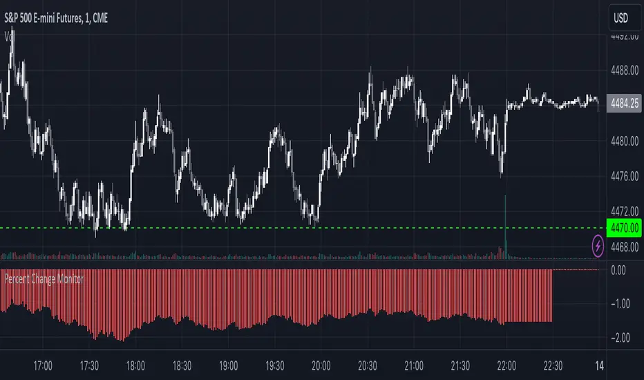
Combined Stock Session Percent Change MonitorIntroducing the "Combined Stock Session Percent Change Monitor" - a unique tool tailored for traders who wish to track the collective performance of up to five stocks in real-time during a trading session.
Key Features:
User Customization: Easily input and monitor any five stock symbols of your choice. By default, the script tracks "AAPL", "MSFT", "AMZN", "TSLA", and "NVDA".
Session-Based Tracking: The script captures and calculates the percentage change from the start of a trading session, set at 15:30. This allows traders to gauge intraday performance.
Visual Clarity: The combined percentage change is plotted as columns, with green indicating a positive change and red indicating a negative change. This provides a clear, visual representation of the stocks' collective performance.
Versatility: Whether you're tracking the performance of stocks in a specific sector, or you're keeping an eye on your personal portfolio's top holdings, this tool offers a concise view of collective stock movement.
Usage:
Simply input the desired stock symbols and let the script do the rest. The plotted columns will provide a quick snapshot of how these stocks are performing collectively since the session's start.
Conclusion:
Stay ahead of the market by monitoring the combined performance of your chosen stocks. Whether you're an intraday trader or a long-term investor, this tool offers valuable insights into collective stock behavior. Happy trading!
(Note: Always conduct your own research and due diligence before making any trading decisions. This tool is meant to aid in analysis and not to serve as financial advice.)
Strategy Developer ToolSolar Strategies: Strategy Developer Tool Complete Guide
This guide provides full explanation of the intended purpose of our script along with individual explanation of each input and the logic behind them coupled with general knowledge which we find useful in using our tool regarding elements of risk and strategy. Use this information wisely and understand we are not providing financial advise, this is a learning tool meant to help advance traders knowledge of the markets and their strategies which are formed as such.
Basics
Before getting into the specifics of how to use our strategy developer tool, it's important to understand a few basic fundamental things about it. The purpose of the tool is to allow the user to optimize a strategy through back testing with our strategy tracker and 50+ user inputs. The way you optimize your strategy depends on a couple things:
The state of the current and recent previous market.
The timeframe you trade on.
The types of trades you prefer. (swings, scalps, etc.)
How much risk you are willing to take on.
Risk Basics:
Going off the last bullet point on the list above, risk plays a huge part in how you optimize your strategy, with that being said here are a few general rules of risk as they relate to trades:
The more trades you take on, the more risk you are opening your strategy up to.
If done correctly, more trades will often result in more profit with slightly lower accuracy, and more risk.
The less trades you take on, the easier it is to have higher accuracy because ideally by rooting out the losing trades, you are left with fewer overall trades but mostly winning trades.
Less trades with higher accuracy often result in less profit but will 100% be less risky than the opposite. (More trades, less accurate, more profit, MORE RISK)
Input Basics:
More trades, less trades, more risk, less risk, what does this all mean as it relates to our tool?
The 50+ user inputs that allow you to optimize and create your strategy all effect when the script takes a trade.
Many of the inputs are essentially conditions. By changing these inputs, what you are doing is changing how specific the conditions need to be in order to take a trade.
This is how the inputs tie into the bullet point list above regarding risk and the number of trades you take on. By raising or lowering certain inputs, you are making the conditions more or less specific on when to trade.
Making conditions more specific will allow for less trades to be taken and will often result in a higher win rate, and less associated risk.
Making conditions less specific will allow for more trades to be taken and depending on the state of the market, could result in more profit being realized, but at the same time opens you up to more risk because you are stating a more general set of conditions in order to take a trade.
How does it work?
Our strategy developer tool is based on two simple factors in order to identify specific areas in the market deemed good for trade. They are as follows:
Directional momentum to identify when a move might happen.
A confirmation of the desired move.
Indicators:
The tool gets its information on these two factors from two custom built indicators which are hard coded into the script. These two indicators and the inputs which affect them can be found labeled with Indicator 1 or Indicator 2 in the tool's settings.
When the conditions are met based on the factors of both indicators, it then decides your stop losses and take profits using pivot points.
Indicator 1 is the momentum indicator.
Indicator 2 looks for confirmation of the move.
Hedges:
Since nothing is ever certain when trading, our tool also aims to minimize potential loss before it can happen by incorporating hedges when a signal prints in the opposite direction of the trade you are currently in.
To identify when to hedge, the candles will appear with the opposite color of your original trade. Candles, while in a long trade, appear as green and candles while in a short trade appear as red. While in a long trade the only time red candles will appear is when a hedge occurs and vice versa for shorts.
Example: If you just took a long trade based on a long signal that the script gave off, but a short signal prints off while you are in the long, you are directed to sell half your long position and enter that half into a short position. Since there is now more uncertainty in the long because of the short signal, minimizing your position size and having a smaller position in the opposite direction allows you to cover your bases if the trade moves against you. If it doesn’t move against you and ends up going long as originally intended, you are not to lose any money, likely a small profit or break even when all is said and done.
In order to give the hedges a greater change of hitting, the take profits are smaller than a normal trade, this way even if your hedge wasn’t necessary and the original trade does not move against you, it's likely that your hedge will still win, and you can just consider it a small scalp to further your profits on the original trade.
Doubles:
Besides minimizing loss, we also aim to maximize the potential gain. When a second signal prints off in the direction of the trade you are currently already in, the tool directs you to double your position size.
The signal for doubling is a label with “2x” written inside.
The logic here is similar to hedging but in the opposite way. Just as a signal in the opposite direction creates uncertainty, a signal in the same direction indicates more certainty hence doubling your position size.
Example: If you are currently in a long position and you get a second long signal, you would then double your existing position since two long signals printing off before the first one has a chance to play out indicates a stronger chance of movement in the intended direction of your trade.
User Inputs
Upon opening the tools settings tab, you will find all the user inputs which can then be modified to fit your desired strategy. In this section of our guides, you will find individual explanations and use cases for each input so you can correctly use them to your best advantage.
Strategy Tracker Table:
By ticking this input on, the strategy tracker table will be visible to the user. (Default is on)
Indicator 1 Greater Than: Long:
By ticking this input on, you are adding a condition the script will then look for in order to take a long. (Default is on)
This condition is that an average of indicator 1, which searches for momentum, must fall above a certain level, which is determined in the next input.
The purpose of this is to ensure that the average momentum is not too low because this would indicate prolonged downwards movement on the timeframe of the market being observed, making a long position riskier.
Indicator 1 Greater Than Input: Long:
This input correlates to the previous input directly above.
If Indicator 1 Greater Than: Long is ticked on, then one of the conditions in order to take a long position will be that the average of indicator 1 must fall above the level which you set in this input.
max level 100, min level 0
Indicator 1 Less Than: Long
By ticking this input on, you are adding a condition the script will then look for in order to take a long position. (Default is on)
This condition is that an average of indicator 1, which searches for momentum, must fall below a certain level, which is determined in the next input.
The purpose of this is to ensure that the average momentum is not too high, because this would indicate a prior significant upwards movement or trend on the timeframe of the market being observed.
Taking a long position while the average momentum is at higher levels exposes the risk of longing as the market has started to pull back from a peak or when the market has just reached a peak.
Indicator 1 Less Than Input: Long
This input correlates to the previous input directly above.
If Indicator 1 Less Than: Long is ticked on, then one of the conditions in order to take a long position will be that the average of indicator 1 must fall below the level which you set in this input.
max level 100, min level 0
Indicator 1 Greater Than: Short
By ticking this input on, you are adding a condition the script will then look for in order to take a short. (Default is on)
This condition is that an average of indicator 1, which searches for momentum, must fall above a certain level, which is determined in the next input.
The purpose of this is to ensure that the average momentum is not too low because this would indicate prolonged downwards movement or trend on the timeframe of the market being observed.
Taking a short position while the average momentum is at lower levels exposes the risk of shorting as the market has started to recover from a bottom or when the market has just reached a bottom.
Indicator 1 Greater Than Input: Short
This input correlates to the previous input directly above.
If Indicator 1 Greater Than: Short is ticked on, then one of the conditions in order to take a short position will be that the average of indicator 1 must fall above the level which you set in this input.
max level 100, min level 0
Indicator 1 Less Than: Short
By ticking this input on, you are adding a condition the script will then look for in order to take a short position. (Default is on)
This condition is that an average of indicator 1, which searches for momentum, must fall below a certain level, which is determined in the next input.
The purpose of this is to ensure that the average momentum is not too high, because this would indicate a prior significant upwards movement or trend on the timeframe of the market being observed.
Taking a short position while the average momentum is at higher levels exposes the risk of shorting as the market is currently in a strong uptrend.
Indicator 1 Less Than: Short
This input correlates to the previous input directly above.
If Indicator 1 Less Than: Short is ticked on, then one of the conditions in order to take a short position will be that the average of indicator 1 must fall below the level which you set in this input.
max level 100, min level 0
Summary of Input Group: Indicator 1 Greater/Less Than Long/Short
This grouping of inputs is best used as a filter of sorts, much like many of the other inputs which are also essentially filters of the market to find areas ripe for trade. Specifically, however, this group of inputs is especially powerful because if used correctly, it can specify a range for the average momentum to fall in when looking for either long or short trades. Think of it like a sweet spot where the average is not too high nor too low. In combination with the numerous other inputs which will shortly be explained, this sweet spot can be a great indication. Keep in mind that once you find a working range, this will not last forever. Conditions in the market are ever changing and as such your inputs, in this case the range the average momentum must fall in, will also need to change with the market conditions.
Bars Since Crossover:
This input simply describes a crossover of the momentum indicator (indicator 1) and its average.
In the category How does it work? Two main factors are discussed, the first being directional momentum to determine when an upwards move might happen. The crossover correlated to this input is the directional momentum as mentioned earlier.
As also mentioned in How does it work? The second factor is a confirmation of the desired upwards move. This confirmation is a crossover of the current price and indicator 2 which will be further addressed later on.
What's important to understand about the two key factors at play in regard to Bars Since Crossover is that this input is determining a condition which looks for a certain number of bars prior to the confirmation of indicator 2 which the crossover of momentum and its average has happened on indicator 1.
Example: Bars Since Crossover input is set to 10. This means that the crossover of momentum and its average from indicator 1 must be within 10 bars prior to the confirmation from indicator 2. If this happens then this condition is met for a long position.
Bars Since Crossunder:
This input simply describes a crossunder of the momentum indicator (indicator 1) and its average.
In the category How does it work? Two main factors are discussed, the first being directional momentum to determine when a downwards move might happen. The crossunder correlated to this input is the directional momentum as mentioned earlier.
As also mentioned in How does it work? The second factor is a confirmation of the desired downwards move. This confirmation is a crossunder of the current price and indicator 2 which will be further addressed later on.
What's important to understand about the two key factors at play in regard to Bars Since Crossunder is that this input is determining a condition which looks for a certain number of bars prior to the confirmation of indicator 2 which the crossunder of momentum and its average has happened on indicator 1.
Example: Bars Since Crossunder input is set to 10. This means that the crossunder of momentum and its average from indicator 1 must be within 10 bars prior to the confirmation from indicator 2. If this happens then this condition is met for a short position.
Summary of Input Group: Bars Since Crossover/Crossunder
These two inputs can have a large effect on the types of trades being taken and the risk which your strategy opens up to. The idea is that in order for the two key factors described in How does it work? to be correlated and therefore indicate a strong directional move, the two events must happen within a somewhat small period of time. If the period of time between the two events taking place is too large, then it's riskier for your strategy due to a delay in directional momentum and the necessary confirmation. It's important to note that this “small period of time” is relative to the security you're trading and the timeframe its being trades on. Small could mean 5 bars in some cases or 20 bars in others, this is why our custom back tester exists. So that the process of optimization on different securities and different timeframes is smooth and only requires adjustments to inputs then your own analysis of the back test results.
Indicator 1 Input Long
Defines how strong the upwards momentum needs to be in order to take a long position.
When optimizing your strategy, this input is likely to have some of the most effect on when the script takes a long position.
The reasoning for this is because the level you set for this input is the level which indicator 1 must close above following the crossover of its average.
Example: Indicator 1 Input Long set to 50, this means that when the momentum crosses over its average from indicator 1, upon the close of this crossover the momentum must be above the level 50 in order for this condition to be met to take a long position.
The higher the level, the stronger the upwards momentum must be, and therefore by using higher levels for this input, the script will search for stronger directional moves leaving less chance for the trade to move against you.
Indicator 1 Input Short
Defines how strong the downwards momentum needs to be in order to take a short position.
When optimizing your strategy, this input is likely to have some of the most effect on when the script takes a short position.
The reasoning for this is because the level you set for this input is the level which indicator 1 must close below following the crossunder of its average.
Example: Indicator 1 Input Short set to 40, this means that when the momentum crosses under its average from indicator 1, upon the close of this crossunder the momentum must be below the level 40 in order for this condition to be met to take a short position.
The lower the level, the stronger the downwards momentum must be, and therefore by using lower levels for this input, the script will search for stronger directional moves leaving less chance for the trade to move against you.
Summary of Input Group: Indicator 1 Input Long/Short
These two inputs are so important to your strategy because at the end of the day no matter how you set it up, it's still a momentum-based strategy. With that being said the level of momentum or the strength needed in order to take trades is of course going to be a key decider in the successfulness of the strategy. When optimizing these two inputs make sure to take into account what the overall market conditions are, meaning if it’s a bull market maybe make the momentum needed to take a long slightly less comparatively to the amount needed to take a short, in other words make long conditions less specific and short conditions more specific. Slight variations of this input can have very big effects, even changing it by 1 or 2 can make a major difference. In might even be good to consider starting optimization with these inputs and then work the rest of the strategy out from there. A lot could be said about these inputs and more docs will be added in order to further explain more strategy approaches revolving around them, for now don’t hesitate to ask any questions.
Indicator 2 Red
This input is used as a sort of chop filter at its base level, however if used correctly it can be a much broader filter for what areas of the market you want to trade in.
Indicator 2 shows as either red or green and is used as a confirmation when price crosses over it following the crossover of momentum and its average from indicator 1 to take a long position.
If ticked on, Indicator 2 Red states a condition in order for the script to take a long position. (Default is on)
The condition is that upon the crossover of the current price and Indicator 2, 10 bars ago indicator 2 must have been red.
The reason for this input is because the current color of indicator 2 upon the crossover must also be red. However, this condition is hard coded in and cannot be changed by any input.
This is because the type of trade being targeted is that of a type of reversal or continuation.
If indicator 2 showed green 10 bars ago and is currently red this would indicate that a top was just reached, and price is reversing downwards making this not a good area to take a long.
Another scenario if indicator 2 showed green 10 bars ago and is currently red is that there is currently a sideways trend going on or otherwise known as chop, also not an ideal area to take a long
However, if 10 bars ago indicator 2 was red and it's currently red this would indicate a more prolonged pullback.
If all conditions are met and we know that price has been pulling back, now we can enter a long with more knowledge pointing to price reversing upwards from a downwards trend, or continuing its upwards trend after a pullback.
Indicator 2 Green
This input is used as a sort of chop filter at its base level, however if used correctly it can be a much broader filter for what areas of the market you want to trade in.
Indicator 2 shows as either red or green and is used as a confirmation when price crosses under it following the crossunder of momentum and its average from indicator 1 to take a short position.
If ticked on, Indicator 2 Green states a condition in order for the script to take a short position. (Default is on)
The condition is that upon the crossunder of the current price and Indicator 2, 10 bars ago indicator 2 must have been green.
The reason for this input is because the current color of indicator 2 upon the crossunder must also be green. However, this condition is hard coded in and cannot be changed by any input.
This is because the type of trade being targeted is that of a type of reversal or continuation.
If indicator 2 showed red 10 bars ago and is currently green this would indicate that a bottom was just reached, and price is reversing upwards making this not a good area to take a short.
Another scenario if indicator 2 showed red 10 bars ago and is currently green is that there is currently a sideways trend going on or otherwise known as chop, also not an ideal area to take a short.
However, if 10 bars ago indicator 2 was green and it's currently green this would indicate a more prolonged upwards movement.
If all conditions are met and we know that price has been moving up, now we can enter a short with more knowledge pointing to price reversing downwards from an upwards trend, or continuing its downwards trend after a bounce up.
Summary of Input Group: Indicator 2 Red/Green
Similar to Indicator 1 Greater/Less Than Long/Short, the goal of these inputs is to try to get a picture of what the previous recent market has been doing. By getting this picture it's easier to find different areas of the market more ideal for trades. Different from Indicator 1 Greater/Less Than Long/Short though, Indicator 2 Red/Green is directly correlated to the price action in the market rather than the momentum. By switching these on or off you are setting more or less specific conditions for taking trades. Some markets require this extra condition to lower your risk in your strategy, however others may not.
Pivot Low
This input is used to define the number of bars the script will look back to grab a pivot low when taking a long position.
This pivot low is then used to set the stop loss when entering a long position.
This input is very important and optimizing it correctly can be extremely crucial to your strategies success.
The Strategy Developer tool uses a 1:1 risk to reward ratio when setting your first take profit point, so when the script looks back to get a pivot low based on the input you set, it will then set your first take profit at an equal ratio to the stop loss found from the pivot low.
The goal in optimizing this input is to give enough lookback to find real pivot points where price has reversed off of, but not to give too much lookback where its grabbing previous pivot points unrelated to the current move of momentum the script is giving a long signal from.
Consider the type of trades you're looking for in your strategy and what timeframe you are trying to trade on.
Longer swing trades which aim to catch bigger moves in the market, possibly on higher time frames, may require a further lookback in order to get your take profits in the correct positioning to catch the desired move, and not exit early before the trade has fully played out.
Shorter scalp trades may aim to catch smaller moves and therefore you don’t want to allow for too much risk by having a large stop loss and large take profits as a result.
Pivot Low 2
Pivot low 2 can be thought of as a backup lookback in order to get the correct pivot low.
In an input which will be discussed shortly called Pivot Low Minimum, you can set a minimum percentage for your pivot low to be, if the pivot low does not meet the minimum then the script will look to Pivot Low 2’s input to use as a bar lookback in order to get the correct pivot low.
This input is used because you might find a Pivot Low input that works well for the majority of the trades in your back tested strategy, however, there will always be outliers and when this Pivot Low input falls short of getting the correct level to put your stop losses at, Pivot Low 2 is used.
Pivot Low 2’s input should always be higher than Pivot Low’s input, that way you can allow the script to look back further in time to find the correct level when the minimum is not met.
Pivot High
This input is used to define the number of bars the script will look back to grab a pivot high when taking a short position.
This pivot high is then used to set the stop loss when entering a short position.
This input is very important and optimizing it correctly can be extremely crucial to your strategies success.
The Strategy Developer tool uses a 1:1 risk to reward ratio when setting your first take profit point, so when the script looks back to get a pivot high based on the input you set, it will then set your first take profit at an equal ratio to the stop loss found from the pivot high.
The goal in optimizing this input is to give enough lookback to find real pivot points where price has reversed off of, but not to give too much lookback where its grabbing previous pivot points unrelated to the current move of momentum the script is giving a short signal from.
Consider the type of trades you're looking for in your strategy and what timeframe you are trying to trade on.
Longer swing trades which aim to catch bigger moves in the market, possibly on higher time frames, may require a further lookback in order to get your take profits in the correct positioning to catch the desired move, and not exit early before the trade has fully played out.
Shorter scalp trades may aim to catch smaller moves and therefore you don’t want to allow for too much risk by having a large stop loss and large take profits as a result.
Pivot High 2
Pivot high 2 can be thought of as a backup lookback in order to get the correct pivot high.
In an input which will be discussed shortly called Pivot High Minimum, you can set a minimum percentage for your pivot high to be, if the pivot high does not meet the minimum then the script will look to Pivot High 2’s input to use as a bar lookback in order to get the correct pivot high.
This input is used because you might find a Pivot High input that works well for the majority of the trades in your back tested strategy, however, there will always be outliers and when this Pivot High input falls short of getting the correct level to put your stop losses at, Pivot High 2 is used.
Pivot High 2’s input should always be higher than Pivot High’s input, that way you can allow the script to look back further in time to find the correct level when the minimum is not met.
Pivot Low Risk Tolerance
This input is very important in managing the risk associated with your strategy.
Pivot Low Risk Tolerance is defining a maximum percentage the pivot low can be away from your entry.
Since the pivot low that’s found is assigned to your stop loss and directly affects the placement of your take profits when taking a long position, making sure the pivot low isn’t too far down is crucial.
Depending on the types of trades you're aiming to take, the timeframe you choose to trade on, and the leverage you use in your strategy, you may want to assign a higher risk tolerance or a lower one.
Example: Pivot Low Risk Tolerance input set to 3, this means that when all other conditions are met in order to take a long position, when searching for the pivot low in order to set a stop loss, if the script finds the pivot low is greater than 3% away from the entry point, it will not take the trade.
Pivot High Risk Tolerance
This input is very important in managing the risk associated with your strategy.
Pivot High Risk Tolerance is defining a maximum percentage the pivot high can be away from your entry.
Since the pivot high that’s found is assigned to your stop loss and directly affects the placement of your take profits when taking a short position, making sure the pivot high isn’t too far up is crucial.
Depending on the types of trades you're aiming to take, the timeframe you choose to trade on, and the leverage you use in your strategy, you may want to assign a higher risk tolerance or a lower one.
Example: Pivot High Risk Tolerance input set to 3, this means that when all other conditions are met in order to take a short position, when searching for the pivot high in order to set a stop loss, if the script finds the pivot high is greater than 3% away from the entry point, it will not take the trade.
Pivot Low Minimum
Sometimes when searching for the pivot low, the script's defined lookback may not be enough to find the proper pivot point.
This can cause improper placement of stop losses and take profits and may cause trades to be exited early before they can fully play out in your favor.
Pivot Low Minimum is an input used to combat this problem, when the script finds a pivot low that does not meet the minimum percentage away from the entry point, it will then turn to Pivot Low 2 input in order to gain a further lookback and grab the correct pivot point to set your stop loss and take profits with.
When reading and setting this input, understand that setting it to 1 means there is no minimum, setting it to 0.9 would mean the minimum is a 10% difference between the pivot low and your entry point.
Think of it in terms of decimals and their equivalent percentage, 0.1 is equal to 10%, 0.01 is equal to 1%.
Whatever percentage you want to set for a minimum, convert it to a decimal, then simply subtract it from 1.
Example: Say you desire a 1.5% minimum pivot low and as a result an equivalent stop loss of 1.5% below your long entry and furthermore a take profit 1.5% above your long entry since the script uses a 1:1 ratio. Converting 1.5% to a decimal would give you 0.015, then subtracting it from 1 would give you 0.985, this would be the input assigned to Pivot Low Minimum.
Pivot High Minimum
Sometimes when searching for the pivot high, the script's defined lookback may not be enough to find the proper pivot point.
This can cause improper placement of stop losses and take profits and may cause trades to be exited early before they can fully play out in your favor.
Pivot High Minimum is an input used to combat this problem, when the script finds a pivot high that does not meet the minimum percentage away from the entry point, it will then turn to Pivot High 2 input in order to gain a further lookback and grab the correct pivot point to set your stop loss and take profits with.
When reading and setting this input, understand that setting it to 1 means there is no minimum, setting it to 0.9 would mean the minimum is a 10% difference between the pivot high and your entry point.
Think of it in terms of decimals and their equivalent percentage, 0.1 is equal to 10%, 0.01 is equal to 1%.
Whatever percentage you want to set for a minimum, convert it to a decimal, then simply subtract it from 1.
Example: Say you desire a 1.5% minimum pivot high and as a result an equivalent stop loss of 1.5% above your short entry and furthermore a take profit 1.5% below your short entry since the script uses a 1:1 ratio. Converting 1.5% to a decimal would give you 0.015, then subtracting it from 1 would give you 0.985, this would be the input assigned to Pivot High Minimum.
Summary of Input Group: Pivot Low/High - Pivot Low/High 2 – Pivot Low/High Risk Tolerance – Pivot Low/High Minimum
The first key takeaway from all these inputs is that your stop losses and take profits will be directly affected through optimizing any of them. The second key takeaway is that these inputs are crucial in managing the risk in your strategy, and while this has been said many times throughout the guide for various inputs, when it comes to stop losses and take profits it is especially true. Having a stop loss which is too high opens up the possibility for much bigger losses, and as a result your take profits will also be too high, minimizing the chance of any of them being hit. Having a stop loss which is too low increases the chance that your trade will get stopped out preemptively, before the trade can mature and move in your favor because remember that trades will not always move immediately in the intended direction, a good amount of patience is often involved in creating consistent successful trades and a successful strategy as such. On the same note, too low of a stop loss could also mean you are missing out on unrealized profit since your take profits are a direct result of the stop loss which is found. When optimizing your pivot low/high risk tolerance, think not about how much you are willing to lose on a single trade, but how much your portfolio can actually afford to lose not just on a single trade but multiple trades, sometimes even in a row. Obviously, the goal in creating a strategy is that you avoid losing trades and especially multiple in a row, however, there are many things that can’t be accounted for. The only way to manage this unaccounted risk is to use proper risk management and not open yourself up to big losses even in the worst most unlikely scenarios. Even if you don’t lose multiple trades in a row, ask yourself, could I afford to lose multiple trades with the risk tolerance I have set if everything were to go to $hit, (hopefully it would not), but in the off chance it did, instead of beating yourself up over what you did wrong, you’ll be patting yourself on the back for what you did right.
TP2-4 Long Placement
The first thing to understand about the take profit placement is that our system of stop losses and take profits uses a 1:1 risk to reward ratio for the first stop loss and first take profit.
This means that if your stop loss falls 2% below your long entry, your first take profit will be 2% above your long entry, hence 1:1.
As for take profits 2-4, they are just extensions of that ratio. This means that if TP2 Long Placement is set to 1.5, the ratio for your second take profit is 1:1.5.
Using the same percentage from the second bullet point being 2%, we can now gather that with a 1:1.5 ratio our second take profit would be at 3% above our long entry.
The same applies for the rest of the take profits, meaning whatever the take profit is set at regardless of which one, apply that number to the second placeholder of the ratio.
Example: First stop loss falls 2% below long entry. TP2 Long Placement input set to 1.5; risk to reward ratio is 1:1.5; corresponding percentage would be a 3% gain. TP3 Long Placement input set to 2; risk to reward ratio is 1:2; corresponding percentage would be a 4% gain. TP4 Long Placement input set to 2.5; risk to reward ratio is 1:2.5; corresponding percentage would be a 5% gain.
The next key thing to understand about the trailing take profits system is the position size being sold at each take profit and therefore how the strategy tracker calculates your strategy's profit.
At the first take profit, 50% of your position is being calculated as sold, locking in good profits off the bat.
At TP2, 20% of your position is being calculated as sold, leaving a remaining 30% open to gain more profit.
At TP3, another 20% of your position is being calculated as sold, leaving 10% to collect any additional possible gains.
At TP4 the remaining 10% of your position is sold and the trade will be fully closed out.
SL2-4 Long Placement
Our system of trailing stop losses is completely similar to that of our trailing take profits.
Just like the trailing take profits, the inputs for stop losses 2-4 are also used as the second placeholders in the risk to reward ratio.
This may be confusing since generally stop losses are associated with a loss on your position, however, the only stop loss which results in a loss on your position is the first one, not stop losses 2-4.
This is because once your first take profit is hit on your long, your stop loss will automatically move up to the price equivalent to the ratio which you set using these inputs that lies in profit.
Example: Since your first take profit will always be at a 1:1 risk to reward ratio with your stop loss, your second take profit could be at a 1:0.8 ratio. So, to clarify, once your first take profit is hit at a 1:1, your original first stop loss will now be moved up in profits to just below your first take profit at a 1:0.8 risk to reward ratio. This only happens AFTER the first take profit is hit.
For stop losses 3 and 4, the same logic is true, once TP2 is hit, your second stop loss will now be moved up to the placement of SL3 which will fall somewhere below TP2. Once TP3 is hit, your third stop loss will now be moved up to the placement of SL4 which will fall somewhere below TP3. If stop loss 4 does not get hit, then the only thing left to happen is for TP4 to hit and the trade will fully close out.
The one major difference between our system of trailing stop losses and take profits is that no matter what stop loss is hit, the entire remainder of your position will be calculated as sold.
So, if your first take profit hits and sells 50% of your long position, but the trade does not continue upwards and moves down to your second stop loss, the remaining 50% of your position will be calculated as sold.
The same applies to SL3 and SL4, so at SL3 the remaining 30% of your position will be calculated as sold, and at SL4 the remaining 10% will be calculated as sold.
Your trailing stop loss placement is dependent on what types of trades you desire. For shorter scalps on smaller timeframes, it's recommended to place each stop loss just below each corresponding take profit for long trades.
This way you leave just enough room for the trade to continue upwards if there is enough momentum, but you don’t open yourself up to losing your unrealized profit if it does not make this continuation.
If you desire longer swing trades on higher timeframes, it might be a good idea to leave more room in between the take profit and corresponding stop loss.
This way you leave more room for the trade to mature and move in your favor since when trading longer moves, often they will not shoot straight up but rather have a series of small pullbacks throughout the more general upwards trend.
Note that when a long trade is first entered the only stop loss and take profit in play are your original stop loss found by the pivot low which would result in a loss, and the first take profit at a 1:1 risk to reward ratio from that pivot low.
TP2-4 Short Placement
The first thing to understand about the take profit placement is that our system of stop losses and take profits uses a 1:1 risk to reward ratio for the first stop loss and first take profit.
This means that if your stop loss falls 2% above your short entry, your first take profit will be 2% below your short entry, hence, 1:1.
As for take profits 2-4, they are just extensions of that ratio. This means that if TP2 Short Placement is set to 1.5, the ratio for your second take profit is 1:1.5.
Using the same percentage from the second bullet point being 2%, we can now gather that with a 1:1.5 ratio our second take profit would be at 3% below our short entry.
The same applies for the rest of the take profits, meaning whatever the take profit is set at regardless of which one, apply that number to the second placeholder of the ratio.
Example: First stop loss falls 2% above short entry. TP2 Short Placement input set to 1.5; risk to reward ratio is 1:1.5; corresponding percentage would be a 3% gain. TP3 Short Placement input set to 2; risk to reward ratio is 1:2; corresponding percentage would be a 4% gain. TP4 Short Placement input set to 2.5; risk to reward ratio is 1:2.5; corresponding percentage would be a 5% gain.
The next key thing to understand about the trailing take profits system is the position size being sold at each take profit and therefore how the strategy tracker calculates your strategy's profit.
At the first take profit, 50% of your position is being calculated as sold, locking in good profits off the bat.
At TP2, 20% of your position is being calculated as sold, leaving a remaining 30% open to gain more profit.
At TP3, another 20% of your position is being calculated as sold, leaving 10% to collect any additional possible gains.
At TP4 the remaining 10% of your position is sold and the trade will be fully closed out.
SL2-4 Short Placement
Our system of trailing stop losses is completely similar to that of our trailing take profits.
Just like the trailing take profits, the inputs for stop losses 2-4 are also used as the second placeholders in the risk to reward ratio.
This may be confusing since generally stop losses are associated with a loss on your position, however, the only stop loss which results in a loss on your position is the first one, not stop losses 2-4.
This is because once your first take profit is hit on your short, your stop loss will automatically move down to the price equivalent to the ratio which you set using these inputs that lies in profit.
Example: Since your first take profit will always be at a 1:1 risk to reward ratio with your stop loss, your second take profit could be at a 1:0.8 ratio. So, to clarify, once your first take profit is hit at a 1:1, your original first stop loss will now be moved down in profits to just below your first take profit at a 1:0.8 risk to reward ratio. This only happens AFTER the first take profit is hit.
For stop losses 3 and 4, the same logic is true, once TP2 is hit, your second stop loss will now be moved down to the placement of SL3 which will fall somewhere above TP2. Once TP3 is hit, your third stop loss will now be moved down to the placement of SL4 which will fall somewhere above TP3. If stop loss 4 does not get hit, then the only thing left to happen is for TP4 to hit and the trade will fully close out.
The one major difference between our system of trailing stop losses and take profits is that no matter what stop loss is hit, the entire remainder of your position will be calculated as sold.
So, if your first take profit hits and sells 50% of your short position, but the trade does not continue downwards and moves up to your second stop loss, the remaining 50% of your position will be calculated as sold.
The same applies to SL3 and SL4, so at SL3 the remaining 30% of your position will be calculated as sold, and at SL4 the remaining 10% will be calculated as sold.
Your trailing stop loss placement is dependent on what types of trades you desire. For shorter scalps on smaller timeframes, it's recommended to place each stop loss just above each corresponding take profit for short trades.
This way you leave just enough room for the trade to continue downwards if there is enough momentum, but you don’t open yourself up to losing your unrealized profit if it does not make this continuation.
If you desire longer swing trades on higher timeframes, it might be a good idea to leave more room in between the take profit and corresponding stop loss.
This way you leave more room for the trade to mature and move in your favor since when trading longer moves, often they will not shoot straight down but rather have a series of small bounces throughout the more general downwards trend.
Note that when a short trade is first entered the only stop loss and take profit in play are your original stop loss found by the pivot high which would result in a loss, and the first take profit at a 1:1 risk to reward ratio from that pivot high.
Summary of Take Profit/Stop Loss Placement:
Correctly placed take profits and stop losses are essential in having a successful strategy and proper risk management. With that being said there are also many ways in which to use this system. Deciding how to set them up is really just a matter of determining the trading style you aim to succeed with. Once this has been determined, the placement of take profits and stop losses should be easier to configure. However, if there is any confusion on either of these topics as the ratios and corresponding TP/SL can get confusing, please do not hesitate to ask further questions in our discord!
Leverage Long
Leverage Long input simply defines the leverage used in your long positions, and is used in calculating the profit in Strategy Tracker
A rundown of risk associated with using leverage will not be given here since it should assume that if you're using leverage, you should already understand the risks.
If you are not using any leverage, then set Leverage Long input to 1.
Long Position Size
This input defines the position size you are using in your long trades.
This input is also used in calculating profit in Strategy Tracker.
Long Hedge Position Size
This input is used to define the position size of long hedge positions.
This input is also used in calculating profit in Strategy Tracker.
Important: Your Long Hedge Position Size should always be half of your Long Position Size for accurate profit calculation.
Double Long Position Size
This input is used to define the position size when in a double long.
This input is also used in calculating profit in Strategy Tracker
Important: Your Double Long Position Size should always be double your Long Position Size for accurate profit calculation.
Short Position Size
This input defines the position size you are using in your short trades.
This input is also used in calculating profit in Strategy Tracker.
Short Hedge Position Size
This input is used to define the position size of short hedge positions.
This input is also used in calculating profit in Strategy Tracker.
Important: Your Short Hedge Position Size should always be half of your Short Position Size for accurate profit calculation.
Double Short Position Size
This input is used to define the position size when in a double short.
This input is also used in calculating profit in Strategy Tracker
Important: Your Double Short Position Size should always be double your Short Position Size for accurate profit calculation.
A Message From the Developer PLEASE READ!!!
If you have made it this far in the guide, I applaud you and thank you for sticking with it as I know there is a lot of information here! This is not an exaggeration when I say there are hundreds of millions of possible variations that could be applied throughout all the inputs which is why I much prefer to call this a tool rather than an algorithm. Algorithm is a loaded word in my opinion as it comes with an implication of guarantee in the trades being made. This is not meant to discourage anybody from taking trades based off the tool which is also why I provided the option for automated alerts which through third party software can turn into automated trades; if you have the confidence in your strategy by all means I encourage you to trade it, automated or not. Just please understand that it's highly recommended to also apply your own knowledge and analysis before taking a trade as historical back testing data has its limitations and cannot always account for current market conditions. The real applicability does not fall in what the back tester window is saying you would have made or how accurate your strategy would have been, it's within the sheer number of markets and scenarios this tool can be used in and the information you can get which a human just can’t comprehend all at once; its literally endless. I urge all of you to be creative and think outside the box about what you can do with such a powerful tool at your fingertips. After all this is the reason why so many inputs were provided. Another main goal of this project was to give users a better understanding of risk management. It can be hard to manage your risk when it’s all kept in your head, but when you can modify your strategy to better manage your risk by simply optimizing a few inputs, it’s a lot easier to comprehend and actually apply when trading. The last thing I want to say is have fun working through the possible learning curve in using this tool, it may be a process but enjoy it because the one thing I can guarantee is that you will come out the other side a better trader than before!

🦍 INSTITUTIONAL DARK POOL & BASKET MANIPULATOR 🚀📝 Indicator Description
🦍 INSTITUTIONAL DARK POOL & BASKET MANIPULATOR 🚀
This is the ultimate edge detection tool for tracking institutional manipulation in basket-linked stocks (e.g., GME, AMC, KOSS). It combines four powerful, independent analysis modules into a single, high-performance indicator. The goal is to identify points of high institutional pressure, coordinated trading, and critical FTD/Gamma Cycle confluence, offering clear BUY/SELL signals and detailed dashboard metrics.
Key Features & Analysis Modules:
🔥 Dark Pool / Unusual Activity Detection: Uses Z-Score analysis on volume spikes, block trade detection, and end-of-day (EOD) institutional sweeps to identify periods of hidden accumulation or distribution. Tracks Cumulative Institutional Pressure to visualize the long-term trend of dark pool activity.
🦍 Basket Correlation Engine: Measures the real-time correlation between the current ticker and up to four user-defined comparison tickers (e.g., meme stocks or related ETFs). Alerts you to a Correlation Break (un-tethering) or a Manipulation Signal (high, synchronized movement) indicative of coordinated basket trading.
📅 T+35 FTD Cycle Tracker: Automatically calculates and highlights the predicted 35-day Failure-to-Deliver (FTD) cycle windows, providing a crucial time-based manipulation context.
⚡ Gamma Pinning Detector: Identifies when the price is being tightly controlled near major option strike prices (e.g., $5, $10, $20), warning of potential Gamma Pinning behavior.
This tool is designed for experienced traders operating on 4-Hour (4H) or Daily timeframes who want to see beneath the surface of the market and exploit institutional footprint.

SMC FVG/IFVG (Multi-TF x 4) [ZAUTEC]SMC FVG/IFVG (Multi-TF x 4): Multi-Timeframe Fair Value Gap with Inversed FVG Detection
This powerful Pine Script indicator is designed to help traders identify, track, and manage Fair Value Gaps (FVGs) and their respective Inversed Fair Value Gaps (IFVGs) across up to four different timeframes simultaneously.
Key Features
Multi-Timeframe Analysis (4x): Analyze and display FVGs from four distinct timeframes alongside your current chart, offering a comprehensive view of market imbalances across various scales.
Fair Value Gap (FVG) Detection: Automatically identifies classic three-candle FVGs (market inefficiencies).
Customizable FVG Length: Set how many bars the FVG boxes should initially extend for.
Minimum Gap Size: Filter out minor, insignificant gaps using a tick-based minimum size threshold.
Optional Box Extension: Dynamically extend FVG boxes to the current bar index or use a fixed extension for a cleaner chart.
Inversed FVG (IFVG) Logic: Detects a high-probability reversal pattern where a previously filled FVG zone is immediately followed by the formation of a new, opposite FVG within or adjacent to the same area. This confirms the old FVG has "flipped roles" (e.g., from support to resistance).
Lookback Period: Defines how long the indicator searches for a corresponding FVG breach to confirm the IFVG.
IFVG Minimum Size: Customizable minimum size threshold for the IFVG.
Dynamic Box Management:
Automatic Fill Deletion: FVGs are automatically removed from the chart when price action fully trades through the gap, signifying the imbalance has been "filled."
IFVG Tracking: IFVGs are tracked and removed from the chart after the configurable lookback period.
Full Customization: Control the visibility, colors, border styles (solid, dashed, dotted), and width for FVG, Bearish FVG, Bullish FVG, and IFVG boxes independently for each of the four timeframes.
How to Use
Select Timeframes: Choose up to four desired timeframes in the settings (e.g., "15" for 15-minute, "4H" for 4-hour, "D" for Daily). Leave the field empty to use the chart's current timeframe.
Toggle Visibility: Use the Show FVG and Show IFVG toggles to focus on the imbalances you wish to see.
Adjust Extension: Set Extend Boxes to bar index to true to keep all open FVG boxes drawn all the way to the current live price bar.
Interpret the Gaps:
FVG (Bullish/Bearish): Potential areas for price to return to and find support/resistance.
IFVG (Inverse FVG): Stronger signals that a previous zone of imbalance has been violated and is likely to act as a significant flip zone for future price movements.
This indicator is an essential tool for traders utilizing concepts like ICT (Inner Circle Trader) and SMC (Smart Money Concepts), providing a clear visual representation of market structure and liquidity voids.

Elite Zone Master Pro - Advanced Multi-Session Trading System🚀 Elite Zone Master Pro - Advanced Multi-Session Trading System
🎯 ORIGINALITY & UNIQUE VALUE PROPOSITION
Elite Zone Master Pro is NOT a simple mashup of existing indicators. It's a proprietary trading system that combines three distinct methodologies into a unified, synergistic approach:
Multi-Session Zone Analysis - Original algorithm for tracking global market sessions
Dynamic Opening Range Breakout (ORB) - Enhanced ORB with bias-aware signal filtering
Advanced Fair Value Gap Detection - Proprietary FVG identification with smart mitigation tracking
🔧 Why This Combination Works
The power lies in how these components work together, not separately:
Session zones provide market context and volatility windows
ORB system identifies key breakout levels during optimal timeframes
FVG detection pinpoints precise entry locations within the ORB framework
Integrated bias system filters signals based on range direction momentum
🧠 DETAILED METHODOLOGY & CALCULATIONS
🌍 1. Multi-Session Zone Framework
What it does: Tracks and visualizes three major global trading sessions simultaneously.
How it works:
Dynamic zone tracking algorithm that calculates session highs/lows in real-time
Adaptive box rendering that expands/contracts based on actual price movement
Session overlap detection for identifying high-volatility periods
Time-weighted zone positioning using custom timezone calculations
Original concepts:
Simultaneous multi-session visualization (not found in standard session indicators)
Dynamic zone expansion based on volatility, not fixed time periods
Cross-session momentum analysis for bias determination
🎯 2. Enhanced Opening Range Breakout System
What it does: Identifies breakout opportunities from predefined session ranges with intelligent bias filtering.
How it works:
Multi-session ORB calculation: Supports US (16:30-16:45), EU (10:00-10:15), Asian (03:00-03:15), and custom sessions
Dynamic range establishment: Range is built in real-time during active session periods
Bias-aware signal filtering: Two-tier breakout system based on range midpoint momentum
Range direction analysis: Compares current range midpoint to previous session's midpoint
Original methodology:
Range Bias Calculation:
- If Current_Midpoint > Previous_Midpoint = Bullish Bias (+1)
- If Current_Midpoint < Previous_Midpoint = Bearish Bias (-1)
- If Current_Midpoint = Previous_Midpoint = Neutral Bias (0)
Signal Logic:
- Bullish Bias: Standard breakout above range high
- Bearish Bias: Enhanced breakout (range_high + 0.5 * range_width) for bullish signals
- Neutral Bias: Standard breakouts both directions
⚡ 3. Advanced Fair Value Gap (FVG) Detection
What it does: Identifies and tracks fair value gaps with automatic mitigation detection.
How it works:
Three-bar gap analysis: Compares current bar relationships to identify true gaps
Dynamic threshold calculation: Auto-adjusting sensitivity based on market volatility
Smart mitigation tracking: Automatically removes filled gaps from display
Directional bias integration: Color-codes gaps based on their directional implication
Proprietary algorithms:
Bullish FVG Criteria:
- Current_Low > High (gap condition)
- Close > High (confirmation)
- (Current_Low - High ) / High > Threshold (significance filter)
Bearish FVG Criteria:
- Current_High < Low (gap condition)
- Close < Low (confirmation)
- (Low - Current_High) / Current_High > Threshold (significance filter)
Mitigation Logic:
- Bullish FVG: Mitigated when Close < FVG_Low
- Bearish FVG: Mitigated when Close > FVG_High
📈 4. Session-Based Moving Average System
What it does: Calculates moving averages that reset and adapt to session boundaries.
How it works:
Session-aware length calculation: Effective length = min(bars_since_session_start, user_length)
Multiple MA types: EMA, SMA, RMA, WMA, VWMA with session-specific calculations
Dynamic smoothing: Adapts to session length for consistent signals across different session durations
🔄 INTEGRATED SYSTEM SYNERGY
🎯 How Components Work Together
Context Layer: Session zones provide market timing context
Setup Layer: ORB system identifies breakout opportunities within optimal timeframes
Entry Layer: FVG detection pinpoints precise entry levels
Filter Layer: Bias system ensures alignment with momentum direction
Confirmation Layer: Session MA provides trend confirmation
🧭 Signal Generation Process
Step 1: Session Analysis
- Identify active trading session
- Calculate session volatility metrics
- Establish range boundaries
Step 2: Range Bias Calculation
- Compare current vs previous range midpoints
- Assign directional bias (-1, 0, +1)
- Adjust breakout thresholds accordingly
Step 3: Breakout Detection
- Monitor price interaction with range boundaries
- Apply bias-specific breakout criteria
- Generate preliminary signals
Step 4: FVG Confirmation
- Scan for fair value gaps within range
- Validate gap significance using dynamic thresholds
- Provide entry refinement opportunities
Step 5: Signal Validation
- Cross-reference with session MA direction
- Ensure alignment with overall bias
- Output final trading signals
📊 PRACTICAL IMPLEMENTATION
🎯 Trading Strategy Framework
Setup Phase:
Configure session times for your timezone
Enable preferred sessions (US/EU/Asian)
Adjust FVG sensitivity based on instrument volatility
Execution Phase:
Wait for range establishment during active session
Monitor for bias-aligned breakouts
Look for FVG retest opportunities
Enter trades with ORB-based stop losses
Risk Management:
Stop loss placement: Outside ORB range boundaries
Position sizing: Based on range width volatility
Trade direction: Must align with calculated range bias
🎨 UNIQUE VISUAL IMPLEMENTATION
📊 Advanced Visualization Features
Multi-layered zone rendering with transparency controls
Dynamic range boxes that adapt to price movement
Smart label positioning to avoid chart clutter
Color-coded bias indication through range fills
Progressive FVG display with automatic cleanup
🔧 TECHNICAL SPECIFICATIONS
⚙️ Performance Optimizations
Efficient array management for FVG tracking
Memory optimization through historical data cleanup
Smart rendering to prevent chart overload
Error handling for edge cases and invalid timeframes
📈 Compatibility
All timeframes under 1 day
All instruments (Forex, Stocks, Crypto, Futures)
All chart types with overlay capability
Mobile and desktop platform support
🏆 WHAT MAKES THIS DIFFERENT FROM OTHER INDICATORS
❌ Standard ORB indicators: Only show basic range breakouts without bias consideration
❌ Basic FVG indicators: Don't integrate with session analysis or range systems
❌ Session indicators: Simply highlight time periods without actionable trading signals
❌ Moving average indicators: Don't adapt to session dynamics
✅ Elite Zone Master Pro: Combines all elements with proprietary logic for a complete trading system
📋 USE CASES & MARKET APPLICATION
🎯 Primary Applications
Forex day trading during major session overlaps
Index futures scalping using session-specific ranges
Cryptocurrency swing trading with 24/7 session analysis
Stock market opening range breakout strategies
📊 Performance Characteristics
Best performance: During high-volatility session transitions
Optimal timeframes: 1m to 4H for intraday trading
Risk-reward ratios: Typically 1:2 to 1:4 based on range width
Win rate: Higher probability when all components align
This indicator represents months of development combining institutional trading concepts with retail accessibility. It's not just another indicator - it's a complete trading methodology in one comprehensive tool.
HTF Fractal Swings [BornKillerBee]Of course. A good description is key to helping other traders understand and use your script. Here are a few options, from a concise version to a more detailed one. You can mix and match parts as you see fit.
Option 1: Concise & To the Point
Title: HTF Fractal Swings
Description:
This indicator automatically identifies and plots significant swing highs (buyside liquidity) and swing lows (sellside liquidity) from a higher timeframe (HTF) directly onto your current chart.
It's designed for traders who use multi-timeframe analysis to map out market structure and identify key areas of interest for entries or targets. Lines extend into the future until price crosses them, providing a clean visual of which liquidity levels are still intact.
Features:
Plots HTF swing points on your lower timeframe chart.
Lines automatically stop extending once liquidity is taken.
Optional "Order Flow Leg" box to visualize the current dealing range between the last major high and low.
Fully customizable: Choose your HTF, number of swings to show, colors, and line styles.
Option 2: Detailed & Feature-Rich (Recommended)
Title: HTF Fractal Swings & Liquidity Visualizer
Description:
Overview
This powerful indicator is designed for price action and smart money concept (SMC) traders who rely on multi-timeframe analysis. It automatically detects Bill Williams' fractal swing points on a user-defined higher timeframe (HTF) and plots them with precision on your current, lower timeframe chart. This allows you to effortlessly track key market structure, identify pools of liquidity, and define the current trading range without ever leaving your chart.
Core Concepts & How to Use
Buyside & Sellside Liquidity: The plotted swing highs represent potential buyside liquidity, which can act as resistance or a target for bullish moves. Conversely, swing lows represent sellside liquidity, acting as potential support or a target for bearish moves.
Dynamic Levels: Lines for each swing level extend into the future, acting as a clear visual guide. When price trades through a level (based on your chosen "Cross Trigger Source"), the line stops extending and its color fades. This provides an instant signal that the liquidity at that price has likely been swept or "taken."
Order Flow Leg: When enabled, the script draws a box connecting the most recent swing high and swing low. This helps visualize the current dealing range or order flow leg. Traders may look for entries at a discount (below 50% of the range) or a premium (above 50%) to target the opposing side of the range.
Key Features
Multi-Timeframe Analysis, Simplified: Define any higher timeframe (e.g., '4H', '1D') and see its key structural points on your '5m' chart.
Precise Swing Placement: The script finds the exact LTF candle responsible for the HTF swing, ensuring the level is plotted with maximum accuracy.
Automatic Liquidity Tracking: Visually confirm when a liquidity level has been breached.
Customizable Display:
Set the number of recent swing highs and lows to track.
Choose whether a cross is triggered by the High/Low (wick) or the bar Close.
Fully control the colors, line styles, and widths for each timeframe.
Toggle the swing time on the labels for historical reference.
This tool is perfect for cleaning up your charts and focusing on the price levels that matter most.

SMC - Institutional Confidence Oscillator [PhenLabs]📊 Institutional Confidence Oscillator
Version: PineScript™v6
📌 Description
The Institutional Confidence Oscillator (ICO) revolutionizes market analysis by automatically detecting and evaluating institutional activity at key support and resistance levels using our own in-house detection system. This sophisticated indicator combines volume analysis, volatility measurements, and mathematical confidence algorithms to provide real-time readings of institutional sentiment and zone strength.
Using our advanced thin liquidity detection, the ICO identifies high-volume, narrow-range bars that signal institutional zone formation, then tracks how these zones perform under market pressure. The result is a dual-wave confidence oscillator that shows traders when institutions are actively defending price levels versus when they’re abandoning positions.
The indicator transforms complex institutional behavior patterns into clear, actionable confidence percentiles, helping traders align with smart money movements and avoid common retail trading pitfalls.
🚀 Points of Innovation
Automated thin liquidity zone detection using volume threshold multipliers and zone size filtering
Dual-sided confidence tracking for both support and resistance levels simultaneously
Sigmoid function processing for enhanced mathematical accuracy in confidence calculations
Real-time institutional defense pattern analysis through complete test cycles
Advanced visual smoothing options with multiple algorithmic methods (EMA, SMA, WMA, ALMA)
Integrated momentum indicators and gradient visualization for enhanced signal clarity
🔧 Core Components
Volume Threshold System: Analyzes volume ratios against baseline averages to identify institutional activity spikes
Zone Detection Algorithm: Automatically identifies thin liquidity zones based on customizable volume and size parameters
Confidence Lifecycle Engine: Tracks institutional defense patterns through complete observation windows
Mathematical Processing Core: Uses sigmoid functions to convert raw market data into normalized confidence percentiles
Visual Enhancement Suite: Provides multiple smoothing methods and customizable display options for optimal chart interpretation
🔥 Key Features
Auto-Detection Technology: Automatically scans for institutional zones without manual intervention, saving analysis time
Dual Confidence Tracking: Simultaneously monitors both support and resistance institutional activity for comprehensive market view
Smart Zone Validation: Evaluates zone strength through volume analysis, adverse excursion measurement, and defense success rates
Customizable Parameters: Extensive input options for volume thresholds, observation windows, and visual preferences
Real-Time Updates: Continuously processes market data to provide current institutional confidence readings
Enhanced Visualization: Features gradient fills, momentum indicators, and information panels for clear signal interpretation
🎨 Visualization
Dual Oscillator Lines: Support confidence (cyan) and resistance confidence (red) plotted as percentage values 0-100%
Gradient Fill Areas: Color-coded regions showing confidence dominance and strength levels
Reference Grid Lines: Horizontal markers at 25%, 50%, and 75% levels for easy interpretation
Information Panel: Real-time display of current confidence percentiles with color-coded dominance indicators
Momentum Indicators: Rate of change visualization for confidence trends
Background Highlights: Extreme confidence level alerts when readings exceed 80%
📖 Usage Guidelines
Auto-Detection Settings
Use Auto-Detection
Default: true
Description: Enables automatic thin liquidity zone identification based on volume and size criteria
Volume Threshold Multiplier
Default: 6.0, Range: 1.0+
Description: Controls sensitivity of volume spike detection for zone identification, higher values require more significant volume increases
Volume MA Length
Default: 15, Range: 1+
Description: Period for volume moving average baseline calculation, affects volume spike sensitivity
Max Zone Height %
Default: 0.5%, Range: 0.05%+
Description: Filters out wide price bars, keeping only thin liquidity zones as percentage of current price
Confidence Logic Settings
Test Observation Window
Default: 20 bars, Range: 2+
Description: Number of bars to monitor zone tests for confidence calculation, longer windows provide more stable readings
Clean Break Threshold
Default: 1.5 ATR, Range: 0.1+
Description: ATR multiple required for zone invalidation, higher values make zones more persistent
Visual Settings
Smoothing Method
Default: EMA, Options: SMA/EMA/WMA/ALMA
Description: Algorithm for signal smoothing, EMA responds faster while SMA provides more stability
Smoothing Length
Default: 5, Range: 1-50
Description: Period for smoothing calculation, higher values create smoother lines with more lag
✅ Best Use Cases
Trending market analysis where institutional zones provide reliable support/resistance levels
Breakout confirmation by validating zone strength before position entry
Divergence analysis when confidence shifts between support and resistance levels
Risk management through identification of high-confidence institutional backing
Market structure analysis for understanding institutional sentiment changes
⚠️ Limitations
Performs best in liquid markets with clear institutional participation
May produce false signals during low-volume or holiday trading periods
Requires sufficient price history for accurate confidence calculations
Confidence readings can fluctuate rapidly during high-impact news events
Manual fallback zones may not reflect actual institutional activity
💡 What Makes This Unique
Automated Detection: First Pine Script indicator to automatically identify thin liquidity zones using sophisticated volume analysis
Dual-Sided Analysis: Simultaneously tracks institutional confidence for both support and resistance levels
Mathematical Precision: Uses sigmoid functions for enhanced accuracy in confidence percentage calculations
Real-Time Processing: Continuously evaluates institutional defense patterns as market conditions change
Visual Innovation: Advanced smoothing options and gradient visualization for superior chart clarity
🔬 How It Works
1. Zone Identification Process:
Scans for high-volume bars that exceed the volume threshold multiplier
Filters bars by maximum zone height percentage to identify thin liquidity conditions
Stores qualified zones with proximity threshold filtering for relevance
2. Confidence Calculation Process:
Monitors price interaction with identified zones during observation windows
Measures volume ratios and adverse excursions during zone tests
Applies sigmoid function processing to normalize raw data into confidence percentiles
3. Real-Time Analysis Process:
Continuously updates confidence readings as new market data becomes available
Tracks institutional defense success rates and zone validation patterns
Provides visual and numerical feedback through the oscillator display
💡 Note:
The ICO works best when combined with traditional technical analysis and proper risk management. Higher confidence readings indicate stronger institutional backing but should be confirmed with price action and volume analysis. Consider using multiple timeframes for comprehensive market structure understanding.
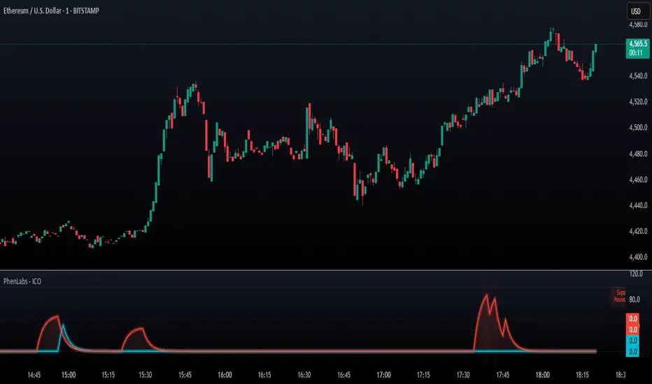
FVG Premium [no1x]█ OVERVIEW
This indicator provides a comprehensive toolkit for identifying, visualizing, and tracking Fair Value Gaps (FVGs) across three distinct timeframes (current chart, a user-defined Medium Timeframe - MTF, and a user-defined High Timeframe - HTF). It is designed to offer traders enhanced insight into FVG dynamics through detailed state monitoring (formation, partial fill, full mitigation, midline touch), extensive visual customization for FVG representation, and a rich alert system for timely notifications on FVG-related events.
█ CONCEPTS
This indicator is built upon the core concept of Fair Value Gaps (FVGs) and their significance in price action analysis, offering a multi-layered approach to their detection and interpretation across different timeframes.
Fair Value Gaps (FVGs)
A Fair Value Gap (FVG), also known as an imbalance, represents a range in price delivery where one side of the market (buying or selling) was more aggressive, leaving an inefficiency or an "imbalance" in the price action. This concept is prominently featured within Smart Money Concepts (SMC) and Inner Circle Trader (ICT) methodologies, where such gaps are often interpreted as footprints left by "smart money" due to rapid, forceful price movements. These methodologies suggest that price may later revisit these FVG zones to rebalance a prior inefficiency or to seek liquidity before continuing its path. These gaps are typically identified by a three-bar pattern:
Bullish FVG : This is a three-candle formation where the second candle shows a strong upward move. The FVG is the space created between the high of the first candle (bottom of FVG) and the low of the third candle (top of FVG). This indicates a strong upward impulsive move.
Bearish FVG : This is a three-candle formation where the second candle shows a strong downward move. The FVG is the space created between the low of the first candle (top of FVG) and the high of the third candle (bottom of FVG). This indicates a strong downward impulsive move.
FVGs are often watched by traders as potential areas where price might return to "rebalance" or find support/resistance.
Multi-Timeframe (MTF) Analysis
The indicator extends FVG detection beyond the current chart's timeframe (Low Timeframe - LTF) to two higher user-defined timeframes: Medium Timeframe (MTF) and High Timeframe (HTF). This allows traders to:
Identify FVGs that might be significant on a broader market structure.
Observe how FVGs from different timeframes align or interact.
Gain a more comprehensive perspective on potential support and resistance zones.
FVG State and Lifecycle Management
The indicator actively tracks the lifecycle of each detected FVG:
Formation : The initial identification of an FVG.
Partial Fill (Entry) : When price enters but does not completely pass through the FVG. The indicator updates the "current" top/bottom of the FVG to reflect the filled portion.
Midline (Equilibrium) Touch : When price touches the 50% level of the FVG.
Full Mitigation : When price completely trades through the FVG, effectively "filling" or "rebalancing" the gap. The indicator records the mitigation time.
This state tracking is crucial for understanding how price interacts with these zones.
FVG Classification (Large FVG)
FVGs can be optionally classified as "Large FVGs" (LV) if their size (top to bottom range) exceeds a user-defined multiple of the Average True Range (ATR) for that FVG's timeframe. This helps distinguish FVGs that are significantly larger relative to recent volatility.
Visual Customization and Information Delivery
A key concept is providing extensive control over how FVGs are displayed. This control is achieved through a centralized set of visual parameters within the indicator, allowing users to configure numerous aspects (colors, line styles, visibility of boxes, midlines, mitigation lines, labels, etc.) for each timeframe. Additionally, an on-chart information panel summarizes the nearest unmitigated bullish and bearish FVG levels for each active timeframe, providing a quick glance at key price points.
█ FEATURES
This indicator offers a rich set of features designed to provide a highly customizable and comprehensive Fair Value Gap (FVG) analysis experience. Users can tailor the FVG detection, visual representation, and alerting mechanisms across three distinct timeframes: the current chart (Low Timeframe - LTF), a user-defined Medium Timeframe (MTF), and a user-defined High Timeframe (HTF).
Multi-Timeframe FVG Detection and Display
The core strength of this indicator lies in its ability to identify and display FVGs from not only the current chart's timeframe (LTF) but also from two higher, user-selectable timeframes (MTF and HTF).
Timeframe Selection: Users can specify the exact MTF (e.g., "60", "240") and HTF (e.g., "D", "W") through dedicated inputs in the "MTF (Medium Timeframe)" and "HTF (High Timeframe)" settings groups. The visibility of FVGs from these higher timeframes can be toggled independently using the "Show MTF FVGs" and "Show HTF FVGs" checkboxes.
Consistent Detection Logic: The FVG detection logic, based on the classic three-bar imbalance pattern detailed in the 'Concepts' section, is applied consistently across all selected timeframes (LTF, MTF, HTF)
Timeframe-Specific Visuals: Each timeframe's FVGs (LTF, MTF, HTF) can be customized with unique colors for bullish/bearish states and their mitigated counterparts. This allows for easy visual differentiation of FVGs originating from different market perspectives.
Comprehensive FVG Visualization Options
The indicator provides extensive control over how FVGs are visually represented on the chart for each timeframe (LTF, MTF, HTF).
FVG Boxes:
Visibility: Main FVG boxes can be shown or hidden per timeframe using the "Show FVG Boxes" (for LTF), "Show Boxes" (for MTF/HTF) inputs.
Color Customization: Colors for bullish, bearish, active, and mitigated FVG boxes (including Large FVGs, if classified) are fully customizable for each timeframe.
Box Extension & Length: FVG boxes can either be extended to the right indefinitely ("Extend Boxes Right") or set to a fixed length in bars ("Short Box Length" or "Box Length" equivalent inputs).
Box Labels: Optional labels can display the FVG's timeframe and fill percentage on the box. These labels are configurable for all timeframes (LTF, MTF, and HTF). Please note: If FVGs are positioned very close to each other on the chart, their respective labels may overlap. This can potentially lead to visual clutter, and it is a known behavior in the current version of the indicator.
Box Borders: Visibility, width, style (solid, dashed, dotted), and color of FVG box borders are customizable per timeframe.
Midlines (Equilibrium/EQ):
Visibility: The 50% level (midline or EQ) of FVGs can be shown or hidden for each timeframe.
Style Customization: Width, style, and color of the midline are customizable per timeframe. The indicator tracks if this midline has been touched by price.
Mitigation Lines:
Visibility: Mitigation lines (representing the FVG's opening level that needs to be breached for full mitigation) can be shown or hidden for each timeframe. If shown, these lines are always extended to the right.
Style Customization: Width, style, and color of the mitigation line are customizable per timeframe.
Mitigation Line Labels: Optional price labels can be displayed on mitigation lines, with a customizable horizontal bar offset for positioning. For optimal label placement, the following horizontal bar offsets are recommended: 4 for LTF, 8 for MTF, and 12 for HTF.
Persistence After Mitigation: Users can choose to keep mitigation lines visible even after an FVG is fully mitigated, with a distinct color for such lines. Importantly, this option is only effective if the general setting 'Hide Fully Mitigated FVGs' is disabled, as otherwise, the entire FVG and its lines will be removed upon mitigation.
FVG State Management and Behavior
The indicator tracks and visually responds to changes in FVG states.
Hide Fully Mitigated FVGs: This option, typically found in the indicator's general settings, allows users to automatically remove all visual elements of an FVG from the chart once price has fully mitigated it. This helps maintain chart clarity by focusing on active FVGs.
Partial Fill Visualization: When price enters an FVG, the indicator offers a dynamic visual representation: the portion of the FVG that has been filled is shown as a "mitigated box" (typically with a distinct color), while the original FVG box shrinks to clearly highlight the remaining, unfilled portion. This two-part display provides an immediate visual cue about how much of the FVG's imbalance has been addressed and what potential remains within the gap.
Visual Filtering by ATR Proximity: To help users focus on the most relevant price action, FVGs can be dynamically hidden if they are located further from the current price than a user-defined multiple of the Average True Range (ATR). This behavior is controlled by the "Filter Band Width (ATR Multiple)" input; setting this to zero disables the filter entirely, ensuring all detected FVGs remain visible regardless of their proximity to price.
Alternative Usage Example: Mitigation Lines as Key Support/Resistance Levels
For traders preferring a minimalist chart focused on key Fair Value Gap (FVG) levels, the indicator's visualization settings can be customized to display only FVG mitigation lines. This approach leverages these lines as potential support and resistance zones, reflecting areas where price might revisit to address imbalances.
To configure this view:
Disable FVG Boxes: Turn off "Show FVG Boxes" (for LTF) or "Show Boxes" (for MTF/HTF) for the desired timeframes.
Hide Midlines: Disable the visibility of the 50% FVG Midlines (Equilibrium/EQ).
Ensure Mitigation Lines are Visible: Keep "Mitigation Lines" enabled.
Retain All Mitigation Lines:
Disable the "Hide Fully Mitigated FVGs" option in the general settings.
Enable the feature to "keep mitigation lines visible even after an FVG is fully mitigated". This ensures lines from all FVGs (active or fully mitigated) remain on the chart, which is only effective if "Hide Fully Mitigated FVGs" is disabled.
This setup offers:
A Decluttered Chart: Focuses solely on the FVG opening levels.
Precise S/R Zones: Treats mitigation lines as specific points for potential price reactions.
Historical Level Analysis: Includes lines from past, fully mitigated FVGs for a comprehensive view of significant price levels.
For enhanced usability with this focused view, consider these optional additions:
The on-chart Information Panel can be activated to display a quick summary of the nearest unmitigated FVG levels.
Mitigation Line Labels can also be activated for clear price level identification. A customizable horizontal bar offset is available for positioning these labels; for example, offsets of 4 for LTF, 8 for MTF, and 12 for HTF can be effective.
FVG Classification (Large FVG)
This feature allows for distinguishing FVGs based on their size relative to market volatility.
Enable Classification: Users can enable "Classify FVG (Large FVG)" to identify FVGs that are significantly larger than average.
ATR-Based Threshold: An FVG is classified as "Large" if its height (price range) is greater than or equal to the Average True Range (ATR) of its timeframe multiplied by a user-defined "Large FVG Threshold (ATR Multiple)". The ATR period for this calculation is also configurable.
Dedicated Colors: Large FVGs (both bullish/bearish and active/mitigated) can be assigned unique colors, making them easily distinguishable on the chart.
Panel Icon: Large FVGs are marked with a special icon in the Info Panel.
Information Panel
An on-chart panel provides a quick summary of the nearest unmitigated FVG levels.
Visibility and Position: The panel can be shown/hidden and positioned in any of the nine standard locations on the chart (e.g., Top Right, Middle Center).
Content: It displays the price levels of the nearest unmitigated bullish and bearish FVGs for LTF, MTF (if active), and HTF (if active). It also indicates if these nearest FVGs are Large FVGs (if classification is enabled) using a selectable icon.
Styling: Text size, border color, header background/text colors, default text color, and "N/A" cell background color are customizable.
Highlighting: Background and text colors for the cells displaying the overall nearest bullish and bearish FVG levels (across all active timeframes) can be customized to draw attention to the most proximate FVG.
Comprehensive Alert System
The indicator offers a granular alert system for various FVG-related events, configurable for each timeframe (LTF, MTF, HTF) independently. Users can enable alerts for:
New FVG Formation: Separate alerts for new bullish and new bearish FVG formations.
FVG Entry/Partial Fill: Separate alerts for price entering a bullish FVG or a bearish FVG.
FVG Full Mitigation: Separate alerts for full mitigation of bullish and bearish FVGs.
FVG Midline (EQ) Touch: Separate alerts for price touching the midline of a bullish or bearish FVG.
Alert messages are detailed, providing information such as the timeframe, FVG type (bull/bear, Large FVG), relevant price levels, and timestamps.
█ NOTES
This section provides additional information regarding the indicator's usage, performance considerations, and potential interactions with the TradingView platform. Understanding these points can help users optimize their experience and troubleshoot effectively.
Performance and Resource Management
Maximum FVGs to Track : The "Max FVGs to Track" input (defaulting to 25) limits the number of FVG objects processed for each category (e.g., LTF Bullish, MTF Bearish). Increasing this value significantly can impact performance due to more objects being iterated over and potentially drawn, especially when multiple timeframes are active.
Drawing Object Limits : To manage performance, this script sets its own internal limits on the number of drawing objects it displays. While it allows for up to approximately 500 lines (max_lines_count=500) and 500 labels (max_labels_count=500), the number of FVG boxes is deliberately restricted to a maximum of 150 (max_boxes_count=150). This specific limit for boxes is a key performance consideration: displaying too many boxes can significantly slow down the indicator, and a very high number is often not essential for analysis. Enabling all visual elements for many FVGs across all three timeframes can cause the indicator to reach these internal limits, especially the stricter box limit
Optimization Strategies : To help you manage performance, reduce visual clutter, and avoid exceeding drawing limits when using this indicator, I recommend the following strategies:
Maintain or Lower FVG Tracking Count: The "Max FVGs to Track" input defaults to 25. I find this value generally sufficient for effective analysis and balanced performance. You can keep this default or consider reducing it further if you experience performance issues or prefer a less dense FVG display.
Utilize Proximity Filtering: I suggest activating the "Filter Band Width (ATR Multiple)" option (found under "General Settings") to display only those FVGs closer to the current price. From my experience, a value of 5 for the ATR multiple often provides a good starting point for balanced performance, but you should feel free to adjust this based on market volatility and your specific trading needs.
Hide Fully Mitigated FVGs: I strongly recommend enabling the "Hide Fully Mitigated FVGs" option. This setting automatically removes all visual elements of an FVG from the chart once it has been fully mitigated by price. Doing so significantly reduces the number of active drawing objects, lessens computational load, and helps maintain chart clarity by focusing only on active, relevant FVGs.
Disable FVG Display for Unused Timeframes: If you are not actively monitoring certain higher timeframes (MTF or HTF) for FVG analysis, I advise disabling their display by unchecking "Show MTF FVGs" or "Show HTF FVGs" respectively. This can provide a significant performance boost.
Simplify Visual Elements: For active FVGs, consider hiding less critical visual elements if they are not essential for your specific analysis. This could include box labels, borders, or even entire FVG boxes if, for example, only the mitigation lines are of interest for a particular timeframe.
Settings Changes and Platform Limits : This indicator is comprehensive and involves numerous calculations and drawings. When multiple settings are changed rapidly in quick succession, it is possible, on occasion, for TradingView to issue a "Runtime error: modify_study_limit_exceeding" or similar. This can cause the indicator to temporarily stop updating or display errors.
Recommended Approach : When adjusting settings, it is advisable to wait a brief moment (a few seconds) after each significant change. This allows the indicator to reprocess and update on the chart before another change is made
Error Recovery : Should such a runtime error occur, making a minor, different adjustment in the settings (e.g., toggling a checkbox off and then on again) and waiting briefly will typically allow the indicator to recover and resume correct operation. This behavior is related to platform limitations when handling complex scripts with many inputs and drawing objects.
Multi-Timeframe (MTF/HTF) Data and Behavior
HTF FVG Confirmation is Essential: : For an FVG from a higher timeframe (MTF or HTF) to be identified and displayed on your current chart (LTF), the three-bar pattern forming the FVG on that higher timeframe must consist of fully closed bars. The indicator does not draw speculative FVGs based on incomplete/forming bars from higher timeframes.
Data Retrieval and LTF Processing: The indicator may use techniques like lookahead = barmerge.lookahead_on for timely data retrieval from higher timeframes. However, the actual detection of an FVG occurs after all its constituent bars on the HTF have closed.
Appearance Timing on LTF (1 LTF Candle Delay): As a natural consequence of this, an FVG that is confirmed on an HTF (i.e., its third bar closes) will typically become visible on your LTF chart one LTF bar after its confirmation on the HTF.
Example: Assume an FVG forms on a 30-minute chart at 15:30 (i.e., with the close of the 30-minute bar that covers the 15:00-15:30 period). If you are monitoring this FVG on a 15-minute chart, the indicator will detect this newly formed 30-minute FVG while processing the data for the 15-minute bar that starts at 15:30 and closes at 15:45. Therefore, the 30-minute FVG will become visible on your 15-minute chart at the earliest by 15:45 (i.e., with the close of that relevant 15-minute LTF candle). This means the HTF FVG is reflected on the LTF chart with a delay equivalent to one LTF candle.
FVG Detection and Display Logic
Fair Value Gaps (FVGs) on the current chart timeframe (LTF) are detected based on barstate.isconfirmed. This means the three-bar pattern must be complete with closed bars before an FVG is identified. This confirmation method prevents FVGs from being prematurely identified on the forming bar.
Alerts
Alert Setup : To receive alerts from this indicator, you must first ensure you have enabled the specific alert conditions you are interested in within the indicator's own settings (see 'Comprehensive Alert System' under the 'FEATURES' section). Once configured, open TradingView's 'Create Alert' dialog. In the 'Condition' tab, select this indicator's name, and crucially, choose the 'Any alert() function call' option from the dropdown list. This setup allows the indicator to trigger alerts based on the precise event conditions you have activated in its settings
Alert Frequency : Alerts are designed to trigger once per bar close (alert.freq_once_per_bar_close) for the specific event.
User Interface (UI) Tips
Settings Group Icons: In the indicator settings menu, timeframe-specific groups are marked with star icons for easier navigation: 🌟 for LTF (Current Chart Timeframe), 🌟🌟 for MTF (Medium Timeframe), and 🌟🌟🌟 for HTF (High Timeframe).
Dependent Inputs: Some input settings are dependent on others being enabled. These dependencies are visually indicated in the settings menu using symbols like "↳" (dependent setting on the next line), "⟷" (mutually exclusive inline options), or "➜" (directly dependent inline option).
Settings Layout Overview: The indicator settings are organized into logical groups for ease of use. Key global display controls – such as toggles for MTF FVGs, HTF FVGs (along with their respective timeframe selectors), and the Information Panel – are conveniently located at the very top within the '⚙️ General Settings' group. This placement allows for quick access to frequently adjusted settings. Other sections provide detailed customization options for each timeframe (LTF, MTF, HTF), specific FVG components, and alert configurations.
█ FOR Pine Script® CODERS
This section provides a high-level overview of the FVG Premium indicator's internal architecture, data flow, and the interaction between its various library components. It is intended for Pine Script™ programmers who wish to understand the indicator's design, potentially extend its functionality, or learn from its structure.
System Architecture and Modular Design
The indicator is architected moduarly, leveraging several custom libraries to separate concerns and enhance code organization and reusability. Each library has a distinct responsibility:
FvgTypes: Serves as the foundational data definition layer. It defines core User-Defined Types (UDTs) like fvgObject (for storing all attributes of an FVG) and drawSettings (for visual configurations), along with enumerations like tfType.
CommonUtils: Provides utility functions for common tasks like mapping user string inputs (e.g., "Dashed" for line style) to their corresponding Pine Script™ constants (e.g., line.style_dashed) and formatting timeframe strings for display.
FvgCalculations: Contains the core logic for FVG detection (both LTF and MTF/HTF via requestMultiTFBarData), FVG classification (Large FVGs based on ATR), and checking FVG interactions with price (mitigation, partial fill).
FvgObject: Implements an object-oriented approach by attaching methods to the fvgObject UDT. These methods manage the entire visual lifecycle of an FVG on the chart, including drawing, updating based on state changes (e.g., mitigation), and deleting drawing objects. It's responsible for applying the visual configurations defined in drawSettings.
FvgPanel: Manages the creation and dynamic updates of the on-chart information panel, which displays key FVG levels.
The main indicator script acts as the orchestrator, initializing these libraries, managing user inputs, processing data flow between libraries, and handling the main event loop (bar updates) for FVG state management and alerts.
Core Data Flow and FVG Lifecycle Management
The general data flow and FVG lifecycle can be summarized as follows:
Input Processing: User inputs from the "Settings" dialog are read by the main indicator script. Visual style inputs (colors, line styles, etc.) are consolidated into a types.drawSettings object (defined in FvgTypes). Other inputs (timeframes, filter settings, alert toggles) control the behavior of different modules. CommonUtils assists in mapping some string inputs to Pine constants.
FVG Detection:
For the current chart timeframe (LTF), FvgCalculations.detectFvg() identifies potential FVGs based on bar patterns.
For MTF/HTF, the main indicator script calls FvgCalculations.requestMultiTFBarData() to fetch necessary bar data from higher timeframes, then FvgCalculations.detectMultiTFFvg() identifies FVGs.
Newly detected FVGs are instantiated as types.fvgObject and stored in arrays within the main script. These objects also undergo classification (e.g., Large FVG) by FvgCalculations.
State Update & Interaction: On each bar, the main indicator script iterates through active FVG objects to manage their state based on price interaction:
Initially, the main script calls FvgCalculations.fvgInteractionCheck() to efficiently determine if the current bar's price might be interacting with a given FVG.
If a potential interaction is flagged, the main script then invokes methods directly on the fvgObject instance (e.g., updateMitigation(), updatePartialFill(), checkMidlineTouch(), which are part of FvgObject).
These fvgObject methods are responsible for the detailed condition checking and the actual modification of the FVG's state. For instance, the updateMitigation() and updatePartialFill() methods internally utilize specific helper functions from FvgCalculations (like checkMitigation() and checkPartialMitigation()) to confirm the precise nature of the interaction before updating the fvgObject’s state fields (such as isMitigated, currentTop, currentBottom, or isMidlineTouched).
Visual Rendering:
The FvgObject.updateDrawings() method is called for each fvgObject. This method is central to drawing management; it creates, updates, or deletes chart drawings (boxes, lines, labels) based on the FVG's current state, its prev_* (previous bar state) fields for optimization, and the visual settings passed via the drawSettings object.
Information Panel Update: The main indicator script determines the nearest FVG levels, populates a panelData object (defined in FvgPanelLib), and calls FvgPanel.updatePanel() to refresh the on-chart display.
Alert Generation: Based on the updated FVG states and user-enabled alert settings, the main indicator script constructs and triggers alerts using Pine Script's alert() function."
Key Design Considerations
UDT-Centric Design: The fvgObject UDT is pivotal, acting as a stateful container for all information related to a single FVG. Most operations revolve around creating, updating, or querying these objects.
State Management: To optimize drawing updates and manage FVG lifecycles, fvgObject instances store their previous bar's state (e.g., prevIsVisible, prevCurrentTop). The FvgObject.updateDrawings() method uses this to determine if a redraw is necessary, minimizing redundant drawing calls.
Settings Object: A drawSettings object is populated once (or when inputs change) and passed to drawing functions. This avoids repeatedly reading numerous input() values on every bar or within loops, improving performance.
Dynamic Arrays for FVG Storage: Arrays are used to store collections of fvgObject instances, allowing for dynamic management (adding new FVGs, iterating for updates).

Active Ranges Detector
1. Purpose
The script identifies and manages bar ranges, which are defined as bars where the high and low prices are fully contained within the high and low of the previous bar. These ranges are used by traders to identify potential breakouts and price consolidations.
2. Key Features
Active Range Validation
A potential range becomes an active range when the price breaks out of the bar’s high or low. The breakout direction is tracked:
• Upward breakout: When the price closes above the high of the range.
• Downward breakout: When the price closes below the low of the range.
The script creates:
• Lines to represent the high and low of the range.
• A colored background box to indicate the range, with color coded for breakout direction:
• Green: Upward breakout.
• Orange: Downward breakout.
Range Updates
• Exit Detection: The script detects if the price exits the range (moves outside the high or low levels).
• Reintegration and Mitigation:
• If the price re-enters an exited range, it marks the range as “mitigated.”
• The lines for mitigated ranges are updated (color and width are changed).
• The background box is removed for mitigated ranges.
3. User Inputs
The script provides customization options:
• Breakout Colors:
• upBreakoutColor: Background color for upward breakout ranges (default: semi-transparent green).
• downBreakoutColor: Background color for downward breakout ranges (default: semi-transparent orange).
• Mitigated Range Styling:
• mitigatedLineColor: Line color for mitigated ranges (default: red).
• mitigatedLineWidth: Width of the line for mitigated ranges.
• Line and Background Settings:
• activeLineWidth: Width of lines for active ranges.
• lineExtension: Length of line extensions beyond the range’s initial boundaries.
• Range Display Limits:
• maxActiveRanges: Maximum number of active ranges to display on the chart (default: up to 200).
4. Visualization
The script provides clear visual feedback for identified ranges:
• Lines: High and low levels of the range are drawn as lines on the chart.
• Background Boxes: Colored boxes are drawn to represent active ranges, with breakout direction indicated by the box’s color.
• Mitigation Styling: Mitigated ranges have updated line styles and no background.
5. Range Management
The script actively manages ranges:
• Tracks the status of each range (active, exited, reintegrated, mitigated).
• Limits the number of displayed ranges to improve chart readability and comply with TradingView’s object limits.
6. Use Case
This script is ideal for traders who:
• Use inside bars to identify areas of consolidation and breakout opportunities.
• Want to track active and mitigated ranges automatically.
• Need a clear, visual representation of ranges and breakout directions.
7. Limitations
• Inside bars are identified based only on the current and previous bar, so the script might not detect more complex consolidation patterns.
• The maximum number of ranges displayed is limited to the user-defined value (maxActiveRanges), with a hard limit of 200 due to TradingView’s object restrictions.

M2 Global Liquidity Index - Time-Shift - KHM2 Global Liquidity Index - Enhanced Time-Shift Indicator
Based on original work by @Mik3Christ3ns3n
Enhanced with advanced time-shift functionality and overlay capabilities.
Description:
This indicator tracks and visualizes the global M2 money supply from five major economies, allowing precise time-shift analysis for correlation studies. All values are converted to USD in real-time and aggregated to provide a comprehensive view of global liquidity conditions.
Key Features:
- Advanced time-shift capability (-1000 to +1000 days) with shape preservation
- Real-time currency conversion to USD
- Overlay functionality with main chart
- Right-scale display for better comparison
- Full historical data preservation during time shifts
Components Tracked:
- US M2 Money Supply (USM2)
- China M2 Money Supply (CNM2)
- Eurozone M2 Money Supply (EUM2)
- Japan M2 Money Supply (JPM2)
- UK M2 Money Supply (GBM2)
Primary Use Cases:
1. Correlation Analysis:
- Compare global liquidity trends with asset prices
- Identify leading/lagging relationships through time-shift
- Study monetary policy impacts across different time periods
2. Market Analysis:
- Track global liquidity conditions
- Monitor central bank policy effects
- Identify potential macro trend changes
Settings:
- Time Offset: Shift the M2 data backwards or forwards (-1000 to +1000 days)
- Positive values: Move M2 data into the future
- Negative values: Move M2 data into the past
- Zero: Current alignment
Technical Notes:
- Data updates follow central banks' M2 publication schedules
- All currency conversions performed in real-time
- Historical shape preservation during time-shifts
- Enhanced data consistency through lookahead mechanism
Credits:
Original concept and base code by @Mik3Christ3ns3n
Enhanced version includes advanced time-shift capabilities and shape preservation
License:
Pine Script™ code is subject to the terms of the Mozilla Public License 2.0
#M2 #GlobalLiquidity #MoneySupply #Macro #CentralBanks #MonetaryPolicy #TimeShift #Correlation #TradingIndicator #MacroAnalysis #LiquidityAnalysis #MarketIndicator

Ticker Tape with Multiple Inputs# Ticker Tape
A customizable multi-symbol price tracker that displays real-time price information in a scrolling ticker format, similar to financial news tickers.
This indicator is inspired from Tradingciew's default tickertape indicator with changes in the way inputs are given.
### Overview
This indicator allows you to monitor up to 15 different symbols simultaneously across any supported exchanges on TradingView. It displays essential price information including current price, price change, and percentage change in an easy-to-read format at the bottom of your chart.
### Features
• Monitor up to 15 different symbols simultaneously
• Support for any exchange available on TradingView
• Real-time price updates
• Color-coded price changes (green for increase, red for decrease)
• Smooth scrolling animation (can be disabled)
• Customizable scroll speed and position offset
### Input Parameters
#### Ticker Tape Controls
• Running: Enable/disable the scrolling animation
• Offset: Adjust the starting position of the ticker tape
#### Symbol Settings
• Exchange (1-15): Enter the exchange name (e.g., NSE, BINANCE, NYSE)
• Symbol (1-15): Enter the symbol name (e.g., BANKNIFTY, RELIANCE, BTCUSDT)
### Display Format
For each symbol, the ticker shows:
1. Symbol Name
2. Current Price
3. Price Change (Absolute and Percentage)
### Example Usage
Input Settings:
Exchange 1: NSE
Symbol 1: BANKNIFTY
Exchange 2: NSE
Symbol 2: RELIANCE
The ticker tape will display:
`NIFTY BANK 46750.00 +350.45 (0.75%) | RELIANCE 2456.85 -12.40 (-0.50%) |`
### Use Cases
1. Multi-Market Monitoring: Track different markets simultaneously without switching between charts
2. Portfolio Tracking: Monitor all your positions in real-time
### Tips for Best Use
1. Group related symbols together for easier monitoring
2. Use the offset parameter to position important symbols in your preferred viewing area
3. Disable scrolling if you prefer a static display
4. Leave exchange field empty for default exchange symbols
### Notes
• Price updates occur in real-time during market hours
• Color coding helps quickly identify price direction
• The indicator adapts to any chart timeframe
• Empty input pairs are automatically skipped
### Performance Considerations
The indicator is optimized for efficiency, but monitoring too many high-frequency symbols might impact chart performance. It's recommended to use only the symbols you actively need to monitor.
Version: 2.0 Stock_Cloud
Last Updated: December 2024
Engulfing BoxThe Engulfing Box indicator is a custom script designed to visually highlight and track bullish and bearish engulfing candlestick patterns on a price chart. These patterns are often used to identify potential reversal points, making them valuable for technical analysis. The script dynamically draws colored boxes around these patterns, helping users easily spot them in the price action.
Key Features:
Bullish Engulfing Pattern: When a candlestick fully engulfs the previous bearish candle (i.e., the close of the current candle is higher than the open of the previous candle, and the open is lower than the close of the previous candle), the script draws a green box around the bullish engulfing candle. This box is drawn from the open of the previous candle to the low of the previous candle.
Bearish Engulfing Pattern: When a candlestick fully engulfs the previous bullish candle (i.e., the close of the current candle is lower than the open of the previous candle, and the open is higher than the close of the previous candle), a red box is drawn around the bearish engulfing candle. This box is drawn from the open of the previous candle to the high of the previous candle.
Dynamic Box Management: Once an engulfing pattern is detected, a box is drawn with the following attributes:
Bullish Engulfing Box: Green, with a transparent background.
Bearish Engulfing Box: Red, with a transparent background.
The box will adjust its color to gray if the price moves past certain thresholds, indicating that the engulfing pattern may no longer be as relevant.
Max Pattern Tracking: The script limits the number of engulfing boxes tracked on the chart to prevent clutter. The maximum number of bullish and bearish engulfing patterns shown is customizable (set to 500 by default), and once this limit is exceeded, older boxes are deleted to maintain a clean chart.
Pattern Expiry: Boxes are deleted if price action moves beyond the pattern’s range, ensuring that outdated signals are removed. If the low price falls below the bottom of the bullish engulfing box, or the high price rises above the top of the bearish engulfing box, the respective box is removed. Additionally, if the low price moves below the top of the bullish box or the high price exceeds the bottom of the bearish box, the box's color is changed to a more neutral tone.
How it Works:
Pattern Detection: The script compares the current price data with the previous candlestick to detect the bullish or bearish engulfing patterns.
Box Creation: If a pattern is detected, a colored box is drawn around the candle to visually highlight the pattern.
Pattern Expiry and Cleanup: The script continuously monitors past boxes. If the price moves too far from the box’s range, the box is either deleted or altered to reflect the reduced significance of the pattern.
B ox Count Limit: To avoid clutter, the script ensures that no more than 500 bullish or bearish engulfing boxes are shown at any time.
Customization:
The number of previous bars to scan for engulfing patterns can be adjusted (maxBarsback).
The maximum number of patterns displayed at any time can be modified.

Edufx's Power of ThreeIndicator Overview
Name: Edufx's Power of Three
Purpose:
To highlight the high and low price ranges of specific hourly candles on a chart.
To visualize these ranges using rectangles.
Features
Visibility Toggle:
Users can enable or disable the visibility of the rectangles highlighting the high and low price ranges of the specified candles.
Customizable Rectangle Length:
Users can adjust the length of the rectangles that extend from the specified candle's high and low prices.
Price Range Tracking:
The high and low prices of the specified candles are tracked and stored.
Rectangle Drawing:
Rectangles are drawn from 5 bars before the end of the specified hour, highlighting the high and low price ranges.
How It Works
Price Range Tracking:
During each specified hour, the high and low prices are updated with the highest and lowest prices observed.
Rectangle Drawing:
At the end of each specified hour, the high and low prices are used to draw rectangles extending 5 bars backward from the end of the hour.
Rectangles are color-coded (red, green, and blue) for easy identification.
Usage
This indicator is useful for traders who want to monitor and react to key price levels at specific times of the day.
The visual rectangles help in identifying potential trading opportunities based on price action relative to these key levels.
Example
If the price moves above the high of the specified candle but fails to close above it, a visual rectangle will highlight this price range.
Similarly, if the price moves below the low of the specified candle but fails to close below it, the rectangle will indicate this range.
This indicator provides visual aids to assist traders in making informed decisions based on the behavior of price at specific key levels.

Market Internals & InfoThis script provides various information on Market Internals and other related info. It was a part of the Daily Levels script but that script was getting very large so I decided to separate this piece of it into its own indicator. I plan on adding some additional features in the near future so stay tuned for those!
The script provides customizability to show certain market internals, tickers, and even Market Profile TPO periods.
Here is a summary of each setting:
NASDAQ and NYSE Breadth Ratio
- Ratio between Up Volume and Down Volume for NASDAQ and NYSE markets. This can help inform about the type of volume flowing in and out of these exchanges.
Advance/Decline Line (ADL)
The ADL focuses specifically on the number of advancing and declining stocks within an index, without considering their trading volume.
Here's how the ADL works:
It tracks the daily difference between the number of stocks that are up in price (advancing) and the number of stocks that are down in price (declining) within a particular index.
The ADL is a cumulative measure, meaning each day's difference is added to the previous day's total.
If there are more advancing stocks, the ADL goes up.
If there are more declining stocks, the ADL goes down.
By analyzing the ADL, investors can get a sense of how many stocks are participating in a market move.
Here's what the ADL can tell you:
Confirmation of Trends: When the ADL moves in the same direction as the underlying index (e.g., ADL rising with a rising index), it suggests broad participation in the trend and potentially stronger momentum.
Divergence: If the ADL diverges from the index (e.g., ADL falling while the index is rising), it can be a warning sign. This suggests that fewer stocks are participating in the rally, which could indicate a weakening trend.
Keep in mind:
The ADL is a backward-looking indicator, reflecting past market activity.
It's often used in conjunction with other technical indicators for a more complete picture.
TRIN Arms Index
The TRIN index, also called the Arms Index or Short-Term Trading Index, is a technical analysis tool used in the stock market to gauge market breadth and sentiment. It essentially compares the number of advancing stocks (gaining in price) to declining stocks (losing price) along with their trading volume.
Here's how to interpret the TRIN:
High TRIN (above 1.0): This indicates a weak market where declining stocks and their volume are dominating the market. It can be a sign of a potential downward trend.
Low TRIN (below 1.0): This suggests a strong market where advancing stocks and their volume are in control. It can be a sign of a potential upward trend.
TRIN around 1.0: This represents a more balanced market, where it's difficult to say which direction the market might be headed.
Important points to remember about TRIN:
It's a short-term indicator, primarily used for intraday trading decisions.
It should be used in conjunction with other technical indicators for a more comprehensive market analysis. High or low TRIN readings don't guarantee future price movements.
VIX/VXN
VIX and VXN are both indexes created by the Chicago Board Options Exchange (CBOE) to measure market volatility. They differ based on the underlying index they track:
VIX (Cboe Volatility Index): This is the more well-known index and is considered the "fear gauge" of the stock market. It reflects the market's expectation of volatility in the S&P 500 index over the next 30 days.
VXN (Cboe Nasdaq Volatility Index): This is a counterpart to the VIX, but instead gauges volatility expectations for the Nasdaq 100 index over the coming 30 days. The tech-heavy Nasdaq can sometimes diverge from the broader market represented by the S&P 500, hence the need for a separate volatility measure.
Both VIX and VXN are calculated based on the implied volatilities of options contracts listed on their respective indexes. Here's a general interpretation:
High VIX/VXN: Indicates a high level of fear or uncertainty in the market, suggesting investors expect significant price fluctuations in the near future.
Low VIX/VXN: Suggests a more complacent market with lower expectations of volatility.
Important points to remember about VIX and VXN:
They are forward-looking indicators, reflecting market sentiment about future volatility, not necessarily current market conditions.
High VIX/VXN readings don't guarantee a market crash, and low readings don't guarantee smooth sailing.
These indexes are often used by investors to make decisions about portfolio allocation and hedging strategies.
Inside/Outside Day
This provides a quick indication of it we are still trading inside or outside of yesterdays range and will show "Inside Day" or "Outside Day" based upon todays range vs. yesterday's range.
Custom Ticker Choices
Ability to add up to 5 other tickers that can be tracked within the table
Show Market Profile TPO
This only shows on timeframes less than 30m. It will show both the current TPO period and the remaining time within that period.
Table Customization
Provided drop downs to change the text size and also the location of the table.

TradeTrackerv2Library "TradeTrackerv2"
This library can be used to track (hypothetical) trades on the chart. Enter the Open, SL, and TP prices (or TP in R to have it calculated) and then call Trade.TrackTrade(barIndex). Keep track of your trades in an array and then simply call TradeTracker.UpdateAllTrades(close) to update all trades based on the current close price.
How to use:
1. Import the library, as always. I'm assuming the alias of "Tracker" below.
2. The Type Trade is exported, so generate a Trade object like newTrade = Tracker.Trade.new() .
3. Set the values for Open, SL, and TP. TP can be set either by price or by R, which will calculate the R based on the Open->SL range:
newTrade.priceOpen = 1.0
newTrade.priceSl = 0.5
newTrade.priceTp = 2.0
-- or in place of the third line above --
newTrade.rTp = 2
4. On each interval you want to update (whether that's per tick/close or on each bar), call trades.UpdateAllTrades(close) . This snippet assumes you have an array named trades (var trades = array.new()) .
In future updates, more customization options will be created. This is the initial prototype.
method MakeTradeLines(t, barIdx)
Namespace types: Trade
Parameters:
t (Trade)
barIdx (int)
method UpdateLabel(t)
Namespace types: Trade
Parameters:
t (Trade)
method MakeLabel(t, barIdx)
Namespace types: Trade
Parameters:
t (Trade)
barIdx (int)
method CloseTrade(t)
Namespace types: Trade
Parameters:
t (Trade)
method OpenTrade(t)
Namespace types: Trade
Parameters:
t (Trade)
method OpenCloseTrade(t, _close)
Namespace types: Trade
Parameters:
t (Trade)
_close (float)
method CalculateProfits(t, _close)
Calculates profits/losses for the Trade, given _close price
Namespace types: Trade
Parameters:
t (Trade)
_close (float)
method UpdateTrade(t, _close)
Namespace types: Trade
Parameters:
t (Trade)
_close (float)
method SetInitialValues(t, barIdx)
Namespace types: Trade
Parameters:
t (Trade)
barIdx (int)
method UpdateAllTrades(trades, _close)
Namespace types: Trade
Parameters:
trades (Trade )
_close (float)
method TrackTrade(t, barIdx)
Namespace types: Trade
Parameters:
t (Trade)
barIdx (int)
Trade
Fields:
id (series__integer)
isOpen (series__bool)
isClosed (series__bool)
isBuy (series__bool)
priceOpen (series__float)
priceTp (series__float)
priceSl (series__float)
rTP (series__float)
profit (series__float)
r (series__float)
resultR (series__float)
lineOpen (series__line)
lineTp (series__line)
lineSl (series__line)
labelStats (series__label)
World Markets Table
🌍 World Markets Session Table - Track Global Exchanges in Real-Time
Monitor 10 major stock exchanges worldwide with live market status, countdown timers, and customizable themes. Perfect for multi-market traders, global portfolio managers, and anyone trading across time zones.
✨ Key Features
10 Global Exchanges Tracked:
🇺🇸 NYSE & NASDAQ (New York)
🇨🇳 Shanghai Stock Exchange
🇯🇵 Tokyo Stock Exchange
🇭🇰 Hong Kong Stock Exchange
🇬🇧 London Stock Exchange
🇪🇺 Euronext
🇩🇪 Frankfurt (Xetra)
🇨🇦 Toronto Stock Exchange
🇦🇺 Australian Securities Exchange
Real-Time Market Intelligence:
✅ Live OPEN/CLOSED status with colored indicators
⏱️ Countdown timers to market open/close
🗓️ Automatic weekday/weekend detection
🕒 Optional seconds display for precision timing
🎯 Visual status badges (green for open, red for closed)
Full Customization:
📍 6 table positions (top/bottom × left/center/right)
📏 4 size options (tiny, small, normal, large)
🎨 4 professional themes: Dark, Light, Neon, Ocean
🚩 Toggle country flags on/off
💼 Clean, professional table layout
🎨 Professional Themes
Dark Theme: Sleek charcoal design for night trading
Light Theme: Bright, clean interface for daylight charts
Neon Theme: Vibrant cyberpunk aesthetic with electric colors
Ocean Theme: Calming blue palette for focused analysis
💡 Perfect For
Multi-market traders monitoring global sessions simultaneously
Identifying optimal trading windows across time zones
Planning entries/exits around market opens and closes
Portfolio managers tracking international markets
Forex, indices, and commodities traders
Pre-market and after-hours trading planning
⚙️ How It Works
All market times are calculated in UTC and automatically adjust to your local timezone. The indicator overlays your chart without interfering with price action or technical analysis. Simply add it to any chart, customize the appearance, and stay informed about global market hours.
📊 Usage Tips
Place the table in a non-intrusive position to maintain chart clarity
Use countdown timers to prepare for volatility at market open/close
Match the theme to your chart colors for a cohesive workspace
Enable seconds display when precision timing matters most
Note: This is a display-only indicator showing market hours. It does not generate trading signals or plot price data.
Premarket LevelsThis indicator tracks premarket high and low levels for day trading, providing statistical analysis on how often these levels get touched during regular trading hours (9:30 AM-4:00 PM EST). It combines real-time level tracking with historical probability analysis and precise timing statistics to help traders make data-driven decisions. I use 4:00 - 9:30 AM on SPY/QQQ etc and 18:00 - 9:30 on Futures ES/NQ etc
Core Features
1. Premarket Level Tracking
Automatically identifies and plots premarket high and low levels
Displays levels with customizable colors and line styles
Shows optional midpoint and percentage/fibonacci retracement levels
Tracks when levels are set during premarket session
2. Historical Touch Analysis
Calculates probability of PM high/low being touched during regular hours
Tracks "Both Levels" touched rate (how often both get hit same day)
Tracks "Either Level" touched rate (how often at least one gets hit)
Adjustable lookback period (1-250 days) for statistical analysis
3. Timing Intelligence
Average time when levels get touched
Earliest and latest touch times in historical data
Four customizable time buckets showing touch distribution throughout the day
First touch time displayed for current session
4. Range Analysis
Current PM range vs historical average (adjustable period)
Range percentile ranking (where today ranks in historical distribution)
Min/Max historical ranges for context
Large/small range detection with customizable thresholds
Background highlighting for unusual range days
5. Smart Signals & Alerts
Buy/Sell signals on level breakouts (adjustable sensitivity)
Level rejection detection (failed breakout patterns)
Proximity alerts when approaching levels
Touch markers (diamond shapes) when levels are tested
Multiple alert conditions for various scenarios
6. Risk Management Tools
Automatic stop loss suggestions (ATR-based, percentage-based, or fixed points)
Target projections based on range extension
Position tracking relative to PM range
Distance calculations to both levels
How To Use
For Day Traders:
Check the "Either Level" percentage - if 90%+, at least one level will likely be touched
Review time bucket statistics - most touches happen 9:30-10:00 AM
Monitor "Both Levels" rate - typically only 20-30%, meaning round trips are rare
Use range percentile to gauge if expansion or mean reversion is likely
For Scalpers:
Enable touch markers to see exact level tests
Use proximity alerts to prepare for potential bounces
Monitor first touch times - early touches often lead to continuations
Check rejection signals for quick reversal trades
For Swing Position Sizing:
Use historical touch rates to assess probability of level tests
Review range size vs average for stop placement guidance
Check timing analysis to avoid holding through low-probability windows
Use target projections for realistic profit targets
Settings Overview
Basic Settings:
Premarket session time (default 4:00-7:30 AM EST)
Signal sensitivity for breakout detection
Timezone selection for accurate time labels
Historical Analysis:
Lookback period for statistics (default 20 days, max 250)
Toggle touch tracking and markers
Enable/disable daily statistics display
Range Analysis:
Adjustable average period (default 20 days)
Large/small range threshold customization
Range percentile display toggle
Timing Analysis:
Three customizable time buckets (default: 10:00, 11:00, 12:00)
Fourth bucket automatically covers afternoon (12:00-4:00 PM)
Toggle time bucket statistics display
Visual Features:
Midpoint line display
Percentage (25%, 75%) or Fibonacci (23.6%, 38.2%, 61.8%, 78.6%) levels
Table position and size customization
Comprehensive color scheme customization (background, text, headers)
Smart Alerts:
Proximity alerts with adjustable threshold
Level rejection detection
Failed breakout detector
Time-of-day filter to avoid lunch chop
Risk Management:
Stop loss method selection (ATR, PM Range %, Fixed Points)
Adjustable ATR multiplier
Target projection display
Statistics Explained
Touch Rates:
Percentage of days where level was touched during RTH
Based only on FIRST touch per day (not multiple re-tests)
Binary metric: Yes/No for each day
Timing Stats:
All based on timestamp of FIRST touch each day
Average, Earliest, Latest provide distribution context
Time buckets show concentration of first touches
Range Metrics:
Current range compared to historical average
Percentile shows where today ranks (0-100%)
Min/Max provide extreme boundaries from history
Important Notes
First Touch Only: All statistics track only the first time a level is touched each day, not subsequent re-tests
RTH Focus: Touch tracking occurs only during regular trading hours (9:30 AM-4:00 PM EST)
Data Accumulation: Historical statistics build over time as indicator runs; requires specified lookback period to populate
Chart Timeframe: Works on any timeframe but recommended 3-5 minute charts for best premarket level precision
Memory Reset: Each new premarket session resets tracking for fresh daily analysis
Best Practices
Use 60-100 day lookback for statistical significance
Combine high touch rates (80%+) with time bucket data for highest probability setups
Small ranges (< 50% of average) often lead to expansion moves
Large ranges (> 150% of average) often consolidate or mean-revert
First 30 minutes typically contains 50%+ of all level touches
After 12:00 PM, probability of untouched levels being hit drops significantly
Performance Considerations
Optimized for real-time calculation with minimal lag
Uses efficient array management for historical data
Table updates only on bar close for performance
Maximum lookback of 250 days to prevent memory issues
This indicator is for educational and informational purposes only. It is NOT financial advice.
The buy/sell signals are algorithmic suggestions based on historical patterns and should NOT be followed blindly
Past performance and historical statistics do NOT guarantee future results
All trading involves substantial risk of loss
You are solely responsible for your own trading decisions
Always perform your own analysis and risk assessment before entering any trade
The creator of this indicator is not responsible for any trading losses incurred from its use
No representation is being made that any account will or is likely to achieve profits or losses similar to those discussed in the indicator statistics
By using this indicator, you acknowledge that you understand these risks and accept full responsibility for your trading decisions.

PIPSTA - ORB# PIPSTA - ORB - Complete Explanation
This is a sophisticated **Opening Range Breakout (ORB)** indicator for TradingView that tracks price movements during the first minutes of a trading session and identifies breakout opportunities.
---
## 🎯 Core Concept: What is ORB?
**Opening Range Breakout** is a trading strategy based on the idea that the first minutes of trading establish key support/resistance levels. When price breaks above (bullish) or below (bearish) these levels with conviction, it often signals a strong directional move for the rest of the session.
---
## 📊 Key Features
### 1. **Multi-Stage ORB Tracking**
The indicator tracks **4 different opening ranges simultaneously**:
- **ORB 5**: First 5 minutes (fastest, most volatile)
- **ORB 15**: First 15 minutes (balanced signals)
- **ORB 30**: First 30 minutes (more reliable)
- **ORB 60**: First 60 minutes (slowest, most confirmed)
Each stage establishes a **High** and **Low** level. The active ORB (usually the largest completed one) is used for breakout detection.
---
### 2. **Breakout Detection System**
**How it works:**
- Monitors when price closes **above ORB High** (bullish breakout) or **below ORB Low** (bearish breakout)
- Requires a **buffer** (default 0.2%) to filter false breakouts
- Tracks **cycles**: Breakout → Retest → Re-breakout sequences
- Shows labels on chart marking breakouts with cycle numbers
**Signal Modes:**
- **First Only**: Shows only the first breakout in each direction per day
- **Track Cycles**: Shows multiple breakouts as price oscillates (up to configurable max cycles)
---
### 3. **Advanced Filtering**
The indicator includes **optional filters** to improve signal quality:
#### **Volume Filter**
- Compares current volume to moving average
- Requires volume ≥ X multiplier (default 1.5×) for breakout confirmation
- **Strong Volume Override**: If volume exceeds threshold (default 2×), bypasses other filters
#### **Trend Filter**
- Multiple methods: VWAP, EMA, SuperTrend, or combinations
- Only shows breakouts **aligned with the trend**
- Prevents counter-trend trades with lower success rates
#### **FVG (Fair Value Gap) Filter**
- Detects price gaps from strong momentum moves
- Requires breakout to occur near a FVG for confirmation
- Shows FVG boxes on chart (optional)
#### **Higher Timeframe (HTF) Bias**
- Checks daily/4H/weekly trend before taking breakouts
- Displays HTF bias in dashboard (✅ Aligned / ⚠️ Counter-Trend)
- Doesn't block signals—just warns you
---
### 4. **Retest & Failed Break Detection**
**Retest Logic:**
- After breakout, if price returns to ORB level → shows "🔁 RETEST" label
- Tracks minimum distance traveled (default 0.5%) to avoid labeling tiny bounces
- Useful for re-entry opportunities
**Failed Breaks:**
- If price breaks out but returns inside range within X bars (default 5) → marks as "⚠️ FAILED BREAK"
- Helps identify weak breakouts quickly
- Adjusts cycle count accordingly
---
### 5. **Risk Management & Position Sizing**
#### **Automatic Target/Stop Calculation**
**Stop Loss Methods:**
1. **Smart Adaptive** (Recommended): Adjusts to volatility automatically
2. **ATR-Based**: Uses Average True Range with multiplier
3. **ORB %**: Fixed percentage beyond ORB level
4. **Swing**: Places at recent swing high/low
5. **% Based**: Simple percentage from entry
**Take Profit Targets:**
- **TP1** (1R): Conservative target, 1:1 risk/reward
- **TP1.5** (1.5R): Intermediate target
- **TP2** (2R): Standard target for most traders ⭐
- **TP3** (3R): Extended target for strong trends
*R = Risk units (1R = distance from entry to stop loss)*
#### **Position Sizing Calculator**
Automatically calculates:
- **Max shares** to buy based on your risk tolerance
- **Position value** in dollars
- **Risk amount** (max loss if SL hit)
- **Risk/Reward ratio** for the trade
**Risk Modes:**
- **$ Amount**: Risk fixed dollar amount per trade (e.g., $150)
- **% of Account**: Risk percentage of total account (e.g., 1% of $25,000 = $250)
**Safety Limits:**
- Max position size % of account (prevents over-leverage)
- Multi-currency support with live exchange rates
---
### 6. **Real-Time Dashboard**
Displays comprehensive trade information:
**Session Status:**
- Market open/closed status
- Session type (Regular/Extended Hours/Pre-Market)
- Current ORB stage and completion status
**ORB Metrics:**
- Range size ($0.50, 2.5% width)
- Volatility meter (🔥🔥🔥 Extreme / 🔥 Medium / ⚪ Low)
- Volume status (if filter enabled)
- Trend direction (if filter enabled)
- HTF bias
**Trade Setup (when breakout occurs):**
- Entry price
- Stop Loss ($ and %)
- Target prices (TP1, TP1.5, TP2, TP3) with percentages
- Risk/Reward ratio
- Position size (shares and $ value)
- Risk amount
**Session Statistics:**
- Wins/Losses count
- Win rate %
- Total R earned
- Best/Worst trade
---
### 7. **Visual Elements**
**On Chart:**
- **Colored bands** showing active ORB levels (High/Low/Mid)
- **Breakout labels** (🔼 BREAKOUT UP, 🔽 BREAKOUT DOWN)
- **Retest labels** (🔁 RETEST UP/DOWN)
- **Failed break labels** (⚠️ FAILED BREAK)
- **TP/SL lines** extending from entry point
- **Edge labels** showing which ORB stage is active
- **FVG boxes** (if enabled)
**Customizable:**
- Colors for each ORB stage
- Label sizes (Tiny/Small/Normal/Large/Huge)
- Label format (Simple vs Detailed)
- Background transparency
- Line styles
---
## ⚙️ Session Management
**Session Modes:**
- **Auto-Detect**: Uses symbol's native exchange hours (recommended)
- **New York**: NYSE/NASDAQ (09:30-16:00 EST)
- **London**: LSE (08:00-16:30 GMT)
- **Tokyo**: TSE (09:00-15:00 JST)
- **Sydney**: ASX (10:00-16:00 AEST)
- **Frankfurt**: XETRA (09:00-17:30 CET)
- **Custom**: Define your own hours
**Extended Hours Support:**
- Include pre-market (04:00-09:30) and after-hours (16:00-20:00)
- ORB tracking works during extended hours
- Dashboard shows appropriate status
---
## 🎵 Workflow Example
1. **Market opens at 09:30**
2. **First 5 minutes**: ORB5 builds (tracks High/Low)
3. **At 09:35**: ORB5 completes → becomes active
4. **At 09:45**: ORB15 completes → becomes active (takes priority)
5. **Price action**: Close above ORB15 High + buffer → **BREAKOUT UP**
6. **Indicator displays**:
- 🔼 BREAKOUT UP label on chart
- Entry line at ORB High
- TP1/TP2/TP3 lines calculated
- SL line below entry
- Dashboard shows trade parameters
- Position size calculated
7. **Price returns to ORB**: Shows 🔁 RETEST label
8. **If TP2 hit**: Lines freeze, dashboard updates, session stats increment
---
## ⚠️ Important Notes
### **Limitations:**
- May produce false signals in choppy/ranging markets
- Best on **5-minute charts** during **regular trading hours**
- Requires **liquid stocks** (>1M daily volume)
- Not suitable for all market conditions
### **Best Practices:**
- **Paper trade first** to understand signals
- Use proper risk management (1-2% risk per trade)
- Combine with overall market analysis
- Recommended: Track Cycles mode with Volume + Trend filters
### **Timezone Fix:**
If ORB appears 1 hour off:
- Right-click chart → Settings → Symbol → Timezone
- Set to exchange timezone (e.g., America/New_York for NYSE)
---
## 🔔 Alert System
Configurable alerts for:
- Breakout UP/DOWN
- Retest UP/DOWN
- Failed breaks
- Stage completion
All alerts include ticker, price, and ORB stage information.
---
## 💡 Credits & Purpose
**Based on:** Mark Fisher's Opening Range Breakout concept
**Enhanced with:** Modern technical analysis techniques
**Purpose:** Educational and informational—not financial advice
**Author:** OrenLuxy
**Disclaimer:** Trading involves substantial risk. Past performance doesn't guarantee future results. Always do your own research.
---
This indicator is a **complete ORB trading system** with institutional-grade risk management, multi-filter confirmation, and comprehensive position sizing—all automated and visualized in real-time. Perfect for day traders who want a systematic approach to opening range breakouts.

Algorithm Predator - ML-liteAlgorithm Predator - ML-lite
This indicator combines four specialized trading agents with an adaptive multi-armed bandit selection system to identify high-probability trade setups. It is designed for swing and intraday traders who want systematic signal generation based on institutional order flow patterns , momentum exhaustion , liquidity dynamics , and statistical mean reversion .
Core Architecture
Why These Components Are Combined:
The script addresses a fundamental challenge in algorithmic trading: no single detection method works consistently across all market conditions. By deploying four independent agents and using reinforcement learning algorithms to select or blend their outputs, the system adapts to changing market regimes without manual intervention.
The Four Trading Agents
1. Spoofing Detector Agent 🎭
Detects iceberg orders through persistent volume at similar price levels over 5 bars
Identifies spoofing patterns via asymmetric wick analysis (wicks exceeding 60% of bar range with volume >1.8× average)
Monitors order clustering using simplified Hawkes process intensity tracking (exponential decay model)
Signal Logic: Contrarian—fades false breakouts caused by institutional manipulation
Best Markets: Consolidations, institutional trading windows, low-liquidity hours
2. Exhaustion Detector Agent ⚡
Calculates RSI divergence between price movement and momentum indicator over 5-bar window
Detects VWAP exhaustion (price at 2σ bands with declining volume)
Uses VPIN reversals (volume-based toxic flow dissipation) to identify momentum failure
Signal Logic: Counter-trend—enters when momentum extreme shows weakness
Best Markets: Trending markets reaching climax points, over-extended moves
3. Liquidity Void Detector Agent 💧
Measures Bollinger Band squeeze (width <60% of 50-period average)
Identifies stop hunts via 20-bar high/low penetration with immediate reversal and volume spike
Detects hidden liquidity absorption (volume >2× average with range <0.3× ATR)
Signal Logic: Breakout anticipation—enters after liquidity grab but before main move
Best Markets: Range-bound pre-breakout, volatility compression zones
4. Mean Reversion Agent 📊
Calculates price z-scores relative to 50-period SMA and standard deviation (triggers at ±2σ)
Implements Ornstein-Uhlenbeck process scoring (mean-reverting stochastic model)
Uses entropy analysis to detect algorithmic trading patterns (low entropy <0.25 = high predictability)
Signal Logic: Statistical reversion—enters when price deviates significantly from statistical equilibrium
Best Markets: Range-bound, low-volatility, algorithmically-dominated instruments
Adaptive Selection: Multi-Armed Bandit System
The script implements four reinforcement learning algorithms to dynamically select or blend agents based on performance:
Thompson Sampling (Default - Recommended):
Uses Bayesian inference with beta distributions (tracks alpha/beta parameters per agent)
Balances exploration (trying underused agents) vs. exploitation (using proven winners)
Each agent's win/loss history informs its selection probability
Lite Approximation: Uses pseudo-random sampling from price/volume noise instead of true random number generation
UCB1 (Upper Confidence Bound):
Calculates confidence intervals using: average_reward + sqrt(2 × ln(total_pulls) / agent_pulls)
Deterministic algorithm favoring agents with high uncertainty (potential upside)
More conservative than Thompson Sampling
Epsilon-Greedy:
Exploits best-performing agent (1-ε)% of the time
Explores randomly ε% of the time (default 10%, configurable 1-50%)
Simple, transparent, easily tuned via epsilon parameter
Gradient Bandit:
Uses softmax probability distribution over agent preference weights
Updates weights via gradient ascent based on rewards
Best for Blend mode where all agents contribute
Selection Modes:
Switch Mode: Uses only the selected agent's signal (clean, decisive)
Blend Mode: Combines all agents using exponentially weighted confidence scores controlled by temperature parameter (smooth, diversified)
Lock Agent Feature:
Optional manual override to force one specific agent
Useful after identifying which agent dominates your specific instrument
Only applies in Switch mode
Four choices: Spoofing Detector, Exhaustion Detector, Liquidity Void, Mean Reversion
Memory System
Dual-Layer Architecture:
Short-Term Memory: Stores last 20 trade outcomes per agent (configurable 10-50)
Long-Term Memory: Stores episode averages when short-term reaches transfer threshold (configurable 5-20 bars)
Memory Boost Mechanism: Recent performance modulates agent scores by up to ±20%
Episode Transfer: When an agent accumulates sufficient results, averages are condensed into long-term storage
Persistence: Manual restoration of learned parameters via input fields (alpha, beta, weights, microstructure thresholds)
How Memory Works:
Agent generates signal → outcome tracked after 8 bars (performance horizon)
Result stored in short-term memory (win = 1.0, loss = 0.0)
Short-term average influences agent's future scores (positive feedback loop)
After threshold met (default 10 results), episode averaged into long-term storage
Long-term patterns (weighted 30%) + short-term patterns (weighted 70%) = total memory boost
Market Microstructure Analysis
These advanced metrics quantify institutional order flow dynamics:
Order Flow Toxicity (Simplified VPIN):
Measures buy/sell volume imbalance over 20 bars: |buy_vol - sell_vol| / (buy_vol + sell_vol)
Detects informed trading activity (institutional players with non-public information)
Values >0.4 indicate "toxic flow" (informed traders active)
Lite Approximation: Uses simple open/close heuristic instead of tick-by-tick trade classification
Price Impact Analysis (Simplified Kyle's Lambda):
Measures market impact efficiency: |price_change_10| / sqrt(volume_sum_10)
Low values = large orders with minimal price impact ( stealth accumulation )
High values = retail-dominated moves with high slippage
Lite Approximation: Uses simplified denominator instead of regression-based signed order flow
Market Randomness (Entropy Analysis):
Counts unique price changes over 20 bars / 20
Measures market predictability
High entropy (>0.6) = human-driven, chaotic price action
Low entropy (<0.25) = algorithmic trading dominance (predictable patterns)
Lite Approximation: Simple ratio instead of true Shannon entropy H(X) = -Σ p(x)·log₂(p(x))
Order Clustering (Simplified Hawkes Process):
Tracks self-exciting event intensity (coordinated order activity)
Decays at 0.9× per bar, spikes +1.0 when volume >1.5× average
High intensity (>0.7) indicates clustering (potential spoofing/accumulation)
Lite Approximation: Simple exponential decay instead of full λ(t) = μ + Σ α·exp(-β(t-tᵢ)) with MLE
Signal Generation Process
Multi-Stage Validation:
Stage 1: Agent Scoring
Each agent calculates internal score based on its detection criteria
Scores must exceed agent-specific threshold (adjusted by sensitivity multiplier)
Agent outputs: Signal direction (+1/-1/0) and Confidence level (0.0-1.0)
Stage 2: Memory Boost
Agent scores multiplied by memory boost factor (0.8-1.2 based on recent performance)
Successful agents get amplified, failing agents get dampened
Stage 3: Bandit Selection/Blending
If Adaptive Mode ON:
Switch: Bandit selects single best agent, uses only its signal
Blend: All agents combined using softmax-weighted confidence scores
If Adaptive Mode OFF:
Traditional consensus voting with confidence-squared weighting
Signal fires when consensus exceeds threshold (default 70%)
Stage 4: Confirmation Filter
Raw signal must repeat for consecutive bars (default 3, configurable 2-4)
Minimum confidence threshold: 0.25 (25%) enforced regardless of mode
Trend alignment check: Long signals require trend_score ≥ -2, Short signals require trend_score ≤ 2
Stage 5: Cooldown Enforcement
Minimum bars between signals (default 10, configurable 5-15)
Prevents over-trading during choppy conditions
Stage 6: Performance Tracking
After 8 bars (performance horizon), signal outcome evaluated
Win = price moved in signal direction, Loss = price moved against
Results fed back into memory and bandit statistics
Trading Modes (Presets)
Pre-configured parameter sets:
Conservative: 85% consensus, 4 confirmations, 15-bar cooldown
Expected: 60-70% win rate, 3-8 signals/week
Best for: Swing trading, capital preservation, beginners
Balanced: 70% consensus, 3 confirmations, 10-bar cooldown
Expected: 55-65% win rate, 8-15 signals/week
Best for: Day trading, most traders, general use
Aggressive: 60% consensus, 2 confirmations, 5-bar cooldown
Expected: 50-58% win rate, 15-30 signals/week
Best for: Scalping, high-frequency trading, active management
Elite: 75% consensus, 3 confirmations, 12-bar cooldown
Expected: 58-68% win rate, 5-12 signals/week
Best for: Selective trading, high-conviction setups
Adaptive: 65% consensus, 2 confirmations, 8-bar cooldown
Expected: Varies based on learning
Best for: Experienced users leveraging bandit system
How to Use
1. Initial Setup (5 Minutes):
Select Trading Mode matching your style (start with Balanced)
Enable Adaptive Learning (recommended for automatic agent selection)
Choose Thompson Sampling algorithm (best all-around performance)
Keep Microstructure Metrics enabled for liquid instruments (>100k daily volume)
2. Agent Tuning (Optional):
Adjust Agent Sensitivity multipliers (0.5-2.0):
<0.8 = Highly selective (fewer signals, higher quality)
0.9-1.2 = Balanced (recommended starting point)
1.3 = Aggressive (more signals, lower individual quality)
Monitor dashboard for 20-30 signals to identify dominant agent
If one agent consistently outperforms, consider using Lock Agent feature
3. Bandit Configuration (Advanced):
Blend Temperature (0.1-2.0):
0.3 = Sharp decisions (best agent dominates)
0.5 = Balanced (default)
1.0+ = Smooth (equal weighting, democratic)
Memory Decay (0.8-0.99):
0.90 = Fast adaptation (volatile markets)
0.95 = Balanced (most instruments)
0.97+ = Long memory (stable trends)
4. Signal Interpretation:
Green triangle (▲): Long signal confirmed
Red triangle (▼): Short signal confirmed
Dashboard shows:
Active agent (highlighted row with ► marker)
Win rate per agent (green >60%, yellow 40-60%, red <40%)
Confidence bars (█████ = maximum confidence)
Memory size (short-term buffer count)
Colored zones display:
Entry level (current close)
Stop-loss (1.5× ATR)
Take-profit 1 (2.0× ATR)
Take-profit 2 (3.5× ATR)
5. Risk Management:
Never risk >1-2% per signal (use ATR-based stops)
Signals are entry triggers, not complete strategies
Combine with your own market context analysis
Consider fundamental catalysts and news events
Use "Confirming" status to prepare entries (not to enter early)
6. Memory Persistence (Optional):
After 50-100 trades, check Memory Export Panel
Record displayed alpha/beta/weight values for each agent
Record VPIN and Kyle threshold values
Enable "Restore From Memory" and input saved values to continue learning
Useful when switching timeframes or restarting indicator
Visual Components
On-Chart Elements:
Spectral Layers: EMA8 ± 0.5 ATR bands (dynamic support/resistance, colored by trend)
Energy Radiance: Multi-layer glow boxes at signal points (intensity scales with confidence, configurable 1-5 layers)
Probability Cones: Projected price paths with uncertainty wedges (15-bar projection, width = confidence × ATR)
Connection Lines: Links sequential signals (solid = same direction continuation, dotted = reversal)
Kill Zones: Risk/reward boxes showing entry, stop-loss, and dual take-profit targets
Signal Markers: Triangle up/down at validated entry points
Dashboard (Configurable Position & Size):
Regime Indicator: 4-level trend classification (Strong Bull/Bear, Weak Bull/Bear)
Mode Status: Shows active system (Adaptive Blend, Locked Agent, or Consensus)
Agent Performance Table: Real-time win%, confidence, and memory stats
Order Flow Metrics: Toxicity and impact indicators (when microstructure enabled)
Signal Status: Current state (Long/Short/Confirming/Waiting) with confirmation progress
Memory Panel (Configurable Position & Size):
Live Parameter Export: Alpha, beta, and weight values per agent
Adaptive Thresholds: Current VPIN sensitivity and Kyle threshold
Save Reminder: Visual indicator if parameters should be recorded
What Makes This Original
This script's originality lies in three key innovations:
1. Genuine Meta-Learning Framework:
Unlike traditional indicator mashups that simply display multiple signals, this implements authentic reinforcement learning (multi-armed bandits) to learn which detection method works best in current conditions. The Thompson Sampling implementation with beta distribution tracking (alpha for successes, beta for failures) is statistically rigorous and adapts continuously. This is not post-hoc optimization—it's real-time learning.
2. Episodic Memory Architecture with Transfer Learning:
The dual-layer memory system mimics human learning patterns:
Short-term memory captures recent performance (recency bias)
Long-term memory preserves historical patterns (experience)
Automatic transfer mechanism consolidates knowledge
Memory boost creates positive feedback loops (successful strategies become stronger)
This architecture allows the system to adapt without retraining , unlike static ML models that require batch updates.
3. Institutional Microstructure Integration:
Combines retail-focused technical analysis (RSI, Bollinger Bands, VWAP) with institutional-grade microstructure metrics (VPIN, Kyle's Lambda, Hawkes processes) typically found in academic finance literature and professional trading systems, not standard retail platforms. While simplified for Pine Script constraints, these metrics provide insight into informed vs. uninformed trading , a dimension entirely absent from traditional technical analysis.
Mashup Justification:
The four agents are combined specifically for risk diversification across failure modes:
Spoofing Detector: Prevents false breakout losses from manipulation
Exhaustion Detector: Prevents chasing extended trends into reversals
Liquidity Void: Exploits volatility compression (different regime than trending)
Mean Reversion: Provides mathematical anchoring when patterns fail
The bandit system ensures the optimal tool is automatically selected for each market situation, rather than requiring manual interpretation of conflicting signals.
Why "ML-lite"? Simplifications and Approximations
This is the "lite" version due to necessary simplifications for Pine Script execution:
1. Simplified VPIN Calculation:
Academic Implementation: True VPIN uses volume bucketing (fixed-volume bars) and tick-by-tick buy/sell classification via Lee-Ready algorithm or exchange-provided trade direction flags
This Implementation: 20-bar rolling window with simple open/close heuristic (close > open = buy volume)
Impact: May misclassify volume during ranging/choppy markets; works best in directional moves
2. Pseudo-Random Sampling:
Academic Implementation: Thompson Sampling requires true random number generation from beta distributions using inverse transform sampling or acceptance-rejection methods
This Implementation: Deterministic pseudo-randomness derived from price and volume decimal digits: (close × 100 - floor(close × 100)) + (volume % 100) / 100
Impact: Not cryptographically random; may have subtle biases in specific price ranges; provides sufficient variation for agent selection
3. Hawkes Process Approximation:
Academic Implementation: Full Hawkes process uses maximum likelihood estimation with exponential kernels: λ(t) = μ + Σ α·exp(-β(t-tᵢ)) fitted via iterative optimization
This Implementation: Simple exponential decay (0.9 multiplier) with binary event triggers (volume spike = event)
Impact: Captures self-exciting property but lacks parameter optimization; fixed decay rate may not suit all instruments
4. Kyle's Lambda Simplification:
Academic Implementation: Estimated via regression of price impact on signed order flow over multiple time intervals: Δp = λ × Δv + ε
This Implementation: Simplified ratio: price_change / sqrt(volume_sum) without proper signed order flow or regression
Impact: Provides directional indicator of impact but not true market depth measurement; no statistical confidence intervals
5. Entropy Calculation:
Academic Implementation: True Shannon entropy requires probability distribution: H(X) = -Σ p(x)·log₂(p(x)) where p(x) is probability of each price change magnitude
This Implementation: Simple ratio of unique price changes to total observations (variety measure)
Impact: Measures diversity but not true information entropy with probability weighting; less sensitive to distribution shape
6. Memory System Constraints:
Full ML Implementation: Neural networks with backpropagation, experience replay buffers (storing state-action-reward tuples), gradient descent optimization, and eligibility traces
This Implementation: Fixed-size array queues with simple averaging; no gradient-based learning, no state representation beyond raw scores
Impact: Cannot learn complex non-linear patterns; limited to linear performance tracking
7. Limited Feature Engineering:
Advanced Implementation: Dozens of engineered features, polynomial interactions (x², x³), dimensionality reduction (PCA, autoencoders), feature selection algorithms
This Implementation: Raw agent scores and basic market metrics (RSI, ATR, volume ratio); minimal transformation
Impact: May miss subtle cross-feature interactions; relies on agent-level intelligence rather than feature combinations
8. Single-Instrument Data:
Full Implementation: Multi-asset correlation analysis (sector ETFs, currency pairs, volatility indices like VIX), lead-lag relationships, risk-on/risk-off regimes
This Implementation: Only OHLCV data from displayed instrument
Impact: Cannot incorporate broader market context; vulnerable to correlated moves across assets
9. Fixed Performance Horizon:
Full Implementation: Adaptive horizon based on trade duration, volatility regime, or profit target achievement
This Implementation: Fixed 8-bar evaluation window
Impact: May evaluate too early in slow markets or too late in fast markets; one-size-fits-all approach
Performance Impact Summary:
These simplifications make the script:
✅ Faster: Executes in milliseconds vs. seconds (or minutes) for full academic implementations
✅ More Accessible: Runs on any TradingView plan without external data feeds, APIs, or compute servers
✅ More Transparent: All calculations visible in Pine Script (no black-box compiled models)
✅ Lower Resource Usage: <500 bars lookback, minimal memory footprint
⚠️ Less Precise: Approximations may reduce statistical edge by 5-15% vs. academic implementations
⚠️ Limited Scope: Cannot capture tick-level dynamics, multi-order-book interactions, or cross-asset flows
⚠️ Fixed Parameters: Some thresholds hardcoded rather than dynamically optimized
When to Upgrade to Full Implementation:
Consider professional Python/C++ versions with institutional data feeds if:
Trading with >$100K capital where precision differences materially impact returns
Operating in microsecond-competitive environments (HFT, market making)
Requiring regulatory-grade audit trails and reproducibility
Backtesting with tick-level precision for strategy validation
Need true real-time adaptation with neural network-based learning
For retail swing/day trading and position management, these approximations provide sufficient signal quality while maintaining usability, transparency, and accessibility. The core logic—multi-agent detection with adaptive selection—remains intact.
Technical Notes
All calculations use standard Pine Script built-in functions ( ta.ema, ta.atr, ta.rsi, ta.bb, ta.sma, ta.stdev, ta.vwap )
VPIN and Kyle's Lambda use simplified formulas optimized for OHLCV data (see "Lite" section above)
Thompson Sampling uses pseudo-random noise from price/volume decimal digits for beta distribution sampling
No repainting: All calculations use confirmed bar data (no forward-looking)
Maximum lookback: 500 bars (set via max_bars_back parameter)
Performance evaluation: 8-bar forward-looking window for reward calculation (clearly disclosed)
Confidence threshold: Minimum 0.25 (25%) enforced on all signals
Memory arrays: Dynamic sizing with FIFO queue management
Limitations and Disclaimers
Not Predictive: This indicator identifies patterns in historical data. It cannot predict future price movements with certainty.
Requires Human Judgment: Signals are entry triggers, not complete trading strategies. Must be confirmed with your own analysis, risk management rules, and market context.
Learning Period Required: The adaptive system requires 50-100 bars minimum to build statistically meaningful performance data for bandit algorithms.
Overfitting Risk: Restoring memory parameters from one market regime to a drastically different regime (e.g., low volatility to high volatility) may cause poor initial performance until system re-adapts.
Approximation Limitations: Simplified calculations (see "Lite" section) may underperform academic implementations by 5-15% in highly efficient markets.
No Guarantee of Profit: Past performance, whether backtested or live-traded, does not guarantee future performance. All trading involves risk of loss.
Forward-Looking Bias: Performance evaluation uses 8-bar forward window—this creates slight look-ahead for learning (though not for signals). Real-time performance may differ from indicator's internal statistics.
Single-Instrument Limitation: Does not account for correlations with related assets or broader market regime changes.
Recommended Settings
Timeframe: 15-minute to 4-hour charts (sufficient volatility for ATR-based stops; adequate bar volume for learning)
Assets: Liquid instruments with >100k daily volume (forex majors, large-cap stocks, BTC/ETH, major indices)
Not Recommended: Illiquid small-caps, penny stocks, low-volume altcoins (microstructure metrics unreliable)
Complementary Tools: Volume profile, order book depth, market breadth indicators, fundamental catalysts
Position Sizing: Risk no more than 1-2% of capital per signal using ATR-based stop-loss
Signal Filtering: Consider external confluence (support/resistance, trendlines, round numbers, session opens)
Start With: Balanced mode, Thompson Sampling, Blend mode, default agent sensitivities (1.0)
After 30+ Signals: Review agent win rates, consider increasing sensitivity of top performers or locking to dominant agent
Alert Configuration
The script includes built-in alert conditions:
Long Signal: Fires when validated long entry confirmed
Short Signal: Fires when validated short entry confirmed
Alerts fire once per bar (after confirmation requirements met)
Set alert to "Once Per Bar Close" for reliability
Taking you to school. — Dskyz, Trade with insight. Trade with anticipation.

Fractal Market Model [BLAZ]Version 1.0 – Published August 2025: Initial release
1. Overview & Purpose
1.1. What This Indicator Does
The Fractal Market Model is an original multi-timeframe technical analysis tool that bridges the critical gap between macro-level market structure and micro-level price execution. Designed to work across all financial markets including Forex, Stocks, Crypto, Futures, and Commodities. While traditional Smart Money Concepts indicators exist, this implementation analyses multi-timeframe liquidity zones and price action shifts, marking potential reversal points where Higher Timeframe (HTF) liquidity sweeps coincide with Low Timeframe (LTF) price action dynamics changes.
Snapshot details: NASDAQ:GOOG , 1W Timeframe, Year 2025
1.2. What Sets This Indicator Apart
The Fractal Market Model analyses multi-timeframe correlations between HTF structural events and LTF price action. This creates a dynamic framework that reveals patterns observed historically in price behaviour that are believed to reflect institutional activity across multiple time dimensions.
The indicator recognizes that markets move in fractal cycles following the AMDX pattern (Accumulation, Manipulation, Distribution, Continuation/Reversal). By tracking this pattern across timeframes, it flags zones where price action dynamics characteristics have historically shown shifts. In the LTF, the indicator monitors for price closing through the open of an opposing candle near HTF swing highs or lows, marking this as a Change in State of Delivery (CISD), a threshold event where price action historically transitions direction.
Practical Value:
Multi-Timeframe Integration: Connects HTF structural events with LTF execution patterns.
Fractal Pattern Recognition: Identifies AMDX cycles across different time dimensions.
Price Behavior Analysis: Tracks CISD patterns that may reflect historical shifts in order flow commonly associated with institutional activity.
Range-Based Context: Analyses price action within established HTF liquidity zones.
1.3. How It Works
The indicator employs a systematic 5-candle HTF tracking methodology:
Candles 0-1: Accumulation phase identification.
Candle 2: Manipulation detection (raids previous highs/lows).
Candle 3: Distribution phase recognition.
Candle 4: Continuation/reversal toward opposite liquidity.
The system monitors for CISD patterns on the LTF when HTF manipulation candles close with confirmed sweeps, highlighting zones where order flow dynamics historically shifted within the established HTF range.
Snapshot details: FOREXCOM:AUDUSD , 1H Timeframe, 17 to 28 July 2025
Note: The Candle 0-5 and AMDX labels shown in the accompanying image are for demonstration purposes only and are not part of the indicator’s actual functionality.
2. Visual Elements & Components
2.1. Complete FMM Setup Overview
A fully developed Fractal Market Model setup displays multiple analytical components that work together to provide comprehensive market structure analysis. Each visual element serves a specific purpose in identifying and tracking the AMDX cycle across timeframes.
2.2. Core Visual Components
Snapshot details: FOREXCOM:EURUSD , 5 Minutes Timeframe, 27 May 2025.
Note: The numbering labels 1 to 14 shown in the accompanying image are for demonstration purposes only and are not part of the indicator’s actual functionality.
2.2.1. HTF Structure Elements
(1) HTF Candle Visualization: Displays the 5-candle sequence being tracked (configurable quantity up to 10).
(2) HTF Candle Labels (C2-C4): Numbered identification for each candle in the AMDX cycle.
(3) HTF Resolution Label: Shows the higher timeframe being analysed.
(4) Time Remaining Indicator: Countdown to HTF candle closure.
(5) Vertical Separation Lines: Clearly delineates each HTF candle period.
2.2.2. Key Price Levels
(6) Liquidity Levels: High/low levels from HTF candles 0 and 1 representing potential target zones.
(7) Sweep Detection Lines: Marks where previous HTF candle extremes have been breached on both HTF and LTF.
(8) HTF Candle Mid-Levels: 50% retracement levels of previous HTF candles displayed on current timeframe.
(9) Open Level Marker: Shows the opening price of the most recent HTF candle.
2.2.3. Institutional Analysis Tools
(10) CISD Line: Marks the Change in State of Delivery pattern identification point.
(11) Consequent Encroachment (CE): Mid-level of identified institutional order blocks.
(12) Potential Reversal Area (PRA): Zone extending from previous candle close to the mid-level.
(13) Fair Value Gap (FVG): Identifies imbalance areas requiring potential price revisits.
(14) HTF Time Labels: Individual time period labels for each HTF candle.
2.3. Interactive Features
All visual elements update dynamically as new price data confirms or invalidates the tracked patterns, providing real-time market structure analysis across the selected timeframe combination.
3. Input Parameters and Settings
3.1. Alert Configuration
Setup Notifications: Users can configure alerts to receive notifications when new FMM setups form based on their selected bias, timeframes, and filters. Enable this feature by:
Configure the bias, timeframes and filters and other settings as desired.
Toggle the "Alerts?" checkbox to ON in indicator settings.
On the chart, click the three dots menu beside the indicator's name or press Alt + A.
Select "Add Alert" and click “Create” to activate the alert.
3.2. Display Control Settings
3.2.1. Historical Setup Quantity
Setup Display Control: Customize how many historical setups appear on the chart, with support for up to 50 combined entries. The indicator displays both bullish and bearish FMM setups within the selected limit, including invalidated scenarios. For example, selecting "3 setups" will display the most recent combination of bullish and bearish patterns based on the model's detection logic.
Snapshot details: BINANCE:BTCUSD , 1H Timeframe, 27-Feb to 11-Mar 2025
Note: The labels “Setup 1, 2 & 3: Bullish or Bearish” shown in the accompanying image are for demonstration purposes only and are not part of the indicator’s actual functionality.
3.2.2. Directional Bias Filter
Bias Filter: Control which setups are displayed based on directional preference:
Bullish Only: Shows exclusively upward bias setups.
Bearish Only: Shows exclusively downward bias setups.
Balanced Mode: Displays both directional setups.
This flexibility helps align the indicator's output with broader market analysis or trading framework preferences. The chart below illustrates the same chart in 3.2.1. but when filtered to show only bullish setups.
Snapshot details: BINANCE:BTCUSD , 1H Timeframe, 27-Feb to 11-Mar 2025
Note: The labels “Setup 1, 2 & 3: Bullish” shown in the accompanying image are for demonstration purposes only and are not part of the indicator’s actual functionality.
3.2.3. Invalidated Setup Display
Invalidation Visibility: A setup becomes invalidated when price moves beyond the extreme high or low of the Manipulation candle (C2), indicating that the expected fractal pattern has been disrupted. Choose whether to display or hide setups that have been invalidated by subsequent price action. This feature helps maintain chart clarity while preserving analytical context:
Amber Labels: Setups invalidated at Candle 3 (C3).
Red Labels: Setups invalidated at Candle 4 (C4).
Count Preservation: Invalidated setups remain part of the total setup count regardless of visibility setting.
Below image illustrates balanced setups:
Left side: 1 bearish valid setup, with 2 invalidated setups visible.
Right side: 1 bearish valid setup, with 2 invalidated setups hidden for chart clarity.
Snapshot details: FOREXCOM:GBPJPY , 5M Timeframe, 30 July 2025
3.3. Timeframe Configuration
3.3.1. Multi-Timeframe Alignment
Custom Timeframe Selection: Configure preferred combinations of Higher Timeframe (HTF) and Lower Timeframe (LTF) for setup generation. While the indicator includes optimized default alignments (1Y –1Q, 1Q –1M, 1M –1W, 1M –1D, 1W–4H, 1D–1H, 4H-30m, 4H –15m, 1H –5m, 30m –3m, 15m –1m), users can define custom HTF-LTF configurations to suit their analysis preferences and market focus.
The image below illustrates two different HTF – LTF configuration, both on the 5 minutes chart:
Right side: Automatic multi-timeframe alignment, where the indicator autonomously sets the HTF pairing to 1H when the current chart timeframe is the 5 minutes.
Left side: Custom Timeframe enabled, where HTF is manually set to 4H, and LTF is manually set to 15 minutes, while being on the 5 minutes chart.
Snapshot details: FOREXCOM:GBPJPY , 5 minutes timeframe, 30 July 2025
3.3.2. Session-Based Filtering
Visibility Filters: Control when FMM setups appear using multiple filtering options:
Time-Based Controls:
Show Below: Limit setup visibility to timeframes below the selected threshold.
Use Session Filter: Enable session-based time window restrictions.
Session 1, 2, 3: Configure up to three custom time sessions with start and end times.
These filtering capabilities help concentrate analysis on specific market periods or timeframe contexts.
The image below illustrates the application of session filters:
Left side: The session filter is disabled, resulting in four setups being displayed throughout the day—two during the London session and two during the New York session.
Right side: The session filter is enabled to display setups exclusively within the New York session (8:00 AM – 12:00 PM). Setups outside this time window are hidden. Since the total number of setups is limited to four, the indicator backfills by identifying and displaying two qualifying setups from earlier price action that occurred within the specified New York session window.
Snapshot details: COMEX:GC1! , 5 minutes Timeframe, 29 July 2025
3.4. Annotation Systems
3.4.1. Higher Timeframe (HTF) Annotations
HTF Display Control: Enable HTF visualization using the "HTF candles" checkbox with quantity selector (default: 5 candles, expandable to 10). This displays all HTF elements detailed in the Visual Components section 2.2. above.
Customisation Categories:
Dimensions: Adjust candle offset, gap spacing, and width for optimal chart fit.
Colours: Customize body, border, and wick colours for bullish/bearish candle differentiation.
Style Options: Control line styles for HTF opens, sweep lines, and equilibrium levels.
Feature Toggles: Enable/disable Fair Value Gaps, countdown labels, and individual candle labelling.
All HTF annotation elements support individual styling controls to maintain visual clarity while preserving analytical depth. The image below shows two examples: the left side has customized styling applied, while the right side shows the default appearance.
Snapshot details: CME_MINI:NQ1! , 5 minutes Timeframe, 29 July 2025
3.4.2. Lower Timeframe (LTF) Annotations
LTF Display Control: Comprehensive annotation system for detailed execution analysis, displaying all LTF elements outlined in the Visual Components section 2.2. above.
Customization Categories:
Core Elements: Control HTF separation lines, sweep markers, CISD levels, and candle phase toggles (C2, C3, C4) to selectively show or hide the LTF annotations for each of these specific HTF candle phases.
Reference Levels: Adjust previous equilibrium lines, CISD consequent encroachment, and HTF liquidity levels.
Analysis Tools: Enable potential holding area (PHA) markers.
Styling Options: Individual visibility toggles, colour schemes, line styles, and thickness controls for each element.
All LTF components support full customization to maintain chart clarity while providing precise execution context. The image below shows two examples: the left side has customized styling applied, while the right side shows the default appearance.
Snapshot details: TVC:DXY , 5 minutes Timeframe, 28 July 2025
3.5. Performance Considerations
Higher setup counts and extended HTF displays may impact chart loading times. Adjust settings based on device performance and analysis requirements.
4. Closed-Source Protection Justification
4.1. Why This Indicator Requires Protected Source Code
The Fractal Market Model is the result of original research, development, and practical application of advanced price action frameworks. The indicator leverages proprietary algorithmic systems designed to interpret complex market behavior across multiple timeframes. To preserve the integrity of these innovations and prevent unauthorized replication, the source code is protected.
4.1.1. Key Proprietary Innovations
Real-Time Multi-Timeframe Correlation Engine: A dynamic logic system that synchronizes higher timeframe structural behaviour with lower timeframe execution shifts using custom correlation algorithms, adaptive thresholds, and time-sensitive conditions, supporting seamless fractal analysis across nested timeframes.
CISD Detection Framework: A dedicated mechanism for identifying Change in State of Delivery (CISD), where price closes through the open of an opposing candle at or near HTF swing highs or lows after liquidity has been swept. This is used to highlight potential zones of directional change based on historical order flow dynamics.
Fractal AMDX Cycle Recognition: An engineered structure that detects and classifies phases of Accumulation, Manipulation, Distribution, and Continuation/Reversal (AMDX) across configurable candle sequences, allowing traders to visualize market intent within a repeatable cycle model.
Dynamic Invalidation Logic: An automated monitoring system that continually evaluates the validity of active setups. Setups are invalidated in real time when price breaches the extreme of the manipulation phase (C2), ensuring analytical consistency and contextual alignment.
4.1.2. Community Value
The closed-source nature of this tool protects the author’s original intellectual property while still delivering value to the TradingView community. The indicator offers a complete, real-time visual framework, educational annotations, and intuitive controls for analysing price action structure and historically observed patterns commonly attributed to institutional behaviour across timeframes.
5. Disclaimer & Terms of Use
This indicator, titled Fractal Market Model , has been independently developed by the author based on their own study, interpretation, and practical application of the smart money concepts. The code and structure of this indicator are original and were written entirely from scratch to reflect the author's unique understanding and experience. This indicator is an invite-only script. It is closed-source to protect proprietary algorithms and research methodologies.
This tool is provided solely for educational and informational purposes. It is not intended—and must not be interpreted—as financial advice, investment guidance, or a recommendation to buy or sell any financial instrument. The indicator is designed to assist with technical analysis based on market structure theory but does not guarantee accuracy, profitability, or specific results.
Trading financial markets involves significant risk, including the possibility of loss of capital. By using this indicator, you acknowledge and accept that you are solely responsible for any decisions you make while using the tool, including all trading or investment outcomes. No part of this script or its features should be considered a signal or assurance of success in the market.
By subscribing to or using the indicator, you agree to the following:
You fully assume all responsibility and liability for the use of this product.
You release the author from any and all liability, including losses or damages arising from its use.
You acknowledge that past performance—real or hypothetical—does not guarantee future outcomes.
You understand that this indicator does not offer personalised advice, and no content associated with it constitutes a solicitation of financial action.
You agree that all purchases are final. Once access is granted, no refunds, reimbursements, or chargebacks will be issued under any circumstance.
You agree to not redistribute, resell, or reverse engineer the script or any part of its logic.
Users are expected to abide by all platform guidelines while using or interacting with this tool. For access instructions, please refer to the Author's Instructions section or access the tool through the verified vendor platform.

Triangle Asc/Descending Patterns [Drobode]█ DESCRIPTION
The script automatically tracks the descending or ascending triangle pattern. The script provides advanced settings, allowing you to adjust the pattern accuracy from high to low depending on your needs and technical analysis style. The main goal of the script is to facilitate the routine work of a trader in identifying certain trading situations (patterns). However, you should understand that the script is not a full-fledged self-sufficient strategy, in case of receiving a signal, it is recommended that you additionally conduct a comprehensive thorough analysis before taking trading actions. The script can be useful for traders of all levels, both beginners and experienced analysts. This variation of the script, in case of identifying a pattern, draws a contour triangle with the background color of the figure. The ascending triangle has a blue color, the descending triangle has a red color. The logic of the script provides that one of the legs (one side) of the triangle is always a horizontal line, simultaneously being a line of resistance or support, other variations of triangle patterns are not tracked. According to generally defined beliefs and observations of pattern formation, a descending and ascending triangle may indicate a possible breakdown of the conditional horizontal level to which the price of the instrument has approached, however, at the same time it is necessary to deeply analyze many other factors at this point, in particular, such as volumes, consolidation, volatility, and so on.
█ SCRIPT SETTINGS
By default, the script was pre-developed and tested on the M15 timeframe with the USDT.P crypto futures instruments.
Alert
The Alert function in the script is enabled by default, you just need to activate the Alert in the TradingView window and select the signal source - Triangle Asc/Descending Patterns .
The notification provides the following information (example):
Triangle_Ascending
Ticker- EGLDUSDT.P
Price-19.754
Timeframe- 15
Period length-160
Periods length
The script allows you to set the period length (number) of bars on which the calculation will be performed. Different periods make it possible to cover more timeframes (in particular, larger timeframes). The calculation is performed simultaneously on all periods, but you can turn off "Period length 3" and "Period length 4" by clicking on the check mark, this can speed up the script. The following period values are set by default: "Period length 1" – 80,
"Period length 2" – 160, "Period length 3" – 300, "Period length 4" – 681.
Percentage deviation of extremes
The next settings are the percentage deviation from the hypotenuse and horizontal leg, which creates the zone in which the extremes of the bars that will form the triangle shape should be. The smaller the deviation, the greater the accuracy and the closer to the hypotenuse and leg the bar extrema should be, however, in this case the number of pattern identifications will be smaller. By default, the deviation zone from the hypotenuse "Deflection zone of tangents to the hypotenuse" is - 0.4%, the deviation zone from the horizontal leg "Tangent deviation zone horizontal leg" is - 0.08%.
The presence of extrema at certain points on the sides of a triangle
The last block of settings are the conditions that increase the accuracy of the proportions of the pattern figure. These settings are aimed at confirming the presence of extrema in certain areas along the hypotenuse and horizontal leg. Thus, enabling "Extrema on the horizontal leg almost along the entire length" means that only those triangles will be tracked in which the horizontal leg zone has extrema almost along the entire length of this leg, this increases the accuracy but reduces the number of detected patterns. "Extremes present on second half of horizontal leg (more than 50%)" assumes that only those triangles will be tracked in which the extrema are present on the second half of the length of the given leg (more than 50%) in the zone of the horizontal leg. "Presence of an extrema in the middle region of the hypotenuse" assumes that only those triangles will be tracked in which the extrema are present on a certain segment of length in the central region of the hypotenuse.
Strategy Stats [presentTrading]Hello! it's another weekend. This tool is a strategy performance analysis tool. Looking at the TradingView community, it seems few creators focus on this aspect. I've intentionally created a shared version. Welcome to share your idea or question on this.
█ Introduction and How it is Different
Strategy Stats is a comprehensive performance analytics framework designed specifically for trading strategies. Unlike standard strategy backtesting tools that simply show cumulative profits, this analytics suite provides real-time, multi-timeframe statistical analysis of your trading performance.
Multi-timeframe analysis: Automatically tracks performance metrics across the most recent time periods (last 7 days, 30 days, 90 days, 1 year, and 4 years)
Advanced statistical measures: Goes beyond basic metrics to include Information Coefficient (IC) and Sortino Ratio
Real-time feedback: Updates performance statistics with each new trade
Visual analytics: Color-coded performance table provides instant visual feedback on strategy health
Integrated risk management: Implements sophisticated take profit mechanisms with 3-step ATR and percentage-based exits
BTCUSD Performance
The table in the upper right corner is a comprehensive performance dashboard showing trading strategy statistics.
Note: While this presentation uses Vegas SuperTrend as the underlying strategy, this is merely an example. The Stats framework can be applied to any trading strategy. The Vegas SuperTrend implementation is included solely to demonstrate how the analytics module integrates with a trading strategy.
⚠️ Timeframe Limitations
Important: TradingView's backtesting engine has a maximum storage limit of 10,000 bars. When using this strategy stats framework on smaller timeframes such as 1-hour or 2-hour charts, you may encounter errors if your backtesting period is too long.
Recommended Timeframe Usage:
Ideal for: 4H, 6H, 8H, Daily charts and above
May cause errors on: 1H, 2H charts spanning multiple years
Not recommended for: Timeframes below 1H with long history
█ Strategy, How it Works: Detailed Explanation
The Strategy Stats framework consists of three primary components: statistical data collection, performance analysis, and visualization.
🔶 Statistical Data Collection
The system maintains several critical data arrays:
equityHistory: Tracks equity curve over time
tradeHistory: Records profit/loss of each trade
predictionSignals: Stores trade direction signals (1 for long, -1 for short)
actualReturns: Records corresponding actual returns from each trade
For each closed trade, the system captures:
float tradePnL = strategy.closedtrades.profit(tradeIndex)
float tradeReturn = strategy.closedtrades.profit_percent(tradeIndex)
int tradeType = entryPrice < exitPrice ? 1 : -1 // Direction
🔶 Performance Metrics Calculation
The framework calculates several key performance metrics:
Information Coefficient (IC):
The correlation between prediction signals and actual returns, measuring forecast skill.
IC = Correlation(predictionSignals, actualReturns)
Where Correlation is the Pearson correlation coefficient:
Correlation(X,Y) = (nΣXY - ΣXY) / √
Sortino Ratio:
Measures risk-adjusted return focusing only on downside risk:
Sortino = (Avg_Return - Risk_Free_Rate) / Downside_Deviation
Where Downside Deviation is:
Downside_Deviation = √
R_i represents individual returns, T is the target return (typically the risk-free rate), and n is the number of observations.
Maximum Drawdown:
Tracks the largest percentage drop from peak to trough:
DD = (Peak_Equity - Trough_Equity) / Peak_Equity * 100
🔶 Time Period Calculation
The system automatically determines the appropriate number of bars to analyze for each timeframe based on the current chart timeframe:
bars_7d = math.max(1, math.round(7 * barsPerDay))
bars_30d = math.max(1, math.round(30 * barsPerDay))
bars_90d = math.max(1, math.round(90 * barsPerDay))
bars_365d = math.max(1, math.round(365 * barsPerDay))
bars_4y = math.max(1, math.round(365 * 4 * barsPerDay))
Where barsPerDay is calculated based on the chart timeframe:
barsPerDay = timeframe.isintraday ?
24 * 60 / math.max(1, (timeframe.in_seconds() / 60)) :
timeframe.isdaily ? 1 :
timeframe.isweekly ? 1/7 :
timeframe.ismonthly ? 1/30 : 0.01
🔶 Visual Representation
The system presents performance data in a color-coded table with intuitive visual indicators:
Green: Excellent performance
Lime: Good performance
Gray: Neutral performance
Orange: Mediocre performance
Red: Poor performance
█ Trade Direction
The Strategy Stats framework supports three trading directions:
Long Only: Only takes long positions when entry conditions are met
Short Only: Only takes short positions when entry conditions are met
Both: Takes both long and short positions depending on market conditions
█ Usage
To effectively use the Strategy Stats framework:
Apply to existing strategies: Add the performance tracking code to any strategy to gain advanced analytics
Monitor multiple timeframes: Use the multi-timeframe analysis to identify performance trends
Evaluate strategy health: Review IC and Sortino ratios to assess predictive power and risk-adjusted returns
Optimize parameters: Use performance data to refine strategy parameters
Compare strategies: Apply the framework to multiple strategies to identify the most effective approach
For best results, allow the strategy to generate sufficient trade history for meaningful statistical analysis (at least 20-30 trades).
█ Default Settings
The default settings have been carefully calibrated for cryptocurrency markets:
Performance Tracking:
Time periods: 7D, 30D, 90D, 1Y, 4Y
Statistical measures: Return, Win%, MaxDD, IC, Sortino Ratio
IC color thresholds: >0.3 (green), >0.1 (lime), <-0.1 (orange), <-0.3 (red)
Sortino color thresholds: >1.0 (green), >0.5 (lime), <0 (red)
Multi-Step Take Profit:
ATR multipliers: 2.618, 5.0, 10.0
Percentage levels: 3%, 8%, 17%
Short multiplier: 1.5x (makes short take profits more aggressive)
Stop loss: 20%
